Manakov Model with Gain/Loss Terms and $N$-soliton Interactions: Effects of Periodic Potentials

Abstract

We analyze the dynamical behavior of the $N$-soliton train in the adiabatic approximation of the perturbed nonlinear Schrödinger equation (NLSE) and the Manakov model. The perturbations include the simultaneous by a periodic external potential, and linear and nonlinear gain/loss terms. We derive the corresponding perturbed complex Toda chain (PCTC) models for both NLS and Manakov model. We show that the soliton interactions dynamics for the PCTC models compares favorably to full numerical results of the original perturbed NLSE and Manakov model.

1 Introduction

The NLSE [36]

$$\begin{split}i\frac{\partial u}{\partial t}+\frac{1}{2}\frac{\partial u}{\partial x^{2}}+|u|^{2}u(x,t)=0,\end{split}$$ (1)

and the Manakov model [22]

$$\begin{split}i\frac{\partial\vec{u}}{\partial t}+\frac{1}{2}\frac{\partial\vec{u}}{\partial x^{2}}+(\vec{u}^{\dagger},\vec{u})\vec{u}(x,t)=0,\qquad\vec{u}=(u_{1},u_{2})^{T}\end{split}$$ (2)

were among the first nonlinear equations, which were shown to possess Lax representation and $N$-soliton solutions. These results allowed one to explain phenomena taking place in optical media with Kerr nonlinearity. An important step in this was based on the analysis of soliton interactions. In their very first paper [36] on NLSE Zakharov and Shabat calculated the large time asymptotics of the $N$-soliton solutions and established that the soliton interactions are purely elastic.

During the following decades revealed a number of new applications of both NLSE and Manakov model in physics. It is not possible to describe them in detail, so we just list a few references on them. These include: i) nonlinear optics [34, 1, 2, 17, 19, 20, 21]; ii) Bose-Einstein condensate [19, 20, 25, 26] and in other fields of physics [6, 24, 27, 28, 29, 30] and the numerous references therein.

Most of these applications must take into account various perturbative terms such as external potentials [13, 20, 25, 32, 33], effects of cross-channel modulation [16] and others. Such perturbations violate integrability which prevents the use of exact methods based on the inverse scattering method. The disadvantage is due to the fact, that each soliton is parametrized by 4 parameters so configurations involving two or more solitons involve too many parameters to be studies in detail.

A way out of this difficulty could be based on the adiabatic approach to soliton interactions was proposed by Karpman and Soloviev [18]. Their idea was to consider the NLSE (1) with initial condition which is sum of two solitons and then derive a dynamical system for the soliton parameters. [18]. The method involved small parameter $\varepsilon$ – the ‘intersection‘ between the two solitons, and all calculations neglect terms of order higher than $\varepsilon$.

The method was later generalized to deal with $N$-soliton configurations [11, 14, 10] showing that relevant dynamical system describing $N$-soliton interactions ia a Toda chain with complex-valued dynamical variables – the complex Toda chain (CTC). Of course this method could be applied to systems, that are close to integrable ones, like the perturbed NLSE and Manakov systems, and that satisfy the adiabatic approximation (see below Section 2). In [7, 9, 12] the the method of adiabatic approximation was generalized also for the Manakov system. The result is a modification of the CTC, see Section 3 below.

The present paper can be viewed as a sequel of the papers [13, 15] co-authored by us, as well as the most recent one [5] where we analyzed the effects of linear/nonlinear gain/loss terms. The first difficulty that we encounter on this way is in the fact that gain/loss terms with generic coefficients typically lead to sharp rise/decay of the soliton amplitudes. In such situation we quickly come out of the range of application of the adiabatic approximation.

So it will be important to find out constraints on the gain/loss terms coefficients which would be compatible with the adiabaticity condition. One such constraint was found in [5] for the $N$-soliton interactions of the scalar NLSE. There we have derived a generalization of the CTC taking into account gain/loss terms. Here we generalize these results also to the Manakov model, demonstrating that such perturbations do not affect substantially the evolution of the polarization vectors. We also note that the method allows to take into account possible $t$-dependence of the coefficients, which could be used to stabilize their effect.

In Section 2 below we briefly detail the derivation of the Karpman-Soloviev equations and the CTC for the scalar NLSE. Then we reproduce the results of effects of gain/loss terms in [5]. After we have stabilized the effects of gain/loss terms we can also take into account additional perturbations, such as external potentials. In Section 3 we generalize these results to the Manakov model and demonstrate that the effects of gain/loss terms ire basically the same as in the scalar case. We also briefly consider the situations when the gain/loss coefficients could be time-dependent. In the last Section 4 we compare the numerical results from the perturbed NLSE and Manakov models to the (also numerica) solutions of the perturbed CTC model. We do this on the example of 5-soliton trains and find that if the gain/loss terms are compatible with the adiabatic approximation, then the effects of the periodic external potentials are similar to the ones studied before [13, 32, 33]. In the last Section we have collected some concluding remarks and our views on future activities. The Appendix contains several types of useful integrals used in the calculations.

2 Preliminaries

2.1 The adiabatic approximation

Lets us consider an $N$-soliton train as an initial condition to the perturbed NLSE. By $N$-soliton train we mean a chain of several well-separated solitons whose parameters comply with the adiabatic approximation:

$$u(x,t=0) =\sum_{k=1}^{N}u_{k}(x,t=0), \qquad u_{k}(x,t) ={2\nu_{k}e^{i\phi_{k}}\over\cosh(z_{k})},$$ (3)

$$z_{k} =2\nu_{k}(x-\xi_{k}(t)), \qquad\xi_{k}(t) =2\mu_{k}t+\xi_{k,0},$$

$$\phi_{k} ={\mu_{k}\over\nu_{k}}z_{k}+\delta_{k}(t), \qquad\delta_{k}(t) =2(\mu_{k}^{2}+\nu_{k}^{2})t+\delta_{k,0}.$$

The adiabatic approximation holds true if the soliton parameters satisfy [18]:

$$|\nu_{k}-\nu_{0}|\ll\nu_{0},\quad|\mu_{k}-\mu_{0}|\ll\mu_{0},\quad|\nu_{k}-\nu_{0}||\xi_{k+1,0}-\xi_{k,0}|\gg 1,$$ (4)

where $\nu_{0}={1\over N}\sum_{k=1}^{N}\nu_{k}$ and $\mu_{0}={1\over N}\sum_{k=1}^{N}\mu_{k}$ are, respectively, the average amplitude and velocity of the soliton chain. Thus, in the adiabatic approximation, one considers a chain of well-separated solitons with amplitudes and velocities that vary slightly from their averages. In fact, we define the following two scales:

$$|\nu_{k}-\nu_{0}|\simeq\varepsilon_{0}^{1/2},\qquad|\mu_{k}-\mu_{0}|\simeq\varepsilon_{0}^{1/2},\qquad|\xi_{k+1,0}-\xi_{k,0}|\simeq\varepsilon_{0}^{-1}.$$

The main idea of Karpman and Soloviev [18] was to derive a dynamical system for the soliton parameters which would describe the soliton interactions. In [18] they realized the idea for the simplest nontrivial case and described the 2-soliton interactions. The generalization of their system to any number $N$ of solitons was proposed in [11, 14, 10]. Neglecting the terms of order higher than $\varepsilon$ allowed one to realise that in the absence of perturbations the resulting dynamical system is a generalization of the Toda chain to complex values of its dynamical variables – hence the name complex Toda chain (CTC).

Later these ideas were generalized also for the perturbed Manakov model [7, 9, 12, 13, 15, 16].

2.2 Generalizing Karpman-Soloviev equations for $N>2$ solitons

In this Section we will propose a simple derivation of Karpman-Soloviev equations [18] which we have used in our previous papers. This derivation can be easily generalized also to the Manakov model.

We start by the fact that $u_{k}(x,t)$ in eq.(3) satisfies the NLS eq.:

$$\begin{split}i\frac{\partial u_{k}}{\partial t}+\frac{1}{2}\frac{\partial u_{k}}{\partial x^{2}}+|u_{k}|^{2}u_{k}(x,t)=0.\end{split}$$ (5)

Next we insert the $N$-soliton train (3) into the perturbed NLSE (1) and consider it in the vicinity of $z_{k}$. Thus we find terms of different orders of magnitudes. In the equation below we retain in the left hand side the leading ones depending only on $u_{k}$; in the right hand side we collect the terms of next order, that take into account the nearest neighbor interactions. The result is:

$$\begin{split}i\frac{\partial u_{k}}{\partial t}+\frac{1}{2}\frac{\partial u_{k}}{\partial x^{2}}+|u_{k}|^{2}u_{k}(x,t)=i(R^{(0)}[u_{k}]+R[u_{k}]),\end{split}$$ (6)

where

$$\begin{split}&R^{(0)}[u_{k}]e^{-i\phi_{k}}=i(2|u_{k}|^{2}(u_{k-1}+u_{k+1})+u_{k}^{2}(u_{k-1}^{*}+u_{k+1}^{*})e^{-i\phi_{k}}\\ &\simeq\sum_{n=k\pm 1}\frac{8\nu_{0}^{3}}{\cosh^{2}(z_{k})\cosh(z_{n})}\left(2e^{i(\phi_{n}-\phi_{k})}+e^{-i(\phi_{n}-\phi_{k})}\right),\\ &R[u_{k}]e^{-i\phi_{k}}=(i\gamma u_{k}+i\beta|u_{k}|^{2}u_{k}+i\eta|u_{k}|^{4}u_{k}-iV(x)u_{k})e^{-i\phi_{k}}\\ &+i\beta\sum_{n=k\pm 1}(2|u_{k}|^{2}u_{n}+u_{k}^{2}u_{n}^{*})e^{-i\phi_{k}}+i\eta\sum_{n=k\pm 1}(3|u_{k}|^{4}u_{n}+|u_{k}|^{2}u_{k}^{2}u_{n}^{*})e^{-i\phi_{k}}\\ &=R_{0}[u_{k}]e^{-i\phi_{k}}+R_{1}[u_{k}]e^{-i\phi_{k}},\end{split}$$ (7)

where

$$\begin{split}&R_{0}[u_{k}]e^{-i\phi_{k}}=\frac{2i\nu_{0}}{\cosh(z_{k})}\left(\gamma+\frac{4\beta\nu_{0}^{2}}{\cosh^{2}(z_{k})}+\frac{16\beta\nu_{0}^{4}}{\cosh^{4}(z_{k})}-V(x)\right)\\ &R_{1}[u_{k}]e^{-i\phi_{k}}\\ &=i\beta\sum_{n=k\pm 1}\frac{8\nu_{0}^{3}(2e^{iA_{kn}}+e^{-iA_{kn}})}{\cosh^{2}(z_{k})\cosh(z_{n})}+i\eta\sum_{n=k\pm 1}\frac{32\nu_{0}^{5}(3e^{iA_{kn}}+2e^{-iA_{kn}})}{\cosh^{4}(z_{k})\cosh(z_{n})}.\end{split}$$ (8)

where $A_{k,n}=\phi_{n}-\phi_{k}$. In the formulae above we have retained only the nearest neighbor interactions. Thus we have neglected terms of order higher than $\varepsilon$.

The aim of the adiabatic approximation is to assume, that the soliton interactions changes the parameters of each soliton. The idea is to derive a dynamical system of equations for these parameters. Making this assumption we can express $\partial_{t}u_{k}$ in terms of the $t$-derivatives of the soliton parameters as follows:

$$\begin{split}i\frac{\partial u_{k}}{\partial t}&+\frac{1}{2}\frac{\partial u_{k}}{\partial x^{2}}+|u_{k}|^{2}u_{k}(x,t)=iU(z_{k})e^{i\phi_{k}},\\ U(z_{k})&=\frac{2\nu_{k}}{\cosh(z_{k})}\left((1-z_{k}\tanh(z_{k}))\frac{1}{\nu_{k}}\frac{\partial\nu_{k}}{\partial t}+i\frac{z_{k}}{\nu_{k}}\frac{\partial\mu_{k}}{\partial t}\right.\\ &\left.-2i(\mu_{k}+i\nu_{k}\tanh(z_{k}))\left(\frac{\partial\xi_{k}}{\partial t}-2\mu_{k}\right)+i\left(\frac{\partial\delta_{k}}{\partial t}-2(\mu_{k}^{2}+\nu_{k}^{2})\right)\right).\end{split}$$ (9)

Let us introduce the functions

$$F_{1}(z_{k}) =\frac{1}{2\cosh(z_{k})}, \qquad F_{2}(z_{k}) =\frac{\tanh(z_{k})}{2\cosh(z_{k})},$$ (10)

$$F_{3}(z_{k}) =\frac{z}{4\nu_{k}^{2}\cosh(z_{k})}, \qquad F_{4}(z_{k}) =\frac{1-z_{k}\tanh(z_{k})}{2\nu_{k}\cosh(z_{k})},$$

These functions are the components of the eigenfunction of $L$ and its derivative with respect to $\lambda$ of the eigenvalue $\mu_{k}+i\nu_{k}$.

Then we conclude that the integrals:

$$\begin{split}\int_{-\infty}^{\infty}dz_{k}\;U(z_{k})F_{s}(z_{k})\simeq\int_{-\infty}^{\infty}dz_{k}\;(R^{(0)}[u_{k}]+R[u_{k}])F_{s}(z_{k}),\end{split}$$ (11)

$s=1,\dots,4$ must be equal up to terms of higher order of $\varepsilon$ and evaluate them explicitly.

Eq. (11) will be the main tool in what follows. Its left hand sides is easily calculated in terms of the soliton parameters $t$-derivatives. The results for $s=1,\dots,4$ are as follows:

$$\begin{split}N[u_{k}]&=\frac{\partial\nu_{k}}{\partial t}+2i\nu_{k}\left(\frac{\partial\delta_{k}}{\partial t}-2(\mu_{k}^{2}+\nu_{k}^{2})\right)-2i\mu_{k}\left(\frac{\partial\xi_{k}}{\partial t}-2\mu_{k}\right),\\ M[u_{k}]&=i\frac{\partial\mu_{k}}{\partial t}+\frac{4\nu_{k}^{2}}{3}\left(\frac{\partial\xi_{k}}{\partial t}-2\mu_{k}\right),\\ \Xi[u_{k}]&=\frac{\partial\xi_{k}}{\partial t}-2\mu_{k}+i\frac{\pi^{2}}{12}\frac{\partial\mu_{k}}{\partial t},\\ D[u_{k}]&=i\left(\frac{\partial\delta_{k}}{\partial t}-2(\mu_{k}^{2}+\nu_{k}^{2})\right)+\frac{1}{3}\frac{\partial\nu_{k}}{\partial t}\left(2+\frac{\pi^{2}}{6}\right)-2i\mu_{k}\left(\frac{\partial\xi_{k}}{\partial t}-2\mu_{k}\right).\end{split}$$ (12)

Details about evaluating the right hand sides of the integrals (11) are given in the Appendix. In what follows we will keep only terms up to the order of $\mathcal{O}(\varepsilon)$.

2.3 Derivation of the complex Toda chain

In this Subsection we assume that the perturbation terms (29) are vanishing $R[u_{k}]=0$. Then taking the real (resp. imaginary) part of eq. (11) with $s=1$ (resp. $s=2$) we get:

$$\begin{split}\frac{\partial\nu_{k}}{\partial t}&=16\nu_{0}^{3}\mbox{Re\,}i(W_{k+1,k}+W_{k,k-1}),\\ \frac{\partial\mu_{k}}{\partial t}&=\frac{16\nu_{0}^{3}}{3}\mbox{Im\,}i(W_{k+1,k}-W_{k,k-1}),\\ \end{split}$$ (13)

where

$$\begin{split}W_{k,n}=e^{-|\Delta_{k,n}}e^{i(\phi_{0n}-\phi_{0k})},\qquad\phi_{0k}=-2\mu_{0}\xi_{k}+\delta_{k}.\end{split}$$ (14)

In addition, for definiteness we will assume that initially $\xi_{1}<\xi_{2}<\cdots<\xi_{N}$.

Next we introduce $\lambda_{k}=\mu_{k}+i\nu_{k}$ and after some calculations obtain:

$$\begin{split}\frac{\partial\lambda_{k}}{\partial t}=-4\nu_{0}(e^{q_{k+1}-q_{k}}-e^{q_{k}-q_{k-1}})\end{split}$$ (15)

where $e^{q_{1}-q_{0}}=0$, $e^{q_{N+1}-q_{N}}=0$ and $q_{k}$ is given by:

$$\begin{split}q_{k}&=-2\nu_{0}\xi_{k}+k\ln(4\nu_{0}^{2})+i(\delta_{k}+\delta_{0}-2\mu_{0}\xi_{k}+k\pi),\\ \nu_{0}&={1\over N}\sum_{s=1}^{N}\nu_{s},\qquad\mu_{0}={1\over N}\sum_{s=1}^{N}\mu_{s},\qquad\delta_{0}={1\over N}\sum_{s=1}^{N}\delta_{s}.\end{split}$$ (16)

The other two evolution equations for $d\xi_{k}/dt$ and $d\delta_{k}/dt$ are obtained from eq. (11) taking the real part (resp. imaginary part) for $s=3$ (resp. $s=4$). The result is:

$$\begin{split}\frac{\partial\xi_{k}}{\partial t}=2\mu_{k},\qquad\frac{\partial\delta_{k}}{\partial t}=2(\mu_{k}^{2}+\nu_{k}^{2}),\end{split}$$ (17)

i.e

$$\begin{split}\frac{\partial(\delta_{k}+\delta_{0})}{\partial t}&=2(\mu_{k}^{2}+\nu_{k}^{2})+\frac{2}{N}\sum_{s=1}^{N}(\mu_{s}^{2}+\nu_{s}^{2})\\ &=4\mu_{0}\mu_{k}+\nu_{0}\nu_{k}+\mathcal{O}(\varepsilon).\end{split}$$ (18)

Thus we obtain

$$\begin{split}\frac{\partial q_{k}}{\partial t}=-4\nu_{0}\lambda_{k}.\end{split}$$ (19)

up to terms of the order $\mathcal{O}(\varepsilon)$;

If we now differentiate both sides of eq. (19) with respect to $t$ and make use of eq. (15) we obtain:

$$\begin{split}\frac{\partial^{2}q_{k}}{\partial t^{2}}&=16\nu_{0}^{2}(e^{q_{k+1}-q_{k}}-e^{q_{k}-q_{k-1}}),\quad k=1,\dots,N-1;\\ \frac{\partial^{2}q_{1}}{\partial t^{2}}&=16\nu_{0}^{2}e^{q_{2}-q_{1}},\qquad\frac{\partial^{2}q_{N}}{\partial t^{2}}=-16\nu_{0}^{2}e^{q_{N}-q_{N-1}},\end{split}$$ (20)

known as the CTC because the variables $q_{k}$ are complex valued.

Remark 1.

In deriving eq. (17) we retained only the leading terms of order $\mathcal{O}(1)$ and $\mathcal{O}(\varepsilon^{1/2})$. They contain also additional terms of the order of $\mathcal{O}(\varepsilon)$ coming from the right hand sides of eq. (11) which we neglect.

2.4 Derivation of the perturbed complex Toda chain

In order to derive the perturbed CTC (PCTC) we will take into account the effect of perturbation terms coming from $R[u_{k}]$ in the right hand side of eq. (11). This leads to:

$${d\lambda_{k}\over dt} =-4\nu_{0}\left(e^{q_{k+1}-q_{k}}-e^{q_{k}-q_{k-1}}\right)+\mbox{Im\,}\mathcal{M}_{k}+i\;\mbox{Re\,}\mathcal{N}_{k},$$ (21)

$${dq_{k}\over dt} =-4\nu_{0}\lambda_{k}+2i(\mu_{0}+i\nu_{0})\mbox{Re\,}\mathcal{X}_{k}-i\;\mbox{Im\,}\mathcal{D}_{k}$$

where

$$\mathcal{N}_{k}[u] =\int_{-\infty}^{\infty}dz_{k}\;R[u_{k}]F_{1}(z_{k}), \quad\mathcal{M}_{k}[u] =\int_{-\infty}^{\infty}dz_{k}\;R[u_{k}]F_{2}(z_{k}),$$ (22)

$$\mathcal{X}_{k}[u] =\int_{-\infty}^{\infty}dz_{k}\;R[u_{k}]F_{3}(z_{k}), \quad\mathcal{D}_{k}[u] =\int_{-\infty}^{\infty}dz_{k}\;R[u_{k}]F_{4}(z_{k}).$$

In fact these integrals have already been evaluated, see [5] and [13].

$$\begin{split}\mbox{Re\,}\mathcal{N}_{k}&=2\nu_{k}\left(\gamma+\frac{8}{3}\beta\nu_{k}^{2}+\frac{128}{15}\eta\nu_{k}^{4}\right),\qquad\Xi_{k}[u]=0,\\ M_{k}[u]&={\pi A\Omega^{2}\over 8\nu_{k}\sinh Z_{k}}\sin(\Omega\xi_{k}+\Omega_{0}),\\ D_{k}[u]&=-{\pi^{2}A\Omega^{2}\over 16\nu_{k}^{2}}{\cosh Z_{k}\over\sinh^{2}Z_{k}}\cos(\Omega\xi_{k}+\Omega_{0}),\end{split}$$ (23)

where $Z_{k}=\Omega\pi/(4\nu_{k})$.

The final result from these calculations is the PCTC as a model for the adiabatic $N$-soliton interactions in the presence of external potentials and a linear and nonlinear gain/loss terms. Here for simplicity we have taken into account only the effects of periodic potentials, for other types of potentials see [32, 33].

2.5 Analysis of the leading terms in the PCTC

In the right hand side of eq. (21), even for vanishing potentials (i.e. for $A=0$) we have two types of terms. The first type are typical for CTC, the others $\mbox{Re\,}\mathcal{N}_{k}$ come from nonlinear gain/loss terms, see (23). Let us analyze first the effects of $\mbox{Re\,}\mathcal{N}_{k}$ on the soliton amplitudes $\nu_{k}$. Note, that each $\nu_{k}$ is driven separately:

$$\frac{d\nu_{k}}{dt}=2\nu_{k}P(\nu_{k}),\qquad P_{0}(\nu_{k})=\gamma+\frac{8}{3}\beta\nu_{k}^{2}+\frac{128}{15}\eta\nu_{k}^{4}.$$ (24)

Note also, that the average amplitude $\nu_{0}$ will be $t$-dependent, which violates the integrability of the PCTC.

Since typically $\nu_{k}\simeq 0.5$, then for generic values of $\gamma$, $\beta$ and $\eta$, the polynomial $\nu_{k}P_{0}(\nu_{k})$ will be large (at least $\gg\mathcal{O}(\varepsilon)$) and therefore will determine the dynamics of $\nu_{k}$. It is easy to see, that for generic choices of $\gamma$, $\beta$ and $\eta$ the solutions $\nu_{k}(t)$ of eq. (24) will either quickly grow or quickly decay. In both cases the amplitudes will be violating the adiabaticity condition (4).

For our practical applications we will need to restrict the parameters $\gamma$, $\beta$ and $\eta$ so that the solutions for $\nu_{k}$ remain ‘physical’ (i.e., do not blow up or vanish quickly) for long times. In this Subsection we will list two such cases, described in our earlier paper [5] for which $\eta=0$, i.e. the quintic gain/loss term is absent.

One of them, (case (A) below) corresponds to purely cubic gain/loss; the other one (case (B)) involves a combination of linear and cubic gain/loss terms. They yield, respectively:

$${\rm(A)}\quad\frac{d\nu_{k}}{dt} = \frac{16\beta}{3}\nu_{k}^{3},$$ (25)

$${\rm(B)}\quad\frac{d\nu_{k}}{dt} = 2\gamma\nu_{k}+\frac{16\beta}{3}\nu_{k}^{3}.$$ (26)

It is evident that the gain/loss coefficients affect strongly the amplitudes of the solitons. In fact, the above systems have the following explicit solutions:

$${\rm(A)} \quad\nu_{k}(t) =\frac{\nu_{k}(0)}{\sqrt{1-w_{k0}t}}, \quad w_{k0} =\frac{32\beta\nu_{k0}^{2}}{3},$$ (27)

$${\rm(B)} \quad\nu_{k}(t) =\nu_{k}(0)\frac{e^{2\gamma t}}{\sqrt{1+w_{k0}(e^{4\gamma t}-1)}}, \quad w_{k0} =-\frac{8\beta\nu_{k0}^{2}}{\gamma^{2}},$$

where the integration constants are determined by the initial soliton amplitudes. Other solutions with similar properties are given in Subsection 3.3.

3 Karpman-Soloviev equations and CTC for the Manakov system

Let us now extend the derivation of the PCTC to the Manakov system. The difference with the scalar case is that now the we have a system of two coupled NLSEs.

$$\begin{split}i\vec{u}_{t}+\frac{1}{2}\vec{u}_{xx}+(\vec{u}^{\dagger}\vec{u})\vec{u}(x,t)=iR[\vec{u}].\end{split}$$ (28)

The relevant perturbation terms take the form:

$$\begin{split}iR[\vec{u}]&=i\left(\gamma\vec{u}+\beta(\vec{u}^{\dagger}\vec{u})\vec{u}+\eta(\vec{u}^{\dagger}\vec{u})^{2}\vec{u}\right)+V(x)\vec{u},\\ V(x)&=A\cos(\Omega x+\Omega_{0}).\end{split}$$ (29)

The $N$-soliton train becomes:

$$\vec{u}(x,t=0) =\sum_{k=1}^{N}\vec{u}_{k}(x,t=0), \qquad\vec{u}_{k}(x,t) ={2\nu_{k}e^{i\phi_{k}}\over\cosh(z_{k})}\vec{n}_{k},$$ (30)

with the same notations as in eq. (3. ) Thus in addition to the $4N$ standard scalar soliton parameters we have in addition $N$ 2-component normalized polarization vectors:

$$\begin{split}\vec{n}_{k}=\left(\begin{array}[]{c}\cos(\theta_{k})e^{i\beta_{k}}\\ \sin(\theta_{k})e^{-i\beta_{k}}\end{array}\right),\qquad(\vec{n}_{k}^{\dagger}\vec{n}_{k})=1.\end{split}$$ (31)

so we need to derive evolution equations also for the vectors $\vec{n}_{k}$. For the unperturbed Manakov system, as well as for the perturbations with external potentials these evolution equations had been derived in [7, 9, 12, 13, 15, 16] using the variational method. Here we will use directly the Manakov equations and we will prove that the linear and nonlinear gain/loss do not affect the evolution of $\vec{n}_{k}$.

The analogs of eqs. (9) and (11) are

$$\begin{split}i\frac{\partial\vec{u}_{k}}{\partial t}&+\frac{1}{2}\frac{\partial\vec{u}_{k}}{\partial x^{2}}+(\vec{u}_{k}^{\dagger},\vec{u}_{k})\vec{u}_{k}(x,t)=i(\vec{R}^{(0)}[u_{k}]+\vec{R}[u_{k}]),\end{split}$$ (32)

and

$$\int_{-\infty}^{\infty}dz_{k}\;\left(U(z_{k})\vec{n}_{k}-\frac{2i\nu_{k}}{\cosh(z_{k})}\frac{\partial\vec{n}_{k}}{\partial t}\right)F_{s}(z_{k})\\ \simeq\int_{-\infty}^{\infty}dz_{k}\;(\vec{R}^{(0)}[u_{k}]+\vec{R}[u_{k}])F_{s}(z_{k}),$$ (33)

where $U(z_{k})$ is the same as in eq. (9) and

$$\begin{split}&\vec{R}^{(0)}[u_{k}]e^{-i\phi_{k}}\simeq\sum_{n=k\pm 1}\frac{8i\nu_{0}^{3}}{\cosh^{2}(z_{k}}\cosh(z_{n})\left((\mathcal{Y}_{kn}+\mathcal{Y}_{kn}^{*})\vec{n}_{k}+\vec{n}_{n}e^{iA_{kn}}\right),\\ &\mathcal{Y}_{kn}=(\vec{n}_{k}^{\dagger},\vec{n}_{n})e^{iA_{kn}},\qquad A_{kn}=\phi_{0,n}-\phi_{0,k},\\ \end{split}$$ (34)

and

$$\begin{split}&\vec{R}[u_{k}]e^{-i\phi_{k}}=\vec{R}_{0}[u_{k}]e^{-i\phi_{k}}+\vec{R}_{1}[u_{k}]e^{-i\phi_{k}},\\ &\vec{R}_{0}[u_{k}]e^{-i\phi_{k}}=\frac{2i\nu_{0}}{\cosh(z_{k})}\left(\gamma+\frac{\beta}{\cosh^{2}(z_{k})}+\frac{\eta}{\cosh^{4}(z_{k})}-V(x)\right)\vec{n}_{k}\\ &\vec{R}_{1}[u_{k}]e^{-i\phi_{k}}=i\beta\sum_{n=k\pm 1}\frac{8\nu_{0}^{3}}{\cosh^{2}(z_{k})\cosh(z_{n})}\left((\mathcal{Y}_{kn}+\mathcal{Y}_{kn}^{*})\vec{n}_{k}+\vec{n}_{n}e^{iA_{kn}}\right)\\ &+i\eta\sum_{n=k\pm 1}\frac{32\nu_{0}^{5}}{\cosh^{4}(z_{k})\cosh(z_{n})}\left(2(\mathcal{Y}_{kn}+\mathcal{Y}_{kn}^{*})\vec{n}_{k}+\vec{n}_{n}e^{iA_{kn}}\right).\end{split}$$ (35)

where $A_{k,n}=\phi_{n}-\phi_{k}$. In the formulae above we have retained only the nearest neighbor interactions. Thus we have neglected terms of order higher than $\varepsilon$.

Like in the previous Section we evaluate both sides of eq. (33) for $s=1,\dots,4$. Now the results for the left hand sides of (33) are:

$$\begin{split}&\vec{N}[u_{k}]=\left(\frac{\partial\nu_{k}}{\partial t}+2i\nu_{k}\left(\frac{\partial\delta_{k}}{\partial t}-2(\mu_{k}^{2}+\nu_{k}^{2})\right)-2i\mu_{k}\left(\frac{\partial\xi_{k}}{\partial t}-2\mu_{k}\right)\right)\vec{n}_{k}\\ &\qquad-2i\nu_{k}\frac{\partial\vec{n}_{k}}{\partial t},\\ &\vec{M}[u_{k}]=i\frac{\partial\mu_{k}}{\partial t}\vec{n}_{k}+\frac{4\nu_{k}^{2}}{3}\left(\frac{\partial\xi_{k}}{\partial t}-2\mu_{k}\right)\vec{n}_{k},\\ &\vec{\Xi}[u_{k}]=\left(\frac{\partial\xi_{k}}{\partial t}-2\mu_{k}\right)\vec{n}_{k}+i\frac{\pi^{2}}{12\nu_{k}^{2}}\frac{\partial\mu_{k}}{\partial t}\vec{n}_{k},\end{split}$$ (36)

and

$$\vec{D}[u_{k}]=i\left(\frac{\partial\delta_{k}}{\partial t}-2(\mu_{k}^{2}+\nu_{k}^{2})\right)\vec{n}_{k}-2i\mu_{k}\left(\frac{\partial\xi_{k}}{\partial t}-2\mu_{k}\right)\vec{n}_{k}\\ +\frac{1}{3\nu_{k}}\frac{\partial\nu_{k}}{\partial t}\left(2+\frac{\pi^{2}}{6}\right)\vec{n}_{k}-i\frac{\partial\vec{n}_{k}}{\partial t}.$$ (37)

Note that the second and the third of the equations in (36) do not contain $\partial_{t}\vec{n}_{k}$.

3.1 Generalizing the CTC to the Manakov model

Here we will generalize the CTC to the Manakov model. To this end in this Subsection we assume that $\vec{R}[u_{k}]=0$. Like in the scalar case, we multiply the right hand side of eq. (32) by $F_{s}(z_{k})$, integrate over $z_{k}$ neglecting terms of order higher than $\mathcal{O}(\varepsilon)$. The integrals that we need to calculate are the same as for the scalar case, see the Appendix. Thus for the right hand sides of the integrals (33) we find:

$$\vec{\mathcal{N}}_{k}[u] =16i\nu_{0}^{3}\sum_{n=k\pm 1}e^{-|\Delta_{k,n}|}\left((\mathcal{Y}_{kn}+\mathcal{Y}_{kn}^{*})\vec{n}_{k}+\vec{n}_{n}e^{iA_{kn}}\right),$$ (38)

$$\vec{\mathcal{M}}_{k}[u] =\frac{16i\nu_{0}^{3}}{3}\sum_{n=k\pm 1}\epsilon_{n}e^{-|\Delta_{k,n}|}\left((\mathcal{Y}_{kn}+\mathcal{Y}_{kn}^{*})\vec{n}_{k}+\vec{n}_{n}e^{iA_{kn}}\right),$$

$$\vec{\mathcal{X}}_{k}[u] =4i\nu_{0}\sum_{n=k\pm 1}\epsilon_{n}e^{-|\Delta_{k,n}|}\left((\mathcal{Y}_{kn}+\mathcal{Y}_{kn}^{*})\vec{n}_{k}+\vec{n}_{n}e^{iA_{kn}}\right),$$

$$\vec{\mathcal{D}}_{k}[u] =8i\nu_{0}^{2}\sum_{n=k\pm 1}e^{-|\Delta_{k,n}|}\left((\mathcal{Y}_{kn}+\mathcal{Y}_{kn}^{*})\vec{n}_{k}+\vec{n}_{n}e^{iA_{kn}}\right),$$

where $\epsilon_{k+1}=1$, $\epsilon_{k+1}=-1$.

First we take the scalar products of both sides of eqs. (38) with $\langle\vec{n}_{k}^{\dagger}|$. this gives us the chance to obtain the evolution of the $\nu_{k}$, $\mu_{k}$, $\xi_{k}$ and $\delta_{k}$. Comparing eqs. (36), (37) and (33) we obtain:

$$\frac{\partial\nu_{k}}{\partial t} =\mbox{Re\,}\langle\vec{n}_{k}^{\dagger},\vec{\mathcal{N}}_{k}[u]\rangle, \quad\frac{\partial\xi_{k}}{\partial t}-2\mu_{k} =\mbox{Re\,}\langle\vec{n}_{k}^{\dagger},\vec{\mathcal{X}}_{k}[u]\rangle,$$ (39)

$$\frac{\partial\mu_{k}}{\partial t} =\mbox{Im\,}\langle\vec{n}_{k}^{\dagger},\vec{\mathcal{M}}_{k}[u]\rangle, \quad\frac{\partial\delta_{k}}{\partial t}-2(\mu_{k}^{2}+\nu_{k}^{2}) =\mbox{Im\,}\langle\vec{n}_{k}^{\dagger},\vec{\mathcal{D}}_{k}[u]\rangle.$$

In addition from eq. (37) and the last of the eqs. (38) we find the evolution of the polarization vectors:

$$\begin{split}-i\frac{\partial\vec{n}_{k}}{\partial t}&=\vec{\mathcal{D}}_{k}[u]+i\left(\frac{\partial\delta_{k}}{\partial t}-2(\mu_{k}^{2}+\nu_{k}^{2})+2\mu_{k}\left(\frac{\partial\xi_{k}}{\partial t}-2\mu_{k}\right)\right)\vec{n}_{k}\\ &\qquad-\frac{1}{3\nu_{k}}\left(2+\frac{\pi^{2}}{6}\right)\frac{\partial\nu_{k}}{\partial t}\vec{n}_{k}.\end{split}$$ (40)

Remark 2.

The right hand side of eq. (40) is of the order of $\mathcal{O}(\varepsilon)$, which will be enough for our future analysis.

Next we evaluate $d\mu_{k}/dt$ and $d\nu_{k}/dt$ obtaining:

$$\begin{split}\frac{\partial\mu_{k}}{\partial t}&=-16\nu_{0}^{3}\sum_{n=k\pm 1}\epsilon_{n}e^{-|\Delta_{kn}|}\mbox{Re\,}\mathcal{Y}_{k,n},\\ \frac{\partial\nu_{k}}{\partial t}&=16\nu_{0}^{3}\sum_{n=k\pm 1}e^{-|\Delta_{kn}|}\mbox{Im\,}\mathcal{Y}_{k,n},\end{split}$$ (41)

Thus after some calculations we find [14]:

$$\begin{split}\frac{\partial(\mu_{k}+i\nu_{k})}{\partial t}=-4\nu_{0}(e^{q_{k+1}-q_{k}}\langle\vec{n}_{k+1}^{\dagger},\vec{n}_{k}\rangle-e^{q_{k}-q_{k-1}}\langle\vec{n}_{k}^{\dagger},\vec{n}_{k-1}\rangle)\end{split}$$ (42)

with the same choice for $q_{k}$ as in (16).

It is easy to check that the evolution equations for $\xi_{k}$ and $\delta_{k}$ remain the same as for the scalar case, see eq. (17). Thus we again get:

$$\begin{split}\frac{\partial q_{k}}{\partial t}=-4\nu_{0}\lambda_{k},\end{split}$$ (43)

and the generalized CTC (GCTC) for the Manakov model becomes:

$$\begin{split}\frac{\partial^{2}q_{1}}{\partial t^{2}}&=16\nu_{0}^{2}e^{q_{2}-q_{1}}\langle\vec{n}_{1}^{\dagger},\vec{n}_{1}\rangle\\ \frac{\partial^{2}q_{k}}{\partial t^{2}}&=16\nu_{0}^{2}(e^{q_{k+1}-q_{k}}\langle\vec{n}_{k+1}^{\dagger},\vec{n}_{k}\rangle-e^{q_{k}-q_{k-1}}\langle\vec{n}_{k}^{\dagger},\vec{n}_{k-1}\rangle),\\ \frac{\partial^{2}q_{k}}{\partial t^{2}}&=-16\nu_{0}^{2}e^{q_{N}-q_{N-1}}\langle\vec{n}_{N}^{\dagger},\vec{n}_{N-1}\rangle.\end{split}$$ (44)

Remark 3.

Generically speaking the system (44) must be extended with the equations (40) describing the evolution of the polarization vectors. Note however, that eq. (44) depends on the polarization vectors only through the scalar products $\langle\vec{n}_{k}^{\dagger},\vec{n}_{k-1}\rangle$ which in view of eq. (40) evolve very slowly and differ from their initial values by terms of the order $\mathcal{O}(\varepsilon)$. Since the factors $e^{q_{k+1}-q_{k}}$ are also of the order of $\mathcal{O}(\varepsilon)$ then we can replace the scalar products $\langle\vec{n}_{k}^{\dagger},\vec{n}_{k-1}\rangle$ by their initial values at $t=0$.

3.2 Derivation of the PCTC for the Manakov model

The derivation of PCTC for the Manakov model is rather similar to the one for the scalar case. Indeed, taking into account the effect of perturbation terms $\vec{R}[u_{k}]$ to the right hand side of eq. (33). leads to:

$${d\lambda_{k}\over dt} =-4\nu_{0}\left(e^{q_{k+1}-q_{k}}\langle\vec{n}_{k+1}^{\dagger},\vec{n}_{k}\rangle-e^{q_{k}-q_{k-1}}\langle\vec{n}_{k}^{\dagger},\vec{n}_{k-1}\rangle\right)+\mbox{Im\,}\tilde{\mathcal{M}}_{k}+i\;\mbox{Re\,}\tilde{\mathcal{N}}_{k},$$ (45)

$${dq_{k}\over dt} =-4\nu_{0}\lambda_{k}+2i(\mu_{0}+i\nu_{0})\mbox{Re\,}\tilde{\mathcal{X}}_{k}-i\;\mbox{Im\,}\tilde{\mathcal{D}}_{k}$$

where

$$\tilde{\mathcal{N}}_{k}[u] =\int_{-\infty}^{\infty}dz_{k}\;\langle\vec{n}_{k}^{\dagger},\vec{R}[u_{k}]\rangle F_{1}(z_{k}), \;\tilde{\mathcal{M}}_{k}[u] =\int_{-\infty}^{\infty}dz_{k}\;\langle\vec{n}_{k}^{\dagger},\vec{R}[u_{k}]F_{2}(z_{k}),$$ (46)

$$\tilde{\mathcal{X}}_{k}[u] =\int_{-\infty}^{\infty}dz_{k}\;\langle\vec{n}_{k}^{\dagger},\vec{R}[u_{k}]F_{3}(z_{k}), \;\tilde{\mathcal{D}}_{k}[u] =\int_{-\infty}^{\infty}dz_{k}\;\langle\vec{n}_{k}^{\dagger},\vec{R}[u_{k}]F_{4}(z_{k}).$$

In fact these integrals have already been evaluated, see [5] and [13] and Section 2 above.

$$\begin{split}\mbox{Re\,}\tilde{\mathcal{N}}_{k}&=2\nu_{k}\left(\gamma+\frac{8}{3}\beta\nu_{k}^{2}+\frac{128}{15}\eta\nu_{k}^{4}\right),\qquad\tilde{\mathcal{X}}_{k}[u]=0,\\ \tilde{\mathcal{M}}_{k}[u]&={\pi A\Omega^{2}\over 8\nu_{k}\sinh Z_{k}}\sin(\Omega\xi_{k}+\Omega_{0}),\\ \tilde{\mathcal{D}}_{k}[u]&=-{\pi^{2}A\Omega^{2}\over 16\nu_{k}^{2}}{\cosh Z_{k}\over\sinh^{2}Z_{k}}\cos(\Omega\xi_{k}+\Omega_{0}),\end{split}$$ (47)

where $Z_{k}=\Omega\pi/(4\nu_{k})$. Again we have taken into account only the effects of periodic potentials, for other types of potentials see [13, 32, 33].

3.3 Balancing the linear and nonlinear gain/loss terms

The arguments given in Subsection 2.5 for the scalar NLSE case are quite valid also for the Manakov case. Again the dynamics of the soliton amplitudes $\nu_{k}$ is determined by two types of terms. The first one $\mbox{Re\,}\tilde{\mathcal{N}}_{k}$ is typical for the CTC of Manakov type. The second type of terms for vanishing potentials (i.e. for $A=0$) is due to the gain/loss terms:

$$\begin{split}\frac{\partial\nu_{k}}{\partial t}=2\nu_{k}\left(\gamma+\frac{8\beta}{3}\nu_{k}^{2}+\frac{128\eta}{15}\nu_{k}^{4}\right).\end{split}$$ (48)

Let us multiply eq. (48) by $\nu_{k}$ and introduce $z(t)=\nu_{k}^{2}(t)$, dropping for brevity the index $k$:

$$\begin{split}\frac{\partial z}{\partial t}=4zP(z),\qquad P(z)=\left(\gamma+\frac{8\beta}{3}z+\frac{128\eta}{15}z^{2}\right).\end{split}$$ (49)

Since the initial value of $\nu_{k}\simeq 0.5$, then as a typical initial value for $z(t)$ we will take $z(t)\simeq 0.25$.

Following the discussion in Subsection 2.5, compatibility with the adiabatic approximation requires that the solution of (49) $z(t)$ must be taking values in a small interval around $z_{0}$. Below we obtain such solution assuming that $P(z)$ has two positive roots $z_{1,2}=z_{0}\pm a$, $a\ll 1$.

Our hypothesis is that the evolution of $z(t)$ will be compatible with the adiabatic approximation if the right hand side of eq. (48), or equivalently, of (49) is of the same order of magnitude as $\mathcal{O}(\varepsilon)$. It is not difficult to check that if we choose

$$\begin{split}\eta=\frac{15}{128},\qquad\beta=-0.1875,\qquad\gamma=0.062499,\end{split}$$ (50)

$P(z)$ will have as roots $z_{1}=0.249$ and $z_{1}=0.251$.

Let us now try to solve the ODE (49) with the initial condition $z(0)=0.25$. We have not been able to get explicit solution for (49). However we slightly simplified the equation solving

$$\begin{split}\frac{\partial z}{\partial t}=4z_{0}(z-z_{0}-a)(z-z_{0}+a),\qquad z_{0}=0.25,\end{split}$$ (51)

where $a$ is a small parameter of the order of $\mathcal{O}(\varepsilon)$. Obviously the solution of (51)

$$\begin{split}z(t)=0.25-a\tanh(at),\qquad\mbox{or}\qquad\nu_{k}(t)=\sqrt{0.25-a\tanh(at)}\end{split}$$ (52)

can be used as a good approximation to exact solution of (49).

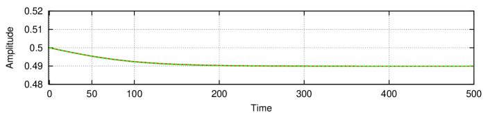
Figure 1: The shape of $\nu_{k}(t)$, $\nu_{k}(0)=0.50$ obtained from the solution of eq. (52) with $a=0.01$: analytic approximation (red); numerical solution (green)

It is easy to see that this solution for all times is very close to the initial value of $\nu_{k}=0.5$. The latter is confirmed by the Runge-Kutta of fourth order numerical solution of the above initial value problem. The relative difference between both predictions does not exceed $10^{-4}\%$ (Fig. 1).

It is not difficult to get other approximate solutions to eq. (51) compatible with the adiabatic approximations. Indeed, one can slightly modify the initial condition $z_{0}$, by, e.g. $z_{0}=\nu_{k}^{2}(0)$, or slightly modify the positions of the zeroes of $P(z)$.

4 Numerical results

To test the reliability of the derived PCTC we solve numerically CTC by Runge-Kutta method of fourth order and the nonlinear scalar NLSE by conservative fully implicit finite-difference method [31] and compare the results. An object of investigation are 5-soliton trains in adiabatic approximation. The complete investigation is a hard task besides PCTC is $4N$ ($N=5$) while the GCTC – $6N$ manifold. In all our computations we consider uniformly placed at distance $r_{0}=8$ solitons or soliton envelopes and vary the initial phase differences $\Delta\delta_{k}=\delta_{k+1}-\delta_{k}$, initial velocities $\nu_{k}$, polarization vectors $\vec{n}_{k}$, $k=1,...,5$. So, the initial positions of the soliton centers are chosen to be $\xi_{1,5}=\pm 16$, $\xi_{2,4}=\pm 8$, $\xi_{3}=0$. In Figs. 2 and 3 the dynamics of the chosen soliton configuration as well as the trajectories of the soliton centers and the magnitudes of the soliton amplitudes are plotted. Though for the concrete set of parameters the scale $\varepsilon\simeq 10^{-2}$ and the respective “adiabatic” time is $1/\varepsilon$ our observations show that the comparison between CTC and NLSE is very good for considerably large time. Similar tests to compare GCTC and Manakov system (MS) are conducted. We aim to check and specify the parameter ranges where the adiabaticity of the solutions holds.

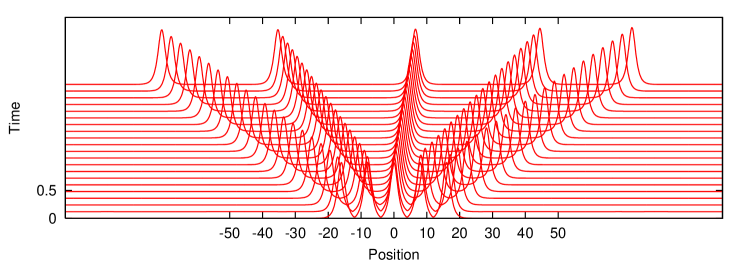
Figure 2: 5-soliton train – Homogeneous scalar NLSE: constant $\Delta\delta=0.8\pi$ with $\delta_{1}=0.8\pi$; $\nu_{1,2,3,4,5}=0.5$

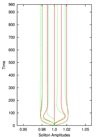
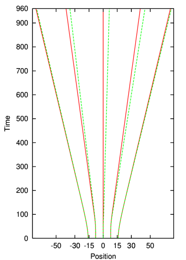
Figure 3: Homogeneous NLSE (green) against CTC (red): constant $\Delta\delta=0.8\pi$ with $\delta_{1}=0.8\pi$; $\nu_{1,2,3,4,5}=0.5$

The PCTC as well as the perturbed NLSE and perturbed MS are not integrable. After the obtained results for 1- and 2-soliton solution [5] the stability for NLSE with gain/loss is possible for small linear and cubic terms with opposite signs. An amplitude balance is attained when $\beta\simeq-1.5\gamma$. Larger values of the relation lead to an infinite energy (blow-up) while the smaller ones – to selfdispersion. If the gain/loss (the pair ($\gamma,\beta)\neq(0,0)$) and $\eta=0$, then for $\nu_{k}=\sqrt{-3\gamma/8\beta}$, $k=1,2,3,4,5$ the reduced polynomial of second degree $P(\nu_{k})\equiv 0$. We established that when the coefficient $\eta\neq 0$ also and the amplitudes $\nu_{k}$ are close to the real zeros of the bisquare polynomial $P(\nu_{k})$ and an appropriate set of the triple ($\gamma$, $\beta$, $\eta$) the perturbation term in PCTC vanishes, i.e. obtain again the original CTC with a Lax presentation and an analytical estimate of the asymptotics. Otherwise it turned out that the adiabaticity holds even a 5-degree nonlinear is present provided $\eta$, $\gamma$, $\beta$ to be small enough and latter two with opposite signs. These properties are illustrated in Figs. 4, 5, 6 where the initial amplitudes are equal,

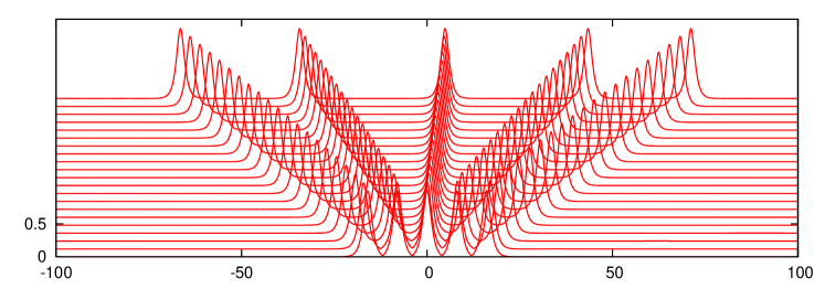
Figure 4: 5-soliton train – Perturbed scalar NLSE: $\gamma=10^{-3}$, $\beta=-1.49\gamma$, constant $\Delta\delta=0.8\pi$ with $\delta_{1}=0.8\pi$; $\nu_{1,2,3,4,5}=0.5$

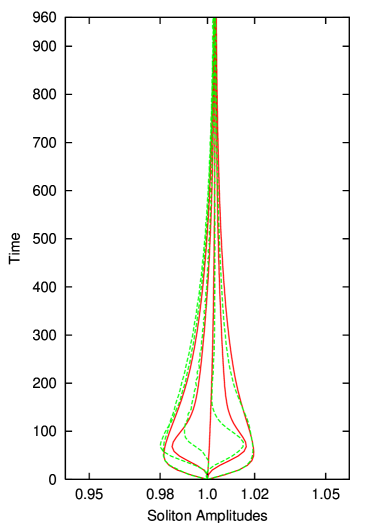
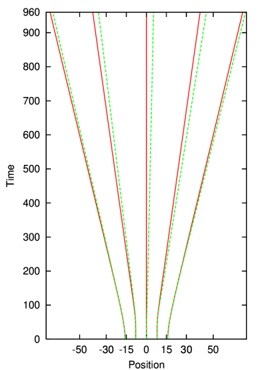
Figure 5: Perturbed scalar NLSE (green) against PCTC (red): $\gamma=10^{-3}$, $\beta=-1.49\gamma$, constant $\Delta\delta=0.8\pi$ with $\delta_{1}=0.8\pi$; $\nu_{1,2,3,4,5}=0.5$

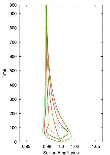
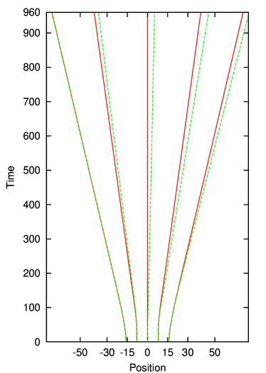
Figure 6: Perturbed scalar NLSE (green) against PCTC (red): $\gamma=10^{-3}$, $\beta=-1.5\gamma$, $\eta=-10^{-4}$, constant $\Delta\delta=0.8\pi$ with $\delta_{1}=0.8\pi$; $\nu_{1,2,3,4,5}=0.5$

$\nu_{k}=0.5$, and $\gamma=10^{-3}$, $\beta=-1.49\gamma$, $\eta=10^{-3}$. Comparing Figs. 5 and 6 one can clearly notices that the plugging on a perturbing nonlinearity of fifth degree strives to deform the trajectories to the left or right depending on the $\eta$ sign. At that time the neither adiabiticity nor the asymptotical behavior of the trajectories are changed. It is seen that the difference between the curves in Fig.  2 and 4 is slightly small. We conclude that the choice of an appropriate set of the coefficients in polynomial $P(\nu_{k})$ including their signs violate the CTC integrability but not the adiabaticity including the asymptotic regime of the solitons.

In contrast to the linear gain/loss and the nonlinear perturbations of higher degree the periodic potential is able to change the asymptotic behavior [13]. Depending on the sign of amplitude $A$ it is possible a transition from a free asymptotic regime (FAR) to a bound state regime (BSR) or a mixed state regime (MSR) and vice versa. In the next 3 graphs are given results for small magnitude of $A$, when a periodic oscillation of the soliton centers appears accompanied by a slight decrease of the phase velocities (Fig. 7), and a change of the asymptotic behavior, when amplitude $A$

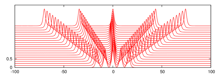
Figure 7: 5-soliton train – Perturbed scalar NLSE: $\gamma=10^{-3}$, $\beta=-1.49\gamma$, $\eta=-10^{-4}$, $A=-10^{-4}$, $\Omega=\pi/4$, constant $\Delta\delta=0.8\pi$ with $\delta_{1}=0.8\pi$; $\nu_{1,2,3,4,5}=0.5$

reaches a critical value (in the concrete case $A_{\rm crit}=-0.0075$). At that value the comparison with scalar NLSE is excellent up to time $t\simeq 600$ (see Figs. 8, 9). Yet, the further growth of $A$ still keeps the adiabaticity at least to time $t\sim 1000$. A positive amplitude $A$ and initial soliton amplitudes $\nu_{k}\simeq 0.5$, $k=1,2,3,4,5$ result an opposite effect, i.e. from BSR or MAR to FAR.

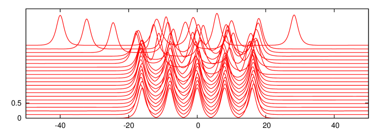
Figure 8: 5-soliton train – Perturbed scalar NLSE: $\gamma=10^{-3}$, $\beta=-1.5\gamma$, $\eta=-10^{-4}$, $A=-0.0075$, $\Omega=\pi/4$, constant $\Delta\delta=0.8\pi$ with $\delta_{1}=0.8\pi$; $\nu_{1,2,3,4,5}=0.5$

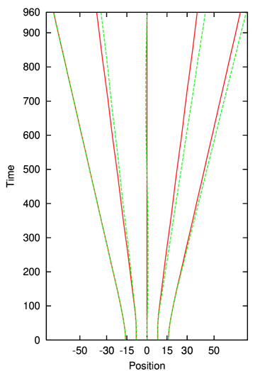
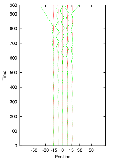
Figure 9: Perturbed scalar NLSE (green) against PCTC (red): $\gamma=10^{-3}$, $\beta=-1.49\gamma$, $\eta=-10^{-4}$, $A=-10^{-4}$ (left), $A=0.0075$ (right), $\Omega=\pi/4$, constant $\Delta\delta=0.8\pi$ with $\delta_{1}=0.8\pi$; $\nu_{1,2,3,4,5}=0.5$

Further we consider two examples of PCTC for two-component MS with gain/loss and external periodic potential. One more equation is needed in this case – for the polarization vectors. As we commented above it can be neglected in adiabatic approximation and the polarization vectors (determined by angles $\theta_{k}$ and $\beta_{k}=0$, $k=1,2,3,4,5$) to be considered as constant in the time. The latter means that PCTC of the perturbed MS is the same like those in the scalar case. In Figs. 10, 11, and 12 is present the effect of the periodic potential for small linear gain ($\gamma=10^{-4}$) and two magnitudes of the periodic amplitude $A$. Similar to the scalar case for large enough values of $A$ occurs a change of the asymptotics of soliton envelopes from FAR to BSR. The adiabatics keeps, the soliton envelopes, too. There is no qualitative difference in the individual soliton amplitudes and their dynamic behavior is similar to the scalar case.

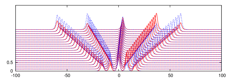
Figure 10: Five freely propagating solitons – Perturbed two-component MS with linear gain $\gamma=10^{-4}$ and periodic external potential: $A=-10^{-4}$, $\Omega=\pi/4$, constant $\Delta\delta=0.8\pi$ with $\delta_{1}=0.8\pi$; $\nu_{1,2,3,4,5}=0.5$

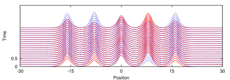
Figure 11: Five solitons – bound state regime due to the periodic potential. Perturbed two-component MS with linear gain $\gamma=10^{-4}$ and periodic external potential: $A=-0.075$, $\Omega=\pi/4$, constant $\Delta\delta=0.8\pi$ with $\delta_{1}=0.8\pi$; $\nu_{1,2,3,4,5}=0.5$

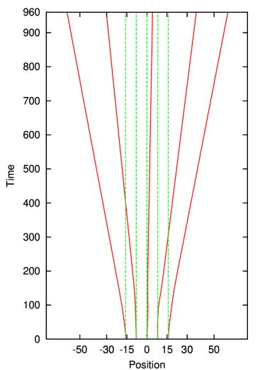
Figure 12: 5-soliton train – Perturbed by a periodic potential two-component MS with linear gain $\gamma=10^{-4}$, $A=-10^{-4}$ (red) and $A=-0.075$ (green), $\Omega=\pi/4$, constant $\Delta\delta=0.8\pi$ with $\delta_{1}=0.8\pi$; $\nu_{1,2,3,4,5}=0.5$; polarization angles $\theta_{1}=\frac{8\pi}{24}$, $\theta_{2}=\frac{15\pi}{24}$, $\theta_{3}=\frac{18\pi}{24}$, $\theta_{4}=\frac{27\pi}{24}$, $\theta_{5}=\frac{8\pi}{24}$

In the next graph (Fig. 13) is considered a 5-soliton configuration again with gain/loss perturbation ($\beta=-1.49\gamma$) but with different initial soliton amplitudes and phase shifts. The corresponding asymptotic regime is MAR. Superposing a periodic potential one observes a change of the asymptotic behavior keeping the adiabaticity. The transition depends on the magnitude of periodic amplitude $A$ (Figs. 14 and 15). The corresponding influence over the trajectories of the soliton envelopes is illustrated in Fig. 16. All the results are verified and compared with the finite-difference implementation of the perturbed MS.

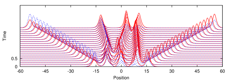
Figure 13: Mixed asymptotic regime of 5-soliton envelopes – Perturbed two-component MS with linear gain $\gamma=10^{-3}$ and cubic loss $\beta=-1.49\gamma$, $\delta_{1,2,4,5}=0$, $\delta_{3}=\pi$; $\nu_{3}=0.5$, $\nu_{4,2}=\nu_{3}\pm 0.01$, $\nu_{5,1}=\nu_{3}\pm 0.02$

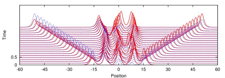
Figure 14: Mixed asymptotic regime of 5-soliton envelopes. Perturbed two-component MS with linear gain $\gamma=10^{-4}$, cubic loss $\beta=-1.49\gamma$ and subcritical periodic external potential: $A=-0.0001$, $\Omega=\pi/4$, $\delta_{1,2,4,5}=0$, $\delta_{3}=\pi$; $\nu_{3}=0.5$, $\nu_{4,2}=\nu_{3}\pm 0.01$, $\nu_{5,1}=\nu_{3}\pm 0.02$; polarization vectors $\theta_{1}=\frac{\pi}{3}$, $\theta_{k+1}=\theta_{k}-\frac{\pi}{8}$, $k=1,2,3,4$.

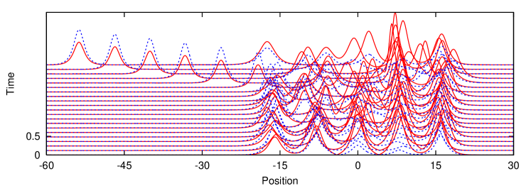
Figure 15: Bound state asymptotic regime of 5-soliton envelopes. Perturbed two-component MS with linear gain $\gamma=10^{-4}$, cubic loss $\beta=-1.49\gamma$ and critical periodic external potential: $A=-0.0075$, $\Omega=\pi/4$, $\delta_{1,2,4,5}=0$, $\delta_{3}=\pi$; $\nu_{3}=0.5$, $\nu_{4,2}=\nu_{3}\pm 0.01$, $\nu_{5,1}=\nu_{3}\pm 0.02$; polarization angles $\theta_{1}=\frac{\pi}{3}$, $\theta_{i+1}=\theta_{i}-\frac{\pi}{8}$, $i=1,2,3,4$.

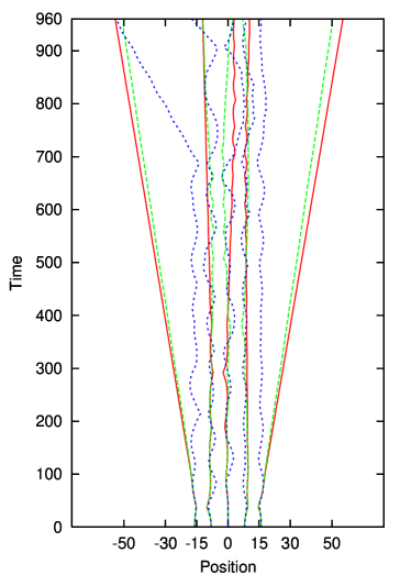
Figure 16: 5-soliton train – Perturbed by a periodic potential two-component MS with linear gain $\gamma=10^{-4}$, cubic loss $\beta=-1.49\gamma$, $A=0$ (red), $A=-10^{-4}$ (green) and $A=-0.0075$ (blue), $\Omega=\pi/4$, $\delta_{1,2,4,5}=0$, $\delta_{3}=\pi$; $\nu_{3}=0.5$, $\nu_{4,2}=\nu_{3}\pm 0.01$, $\nu_{5,1}=\nu_{3}\pm 0.02$; polarization vectors $\theta_{1}=\frac{\pi}{3}$, $\theta_{i+1}=\theta_{i}-\frac{\pi}{8}$, $i=1,2,3,4$.

Concluding Remarks and Future Activity

A wide range of numerical experiments is conducted. All of them aim to report on the influence of linear and nonlinear adiabatic perturbations (gain/loss + nonlinearity of 5-th degree) in the scalar nonlinear Schrödinger equation and the more generalManakov system. Besides above perturbations we consider their superposition with an external periodic potential. We demonstrate that the gain/loss terms strongly affect the adiabatic approximation and for generic choices of $\gamma$, $\beta$ and $\eta$ are not compatible with it. However we found special constraints such as: (i) $\eta=0$, and $\beta\simeq-1.5\gamma$; (ii) eq. (50); after which the gain/loss terms become compatible with adiabaticity. Then we can combine these gain/loss terms with a periodic potential and show how one can switch over 5 asymptotically free solitons into a bound state, or into a 3-soliton bound state and two out-going free solitons.

Other instruments to control the soliton interactions and the asymptotic behavior of the soliton trains are based on the proper choice of the sets of soliton parameters and on the fact that the CTC is integrable, i.e. according [23] it possesses Lax representation $[L,M]=0$ (see also [11, 14, 10]). Given the initial soliton parameters we can evaluate the eigenvalues $\zeta_{k}=\zeta_{0k}+i\zeta_{1k}$ of $L$. Since the real parts $\zeta_{0k}$ determine the asymptotic velocity of the $k$-th soliton, one can determine the asymptotic regime of the soliton train. It will be a FAR of the solitons if all $\zeta_{0k}$ are different; it will be a BSR if all $\zeta_{0k}$ are equal; it will be a MAR otherwise.

Quite similar facts hold true also for the Manakov system [9, 12, 13]. Of course, often the GCTC is not integrable, so formally it does not posses Lax representation. Nevertheless we may start from a soliton configuration that ensures, say a bound state regime and then check whether the perturbation will alter it or not.

Finally, we demonstrate that a large number of different types of perturbations can be effectively treated as compatible with the adiabatic conditions. This, we believe, would enable large number of them to be effectively investigated.

Appendix A Typical integrals

Here we list the typical integrals that appear in deriving the PCTC. First we list the integrals

$$\begin{split}\int_{-\infty}^{\infty}\frac{dz}{\cosh^{2}(z)}=2,\qquad\int_{-\infty}^{\infty}\frac{dz}{\cosh^{4}(z)}=\frac{4}{3},\qquad\int_{-\infty}^{\infty}\frac{dz}{\cosh^{6}(z)}=\frac{16}{15}.\end{split}$$ (53)

needed to derive $R_{k}[u]^{(0)}$. It is possible to derive analytical expressions for all integrals $R_{k}[u]^{(1)}$, but these turn out to be very involved. Below we are keeping only terms of the order of $\varepsilon_{0}$:

$$\int_{-\infty}^{\infty}\frac{dz_{k}\;}{\cosh^{3}(z_{k})\cosh(z_{k\pm 1})} =4e^{-{|\Delta_{k,k\pm 1}|}}+\mathcal{O}(\varepsilon_{0}^{3/2}),$$ (54)

$$\int_{-\infty}^{\infty}\frac{dz_{k}\;}{\cosh^{5}(z_{k})\cosh(z_{k\pm 1})} =\frac{8}{3}e^{-{|\Delta_{k,k\pm 1}|}}+\mathcal{O}(\varepsilon_{0}^{3/2}),$$

$$\int_{-\infty}^{\infty}\frac{dz_{k}\;\tanh(z_{k})}{\cosh^{3}(z_{k})\cosh(z_{k\pm 1})} =\mp\frac{4}{3}e^{-{|\Delta_{k,k\pm 1}|}}+\mathcal{O}(\varepsilon_{0}^{3/2}),$$

$$\int_{-\infty}^{\infty}\frac{dz_{k}\;\tanh(z_{k})}{\cosh^{5}(z_{k})\cosh(z_{k\pm 1})} =\mp\frac{8}{15}e^{-{|\Delta_{k,k\pm 1}|}}+\mathcal{O}(\varepsilon_{0}^{3/2}),$$

and

$$\int_{-\infty}^{\infty}\frac{dz_{k}\;z_{k}}{\cosh^{3}(z_{k})\cosh(z_{k\pm 1})} =\mp 2e^{-{|\Delta_{k,k\pm 1}|}}+\mathcal{O}(\varepsilon_{0}^{3/2}),$$ (55)

$$\int_{-\infty}^{\infty}\frac{dz_{k}\;z_{k}}{\cosh^{5}(z_{k})\cosh(z_{k\pm 1})} =\mp\frac{2}{3}e^{-{|\Delta_{k,k\pm 1}|}}+\mathcal{O}(\varepsilon_{0}^{3/2}),$$

$$\int_{-\infty}^{\infty}\frac{dz_{k}\;(1-z_{k}\tanh(z_{k}))}{\cosh^{3}(z_{k})\cosh(z_{k\pm 1})} =2e^{-{|\Delta_{k,k\pm 1}|}}+\mathcal{O}(\varepsilon_{0}^{3/2}),$$

$$\int_{-\infty}^{\infty}\frac{dz_{k}\;(1-z_{k}\tanh(z_{k}))}{\cosh^{5}(z_{k})\cosh(z_{k\pm 1})} =2e^{-{|\Delta_{k,k\pm 1}|}}+\mathcal{O}(\varepsilon_{0}^{3/2}).$$

References

References

• [1] F.Kh. Abdullaev, S.A. Darmanyan, and P.K. Khabibullaev, Optical Solitons (Springer-Verlag, Heidelberg, 1993).
• [2] M.J. Ablowitz, B. Prinari and A.D. Trubatch, Discrete and Continuous Nonlinear Schrödinger Systems (Cambridge University Press, Cambridge, 2004).
• [3] M.J. Ablowitz and H. Segur, Solitons and the Inverse Scattering Transform (SIAM, Philadelphia, 1981).
• [4] V. V. Afanasjev, Soliton singularity in the system with nonlinear gain. Optics Letters 20 (1995) 704–706.
• [5] R. Carretero-González, V. S. Gerdjikov, and M. D. Todorov. $N$-soliton interactions: Effects of linear and nonlinear gain/loss, in AIP CP1895, American Institute of Physics, Melville, NY, paper 040001, 2017; http://doi.org/10.1063/1.5007368.
• [6] R.K. Dodd, J.C. Eilbeck, J.D. Gibbon, and H.C. Morris, Solitons and Nonlinear Wave Equations (Academic, New York, 1983).
• [7] V. S. Gerdjikov, Complex Toda chain – an integrable universal model for adiabatic $N$-soliton interactions, in M. Ablowitz, M. Boiti, F. Pempinelli, B. Prinari (eds), Nonlinear Physics: Theory and Experiment. II, World Scientific, 2003, pp. 64–70.
• [8] V. S. Gerdjikov, Basic aspects of soliton theory, in “Geometry, Integrability and Quantization”, pp. 78–125; Softex, Sofia 2005, arXiv:nlin.SI/0604004.
• [9] V.S. Gerdjikov, E.V. Doktorov, and N. P. Matsuka, $N$-soliton train and Generalized Complex Toda Chain for Manakov system, Theor. Math. Phys. 151 (2007) 762–773.
• [10] V. S. Gerdjikov, E. G. Evstatiev, D. J. Kaup, G. L. Diankov, and I. M. Uzunov, Stability and quasi-equidistant propagation of NLS soliton trains, Phys. Lett. A 241 (1998) 323–328.
• [11] V. S. Gerdjikov, D. J. Kaup, I. M. Uzunov, and E. G. Evstatiev, Asymptotic behavior of $N$-soliton trains of the nonlinear Schrödinger equation, Phys. Rev. Lett. 77 (1996) 3943–3946.
• [12] V. S. Gerdjikov, N.A. Kostov, E.V. Doktorov, and N.P. Matsuka, Generalized perturbed Complex Toda chain for Manakov system and exact solutions of the Bose-Einstein mixtures, Math. Comput. Simulat. 80 (2009) 112–119.
• [13] V. S. Gerdjikov and M. D. Todorov, $N$-soliton interactions for the Manakov system: effects of external potentials, chapter in P. Kevrekidis et al. (eds.), Localized Excitations in Nonlinear Complex Systems, Nonlinear Systems and Complexity 7, Springer International Publishing Switzerland, 2014, pp.147–169, doi:10.1007/978-3-319-02057-0_7.
• [14] V. S. Gerdjikov, I. M. Uzunov, E. G. Evstatiev, and G. L. Diankov, Nonlinear Schrödinger equation and $N$-soliton interactions: Generalized Karpman-Soloviev approach and the Complex Toda Chain, Phys. Rev. E 55 (1997) 6039–6060.
• [15] V. S. Gerdjikov, M. D. Todorov, and A. V. Kyuldjiev, Polarization effects in modeling soliton interactions of the Manakov model, in AIP CP1684, American Institute of Physics, Melville, NY, 2015, paper 080006, 2015. http://dx.doi.org/10.1063/1.4934317; Asymptotic behavior of Manakov solitons: Effects of potential wells and humps, Math. Comput. Simulat. 121 (2016) 166–178. http://doi.org/10.1016/j.matcom.2015.10.004.
• [16] V. S. Gerdjikov, M. D. Todorov, and A. V. Kyuldjiev, Adiabatic interactions of Manakov soliton – effects of cross-modulation, Special issue “Mathematical modeling and physical dynamics of solitary waves: From continuum mechanics to field theory,” I.C. Christov, M.D. Todorov, S. Yoshida (eds), Wave Motion 71 (2017) 71–81. http://dx.doi.org/10.1016/j.wavemoti.2016.08.004.
• [17] A. Hasegawa and Y. Kodama, Solitons in Optical Communications (Clarendon Press, Oxford, 1995).
• [18] V. I. Karpman and V. V. Solov’ev, A perturbational approach to the two-soliton systems, Physica D 3D 487–502, 1981.
• [19] P. G. Kevrekidis, D. J. Frantzeskakis, and R. Carretero-González (eds), Emergent Nonlinear Phenomena in Bose-Einstein Condensates. Theory and Experiment (Springer-Verlag, Berlin, 2008); R. Carretero-González, D. J. Frantzeskakis, and P. G. Kevrekidis, Nonlinear waves in Bose Einstein condensates: physical relevance and mathematical techniques, Nonlinearity 21 (2008) R139.
• [20] P. G. Kevrekidis, D. J. Frantzeskakis, and R. Carretero-González, The Defocusing Nonlinear Schrödinger Equation, SIAM (Philadelphia, 2015).
• [21] Yu.S. Kivshar and G.P. Agrawal, Optical Solitons: From Fibers to Photonic Crystals (Academic Press, 2003).
• [22] S. V. Manakov, On the theory of two-dimensional stationary self-focusing of electromagnetic waves, Zh. Eksp. Teor. Fiz. 65 (1973) 505-516 (in Russian); English translation: Sov. Phys. JETP 38(2) (1974) 248–253. 33.
• [23] J. Moser, Dynamical Systems, Theory and Applications, Lecture Notes in Physics 38, Springer Verlag (1975); pp. 467–497; Three integrable Hamiltonian systems connected to isospectral deformations, Adv. Math. 16 (1975) 197–220.
• [24] A.C. Newell, Solitons in Mathematics and Physics (SIAM, Philadelphia, 1985).
• [25] C. J. Pethick and H. Smith, Bose-Einstein Condensation in Dilute Gases (Cambridge University Press, Cambridge, 2002).
• [26] L. P. Pitaevskii and S. Stringari, Bose-Einstein Condensation, Oxford University Press (Oxford, 2003).
• [27] J. Rossi, R. Carretero-González, and P.G. Kevrekidis, Non-conservative variational approximation for nonlinear Schröger equations. In preparation.
• [28] J. Rossi, R. Carretero-González, P.G. Kevrekidis, and M. Haragus, On the spontaneous time-reversal symmetry breaking in synchronously-pumped passive Kerr resonators, J. Phys. A 49 (2016) 455201. doi:10.1088/1751-8113/49/45/455201.
• [29] A. Scott, Nonlinear Science. Emergence and Dynamics of Coherent Structures (2nd edn) (Osford University Press, Oxford, 2003).
• [30] C. Sulem and P.L. Sulem, The Nonlinear Schrödinger Equation (Springer-Verlag, New York, 1999).
• [31] M.D. Todorov and C.I. Christov, Conservative numerical scheme in complex arithmetic for coupled nonlinear Schrodinger equations, Discrete and Continuous Dynamical Systems, Suppl. 2007 (2007), pp. 982-992.
• [32] M. D. Todorov, V. S. Gerdjikov, and A. V. Kyuldjiev, Modeling interactions of soliton trains. Effects of external potentials, in AIP CP1629, American Institute of Physics, Melville, NY, 2014, pp. 186–200. doi:10.1063/1.4902273.
• [33] M. D. Todorov, V. S. Gerdjikov, and A. V. Kyuldjiev, Multi-soliton interactions for the Manakov system under composite external potentials, Proceedings of the Estonian Academy of Sciences, Phys.-Math. series. 64(3) (2015) 368–378. doi:10.3176/proc.2015.3S.07.
• [34] I.M. Uzunov, V.D. Stoev and T.I. Tzoleva, N-soliton interaction in trains of unequal soliton pulses in optical fibers, Optics Letters 20 (1992), 1417–1419.
• [35] V.E. Zakharov, S.V. Manakov, S.P. Nonikov, and L.P. Pitaevskii, Theory of Solitons (Consultants Bureau, NY, 1984).
• [36] V. E. Zakharov and A. B. Shabat, Exact theory of two-dimensional self-focusing and one-dimensional self-modulation of waves in nonlinear media, ZhETF 61(1) (1972) 118–134 (in Russian); English translation: Soviet Physics-JETP 34(1) (1972) 62–69.