Self-Consistent Description of Local Density Dynamics in Simple Liquids.
The Case of Molten Lithium

Abstract

The dynamic structure factor is the quantity, which can be measured by means of Brillouin light-scattering as well as by means of inelastic scattering of neutrons and X-rays. The spectral (or frequency) moments of the dynamic structure factor define directly the sum rules of the scattering law. The theoretical scheme formulated in this study allows one to describe the dynamics of local density fluctuations in simple liquids and to obtain the expression of the dynamic structure factor in terms of the spectral moments. The theory satisfies all the sum rules, and the obtained expression for the dynamic structure factor yields correct extrapolations into the hydrodynamic limit as well as into the free-particle dynamics limit. We discuss correspondence of this theory with the generalized hydrodynamics and with the viscoelastic models, which are commonly used to analyze the data of inelastic neutron and X-ray scattering in liquids. In particular, we reveal that the postulated condition of the viscoelastic model for the memory function can be directly obtained within the presented theory. The dynamic structure factor of liquid lithium is computed on the basis of the presented theory, and various features of the scattering spectra are evaluated. It is found that the theoretical results are in agreement with inelastic X-ray scattering data.

Keywords: microscopic dynamics, liquids, liquid metals, density fluctuations, scattering spectra, spectral moments, molecular dynamics simulations

1 Introduction

The collective dynamics in a liquid occurs over a wide range of the spatial scales varied from the scales comparable with the particle sizes (of the order of few Angstroms) up to the macroscopical scales typical for hydrodynamics. The features of this dynamics determine directly the lineshape of the dynamic structure factor $S(k,\omega)$. The long-wavelength limit ($k\to 0$) corresponds to ordinary hydrodynamics, and the spectrum of the dynamic structure factor $S(k,\omega)$ at extremely small values of the wavenumber $k$ is characterized by the line shape known as the Rayleigh-Mandelshtam-Brillouin triplet. This spectrum consists of one central (Rayleigh) peak located at $\omega=0$ and two side (Brillouin) peaks located at frequencies $\pm\omega_{c}$, where $\omega_{c}=c_{s}k$ and $c_{s}$ is the adiabatic sound velocity. Hence, the lineshape of $S(k,\omega)$ represents a result of the sum of three Lorentzians (in respect to the frequency $\omega$) [1]:

$$S(k,\omega) = \frac{S(k)}{2\pi}\left\{\left(\frac{\gamma-1}{\gamma}\right)\frac{2D_{T}k^{2}}{\omega^{2}+(D_{T}k^{2})^{2}}\right.$$

$$\left.+\frac{1}{\gamma}\sum_{l=1}^{2}\frac{\Gamma k^{2}}{[\omega+(-1)^{l}c_{s}k]^{2}+(\Gamma k^{2})^{2}}\right\},$$

with the following parameters – the thermal diffusivity $D_{T}$, the sound attenuation coefficient $\Gamma=(1/2)[(\gamma-1)D_{T}+\eta_{L}]$, the ratio of the specific heat at constant pressure to the specific heat at constant volume $\gamma=c_{p}/c_{V}$, the longitudinal viscosity $\eta_{L}$, and the static structure factor $S(k)$. Note that Eq. (1) reproduces the next peculiarities of the density fluctuations dynamics observed in the Brillouin light-scattering experiments: (i) the three peaks corresponding to these Lorentzians are well defined and separated by two gaps of the same width; the Rayleigh component $I_{R}$ and the Brillouin component $I_{B}$ are defined as follows

$$I_{R} = \frac{S(k)}{\pi}\left(\frac{\gamma-1}{\gamma}\right)\int_{-\infty}^{\infty}\frac{D_{T}k^{2}}{\omega^{2}+(D_{T}k^{2})^{2}}d\omega$$

$$= S(k)\left(\frac{\gamma-1}{\gamma}\right)$$

and

$$I_{B}=\frac{S(k)}{2\pi}\frac{1}{\gamma}\int_{-\infty}^{\infty}\frac{\Gamma k^{2}}{[\omega\pm(c_{s}k)]^{2}+(\Gamma k^{2})^{2}}d\omega=\frac{S(k)}{2}\frac{1}{\gamma}.$$

The correspondence between the components is defined by the Landau-Placzek ratio [2]

$$\frac{I_{R}}{2I_{B}}=\gamma-1;$$

(ii) these peaks are broaden with increase of the wavenumber in accordance with $k^{2}$-dependence; and (iii) shift of two symmetric peaks to higher frequencies with increase of the wavenumber $k$ defines the linear low-$k$ asymptotic of the longitudinal sound dispersion, $\lim_{k\to 0}\omega_{c}(k)=c_{s}k$.

The Brillouin light-scattering in liquids probes the macroscopical longitudinal density fluctuations. Then, Inelastic Neutron Scattering (INS) and Inelastic X-ray Scattering (IXS) experiments allow one to extract an information about the local density fluctuations corresponding to the microscopical spatial scales with the wavelengths raised by collective dynamics of few amount of particles up to the wavelengths corresponding to free-particle dynamics regime [3]. Let $k_{m}$ be the wavenumber corresponding to the first (principal) maximum of the static structure factor $S(k)$. For the case of monatomic liquids, the maximum of the static structure factor, $S(k_{m})$, is the largest one, and the quantity $r_{m}=2\pi/k_{m}$ will provide an approximate estimate of an equilibrium distance between the centers of two neighboring atoms. The wavenumbers available via INS and IXS experiments cover a wide range, which includes $k\in[0.1;\;5]\;k_{m}$. These experiments have revealed that the three-peak lineshape of $S(k,\omega)$-spectra similar to the Rayleigh-Mandelshtam-Brillouin triplet appears also at finite wavenumbers till the boundary of the first Brillouin pseudo-zone with $k=k_{m}/2$, albeit these peaks are not separated, and the experimental $S(k,\omega)$-spectra are not reproducible by Eq. (1) [4, 5]. With further increase of the wavenumber $k$, the side peaks of the dynamic structure factor spectra start to shift to the lower frequencies and these peaks disappear completely at $k\simeq 0.75\;k_{m}$. At these wavenumbers, the tangent to the dispersion curve $\omega_{c}(k)$ takes a negative slope and the intensity of the central spectral component, $S(k,\omega=0)$, grows. Such changes of the scattering spectra occur until the wave number approaches the value $k_{m}$, at which the spectrum of the dynamic structure factor will be represented by the central Rayleigh component. Thus, at the wavenumbers comparable with $k_{m}$, the $S(k,\omega)$ spectrum covers a narrow frequency range. This is known as the de Gennes narrowing effect [6, 7]. Further, the wavenumbers $k\geq k_{m}$ correspond to the transition range in the regime of free-particle dynamics. Thus, at very large wavenumbers $k>k_{m}$, the characteristic wavelenths are shorter than an interparticle distance. Here, the dynamic structure factor $S(k,\omega)$ is reproduced by the Gaussian function

$$S(k,\omega)=\sqrt{\frac{1}{2\pi}}\frac{1}{v_{T}k}\exp\left(-\frac{\omega^{2}}{2(v_{T}k)^{2}}\right),$$ (2)

where $v_{T}$ is particle velocity.

INS and IXS spectra for the extended wavenumber range $k\in[0.1;\;1]k_{m}$ provide a useful information to develop and to test the theoretical models of local density fluctuations dynamics in liquids. The theoretical analysis of these experimental data is usually performed within the time correlation functions (TCF’s) formalism [8] and on the basis of ideas of the generalized hydrodynamics [9]. At the present time, there are various theoretical models of the dynamic structure factor $S(k,\omega)$ of simple liquids (for details see reviews [10, 11, 4]). And, as it turned out, it is not difficult to develop a theoretical scheme with a certain amount of adjustable parameters. Nevertheless, the main difficulty here is to propose a theoretical methodology that will ensure the correct transition from hydrodynamic description with a set of macroscopic parameters to description of microscopic dynamics with appropriate characteristics such as the interparticle interaction, the particle velocities and the particle distribution functions. Moreover, a suggested theoretical model has to provide the correct time dependence of the TCF’s and has to satisfy the so called sum-rules of a spectral functions [12].

In this work, we will demonstrate that description of density fluctuations dynamics as well as analysis of INS and IXS data of simple liquids can be done self-consistently in terms of the low-order frequency moments (or the low-order frequency parameters) of the dynamic structure factor. In fact, this theoretical scheme formalizes the idea of a self-consistent description of the density fluctuations in the same manner as this is realizing by the mode-coupling theory, where the statistical treatment of the dynamics of a system with an infinite number of degrees of freedom is reduced to closed integro-differential equations [13]. As follows from the theoretical definitions, the frequency moments are related to the microscopic characteristics: the particle interaction energy, the particle velocity, the local structure parameters. This theoretical scheme allows one to obtain the model for the dynamic structure factor of simple liquids.

Liquid alkali metals are suitable candidates to test the proposed theories of the microscopical collective dynamics in a liquid [12, 14, 8, 9]. The potential energy of these systems can be regarded as a quantity determined mainly by the ion-ion interactions, whilst the electron screening effects are taken into account effectively. The interactions between the particles (ions) in alkali metals are reproduced by a potential $u(\mathbf{r})$, which is the simplest in comparison with the potentials for other metals. Therefore, various characteristics of the density fluctuation dynamics in liquid alkali metals can be evaluated on the basis of the proposed microscopic theories, where the potential is the main input parameter. Note that experimental data for liquid alkali metals [15], including recent results of Inelastic Neutron and X-ray Scattering [10, 11, 3, 16, 17, 18, 19, 20, 21], provides a reliable basis for theoretical and numerical simulation studies [22, 23, 24, 25, 26, 27, 28, 29, 30, 31, 32, 33].

Liquid lithium has the simple electronic structure $1s^{2}2s$ and is characterized by a large ratio of valence electrons to core electrons. This ratio is larger even than for other liquid alkali metals. As a result, some physical properties of lithium determined by the microscopic dynamics turn out to be specific. In particular, liquid lithium has the largest sound velocity and the smallest heat capacity in comparison with other alkalis. Namely, the sound velocity is $c_{s}=4554$ m/s and the molar heat capacity at constant pressure is $c_{p}=30.33$ J/(mol$\cdot$K), whereas the ratio of specific heats $\gamma=c_{p}/c_{V}=1.065$ at the melting temperature $T_{m}=453$ K and ambient pressure [15]. The local and non-local pseudopotentials as well as the more sophisticated EAM and modified EAM (MEAM) potentials have been proposed for the case of liquid lithium. To examine these potentials, the structure and dynamical properties had been evaluated in works of Kresse [34], Canales et al. [24], Torcini et al. [22], Gonzalez et al. [35], Anta and Madden [31], Salmon et al. [36] and others. It was found that the spectra of the dynamic structure factor obtained by means of molecular dynamics with a pair pseudopotential have better agreement with IXS data than simulation results with the EAM potentials [35, 37]. In addition, many various theoretical models of the dynamic structure factor were tested with the high quality IXS data for liquid lithium [22, 38, 39]. Therefore, we examine our theoretical scheme for the case of liquid lithium.

The paper is organized as follows. Theoretical description is given in Section 2. Namely, the basic points and definitions of the time correlation functions formalism are presented in Subsection 2.1. The self-consistent theory of the density fluctuations dynamics in simple liquids developed in the framework of this formalism is presented in Subsection 2.2. In this Subsection, we present the original theoretical results related with the detailed derivation of the expressions for the dynamic structure factor, dispersion relation for the longitudinal collective excitations and other spectral characteristics. Comparison with other theoretical schemes is given in Section 3. We discuss the correspondence of our theoretical scheme with the known simple and extended viscoelastic models (Subsection 3.1), with the ordinary and generalized hydrodynamic theories (Subsections 3.2 and 3.3) and with the model for the free-particle dynamics (Subsection 3.4). In section 4, the theoretical model is applied to compute the dynamic structure factor of liquid lithium and the theoretical results are compared with experimental IXS data for this liquid metal. The concluding remarks are given in Section 5.

2 Theoretical description

2.1 Fundamental notions

According to statistical mechanics, if one treats an equilibrium liquid as a many-particle system, then it is convenient to apply the mathematical formalism of the correlation functions, distribution functions, the moments and cumulants of these functions. In particular, the time correlation functions allow us to describe the relaxation processes occurring in the system at different spatial scales [40]. As a result, the corresponding microscopic theory can be developed. In the given study, we are focused on the collective particle dynamics of a liquid. Therefore, we assume that the particle interaction potential and such the structural parameters as the particle distribution functions and the static structure factor are defined and can be used as input parameters of the theoretical scheme.

Let us consider an isotropic system, which consists on $N$ classical particles of a mass $m$ enclosed in a volume $V$. As an initial dynamical variable we take the Fourier-component of the local density fluctuations

$$\rho_{k}=\frac{1}{\sqrt{N}}\sum_{j=1}^{N}e^{i\mathbf{k}\cdot\mathbf{r}_{j}},\ \ \ k=|\mathbf{k}|,$$ (3)

whose evolution is defined by the corresponding equation of motion

$$\dot{\rho}_{k}(t)=i\hat{\mathcal{L}}\rho_{k}(t).$$ (4)

Here, the dot denotes time differentiation, and $\hat{\mathcal{L}}$ is the Liouville operator, which is Hermitian [40, 41]:

$$\hat{\mathcal{L}}=-i\left\{\frac{1}{m}\sum_{j=1}^{N}(\mathbf{p}_{j}\cdot\mathbf{\nabla}_{j})-\sum_{l>j=1}^{N}\nabla_{j}u(r_{jl})\left(\nabla_{\mathbf{p}_{j}}-\nabla_{\mathbf{p}_{l}}\right)\right\}.$$ (5)

Further, $\mathbf{p}_{j}$ is the momentum of the $j$th particle, $\mathbf{\nabla}_{j}$ and $\nabla_{\mathbf{p}_{j}}$ are the gradients over coordinates and momenta, respectively. The quantity $u(r)$ is the interaction energy between a pair of the particles and, as expected, it can be evaluated from any model potential. By means of the Gram-Schmidt orthogonalization procedure [42] on the basis of the quantity $A_{0}(k)\equiv\rho_{k}$ we generate the infinite set of variables

$$\mathbf{A}(k)=\{A_{0}(k),\;A_{1}(k),\;A_{2}(k),\;\ldots\}\\$$ (6)

related by

$$A_{j+1}(k)=i\hat{\mathcal{L}}A_{j}(k)+\Delta_{j}^{2}(k)A_{j-1}(k),$$ (7)

$$j=0,\;1,\;2,\;\ldots;$$

$$A_{-1}\equiv 0.$$

Here,

$$\Delta_{j+1}^{2}(k)=\frac{\langle|A_{j+1}(k)|^{2}\rangle}{\langle|A_{j}(k)|^{2}\rangle}$$ (8)

is an $j$th-order frequency parameter (at fixed $k$), which has a dimension of square frequency [43]; and the brackets $\langle\ldots\rangle$ denote the ensemble average.

The variables of set (6) are the generalized dynamical variables dependent on the wavenumber $k$ as parameter (see discussion in Ref. [44], pages 100-101). These variables form an orthogonal basis [42, 41]:

$$\langle A^{*}_{i}(k)A_{j}(k)\rangle=\delta_{i,j}\langle|A_{j}(k)|^{2}\rangle,$$ (9)

$$i,j=0,\;1,\;2,\;\ldots.$$

Further, while the first variable $A_{0}(k)$ is defined by Eq. (3), then the second variable is

$$A_{1}(k)=\frac{i}{\sqrt{N}}\sum_{j=1}^{N}(\mathbf{k}\cdot\mathbf{v}_{j})e^{i\mathbf{k}\cdot\mathbf{r}_{j}},$$ (10)

and for the third variable one has

$$A_{2}(k) = \dot{A}_{1}(k)+\Delta_{1}^{2}(k)A_{0}(k)$$

$$= -\frac{1}{\sqrt{N}}\sum_{j=1}^{N}\left(\mathbf{k}\cdot\mathbf{v}_{j}\right)^{2}\textrm{e}^{i\mathbf{k}\cdot\mathbf{r}_{j}}$$

$$+ \frac{i}{\sqrt{mN}}\sum_{l>j=1}^{N}(\mathbf{\nabla}_{j}\cdot\mathbf{k})u(r_{jl})\left\{\textrm{e}^{i\mathbf{k}\cdot\mathbf{r}_{j}}-\textrm{e}^{i\mathbf{k}\cdot\mathbf{r}_{l}}\right\}+\Delta_{1}^{2}(k)A_{0}(k).$$

Let us define the time correlation function (TCF)

$$M_{j}(k,t)=\frac{\langle A_{j}^{*}(0)A_{j}(t)\rangle}{\langle|A_{j}^{*}(0)|^{2}\rangle},$$ (12)

$$j=0,\;1,\;2,\;\ldots,$$

which will be characterized by the properties

$$\left.{M}_{j}(k,t)\right|_{t=0}=1,$$ (13a)

$$\left|M_{j}(k,t)\right|\leq 1,$$ (13b)

and

$$\left.\frac{d^{l}}{dt^{l}}M_{j}(k,t)\right|_{t=0}=0, \textrm{if {l} is odd},$$ (13c)

$$\left.\frac{d^{l}}{dt^{l}}M_{j}(k,t)\right|_{t=0}\neq 0, \textrm{if {l} is even}.$$

These properties are directly derived from condition (9). Then, the TCF

$$M_{0}(k,t)=F(k,t)=\frac{\langle\rho_{k}^{*}(0)\rho_{k}(t)\rangle}{\langle|\rho_{k}(0)|^{2}\rangle}$$ (13n)

represents the density-density correlation function known also as the intermediate scattering function. This TCF is related to the dynamic structure factor [8]

$$S(k,\omega)=\frac{S(k)}{2\pi}\int_{-\infty}^{\infty}\;\exp(i\omega t)F(k,t)\;dt,$$ (13o)

where $S(k)=\langle|\rho_{k}(0)|^{2}\rangle$ is the static structure factor. Taking into account property (13c), one obtains the short-time expansion for the intermediate scattering function:

$$F(k,t)=1-\langle\omega^{(2)}(k)\rangle\frac{t^{2}}{2!}+\langle\omega^{(4)}(k)\rangle\frac{t^{4}}{4!}+\ldots+(-i)^{l}\langle\omega^{(l)}(k)\rangle\frac{t^{l}}{l!}+\ldots,$$

where $\langle\omega^{(l)}\rangle$ is the $l$th-order normalized frequency moment of the dynamic structure factor $S(k,\omega)$ [45, 46, 47, 48, 49]:

$$\langle\omega^{(l)}(k)\rangle=\left.(-i)^{l}\frac{d^{(l)}}{dt^{l}}F(k,t)\right|_{t=0}=\frac{\int_{-\infty}^{\infty}\omega^{l}S(k,\omega)d\omega}{\int_{-\infty}^{\infty}S(k,\omega)d\omega}.$$

The quantity $M_{1}(k,t)$ is the TCF associated with the longitudinal-current autocorrelation function

$$C_{L}(k,t)=\frac{\langle j_{k}^{(L)}(0)j_{k}^{(L)}(t)\rangle}{\langle|j_{k}^{(L)}(0)|^{2}\rangle},$$ (13p)

which is related, in turn, to the intermediate scattering function $F(k,t)$ as follows [14]

$$-\frac{d^{2}}{dt^{2}}F(k,t)=\Delta_{1}^{2}(k)C_{L}(k,t).$$ (13q)

The label $L$ denotes the component parallel to the wavevector $\mathbf{k}$. Relation (13q) is direct consequence of the hydrodynamic continuity equation

$$\frac{\partial}{\partial t}\rho_{k}(t)+ikj_{k}^{(L)}=0,$$ (13r)

which shows that spontaneous fluctuations of a conserved hydrodynamic variable $\rho_{k}(t)$ decay very slowly at long wavelengths (i.e. at extremely small wavenumbers) [8]. Then, taking into account Eq. (13o) one obtains the correspondence between the spectral density of the longitudinal-current fluctuations

$$C_{L}(k,\omega)=\frac{1}{2\pi}\int_{-\infty}^{\infty}\;\exp(i\omega t)C_{L}(k,t)\;dt$$

and the dynamic structure factor $S(k,\omega)$ [50, 51]:

$$S(k)\Delta_{1}^{2}(k)C_{L}(k,\omega)=\omega^{2}S(k,\omega).$$ (13s)

Further, from Eq. (2.1) one can verify that the TCF $M_{2}(k,t)$ is expressed in terms of the TCF’s of energy or stress tensor, of force and of density as well as in terms of the corresponding cross-correlation functions. Then, the TCF $M_{3}(k,t)$ will contain a contribution related to the TCF of energy current [28]. Thus, the quantities $F(k,t)$, $M_{1}(k,t)$, $M_{2}(k,t)$ and $M_{3}(k,t)$ are the TCF’s of the variables arising also in the hydrodynamic conservation laws for the longitudinal collective dynamics. These TCF’s correspond to the concrete relaxation processes [52]. The time scales of the relaxation processes can be conveniently evaluated by

$$\tau_{j}(k)=\frac{1}{\sqrt{\Delta_{j}^{2}(k)}},\;\;j=0,\;1,\;2,\;\ldots.$$ (13t)

The functions $F(k,t)$, $C_{L}(k,t)$, $M_{2}(k,t)$ and $M_{3}(k,t)$ obey the next kinetic integro-differential equations:

$$\ddot{F}(k,t)+\Delta_{1}^{2}(k)F(k,t)+\Delta_{2}^{2}(k)\int_{0}^{t}d\tau M_{2}(k,t-\tau)\dot{F}(k,\tau^{{}^{\prime}})=0,$$ (13ua)

$$\ddot{M_{1}}(k,t)+\Delta_{2}^{2}(k)M_{1}(k,t)+\Delta_{3}^{2}(k)\int_{0}^{t}d\tau M_{3}(k,t-\tau)\dot{M_{1}}(k,\tau^{{}^{\prime}})=0,$$ (13ub)

$$\ddot{M_{2}}(k,t)+\Delta_{3}^{2}(k)M_{2}(k,t)+\Delta_{4}^{2}(k)\int_{0}^{t}d\tau M_{4}(k,t-\tau)\dot{M_{2}}(k,\tau^{{}^{\prime}})=0.$$ (13uc)

Eqs. (13ua), (13ub) and (13uc) can be derived by means of the recurrent relations method [42] or by the projection operators technique [40] from the equations of motion for the variables $A_{0}(k)$, $A_{1}(k)$ and $A_{2}(k)$. Recall that the frequency parameters $\Delta_{1}^{2}(k)$, $\Delta_{2}^{2}(k)$, $\Delta_{3}^{2}(k)$ and $\Delta_{4}^{2}(k)$ can be found directly from definition (8). On the other hand, one obtains from (2.1) that

$$\Delta_{1}^{2}(k)=\langle\omega^{(2)}(k)\rangle,$$ (13uva)

$$\Delta_{2}^{2}(k)=\frac{\langle\omega^{(4)}(k)\rangle}{\langle\omega^{(2)}(k)\rangle}-\langle\omega^{(2)}(k)\rangle,$$ (13uvb)

$$\Delta_{3}^{2}(k)=\frac{\langle\omega^{(6)}(k)\rangle\langle\omega^{(2)}(k)\rangle-(\langle\omega^{(4)}(k)\rangle)^{2}}{\langle\omega^{(4)}(k)\rangle\langle\omega^{(2)}(k)\rangle-(\langle\omega^{(2)}(k)\rangle)^{3}},$$ (13uvc)

$$\Delta_{4}^{2}(k) = \frac{1}{\Delta_{1}^{2}(k)\Delta_{2}^{2}(k)\Delta_{3}^{2}(k)}\Big{\{}\langle\omega^{(8)}(k)\rangle-\Delta_{1}^{2}(k)\Big{[}\Big{(}\Delta_{1}^{2}(k)+\Delta_{2}^{2}(k)\Big{)}^{3}+$$ (13uvd)

$$+2\Delta_{2}^{2}(k)\Delta_{3}^{2}(k)\Big{(}\Delta_{1}^{2}(k)+\Delta_{2}^{2}(k)\Big{)}+\Delta_{2}^{2}(k)\Delta_{3}^{4}(k)\Big{]}\Big{\}},$$

$$\Delta_{5}^{2}(k) = \frac{1}{\Delta_{1}^{2}(k)\Delta_{2}^{2}(k)\Delta_{3}^{2}(k)\Delta_{4}^{2}(k)}\Bigg{\{}\omega^{(10)}(k)-$$

$$-2\omega^{(8)}(k)\Big{[}\Delta_{1}^{2}(k)+\Delta_{2}^{2}(k)+\Delta_{3}^{2}(k)+\Delta_{4}^{2}(k)\Big{]}+$$

$$+\omega^{(6)}(k)\Big{[}\Delta_{1}^{4}(k)+2\Delta_{1}^{2}(k)\Delta_{2}^{2}(k)+\Delta_{2}^{4}(k)+4\Delta_{1}^{2}(k)\Delta_{3}^{2}(k)$$

$$+2\Delta_{2}^{2}(k)\Delta_{3}^{2}(k)+\Delta_{3}^{4}(k)+4\Delta_{1}^{2}(k)\Delta_{4}^{2}(k)\Big{]}\Biggl{\}}+\Delta_{4}^{2}(k).$$

One can see that the frequency parameter of the $j$th order is defined through the frequency moments up to the moment of the $2j$th order. Relations similar to (13uva)–(13uv) can be also written for the frequency parameters of the higher order. Moreother, relations (2.1), (13uva)–(13uv) are the low-order sum rules of the scattering law $S(k,\omega)$.

Taking into account the statistical average in the product of the dynamical variables in relation (8), the frequency moments $\langle\omega^{(l)}(k)\rangle$ can be expressed in terms of the thermal velocity $v_{th}=\sqrt{k_{B}T/m}$ of a particle, the interparticle potential $u(\mathbf{r})$ and the particles distribution functions. Thus, the first frequency parameter $\Delta_{1}^{2}(k)$ is defined as

$$\Delta_{1}^{2}(k)=\frac{k_{B}T}{m}\frac{k^{2}}{S(k)}=\frac{(v_{th}k)^{2}}{S(k)}.$$ (13uvwa)

The second frequency parameter $$\Delta_{2}^{2}(k)$$ can be found from

$$\Delta_{2}^{2}(k) = 3\frac{k_{B}T}{m}k^{2}-\Delta_{1}^{2}(k)+\frac{\rho}{m}\int\nabla_{l}^{2}u(\mathbf{r})[1-\exp(i\mathbf{k}\cdot\mathbf{r})]g(r)\mathrm{d}^{3}\mathbf{r}$$

$$\approx 3\left(\frac{k_{B}T}{m}k^{2}+\omega_{E}^{2}\right)-\Delta_{1}^{2}(k)-\frac{\rho}{m}\int\nabla_{l}^{2}u(\mathbf{r})\exp(i\mathbf{k}\cdot\mathbf{r})g(r)\mathrm{d}^{3}\mathbf{r}.$$

The third frequency parameter is defined as

$$\Delta_{3}^{2}(k) = \frac{1}{\Delta_{2}^{2}(k)}\left\{15\left(\frac{k_{B}T}{m}k^{2}\right)+\mathcal{F}(k)\right\}-\frac{1}{\Delta_{2}^{2}(k)}\left[\Delta_{1}^{2}(k)+\Delta_{2}^{2}(k)\right]^{2}.$$ (13uvwc)

Here, $\rho=N/V$ is the number density, $g(r)$ is the pair distribution function, $\omega_{E}$ is the so-called Einstein frequency, and the term $\mathcal{F}(k)$ denotes the combination integral expressions containing the interparticle potential $u(\mathbf{r})$ and such the structural characteristics as the two- and three-particle distribution functions [32]. Moreover, the $j$th order relaxation parameter $\Delta_{j}^{2}(k)$ with $j\geq 2$ will be defined by the potential $u(\mathbf{r})$ as well as by the distribution functions of two, three, $\ldots$, $(j-2)$, $(j-1)$ and $j$ particles. Thus, the relaxation parameters $\Delta_{j}^{2}(k)$ at $j\geq 2$ are directly dependent on the type of interaction between the particles and on the microscopic structural characteristics.

Eq. (13ua) is also known as the generalized Langevin equation. By the Laplace transformation

$$LT\{f\}(s)=\tilde{f}(s)=\int_{0}^{\infty}e^{-st}f(t)\;dt,\hskip 28.45274pts=i\omega,$$

of Eq. (13ua) and solving it in terms of Eq. (13o), one obtains expression for the classical dynamic structure factor:

$$S(k,\omega)=\frac{S(k)}{\pi}\frac{\Delta_{1}^{2}(k)\Delta_{2}^{2}(k)M^{\prime}_{2}(k,\omega)}{[\omega^{2}-\Delta_{1}^{2}(k)+\omega\Delta_{2}^{2}(k)M^{\prime\prime}_{2}(k,\omega)]^{2}+[\omega\Delta_{2}^{2}(k)M^{\prime}_{2}(k,\omega)]^{2}},$$ (13uvwx)

where $\widetilde{M}^{\prime}_{2}(k,\omega)$ and $\widetilde{M}^{\prime\prime}_{2}(k,\omega)$ are the real and imaginary parts of $\widetilde{M}_{2}(k,s=i\omega)$, respectively. Eq. (13uvwx) is usually applied to explain the features of the experimental dynamic structure factor [4]. This implies in fact a fitting of the experimental $S(k,\omega)$ by Eq. (13uvwx) with a suggested theoretical model for the TCF $M_{2}(k,t)$ [8]. In particular, if the TCF decays instantaneously, $M_{2}(k,t)=\tau_{2}(k)\delta(t)$, then Eq. (13uvwx) reduces to the equation for the damped harmonic oscillator (DHO) model:

$$S(k,\omega)=\frac{S(k)}{\pi}\frac{\Delta_{1}^{2}(k)\Delta_{2}^{2}(k)\tau_{2}(k)}{[\omega^{2}-\Delta_{1}^{2}(k)]^{2}+[\omega\Delta_{2}^{2}(k)\tau_{2}(k)]^{2}},$$ (13uvwy)

where $\tau_{2}(k)$ is the damping parameter. On the other hand, the TCF with an exponential decay

$$M_{2}(k,t)=e^{-t/\tau_{2}(k)}$$ (13uvwz)

yields the simple viscoelastic model for the dynamic structure factor $S(k,\omega)$ [5].

2.2 Self-Consistent approach

The equations similar to kinetic Eqs. (26) can be written for the TCF’s of other dynamical variables – $M_{3}(k,t)$, $M_{4}(k,t)$, $\ldots$, $M_{j}(k,t)$, $\ldots$. As a result, one obtains the infinite chain of the connected equations [8]. Applying the Laplace transform to these equations, one obtains a continued fraction representation for the Laplace transform of the intermediate scattering function $\widetilde{F}(k,s)$:

$$\widetilde{F}(k,s) = \frac{1}{s+\Delta_{1}^{2}(k)\widetilde{M}_{1}(k,s)}$$

$$= \frac{1}{\displaystyle s+\frac{\Delta_{1}^{2}(k)}{\displaystyle s+\frac{\Delta_{2}^{2}(k)}{\displaystyle s+\frac{\Delta_{3}^{2}(k)}{\displaystyle s+\ddots}}}}.$$

This fraction indicates that the dynamic structure factor

$$S(k,\omega)=\frac{S(k)}{\pi}\mathrm{Re}[\widetilde{F}(k,s=i\omega)]$$ (13uvwab)

is directly defined by the frequency parameters $\Delta_{j}^{2}(k)$’s and, thereby, by the dynamical variables of set (6). Estimation of the low-order frequency parameters for liquid metals (cesium [26, 27], sodium [29, 28], aluminium [33, 28, 30]) sets the following regularity:

$$\Delta_{j+1}^{2}(k) \geq \Delta_{j}^{2}(k),\hskip 28.45274ptj=1,\;2,\;3,\;\ldots,$$

$$k\mathrm{\ is\ fixed}.$$

This is evidence that the relaxation process associated with a higher-order dynamical variable takes place on a shorter time-scale [52].  Then, one can reasonably expect for the high-order frequency parameters starting from the parameter with a some index $\xi$ that

$${\Delta_{\xi}^{2}(k)}\gg{\omega^{2}},\hskip 28.45274pt\xi\;\mathrm{is\ natural\ number},$$ (13uvwad)

where $\omega$’s is the inherent frequencies of the relaxation processes associated with the density fluctuations. These frequencies $\omega$ correspond to the range (at the given $k$), where the inelastic components of $S(k,\omega)$ are observed. This means that the time scale of density fluctuations $\tau_{\alpha}(k)\propto 1/\sqrt{\Delta_{1}^{2}(k)}$ is much larger than the associated time scales $\tau_{\xi}(k)=1/\sqrt{\Delta_{\xi}^{2}(k)}$, $\tau_{\xi+1}(k)=1/\sqrt{\Delta_{\xi+1}^{2}(k)}$ and so on. Then, assuming that the time scales take small but still finite values one can write that

$$\Delta_{\xi}^{2}(k)=\Delta_{\xi+1}^{2}(k)=\Delta_{\xi+2}^{2}(k)=\ldots.$$ (13uvwae)

Condition (13uvwae) has the important inferences.

(i) This condition corresponds exactly to the TCF $M_{\xi-1}(k,t)$ with the following time dependence [43]:

$$M_{\xi-1}(k,t)=\frac{1}{\sqrt{\Delta_{\xi}^{2}(k)}t}J_{1}\left(2\sqrt{\Delta_{\xi}^{2}(k)}t\right).$$ (13uvwaf)

The Laplace transform of this TCF is

$$\widetilde{M}_{\xi-1}(k,s)=\frac{-s+[s^{2}+4\Delta_{\xi}^{2}(k)]^{1/2}}{2\Delta_{\xi}^{2}(k)}.$$ (13uvwag)

Here, $J_{1}(x)$ is the Bessel function of the first kind. As a result, the frequency dependence of all the quantities, $\widetilde{F}(k,s)$, $\widetilde{M}_{1}(k,s)$, $\widetilde{M}_{2}(k,s)$, $\ldots$, $\widetilde{M}_{\xi-2}(k,s)$, can be recovered by substitution of (13uvwag) into fraction (2.2).

(ii) Condition (13uvwae) is equivalent to equality of the TCF’s [43]:

$$M_{\xi}(k,t)=M_{\xi-1}(k,t),$$ (13uvwah)

which yields the correspondence between the dynamical variables:

$$A_{\xi}(k)\sim A_{\xi-1}(k).$$ (13uvwai)

The physical meaning of (13uvwai) is that the set $\mathbf{A}(k)$ [see (6)] reduces to the finite amount of the dynamical variables:

$$A_{0}(k),\;A_{1}(k),\;A_{2}(k),\;\ldots,\;A_{\xi-1}(k).$$ (13uvwaj)

Relation (13uvwah) yields directly solution of the chain of integro-differential equations (26) in a self-consistent way similar to that as this is realized in the mode-coupling theories [44].

To be consistent with hydrodynamic theory, the finite set of the dynamical variables has to include, at least, first four dynamical variables of set (6), i.e. $\xi=4$ in set (13uvwaj), corresponding to the hydrodynamic variables [8]. Then, [by analogy with Eq. (13uvwag)] one obtains the following $s$-dependence of $\widetilde{M}_{3}(k,s)$:

$$\widetilde{M}_{3}(k,s)=\frac{-s+[s^{2}+4\Delta_{4}^{2}(k)]^{1/2}}{2\Delta_{4}^{2}(k)}.$$ (13uvwak)

Further, the Laplace transform $\widetilde{M}_{2}(k,s)=M^{\prime}_{2}(k,\omega)+iM^{\prime\prime}_{2}(k,\omega)$, which appears in general expression (13uvwx) for the dynamic structure factor, takes the form

$$\widetilde{M}_{2}(k,s)=\frac{2\Delta_{4}^{2}(k)}{s\left[2\Delta_{4}^{2}(k)-\Delta_{3}^{2}(k)\right]+\Delta_{3}^{2}(k)\sqrt{s^{2}+4\Delta_{4}^{2}(k)}},$$ (13uvwal)

whereas the dynamic structure factor is

$$S(k,\omega)=\frac{S(k)}{2\pi}\frac{\Delta_{1}^{2}(k)\Delta_{2}^{2}(k)\Delta_{3}^{2}(k)}{\Delta_{4}^{2}(k)-\Delta_{3}^{2}(k)}\frac{[4\Delta_{4}^{2}(k)-\omega^{2}]^{1/2}}{\omega^{6}+\mathcal{A}_{1}(k)\omega^{4}+\mathcal{A}_{2}(k)\omega^{2}+\mathcal{A}_{3}(k)}$$ (13uvwama)

with

$$\mathcal{A}_{1}(k) = \frac{\Delta_{3}^{4}(k)-\Delta_{2}^{2}(k)[2\Delta_{4}^{2}(k)-\Delta_{3}^{2}(k)]}{\Delta_{4}^{2}(k)-\Delta_{3}^{2}(k)}-2\Delta_{1}^{2}(k),$$ (13uvwamb)

$$\mathcal{A}_{2}(k) = \frac{\Delta_{2}^{4}(k)\Delta_{4}^{2}(k)-2\Delta_{1}^{2}(k)\Delta_{3}^{4}(k)+\Delta_{1}^{2}(k)\Delta_{2}^{2}(k)[2\Delta_{4}^{2}(k)-\Delta_{3}^{2}(k)]}{\Delta_{4}^{2}(k)-\Delta_{3}^{2}(k)}+$$

$$+\Delta_{1}^{4}(k),$$

$$\mathcal{A}_{3}(k) = \frac{\Delta_{1}^{4}(k)\Delta_{3}^{4}(k)}{\Delta_{4}^{2}(k)-\Delta_{3}^{2}(k)}.$$

Taking into account the condition $4\Delta_{4}^{2}(k)\gg\omega^{2}$, which is equivalent to (13uvwad) at $\xi=4$, the numerator of (13uvwama) turns into product of the frequency parameters $\Delta_{1}^{2}(k)$, $\Delta_{2}^{2}(k)$, $\Delta_{3}^{2}(k)$ and $\Delta_{4}^{2}(k)$. Then, the spectral features of the dynamic structure factor spectrum $S(k,\omega)$ at a given $k$ will be defined according to (13uvwama) by the bicubic polynomial (in the variable $\omega$) in the denominator with the coefficients $\mathcal{A}_{1}(k)$, $\mathcal{A}_{2}(k)$, $\mathcal{A}_{3}(k)$. It should be noted that the scattering spectra defined by Eq. (13uvwama) satisfy all the sum rules.

The fact that the higher order frequency parameters, $\Delta_{5}^{2}(k)$, $\Delta_{6}^{2}(k)$, $\ldots$, are not included in expression (13uvwama) for the dynamic structure factor is naturally due to that the relaxation processes associated with such the dynamical variables as the time derivatives of the energy current have no direct influence on the longitudinal density fluctuations dynamics. This is realized when the time scales of these relaxation processes in a liquid are finite, comparable, but much shorter than the time scale of the density fluctuations dynamics. On the other hand, applying Eq. (13uvwag) at an arbitrary index $\xi>4$ to continued fraction (2.2), expression (13uvwama) is modified to the form, which includes $\Delta_{5}^{2}(k)$, $\Delta_{6}^{2}(k)$, etc. Nevertheless, if these high-order frequency parameters have approximately equal values, then the modified expression for the dynamic structure factor will yield the same spectral lineshape as expression (13uvwama).

As seen from (13uvwama), all the spectral features of the dynamic structure factor $S(k,\omega)$ are directly defined by the interaction potential $u(\mathbf{r})$ and by such the structural characteristics as the distribution functions of two, three and four particles. These quantities appear in expressions for the frequency parameters $\Delta_{1}^{2}(k)$, $\Delta_{2}^{2}(k)$, $\Delta_{3}^{2}(k)$ and $\Delta_{4}^{2}(k)$. The distribution functions of larger amount of particles do not appear in this theoretical model. Finally, it is necessary to note that no assumptions about amount of relaxation modes and about their time/frequency dependencies were made to obtain expression (13uvwama) for the dynamic structure factor.

Moreover, analysis of (13uvwama) reveals that the dynamic structure factor $S(k,\omega)$ at fixed $k$ must be also characterized by three peaks located at

$$\omega_{0}=0\ \ \ \ \ (\mathrm{central}\ \ \mathrm{peak})$$ (13uvwamana)

and

$$\omega^{(max)}_{+,-}(k)=\pm\sqrt{\frac{-\mathcal{A}_{1}(k)+\sqrt{\mathcal{A}_{1}(k)^{2}-3\mathcal{A}_{2}(k)}}{3}}$$ (13uvwamanb)

$$(\mathrm{high-frequency}\ \ \mathrm{doublet})$$

as well as by two minima disposed at the frequencies

$$\omega^{(min)}_{+,-}(k)=\pm\sqrt{\frac{-\mathcal{A}_{1}(k)-\sqrt{\mathcal{A}_{1}(k)^{2}-3\mathcal{A}_{2}(k)}}{3}}.$$ (13uvwamanc)

Note that Eqs. (43) account for the features of the dynamic structure factor $S(k,\omega)$ at the frequencies $\omega^{2}\ll 4\Delta_{4}^{2}(k)$. Here, $\omega^{(max)}_{+,-}(k)$ are the positions of the Brillouin symmetric components in $S(k,\omega)$. The dispersion relation $\omega_{m}(k)=c_{s}k$ with the adiabatic sound velocity $c_{s}$ can be recovered from the maxima of the longitudinal-current spectral density (see, for instance, analysis of the experimental IXS data given in Ref. [10]). Nevertheless, since the longitudinal-current spectral density is proportional to $\omega^{2}S(k,\omega)$, then it is obvious that relation (13uvwamanb) with $\omega_{c}(k)\equiv\omega^{(max)}_{+,-}(k)$ will also provide an information about the sound dispersion in a liquid [12]. It is usually expected that both the quantities $\omega_{m}(k)$ and $\omega_{c}(k)$ are close at small values of $k$, and the frequency $\omega_{m}(k)$ is extrapolated at low-$k$ limit into the frequency of the Brillouin doublet, i.e.

$$\lim_{k\to 0}\sqrt{\frac{-\mathcal{A}_{1}(k)+\sqrt{\mathcal{A}_{1}(k)^{2}-3\mathcal{A}_{2}(k)}}{3}}=c_{s}k.$$ (13uvwamanao)

Further, the values of the frequencies $\omega_{m}(k)$ and $\omega^{(max)}(k)$ diverge with increase of the wavenumber $k$ (see discussion on p. 304 in Ref. [14]).

Taking into account Eqs. (13uvwak), (13uvwal) and (2.2), we obtain the dispersion equation:

$$s^{3} + \frac{2\Delta_{3}^{2}(k)\sqrt{\Delta_{4}^{2}(k)}}{2\Delta_{4}^{2}(k)-\Delta_{3}^{2}(k)}s^{2}$$

$$+ \left[\Delta_{1}^{2}(k)+\Delta_{2}^{2}(k)+\frac{\Delta_{2}^{2}(k)\Delta_{3}^{2}(k)}{2\Delta_{4}^{2}(k)-\Delta_{3}^{2}(k)}\right]s+\frac{2\Delta_{1}^{2}(k)\sqrt{\Delta_{4}^{2}(k)}}{2\Delta_{4}^{2}(k)-\Delta_{3}^{2}(k)}=0,$$

which corresponds to the hydrodynamic dispersion equation [54]. Following the convergent Mountain’s scheme for approximating solutions [54], we find the correspondence between the hydrodynamic parameters and the frequency parameters for the low-$k$ limit:

$$c_{s}k=\sqrt{\Delta_{1}^{2}(k)+\Delta_{2}^{2}(k)+\frac{\Delta_{2}^{2}(k)\Delta_{3}^{2}(k)}{2\Delta_{4}^{2}(k)-\Delta_{3}^{2}(k)}},$$ (13uvwamanaq)

$$D_{T}k^{2}=\frac{2\Delta_{1}^{2}(k)\Delta_{3}^{2}(k)\sqrt{\Delta_{4}^{2}(k)}}{\Delta_{1}^{2}(k)[2\Delta_{4}^{2}(k)-\Delta_{3}^{2}(k)]+2\Delta_{2}^{2}(k)\Delta_{4}^{2}(k)}$$ (13uvwamanar)

and

$$\Gamma k^{2}=\frac{2\Delta_{2}^{2}(k)\Delta_{3}^{2}(k)\Delta_{4}^{2}(k)\sqrt{\Delta_{4}^{2}(k)}}{(2\Delta_{4}^{2}(k)-\Delta_{3}^{2}(k))[\Delta_{1}^{2}(k)(2\Delta_{4}^{2}(k)-\Delta_{3}^{2}(k))+2\Delta_{2}^{2}(k)\Delta_{4}^{2}(k)]}.$$ (13uvwamanas)

Further, according to relation (13uvwama), the intensity of the central component of the dynamic structure factor $S(k,\omega)$ spectrum at the fixed wavenumber $k$ is

$$S(k,\omega=0)=\frac{S(k)}{\pi}\frac{\Delta_{2}^{2}(k)\sqrt{\Delta_{4}^{2}(k)}}{\Delta_{1}^{2}(k)\Delta_{3}^{2}(k)}.$$ (13uvwamanat)

In the hydrodynamic limit ($k\to 0$), this component transforms to the Rayleigh component:

$$S(k,\omega=0)=\frac{S(k)}{\pi}\left(\frac{\gamma-1}{\gamma}\right)\frac{1}{D_{T}k^{2}},$$ (13uvwamanau)

which is observed in the Brillouin light-scattering.

3 Comparison with other theoretical schemes

3.1 Extended viscoelastic model

It was revealed in Refs. [38, 57] that the three-peak lineshape of $S(k,\omega)$ of liquid metals is well reproduced within the extended viscoelastic model (the so-called “two relaxation time model” according to terminology of Ref. [11, 58]; or “two-time” viscoelastic model – in the notations of Ref. [59]). In this model, the scattering intensity is fitted by Eq. (13uvwx) for the dynamic structure factor with the following approximation for the memory function:

$$\Delta_{2}^{2}(k)M_{2}(k,t)\simeq\sum_{j=D,\alpha,\mu}b_{j}^{2}\;\mathrm{e}^{-t/\tau_{j}(k)},$$ (13uvwamanav)

$$b_{D}^{2}(k)=(\gamma-1)\Delta_{1}^{2}(k),\ \ \ \tau_{D}(k)=(D_{T}k^{2})^{-1},$$

$$b_{\alpha}^{2}+b^{2}_{\mu}(k)=\Delta_{L}^{2}(k).$$

Eq. (13uvwamanav) is an extension of the simple viscoelastic model [5]. Here, the TCF $M_{2}(k,t)$ is approximated by the linear combination of the three exponentially decaying functions responsible for thermal fluctuations

$$m_{th}(k,t)\simeq\mathrm{e}^{-D_{T}k^{2}t}$$ (13uvwamanaw)

and for two viscous channels

$$m_{L}(k,t)\simeq\sum_{j=\alpha,\mu}b_{j}^{2}(k)\;\mathrm{e}^{-t/\tau_{j}(k)},$$ (13uvwamanax)

where $b_{j}^{2}(k)$ and $\tau_{j}(k)$ are the strengths and the relaxation times of the $\alpha$ and $\mu$ viscous regimes, respectively [10]. In the case of liquid alkali metals, the specific-heat ratio $\gamma=c_{P}/c_{V}$ takes values comparable with unity [10]. As a result, contribution of the first term (with the label $D_{T}$) in Eq. (13uvwamanav) to $M_{2}(k,t)$ is negligible. Therefore, the time-dependence of the memory function $M_{2}(k,t)$ and the lineshape of $S(k,\omega)$ will be determined mainly by the parameters of two exponentially decaying functions associated with the viscous modes [11]. One needs to note that there are no guidance and the microscopical relations to evaluate the characteristics of the viscous channels. Nevertheless, it was demonstrated [10, 60, 61, 62] that this extended viscoelastic model is capable to reproduce the experimental $S(k,\omega)$-spectra within the wavenumber range $k\in[0.1;\;0.5]\;k_{m}$ for various liquid metals (not only alkali metals). Then the following question arises naturally: Is there a correspondence between the theoretical model presented in this work and the extended viscoelastic model? A simple way to verify a possible correspondence and then to answer this question is to consider Eq. (13uvwal) for the TCF $\widetilde{M}_{2}(k,s)$ taking the quantity

$$\xi(k)=\left|\frac{s^{2}}{4\Delta_{4}^{2}(k)}\right|$$

as a small parameter. By expanding the radicand in Eq. (13uvwal) over the small parameter $\xi$:

$$\sqrt{1+\xi(k)}=1+\frac{\xi(k)}{2}-\frac{\xi^{2}(k)}{8}+\ldots,$$ (13uvwamanay)

one obtains directly from Eq. (13uvwak) that

$$\widetilde{M}_{3}(k,s)=-\frac{s}{2\Delta_{4}^{2}(k)}+\frac{1}{\sqrt{\Delta_{4}^{2}(k)}}+\frac{\xi(k)}{2\sqrt{\Delta_{4}^{2}(k)}}-\frac{\xi^{2}(k)}{8\sqrt{\Delta_{4}^{2}(k)}}+\ldots,$$ (13uvwamanaz)

whereas Eq. (13uvwal) takes the form:

$$\widetilde{M}_{2}(k,s)\simeq\sum_{j}\frac{a_{j}^{2}(k)}{s+\tau_{j}^{-1}(k)},$$ (13uvwamanba)

or, equivalently,

$$M_{2}(k,t) \simeq \sum_{j}a_{j}^{2}(k)\;\mathrm{e}^{-t/\tau_{j}(k)},$$

$$\sum_{j}a_{j}^{2}(k)=1,$$

$$j=1,\;2,\;3,\;5,\;\ldots.$$

Here, the weight coefficients $a_{j}^{2}(k)$ and the relaxation times $\tau_{j}(k)$ are defined through the frequency parameters $\Delta_{3}^{2}(k)$ and $\Delta_{4}^{2}(k)$. Thus, we obtained in the framework of our theoretical model an approximate expansion of the function $M_{2}(k,t)$ by the exponential contributions. The amount of the Lorentzian functions in (13uvwamanba) and/or the amount of the exponential functions in (3.1) is determined by the amount of terms taken into account in expansion (13uvwamanay).

For example, assuming that $\xi(k)\to 0$, one obtains

$$\widetilde{M}_{3}(k,s)\simeq\frac{2\sqrt{\Delta_{4}^{2}(k)}-s}{2\Delta_{4}^{2}(k)}$$ (13uvwamanbc)

and

$$\widetilde{M}_{2}(k,s)\simeq\frac{1}{s+\tau^{-1}(k)},\ \ \ M_{2}(k,t)\simeq\mathrm{e}^{-t/\tau(k)}$$ (13uvwamanbd)

with the relaxation time

$$\tau^{-1}(k)\simeq\frac{2\sqrt{\Delta_{4}^{2}(k)}\Delta_{3}^{2}(k)}{2\Delta_{4}^{2}(k)-\Delta_{3}^{2}(k)}.$$ (13uvwamanbe)

Eq. (13uvwamanbd) is equivalent to Eq. (13uvwz) and corresponds to the simple viscoelastic model [5].

Further, expansion (3.1) at $j=3$ is similar to the extended viscoelastic model with the memory function $M_{2}(k,t)$ represented by Eq. (13uvwamanav). The inverse relaxation times for this case can be estimated as follows

$$\tau_{\alpha,\mu}^{-1}(k)\simeq\sqrt{\Delta_{4}^{2}(k)}\pm\sqrt{\Delta_{4}^{2}(k)-\Delta_{3}^{2}(k)},$$ (13uvwamanbf)

whereas the weight coefficient (say, for the $\alpha$th contribution) is

$$b_{\alpha}^{2}(k)\simeq\frac{1}{2}+\frac{1}{2}\left(\sqrt{1-\Delta_{3}^{2}(k)/\Delta_{4}^{2}(k)}\right)^{-1}.$$ (13uvwamanbg)

Thus, we have identified relationship between the presented theory and the viscoelastic models. Although both the simple and extended viscoelastic models do not satisfy the high-order sum rules, these models can yield the correct results for the spectral features at the frequencies much smaller than $2\sqrt{\Delta_{4}^{2}(k)}$. Therefore, the extended viscoelastic model can be used as a sufficiently convenient approximation to study the relaxation process with the characteristic time scales larger than $1/(2\sqrt{\Delta_{4}^{2}(k)})$. This is directly evident from obtained above the simple analytical expansion for the TCF $M_{2}(k,t)$. Further, Eqs. (13uvwamanbe), (13uvwamanbf) and (13uvwamanbg) set correspondence between the parameters of the viscoelastic models and the frequency parameters [the spectral moments of $S(k,\omega)$].

3.2 Hydrodynamic limit

Relation for the dynamic structure factor $S(k,\omega)$ at the hydrodynamic limit [see Eq. (1)] can be exactly rewritten as the ratio of the biquadratic polynomial to the bicubic polynomial:

$$2\pi\frac{S(k,\omega)}{S(k)}=\frac{a_{1}(k)\omega^{4}+a_{2}(k)\omega^{2}+a_{3}(k)}{\omega^{6}+b_{1}(k)\omega^{4}+b_{2}(k)\omega^{2}+b_{3}(k)},$$ (13uvwamanbha)

where the coefficients of the polynomials are defined as follows

$$a_{1}(k)=\frac{2}{\gamma}\left[(\gamma-1)D_{T}k^{2}+\Gamma k^{2}\right],$$ (13uvwamanbhb)

$$a_{2}(k) = \frac{2}{\gamma}\left\{2(\gamma-1)D_{T}k^{2}\left[(\Gamma k^{2})^{2}-(c_{s}k)^{2}\right]\right.$$

$$\left.+(\Gamma k^{2})\left[(\Gamma k^{2})^{2}+(c_{s}k)^{2}+(D_{T}k^{2})^{2}\right]\right\},$$

$$a_{3}(k) = \frac{2}{\gamma}D_{T}k^{2}\left[(\Gamma k^{2})^{2}+(c_{s}k)^{2}\right]$$

$$\times \left\{(\gamma-1)\left[(\Gamma k^{2})^{2}+(c_{s}k)^{2}\right]+(D_{T}k^{2})(\Gamma k^{2})\right\},$$

$$b_{1}(k)=2(\Gamma k^{2})^{2}-2(c_{s}k)^{2}+(D_{T}k^{2})^{2},$$ (13uvwamanbhe)

$$b_{2}(k) = 2(D_{T}k^{2})^{2}\left[(\Gamma k^{2})^{2}-(c_{s}k)^{2}\right]$$

$$+\left[(\Gamma k^{2})^{2}+(c_{s}k)^{2}\right]^{2},$$

$$b_{3}(k)=(D_{T}k^{2})^{2}\left[(\Gamma k^{2})^{2}+(c_{s}k)^{2}\right]^{2}.$$ (13uvwamanbhg)

As seen from Eqs. (13uvwamanbha), the coefficients in Eq. (13uvwamanbha) at the low-$k$ limit have the following $k$-dependence: $a_{1}(k)\sim k^{2}$, $a_{2}(k)\sim k^{4}$, $a_{3}(k)\sim k^{6}$, $b_{1}(k)\sim k^{2}$, $b_{2}(k)\sim k^{4}$ and $b_{3}(k)\sim k^{6}$.

On the other hand, inserting expansion (13uvwamanay) into relation (13uvwama) one obtains

$$2\pi\frac{S(k,\omega)}{S(k)}=\frac{\mathcal{B}_{1}(k)\omega^{4}+\mathcal{B}_{2}(k)\omega^{2}+\mathcal{B}_{3}(k)}{\omega^{6}+\mathcal{A}_{1}(k)\omega^{4}+\mathcal{A}_{2}(k)\omega^{2}+\mathcal{A}_{3}(k)},$$ (13uvwamanbhbia)

where

$$\mathcal{B}_{1}(k)=\frac{\Delta_{1}^{2}(k)\Delta_{2}^{2}(k)\Delta_{3}^{2}(k)}{16\Delta_{4}^{2}(k)\sqrt{\Delta_{4}^{2}(k)}(\Delta_{4}^{2}(k)-\Delta_{3}^{2}(k))},$$ (13uvwamanbhbib)

$$\mathcal{B}_{2}(k)=\frac{\Delta_{1}^{2}(k)\Delta_{2}^{2}(k)\Delta_{3}^{2}(k)}{4\sqrt{\Delta_{4}^{2}(k)}(\Delta_{3}^{2}(k)-\Delta_{4}^{2}(k))},$$ (13uvwamanbhbic)

$$\mathcal{B}_{3}(k)=\frac{2\Delta_{1}^{2}(k)\Delta_{2}^{2}(k)\Delta_{3}^{2}(k)\sqrt{\Delta_{4}^{2}(k)}}{\Delta_{4}^{2}(k)-\Delta_{3}^{2}(k)},$$ (13uvwamanbhbid)

and the coefficients $\mathcal{A}_{1}(k)$, $\mathcal{A}_{2}(k)$ and $\mathcal{A}_{3}(k)$ are defined by Eqs. (13uvwamb).

Thus, theoretical model (13uvwama) for the dynamic structure factor can be reduced to the hydrodynamic result at long wavelengths and low frequencies.

3.3 Generalized hydrodynamics

The basic idea of the generalized hydrodynamics consists in introducing the $k$-dependent relaxation processes into the linearized hydrodynamics equations [14]. Then, the dynamic structure factor $S(k,\omega)$ will be modified, and it takes a more complicated form in comparison with hydrodynamic equation for $S(k,\omega)$, i.e. Eq. (1). As shown in Refs. [14, 58], the dispersion relation for this case can be written as follows

$$\omega(k)=c_{s}k=c_{s,0}k\sqrt{S+\sqrt{S^{2}+\frac{1}{(c_{s,0}k\tau)^{2}}}},$$ (13uvwamanbhbibja)

$$S=\frac{1}{2}\left[\frac{c_{s,\infty}^{2}}{c_{s,0}^{2}}-\frac{1}{(c_{s,0}k\tau)^{2}}\right].$$ (13uvwamanbhbibjb)

Here, $c_{s,0}$ is the low frequency speed of sound, $c_{s}=\omega/k$ is the speed of sound at the given frequency $\omega$, $c_{s,\infty}$ is the high frequency sound velocity, and $\tau$ is the relaxation time .

As seen, dispersion relation (13uvwamanbhbibja) is similar to dispersion law (13uvwamanb) with only difference of the sign under the inner radicant. Note that the negative contribution under the inner radicant in Eq. (13uvwamanb), i.e. $-3\mathcal{A}_{2}(k)$, provides an impact into the decreasing $\omega_{s}(k)$ at the wavenumbers from the range $k\in(k_{m}/2;\;k_{m})$. Further, the quantity $S$ in Eq. (13uvwamanbhbibja) is identified with the coefficient $\mathcal{A}_{1}(k)$ in Eq. (13uvwamanb):

$$S\to\mathcal{A}_{1}(k).$$

Note that the coefficient $\mathcal{A}_{1}(k)$ takes the negative values (see, for example, Tab. 1 with values of this coefficient for liquid lithium).

3.4 High-$k$ limit

The regime of the free-particle dynamics arises at the large wavenumbers, i.e. $k>k_{m}$, corresponding to wavelengths comparable with and smaller than the mean free path of a moving particle. Time- and spatial-scales are so short that there is, in fact, no any vibrational dynamics. The dynamic structure factor for the regime takes a sense of the self-dynamic structure factor $S_{s}(k,\omega)$ measurable in INS and characterizing a single-particle dynamics [12]. The static structure factor for this $k$-range approaches unity, i.e. $S(k)\to 1$ [5]. As a result, all the contributions in expressions for the frequency parameters, $\Delta_{2}^{2}(k)$, $\Delta_{3}^{2}(k)$ and etc., responsible for the particles interaction can be omitted. Then, taking into account Eqs. (28) one obtains

$$\Delta_{1}^{2}(k)=(v_{T}k)^{2},\ \Delta_{2}^{2}(k)=2\Delta_{1}^{2}(k),\ \Delta_{3}^{2}(k)=3\Delta_{1}^{2}(k),\ \ldots.$$ (13uvwamanbhbibjbk)

Substituting the frequency parameters into fraction (2.2) one has

$$\widetilde{F}(k,s)=\frac{1}{\displaystyle s+\frac{\Delta_{1}^{2}(k)}{\displaystyle s+\frac{2\Delta_{1}^{2}(k)}{\displaystyle s+\frac{3\Delta_{1}^{2}(k)}{\displaystyle s+\ddots}}}}.$$ (13uvwamanbhbibjbl)

This is continued fraction representation of the Laplace transform of the Gaussian function

$$F(k,t)=\exp\left(-\frac{(v_{T}k)^{2}t^{2}}{2}\right).$$ (13uvwamanbhbibjbm)

Then, taking into account Eq. (13o), one obtains the correct result for the dynamic structure factor at the high-$k$ limit:

$$S(k,\omega)=\sqrt{\frac{1}{2\pi}}\frac{1}{v_{T}k}\exp\left(-\frac{\omega^{2}}{2(v_{T}k)^{2}}\right),$$

which was mentioned in Sec. 1.

We see that expression (3.4) is the rigorous theoretical result obtained in a self-consistent manner from the exact relation (13uvwamanbhbibjbk) for the frequency parameters. Therefore, relation (13uvwama) for the dynamic structure factor transforms into relation (3.4), when condition (13uvwae) for the frequency parameters changes to (13uvwamanbhbibjbk).

4 Dynamic structure factor of liquid lithium near melting

The first studies of the microscopic collective ion dynamics of liquid lithium by means of inelastic scattering methods were performed by De Jong and Verkerk [55], Burkel and Sinn [56]. Then, IXS studies of this liquid metal were carried out by Scopigno et al. for the more extended range of the wavenumbers.

The features of the density fluctuations dynamics in a liquid depend on a spatial scale, where these fluctuations emerge. Therefore, it is convenient to measure the spatial scale in terms of the location of the first peak $k_{m}$ in the static structure factor $S(k)$. In the given study, the equilibrium density fluctuations dynamics in liquid lithium at the temperature $T=475$ K is considered. For liquid lithium at this temperature, the quantity $k_{m}$ equals to $\simeq 24.4$ nm^-1 (see Fig. 1). Thus, the extended wavenumber range $k\in[3.0;\;18.8]$ nm^-1 is covered by our study. According to the classification given in Ref. [10] (see on p. 927-930), the wavenumber $k=3.0$ nm^-1 corresponds to $k/k_{m}=0.12$ and defines the lower boundary of a hypothetical isothermal dynamical region, whereas the wavenumber $k=18.8$ nm^-1 is identical to $k/k_{m}=0.77$ and is associated with the upper boundary of the so-called generalized hydrodynamic region [10]. Although the theory presented in Sec. 2.2 should be also valid for longer wavelengths, $k=3.0$ nm^-1 is the smallest wavenumber with available IXS data for liquid lithium [38]. On the other hand, the wavenumber $k=18.8$ nm^-1 corresponds to the shortest wavelengths at which the collective acoustic-like dynamics is still supported in this liquid and expression (13uvwama) for the dynamic structure factor $S(k,\omega)$ is valid.

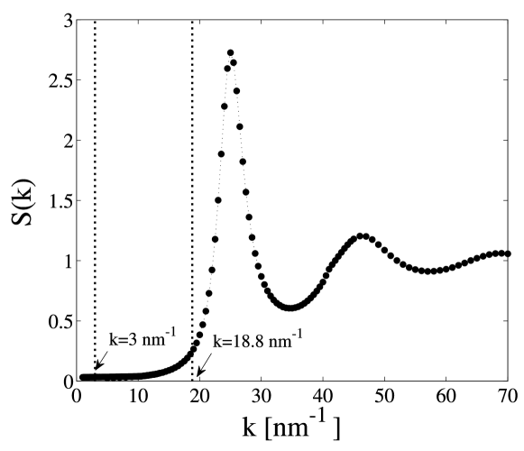
Figure 1: Static structure factor of liquid lithium at the temperature $T=463$ K measured by X-ray diffraction; data taken from Ref. [63]. Two vertical dotted lines mark out the wavenumber range considered in this study. The main peak of the static structure factor $S(k)$ is located at $k_{m}\simeq 24.4$ nm ^-1.

To compare the theoretical classical dynamic structure factor $S(k,\omega)$ with the scattering intensity $I(k,\omega)$, one needs to account for the quantum effects by means of the detailed balance condition

$$S_{q}(k,\omega)=\frac{\hbar\omega/k_{B}T}{1-\exp(-\hbar\omega/k_{B}T)}S(k,\omega),$$ (13uvwamanbhbibjbna)

where $$S_{q}(k,\omega)$$ is the quantum-mechanical structure factor. Then, the experimental resolution effects must be included into consideration through the convolution

$$I(k,\omega)=E(k)\int R(k,\omega-\omega^{\prime})S_{q}(k,\omega^{\prime})d\omega^{\prime},$$ (13uvwamanbhbibjbnb)

where $E(k)$ and $R(k,\omega)$ are the characteristics of the IXS experiment. The quantity $E(k)$ depends on analyzer efficiency and on the atomic form factor [10], whereas $R(k,\omega)$ is the experimental resolution function.

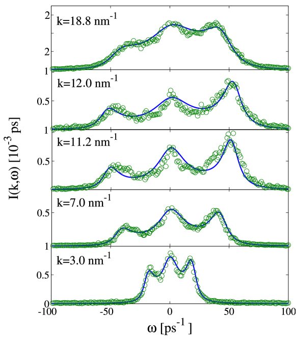
Figure 2: Scattering intensity $I(k,\omega)$ of liquid lithium at the temperature $T=475$ K and several values of the wavenumber $k<k_{m}$, where $k_{m}=24.4$ nm^-1 corresponds to the first peak position of the static structure factor $S(k)$. Open circles ($\circ$) represent experimental IXS data [10], full lines ($-$) depict the theoretical dynamical structure factor $S(k,\omega)$ [see Eq. (13uvwama)] modified to takes into account the quantum-mechanical detailed balance condition and the experimental resolution effects.

Table 1: Values of the frequency parameters $\Delta_{1}^{2}(k)$, $\Delta_{2}^{2}(k)$, $\Delta_{3}^{2}(k)$, $\Delta_{4}^{2}(k)$ (in units of $\times 10^{24}$ s^-2) and values of the coefficients $\mathcal{A}_{1}(k)$ ($\times 10^{26}$ s^-2), $\mathcal{A}_{2}(k)$ ($\times 10^{52}$ s^-4), $\mathcal{A}_{3}(k)$ ($\times 10^{78}$ s^-6) of the polynomial in relation (13uvwama) for the dynamic structure factor $S(k,\omega)$.

• $k$ (nm-1)	$\Delta_{1}^{2}(k)$	$\Delta_{2}^{2}(k)$	$\Delta_{3}^{2}(k)$	$\Delta_{4}^{2}(k)$	$\mathcal{A}_{1}(k)$	$\mathcal{A}_{2}(k)$	$\mathcal{A}_{3}(k)$
  $3.0$	$183\pm 10$	$210\pm 30$	$1500\pm 230$	$17731\pm 4500$	$-6.61$	$11.0$	$4.5$
  $7.0$	$845\pm 30$	$1109\pm 150$	$7110\pm 1350$	$87905\pm 23500$	$-33.78$	$294.8$	$446.2$
  $11.2$	$1346\pm 50$	$1500\pm 220$	$10000\pm 3100$	$179700\pm 43000$	$-52.07$	$681.0$	$1071.8$
  $12.0$	$1545\pm 80$	$1609\pm 240$	$12000\pm 3000$	$157600\pm 40500$	$-54.48$	$729.8$	$2369.9$
  $18.8$	$971\pm 60$	$1589\pm 210$	$11100\pm 2300$	$68540\pm 20000$	$-32.77$	$316.4$	$2027.0$

The dynamic structure factor $S(k,\omega)$ and the scattering intensity $I(k,\omega)$ of liquid lithium at $T=475$ K were defined by means of Eqs. (13uvwama) and Eqs. (13uvwamanbhbibjbna), (13uvwamanbhbibjbnb) at the wavenumbers $k=3.0$, $7.0$, $11.2$, $12.0$ and $18.8$ nm^-1. To determine $S(k,\omega)$ by means of relation (13uvwama) we first need to compute the four frequency parameters $\Delta_{1}^{2}(k)$, $\Delta_{2}^{2}(k)$, $\Delta_{3}^{2}(k)$ and $\Delta_{4}^{2}(k)$. This can be done by two independent methods.

Let us consider the first method used by us to determine these parameters for the case of liquid lithium at the considered thermodynamic state. The frequency parameter $\Delta_{1}^{2}(k)$ has been computed exactly by means of Eq. (13uvwa) [the first equality in this equation] with the experimental values of the static structure factor $S(k)$ from Ref. [63]. The values of the parameter $\Delta_{2}^{2}(k)$ were determined from the first equality of Eq. (13uvw) with the pseudopotential $u(\mathbf{r})$ proposed by Gonzalez et al. [35] and with the radial distribution function $g(r)$ computed on the basis of this potential. It is important to note that the theoretical radial distribution function is consistent with the X-ray diffraction data [63]. Further, although the frequency parameters $\Delta_{3}^{2}(k)$ and $\Delta_{4}^{2}(k)$ can be also computed theoretically through the integral expressions with the three- and four-particle distribution functions [see, for example, Eq. (13uvwc)], this is difficult to implement. Therefore, one can take these two parameters as the fitting parameters. The first way is to calculate the frequency moments $\omega^{(6)}(k)$ and $\omega^{(8)}(k)$ for the experimental spectra of the dynamic structure factor $S(k,\omega)$ [see Eq. (2.1)], and then to find the values of $\Delta_{3}^{2}(k)$ and $\Delta_{4}^{2}(k)$ by means of sum rules (13uvc) and (13uvd).  We have evaluated these parameters, $\Delta_{3}^{2}(k)$ and $\Delta_{4}^{2}(k)$, by a different way. Namely, if one associates the parameter $\Delta_{4}^{2}(k)$ with the correct (experimental) value of $S_{exp}(k,\omega)$ at $\omega=0$ in accordance with relation (13uvwama), i.e.

$$\Delta_{4}^{2}(k)=\left[\frac{\pi S_{exp}(k,\omega=0)}{S(k)}\frac{\Delta_{1}^{2}(k)\Delta_{3}^{2}(k)}{\Delta_{2}^{2}(k)}\right]^{2},$$ (13uvwamanbhbibjbnbo)

then the quantity $\Delta_{3}^{2}(k)$ must be taken directly as fitting parameter. Thus, the two parameters, $\Delta_{3}^{2}(k)$ and $\Delta_{4}^{2}(k)$, are used as adjustable in such the realization of the theoretical model (13uvwama) for $S(k,\omega)$. To our knowledge, there is no other theory for the dynamic structure factor of liquids (even of simple liquids), which operates without fitting parameters, or applies one or two fitting parameters only and yields, herewith, satisfactory agreement with experimental IXS/INS data for the wavenumber range. Further, we recall that the frequency parameters are not the special model parameters, but are the quantities, that determine the sum-rules of the scattering law. Consequently, if the theoretical scheme is capable to reproduce all the features of the scattering law and the scheme satisfies the sum-rules, then theoretical and experimental values of the frequency parameters must be comparable or identical.

The first six frequency parameters, $\Delta_{1}^{2}(k)$, $\Delta_{2}^{2}(k)$, $\Delta_{3}^{2}(k)$, $\Delta_{4}^{2}(k)$, $\Delta_{5}^{2}(k)$ and $\Delta_{6}^{2}(k)$, were also evaluated by means of the second method. In accordance with this method, the configuration data obtained from the simulations with the given interparticle potential $u(\mathbf{r})$ is required only. Then, the frequency moments $\omega^{(j)}(k)$ and the frequency parameters $\Delta_{j}^{2}(k)$ can be determined by means of the original definitions: Eq. (8) with relations (3) and (7). The computational details are given in Appendix. This method yields results for the low-order frequency moments and parameters with high accuracy, that is confirmed by agreement of the results with the data for the experimental static structure factor $S(k)$ and with the exact theoretical values for $\Delta_{1}^{2}(k)$ and $\Delta_{2}^{2}(k)$ evaluated from Eqs. (13uvwa) and (13uvw), respectively. Because of the numerical differentiation procedure used in this method, the magnitude of the statistical error of an evaluated frequency parameter $\Delta_{j}^{2}(k)$ increases with increasing order $j$, where $j=3,\;4,\;5,\;\ldots$. Nevertheless, we find that the values of $\Delta_{3}^{2}(k)$ and $\Delta_{4}^{2}(k)$ agree within the confidence interval with the results obtained from the fitting procedure in accordance with the first method. This confirms that the values of the frequency parameters $\Delta_{1}^{2}(k)$, $\Delta_{2}^{2}(k)$, $\Delta_{3}^{2}(k)$ and $\Delta_{4}^{2}(k)$ obtained by the first method can be adopted; the numerical values of these parameters are given in Tab. 1. The results for the frequency parameters from both the methods will be presented in Fig. 5.

In Fig. 2, the theoretical scattering intensity $I(k,\omega)$ is compared with the experimental IXS data [10]. As seen, the presented theory with expression (13uvwama) for the dynamic structure factor has excellent agreement with experimental data. The theoretical intensity $I(k,\omega)$ accounts for the spectral features. The values of the coefficients $\mathcal{A}_{1}(k)$, $\mathcal{A}_{2}(k)$ and $\mathcal{A}_{3}(k)$ are given in Tab. 1.

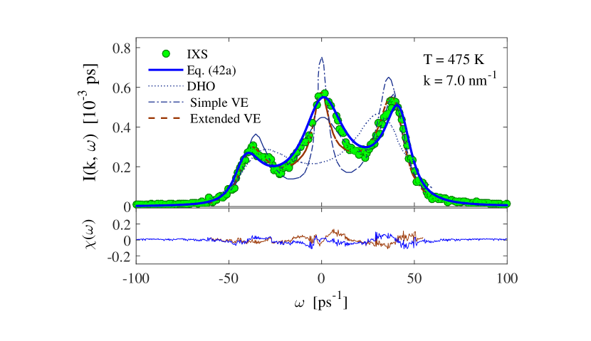
Figure 3: Top: Scattering intensity of liquid lithium at $T=475$ K and $k=7.0$ nm^-1: IXS data (full circles) and results for the DHO model (dotted line), the simple viscoelastic model ($-\cdot-$), the extended viscoelastic model (dashed line) and the results of the theoretical model (13uvwama). IXS data and results for DHO, simple and extended viscoelastic models are taken from Ref. [38]. Bottom: Difference between the experimental data and the theoretical values, $\chi(\omega)=I_{IXS}(k,\omega)-I_{th}(k,\omega)$, computed for the extended viscoelastic model and for the theoretical model  (13uvwama).

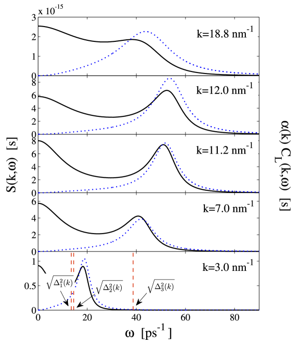
Figure 4: Dynamic structure factor $S(k,\omega)$ (solid line) and scaled longitudinal current correlation function $\alpha(k)C_{L}(k,\omega)$ (dotted line) of liquid lithium at the same temperature and fixed wavenumbers as in Fig. 2. The dimensionless coefficient $\alpha(k)$ takes the values $5\cdot 10^{-5}$, $5\cdot 10^{-5}$, $15\cdot 10^{-5}$, $2\cdot 10^{-4}$, and $3\cdot 10^{-3}$ at $k=3.0$, $7.0$, $11.2$, $12.0$ and $18.8$ nm^-1, respectively. Red vertical dashed lines for the bottom plot correspond to the frequencies $\sqrt{\Delta_{1}^{2}(k)}$, $\sqrt{\Delta_{2}^{2}(k)}$ and $\sqrt{\Delta_{3}^{2}(k)}$ at $k=3.0$ nm^-1.

We note that efficiency of some theoretical models to analyze the same IXS data was verified previously by Scopigno et al. in Ref. [38]. Comparison of experimental data and theoretical results was carried out for the specific spectrum at $k=7.0$ nm^-1. As was clearly demonstrated (Fig. 5 in Ref. [38]), both the damped harmonic oscillator model and the simple viscoelastic model cannot reproduce the lineshape of the scattering intensity. The agreement with the experimental data appears only for the extended viscoelastic model, where the time dependence of the TCF $M_{2}(k,t)$ is approximated by the linear combination of the three exponential decay laws associated with thermal and viscous fluctuations. In Fig. 3, we reproduce all the data from Fig. 5 of Ref. [38] supplemented by our theoretical results. Although the extended viscoelastic model of Ref. [38] and our model with Eq. (13uvwama) do not yield the identical lineshapes of $I(k,\omega)$, both the models are characterized by a comparable agreement with the experimental data. Further, as it was demonstrated in Sec. 3, our theory does not contradict to the extended viscoelastic model and can provide justification for the expansion of the TCF $M_{2}(k,t)$ over exponential functions. For the case of liquid lithium with the estimated frequency parameters $\Delta_{3}^{2}(k)$ and $\Delta_{4}^{2}(k)$ at the considered wavenumbers, we find from Eq. (13uvwamanbf) that the first relaxation time $\tau_{\alpha}(k)$ takes the values from the range $[0.1;1]$ ps, whereas the second relaxation process with $\tau_{\mu}(k)$ occurs over time scales $\sim 0.01$ ps. These estimates are in agreement with results obtained in Refs. [38, 57] with the extended viscoelastic model.

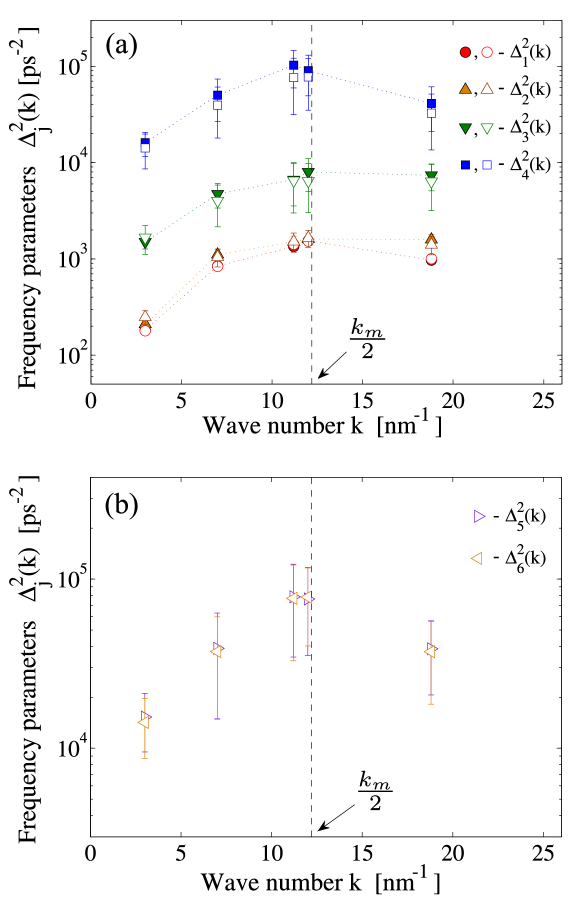
Figure 5: Wavenumber dependence of the frequency parameters $\Delta_{1}^{2}(k)$, $\Delta_{2}^{2}(k)$, $\Delta_{3}^{2}(k)$, $\Delta_{4}^{2}(k)$, $\Delta_{5}^{2}(k)$ and $\Delta_{6}^{2}(k)$ in logarithmic scale. Dashed vertical line corresponds to the wavenumber $k=k_{m}/2\simeq 12.2$ nm ^-1. Full markers correspond to the theoretical values evaluated by the first way (see the text before Eq. (13uvwamanbhbibjbnbo)), whereas transparent markers indicate the values estimated theoretically by the second way – on the basis of Eqs. (7) and (8) with the configuration data (for details, see Appendix).

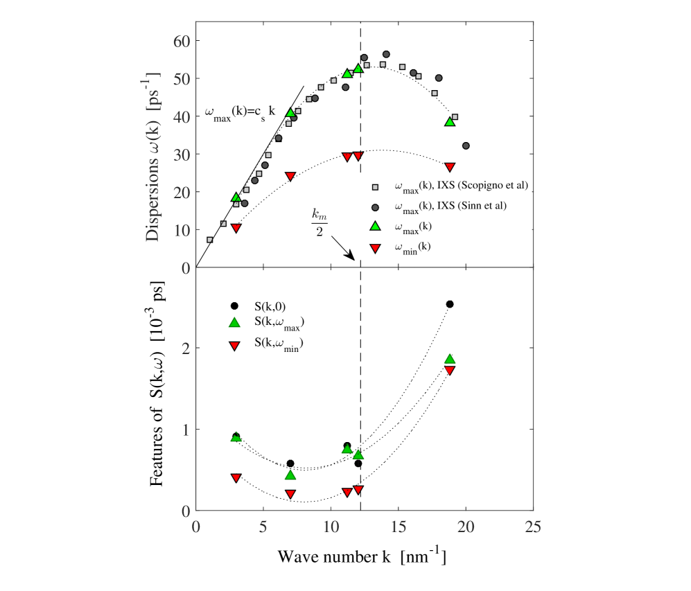
Figure 6: Top: Sound dispersion $\omega_{max}(k)$ and wavenumber-dependent frequency $\omega_{min}(k)$ evaluated from Eqs. (13uvwamanb) and (13uvwamanc); sound dispersions from IXS data of Scopigno et al. [38] (full squares) and Sinn et al. [16] (full circles). Solid line at low wavenumbers corresponds to hydrodynamic frequency of the Mandelshtam-Brillouin doublet $\omega_{c}(k)=c_{s}k$ with the adiabatic sound velocity $c_{s}\simeq 6000$ m/s. Bottom: Wavenumber dependent spectral features: zeroth-frequency spectral component $S(k,\omega=0)$, high-frequency component $S(k,\omega_{max})$, scattering intensity at the minimum $S(k,\omega_{min})$. Dashed vertical line corresponds to the border of the first pseudo-Brillouin zone.

In Fig. 4, the classical dynamic structure factor $S(k,\omega)$ and the longitudinal current correlation function $C_{L}(k,\omega)$ computed on the basis of relations (13uvwama) and (13s) are shown. These results are presented for the same wavenumbers as for the scattering intensity $I(k,\omega)$ in Fig. 2. To make clear correspondence between $S(k,\omega)$ and $C_{L}(k,\omega)$, the spectra of $C_{L}(k,\omega)$ are scaled onto the coefficient $\alpha(k)$. As seen, the high-frequency peak of $S(k,\omega)$ and the peak of $C_{L}(k,\omega)$ are very close, and both the dispersion curves $\omega_{max}(k)$ and $\omega_{c}(k)$ have to be practically identical for the considered wavenumber range [64]. Further, there is no gap between the central component $S(k,\omega=0)$ and the high-frequency component $S(k,\omega_{max})$ as it usually have to be for $S(k,\omega)$ in the hydrodynamic limit (at $k\to 0$) [12]. So, the lineshape of the dynamic structure factor $S(k,\omega)$ at the finite $k$ represents the result of complicated mixing of relaxing and propagative modes. Hence, simple separation of the density fluctuations into two types associated with mechanical processes and with thermal processes is not possible.

The frequency parameters evaluated by means of the two methods are shown in Fig. 5. The wavenumber dependence of these parameters, $\Delta_{1}^{2}(k)$, $\Delta_{2}^{2}(k)$, $\Delta_{3}^{2}(k)$ and $\Delta_{4}^{2}(k)$, are smooth and similar. The parameters increase with increasing wavenumber and saturate at $k\simeq k/k_{m}=12.2$ nm^-1. Then, the frequency parameters start to decrease with further increase of the wavenumber $k$. In fact, the $k$-dependence of the frequency parameters is similar to the dispersion curve $\omega_{max}(k)$ of the acoustic-like excitations in simple liquid [11] [compare with Fig. 6 (top)]. Further, although the parameters $\Delta_{1}^{2}(k)$ and $\Delta_{2}^{2}(k)$ take very close values, nevertheless, the correspondence $\Delta_{j+1}^{2}(k)\geq\Delta_{j}^{2}(k)$ for the frequency parameters $\Delta_{j}^{2}(k)$, $j=1,\;2,\;3,\;4$, still occurs at the considered wavenumbers. The first three frequency parameters take the values corresponding to the square $THz$ frequency scale (or to the inverse square $ps$ timescale). Therefore, these correspond to the typical frequencies of local density fluctuations in a liquid at microscopic spatial scales. The frequency parameter $\Delta_{4}^{2}(k)$ takes the largest values in comparison with $\Delta_{1}^{2}(k)$, $\Delta_{2}^{2}(k)$ and $\Delta_{3}^{2}(k)$. In fact, the parameter $\Delta_{4}^{2}(k)$ defines the upper limit of the frequency domain associated with the density fluctuations. For example, let us consider the dynamic structure factor $S(k,\omega)$ at $k=3.0$ nm^-1 [see the bottom inset in Fig. 4]. Here, the scattering function is completely damped at the frequencies $\omega\geq 30$ ps^-1. The first three frequency parameters are $\Delta_{1}^{2}=183$ ps^-2, $\Delta_{2}^{2}=210$ ps^-2 and $\Delta_{3}^{2}=1500$ ps^-2, whereas the parameter $\Delta_{4}^{2}=177\cdot 10^{2}$ ps^-2 is much larger than $\omega^{2}=900$ ps^-2. One can see from Fig. 5 that both the conditions, $\Delta_{4}^{2}(k)\gg\omega^{2}$ [see also inequality (13uvwad)] and $\Delta_{4}^{2}(k)\approx\Delta_{5}^{2}(k)\approx\Delta_{6}^{2}(k)$ [relation (13uvwae)] are completely supported by obtained values of the frequency parameters. Moreover, there is the following regularity between the frequencies $\sqrt{\Delta_{1}^{2}(k)}$, $\sqrt{\Delta_{2}^{2}(k)}$ and the spectral features of the dynamic structure factor $S(k,\omega)$: both the frequencies $\sqrt{\Delta_{1}^{2}(k)}$ and $\sqrt{\Delta_{2}^{2}(k)}$ are located between the minimum and the high-frequency maximum of $S(k,\omega)$, i.e. within the frequency range $[\omega_{min}(k);\;\omega_{max}(k)]$.

By means of Eqs. (13uvwamanaq), (13uvwamanar) and (13uvwamanas), one can determine the hydrodynamic parameters from the wavenumber dependence of the frequency parameters in the low-$k$ range. We obtain that the sound velocity of liquid lithium at the temperature $T=475$ K is $c_{s}\simeq 6000\pm 1200$ m/s, which is larger than the value $4550$ m/s given in Ref. [15] for liquid lithium at the melting temperature $T_{m}$. Further, our estimates for the thermal diffusivity yield $D_{T}\simeq 21.5\pm 3.5$ nm²/ps. This value is comparable with $19.1$ nm²/ps given for $D_{T}$ of liquid lithium in Ref. [65]. Finally, we find that the sound attenuation coefficient $\Gamma$ takes the value $\simeq 18.4\pm 3.5$ nm²/ps.

Since relation (13uvwama) reproduces the lineshape of the dynamic structure factor $S(k,\omega)$, then all the spectral features can be also recovered. In Fig. 6(top), the frequencies $\omega_{max}(k)$ and $\omega_{min}(k)$ associated with locations of the high-frequency maximum and minimum of $S(k,\omega)$ are presented as functions of the wavenumber $k$. It is necessary to note that the dispersion curve $\omega_{max}(k)$ in the low-$k$ limit must be extrapolated into the hydrodynamic result $\lim_{k\to 0}\omega_{max}(k)=c_{s}k$, whereas $\omega_{min}(k)$ in the low-$k$ asymptotics must be characterized by a gap, which appears because of the separation of the Rayleigh and Brillouin components. It is seen in Fig. 6(bottom) that the evaluated components $S(k,\omega=0)$, $S(k,\omega_{max})$ and $S(k,\omega_{min})$ as functions of the wavenumber are correlated. Namely, the intensities $S(k,0)$ and $S(k,\omega_{min})$ have similar $k-$dependence. Further, the Rayleigh component $S(k,0)$ and the Brillouin component $S(k,\omega_{max})$ take practically the same values for the wavenumbers $k\leq k_{m}/2$ and yield the ratio $S(k,0)/S(k,\omega_{max})\simeq 1$.

5 Concluding remarks

In liquid, overall wavenumber range available for inelastic scattering experiments with photons, neutrons and/or X-rays includes three ranges: the hydrodynamic range (limit), the broad meso-microscopic range and the free-particle dynamics range (limit). An extension of hydrodynamic theory is possible up to such finite wavenumbers, where the hydrodynamic quantities – the viscosity, the thermal conductivity, the sound absorption and others – still have a physical meaning. Let us consider the extended wavenumber range, which includes the wavenumbers corresponding to the hydrodynamic limit and the wavenumbers associated with mesoscopic-microscopic scales. According to the ideas of the generalized hydrodynamics, the viscosity must be transformed into a $k$-dependent parameter when we consider the wavenumbers corresponding to the mesoscopic range. Consequently, at microscopical scales comparable with the size of the second or third pseudo-coordination shells, this macroscopical parameter (the viscosity) must be transformed into a characteristic that takes into account the cumulative result of interparticle interactions within the range. On the other hand, let the wavenumber $k$ decreases from large values associated with the limit of a free moving particle to lower values corresponding to mesoscopic sizes. Here, with decreasing wavenumber, such the characteristic as the thermal velocity of a free moving particle is converted to the phase velocity of the particles enclosed in appropriate spatial range $\ell\sim 2\pi/k$. Thereofore, the theoretical methodology relevant to describe the mesoscopic-microscopic dynamics in liquids has to employ such the quantities as the particle distributions, the interaction energy between the particles and the frequency characteristics of vibration dynamics of a particle with respect to its neighbors (similar to the Einstein frequency).

The theoretical scheme presented in this study exploits the spectral moments of the dynamic structure factor $S(k,\omega)$ and does not apply the assumptions about how many relaxing and propagating modes have to be taken into account. It is important that the spectral moments are determined by the interparticle potential and the structural characteristics. On the other hand, the spectral moments define the sum rules and cannot be considered as arbitrary model parameters. That is important, the presented theoretical scheme satisfies all the sum rules of the scattering law. Moreover, the theoretical relation obtained for the dynamic structure factor $S(k,\omega)$ transforms approximatively at the certain conditions associated with convergence of the high-order frequency parameters to well known hydrodynamic result for $S(k,\omega)$; as well as the theory yields the correct scenario for the high-$k$ limit.

The dynamic structure factor is the characteristic of the longitudinal collective dynamics in liquids [12]. The scattering spectra can also contain marks of the transverse collective excitations with the frequencies lower than $\omega_{c}(k)=c_{s}k$ [66]. However, for the case of an equilibrium simple liquid, the intensity of these excitations is very small and it is barely noticeable in the scattering spectra. In particular, this is evidenced by results of Fig. 2 in Ref. [67], where representation of the scattering spectra in terms of the corresponding longitudinal and transverse components for liquid Fe, Cu and Zn is given. Thus, it is reasonable to overlook the secondary transverse excitations in the analysis of the longitudinal dynamics. Further, according to the theoretical scheme presented in this study, the spectral density of any dynamical variable relevant to the structural relaxation in a liquid can be expressed in terms of its spectral (frequency) moments. Therefore, the presented theory can be directly extended to the case of the transverse collective dynamics.

Alignment of the high-order frequency parameters does not contradict to outcomes the linearized hydrodynamics. In fact, the alignment is identical to the assumption about equality of the TCF’s $M_{3}(k,t)$ and $M_{4}(k,t)$. This allows one to define self-consistently the intermediate scattering function $F(k,t)$ and all other TCF’s: $M_{1}(k,t)$, $M_{2}(k,t)$ and $M_{3}(k,t)$. In such a view, the presented theoretical scheme is similar in its construction to the mode-coupling theories adapted for ergodic systems [44], where the memory function $M_{2}(k,t)$ is expressed in terms of the intermediate scattering function $F(k,t)$. It should be noted that Reichman and Charbonneau [in Ref. [68] (discussion on p. 21)] pointed to a possible extension of the mode-coupling theory, involving the shift of the “mode-coupling closure” to the high-order memory function $M_{4}(k,t)$. This is directly corresponds to the theoretical scheme presented in this study.

In this study, we applied the theoretical approach to determine the dynamic structure factor and the scattering intensity at some selected wavenumbers for the case of liquid lithium. We chose this system to test our theory for the following reasons. As asserted in Ref. [33], the collective microscopic dynamics of this liquid can be more complicated than the dynamics of other liquid metals. Therefore, a microscopic theory may be experiencing difficulties in its application to liquid lithium. On the other hand, there are available the experimental data of the high quality for the microscopic structure and collective dynamics of liquid lithium [36, 16, 38]. We found that the theory is capable of reproducing all the features of the scattering intensity in agreement with IXS data. Finally, the presented theory utilizes the particle interaction potential and structural characteristics as input parameters. Therefore, this theory can be applied directly to the case of any simple fluid.

Appendix: The frequency parameters from configuration data. Details of molecular dynamics simulations

The wavenumber-dependent frequency parameters $\Delta_{1}^{2}(k)$, $\Delta_{2}^{2}(k)$, $\Delta_{3}^{2}(k)$, $\ldots$, can be calculated on the basis of configuration data of the considered many-particle system. These data must include the coordinates, velocities and accelerations, i.e. $\{\mathbf{r}_{1},\;\mathbf{v}_{1},\;\mathbf{a}_{1};\;\mathbf{r}_{2},\;\mathbf{v}_{2},\;\mathbf{a}_{2};\;\ldots;\;\mathbf{r}_{N},\;\mathbf{v}_{N},\;\mathbf{a}_{N}\}$, of all the $N$ particles forming the system, that is usually available, for example, from molecular dynamics simulations with the given interparticle potential. Then, the dynamical variables $A_{0}(k)$, $A_{1}(k)$, $A_{2}(k)$ etc. can be computed on the basis of Eq. (3) and recurrent relation (7), whereas the frequency parameters can be computed from Eq. (8).

In particular, we find for the first five dynamical variables the following exact expressions:

$$A_{0}(k,t)\equiv\rho_{k}(t)=\frac{1}{\sqrt{N}}\sum_{n=1}^{N}\left[\cos(\mathbf{k}\cdot\mathbf{r}_{n}(t))+i\sin(\mathbf{k}\cdot\mathbf{r}_{n}(t))\right],$$ (13uvwamanbhbibjbnbp)

$$A_{1}(k,t)=\frac{1}{\sqrt{N}}\sum_{n=1}^{N}\left[\Bigg{(}\mathbf{k}\cdot\mathbf{v}_{n}(t)\Bigg{)}\Bigg{\{}-\sin(\mathbf{k}\cdot\mathbf{r}_{n}(t))+i\cos(\mathbf{k}\cdot\mathbf{r}_{n}(t))\Bigg{\}}\right],$$ (13uvwamanbhbibjbnbq)

$$A_{2}(k,t) = \frac{1}{\sqrt{N}}\sum_{n=1}^{N}\left[\Bigg{(}\mathbf{k}\cdot\mathbf{a}_{n}(t)\Bigg{)}\Bigg{\{}-\sin(\mathbf{k}\cdot\mathbf{r}_{n}(t))+i\cos(\mathbf{k}\cdot\mathbf{r}_{n}(t))\Bigg{\}}\right.$$ (13uvwamanbhbibjbnbr)

$$\left.+\Bigg{(}\mathbf{k}\cdot\mathbf{v}_{n}(t)\Bigg{)}^{2}\Bigg{\{}-\cos(\mathbf{k}\cdot\mathbf{r}_{n}(t))-i\sin(\mathbf{k}\cdot\mathbf{r}_{n}(t))\Bigg{\}}\right]$$

$$+ \Delta_{1}^{2}(k)A_{0}(k,t),$$

$$A_{3}(k,t) = \frac{1}{\sqrt{N}}\sum_{n=1}^{N}\left[\Bigg{(}\mathbf{k}\cdot\frac{d\mathbf{a}_{n}(t)}{dt}\Bigg{)}\Bigg{\{}-\sin(\mathbf{k}\cdot\mathbf{r}_{n}(t))+i\cos(\mathbf{k}\cdot\mathbf{r}_{n}(t))\Bigg{\}}\right.$$ (13uvwamanbhbibjbnbs)

$$\left.+\Bigg{(}\mathbf{k}\cdot\mathbf{v}_{n}(t)\Bigg{)}^{3}\Bigg{\{}\sin(\mathbf{k}\cdot\mathbf{r}_{n}(t))-i\cos(\mathbf{k}\cdot\mathbf{r}_{n}(t))\Bigg{\}}\right.$$

$$\left.+3\Bigg{(}\mathbf{k}\cdot\mathbf{v}_{n}(t)\Bigg{)}\Bigg{(}\mathbf{k}\cdot\mathbf{a}_{n}(t)\Bigg{)}\Bigg{\{}-\cos(\mathbf{k}\cdot\mathbf{r}_{n}(t))-i\sin(\mathbf{k}\cdot\mathbf{r}_{n}(t))\Bigg{\}}\right]$$

$$+ \left[\Delta_{1}^{2}(k)+\Delta_{2}^{2}(k)\right]A_{1}(k,t)$$

and

$$A_{4}(k,t) = \frac{1}{\sqrt{N}}\sum_{n=1}^{N}\left[\Bigg{(}\mathbf{k}\cdot\frac{d^{2}\mathbf{a}_{n}(t)}{dt^{2}}\Bigg{)}\Bigg{\{}-\sin(\mathbf{k}\cdot\mathbf{r}_{n}(t))+i\cos(\mathbf{k}\cdot\mathbf{r}_{n}(t))\Bigg{\}}\right.$$ (13uvwamanbhbibjbnbt)

$$\left.+4\Bigg{(}\mathbf{k}\cdot\mathbf{v}_{n}(t)\Bigg{)}\Bigg{(}\mathbf{k}\cdot\frac{d\mathbf{a}_{n}(t)}{dt}\Bigg{)}\Bigg{\{}-\cos(\mathbf{k}\cdot\mathbf{r}_{n}(t))-i\sin(\mathbf{k}\cdot\mathbf{r}_{n}(t))\Bigg{\}}\right.$$

$$\left.+3\Bigg{(}\mathbf{k}\cdot\mathbf{a}_{n}(t)\Bigg{)}^{2}\Bigg{\{}-\cos(\mathbf{k}\cdot\mathbf{r}_{n}(t))-i\sin(\mathbf{k}\cdot\mathbf{r}_{n}(t))\Bigg{\}}\right.$$

$$\left.+6\Bigg{(}\mathbf{k}\cdot\mathbf{v}_{n}(t)\Bigg{)}^{2}\Bigg{(}\mathbf{k}\cdot\mathbf{a}_{n}(t)\Bigg{)}\Bigg{\{}\sin(\mathbf{k}\cdot\mathbf{r}_{n}(t))-i\cos(\mathbf{k}\cdot\mathbf{r}_{n}(t))\Bigg{\}}\right.$$

$$\left.+\Bigg{(}\mathbf{k}\cdot\mathbf{v}_{n}(t)\Bigg{)}^{4}\Bigg{\{}\cos(\mathbf{k}\cdot\mathbf{r}_{n}(t))+i\sin(\mathbf{k}\cdot\mathbf{r}_{n}(t))\Bigg{\}}\right]$$

$$+ \Bigg{(}\Delta_{1}^{2}(k)+\Delta_{2}^{2}(k)+\Delta_{3}^{2}(k)\Bigg{)}\Bigg{(}A_{2}(k,t)-\Delta_{1}^{2}(k)A_{0}(k,t)\Bigg{)}$$

$$+ \Delta_{1}^{2}(k)\Delta_{3}^{2}(k)A_{0}(k,t).$$

The time derivatives $d\mathbf{a}_{n}(t)/dt$ and $d^{2}\mathbf{a}_{n}(t)/dt^{2}$ in Eqs. (13uvwamanbhbibjbnbs) and (13uvwamanbhbibjbnbt) can be determined numerically by the finite difference method. Namely, one can apply the next simple scheme:

$$\frac{d\mathbf{a}_{n}(t_{i+1})}{dt}=\lim_{\Delta t\rightarrow 0}\frac{\mathbf{a}_{n}(t_{i+1})-\mathbf{a}_{n}(t_{i})}{\Delta t},$$ (13uvwamanbhbibjbnbu)

$$\frac{d^{2}\mathbf{a}_{n}(t_{i+2})}{dt^{2}}=\lim_{\Delta t\rightarrow 0}\frac{\mathbf{a}_{n}(t_{i+2})-2\mathbf{a}_{n}(t_{i+1})+\mathbf{a}_{n}(t_{i})}{\Delta t},$$ (13uvwamanbhbibjbnbv)

with the simulation time step $\Delta t=1\,$fs and $i=1,\,2,\,3,\,...$. Further, by applying relation (7), one can obtain expressions for the dynamical variables of a higher order. Then, Eq. (8) can be rewritten in the form adapted for the numerical estimation of the frequency parameters:

$$\Delta_{j+1}^{2}(k)=\frac{\left\langle\left\{\mathrm{Re}[A_{j+1}(k,t)]\right\}^{2}+\left\{\mathrm{Im}[A_{j+1}(k,t)]\right\}^{2}\right\rangle}{\left\langle\left\{\mathrm{Re}[A_{j}(k,t)]\right\}^{2}+\left\{\mathrm{Im}[A_{j}(k,t)]\right\}^{2}\right\rangle},$$ (13uvwamanbhbibjbnbw)

$$j=1,\;2,\;3,\ldots.$$

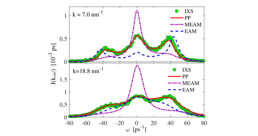
Figure 7: Scattering intensity of liquid lithium at the temperature $T=475$ K and at the selected wavenumbers. Comparison experimental IXS data [38] and results of MD simulations with the model pseudopotential [35], with the EAM potential [69] and with the MEAM potential [70].

For the case of the isotropic equilibrium system, the ensemble average in Eq. (13uvwamanbhbibjbnbw) is realized by means of the averaging over configurations at different time moments and averaging over different directions of the wavevector $\mathbf{k}$ at the fixed

$$k=|\mathbf{k}|=\sqrt{k_{x}^{2}+k_{y}^{2}+k_{z}^{2}}$$

within the given geometry of the simulation box.

Note that we have verified the various model potentials suggested for liquid lithium. It is remarkable that the pseudopotential proposed by Gonzalez et al. yields very good agreement with X-ray diffraction data for the structure properties and excellent agreement with IXS data for the dynamical properties [37]. In particular, the scattering intensity $I(k,\omega)$ calculated with this pseudopotential reproduces the experimental data with a higher accuracy than the scattering intensity obtained with the EAM [69] and MEAM potentials [70] (see Fig. 7). Therefore, we have used this pseudopotential to generate the configuration data and, then, to estimate the frequency parameters.

Thus, the first six frequency parameters $\Delta_{1}^{2}(k)$, $\Delta_{2}^{2}(k)$, …, $\Delta_{6}^{2}(k)$ of the liquid lithium for the considered wavenumber range were calculated on the basis of molecular dynamics simulation data for the system of $N=16\;000$ particles interacted through the effective pseudopotential suggested by Gonzalez et al. [35]. It was employed the cubic simulation box ($L_{x}=L_{y}=L_{z}=6.98\,$nm) with the periodic boundary conditions in all the directions. The values of the frequency parameters were also averaged over data of independent simulations runs. The obtained values of these parameters are presented in Fig. 5.

References

References

- [1] Resibois P and de Leener M 1977 Classical Kinetic Theory of Fluids (New York: Wiley)
- [2] Landau L D and Placzek G 1934 Phys. Z. Sowjun. 5 172
- [3] Price D L, Saboungi M-L, Bermejo F J 2003 Rep. Prog. Phys. 66 407
- [4] Verkerk P 2001 J. Phys.: Condens. Matter 13 7775
- [5] Copley J R D, Lovesey S W 1975 Rep. Prog. Phys. 38 461
- [6] de Gennes P G 1959 Physica 25 825
- [7] Montfrooij W 2016 J. Non-Cryst. Solids 445-446 15
- [8] Hansen J P, McDonald I R 2006 Theory of Simple Liquids (London: Academic Press)
- [9] Balucani U and Zoppi M 1994 Dynamics of the Liquid State (Oxford: Clarendon Press)
- [10] Scopigno T, Ruocco G, Sette F 2005 Rev. Mod. Phys. 77 881
- [11] Pilgrim W-C, Morkel Chr 2006 J. Phys.: Condens. Matter 18 R585
- [12] Egelstaff P A 1965 Thermal Neutron Scattering (New York: Academic Press)
- [13] Götze W 1989 “Aspects of structural glass transitions”, in Liquids, Freezing and the Glass Transition ed J P Hansen, D Levesque and J Zinn-Justin (North-Holland, Amsterdam)
- [14] Boon J P and Yip S 1991 Molecular Hydrodynamics (New York: Dover Publ.)
- [15] Ohse R 1985 Handbook of Thermodynamic and Transport Properties of Alkali Metals (Blackwell Scientific Publications)
- [16] Sinn H, Sette F, Bergmann U, Halcoussis Ch, Krisch M, Verbeni R and Burkel E 1997 Phys. Rev. Lett. 78 1715
- [17] Novikov A, Savostin V, Shimkevich A, Yulmetyev R, Yulmetyev T 1996 Physica B: Cond. Matter 228 312
- [18] Copley J R D and Rowe M 1974 Phys. Rev. A 9 1656
- [19] Bodensteiner T, Morkel C, Gläser W and Dorner B 1992 Phys. Rev. A 45 5709
- [20] Giordano V M, Monaco G 2009 Phys. Rev. B 79 020201(R)
- [21] Cabrillo C, Bermejo F J, Alvarez M, Verkerk P, Maira-Vidal A, Bennington S M and Martín D 2002 Phys. Rev. Lett. 89 075508
- [22] Torcini A, Balucani U, de Jong P H K, Verkerk P 1995 Phys. Rev. E 51 3126
- [23] Casas J, González D J, González L E, Alemany M M G, Gallego L J 2000 Phys. Rev. B 62 12095
- [24] Canales M, González L E, Padró J A 1994 Phys. Rev. E 50 3656
- [25] Gonzalez D J, González L E, Hoshino K 1994 J. Phys.: Condens. Matter 6 3849
- [26] Yulmetyev R M, Mokshin A V, Hänggi P and Shurygin V Yu 2001 Phys. Rev. E 64 057101
- [27] Yulmetyev R M, Mokshin A V, Hänggi P and Shurygin V Yu 2002 JETP Letters 76 147
- [28] Yulmetyev R M, Mokshin A V, Scopigno T and Hänggi P 2003 J. Phys.: Codens. Matter 15 2235
- [29] Mokshin A V, Yulmetyev R M, Hänggi P 2004 J. Chem. Phys. 121 7341
- [30] Mokshin A V, Yulmetyev R M, Khusnutdinov R M, Hänggi P 2006 JETP 103 841
- [31] Anta J A and Madden P A 1999 J. Phys.: Condens. Matter 11 6099
- [32] Mokshin A V, Yulmetyev R M, Khusnutdinoff R M, Hänggi P 2007 J. Phys.: Condens. Matter 19 046209
- [33] Singh S, Sood J, Tankeshwar K 2007 J. Non-Cryst. Solids 353 3134
- [34] Kresse G 1996 J. Non-Cryst. Solids 205-207 833
- [35] Gonzalez L E, Gonzalez D J, Lopez J M 2001 J. Phys.: Condens. Matter 13 7801
- [36] Salmon P S, Petri I, de Jong P H K, Verkerk P, Fisher H E, Howells W S 2004 J. Phys.: Condens. Matter 16 195
- [37] Khusnutdinoff R M, Galimzyanov B N, Mokshin A V 2018 JETP (accepted)
- [38] Scopigno T, Balucani U, Ruocco G, Sette F 2000 J. Phys.: Condens. Matter 12 8009
- [39] Singh Sh, Tankeswar K 2003 Phys. Rev. E 67 012201
- [40] Zwanzig R 2001 Nonequilibrium statistical mechanics (Oxford: Clarendon Press)
- [41] Balucani U, Lee M H, Tognetti V 2003 Phys. Rep. 373 409
- [42] Lee M H 2000 Phys. Rev. E 62 1769
- [43] Mokshin A V 2015 Theoretical and Mathematical Physics 183 449
- [44] Götze W 2009 Complex Dynamics of Glass-Forming liquids (Oxford: Oxford University Press).
- [45] Vorberger J, Donko Z, Tkachenko I M, Gericke D O 2012 Phys. Rev. Lett. 109 225001
- [46] Arkhipov Yu V, Ashikbayeva A B, Askaruly A and Davletov A E, Tkachenko I M 2014 Phys. Rev. E 90 053102
- [47] Bhalla P, Dasa N, Singha N 2016 Physica A: Statistical Mechanics and its Applications 380 2000
- [48] Yu Ming B 2016 Physica A: Statistical Mechanics and its Applications 447 411
- [49] Wierling A, Sawada I 2010 Phys. Rev. E 82 051107
- [50] Khusnutdinoff R M, Mokshin A V, Klumov B A, Ryltsev R E, Chtchelkatchev N M 2016 JETP 123 265
- [51] Chtchelkatchev N M, Klumov B A, Ryltsev R E, Khusnutdinov R M, Mokshin A V 2016 JETP Letters 103 390
- [52] Mokshin A V, Yulmetyev R M, Hänggi P 2005 Phys. Rev. Lett. 95 200601
- [53] Yoshido F, Takeno S 1989 Phys. Rep. 173 301
- [54] Mountain R D 1966 Rev. Mod. Phys. 38 205
- [55] Verkerk P, De-Jong P H K, Arai M, Bennington S M, Howells W S, Taylor A D 1992 Physica B 180-181 834
- [56] Burkel E, Sinn H 1994 J. Phys.: Condens. Matter 6 A225
- [57] Scopigno T, Balucani U, Ruocco G, Sette F 2000 Phys. Rev. Lett. 85 4076
- [58] Aliotta F, Gapiński J, Pochylski M, Ponterio R C, Saija F, Vasi C 2011 Phys. Rev. E 84 051202
- [59] Bafile U, Guarini E, Barocchi F 2006 Phys. Rev. E 73 061203
- [60] Hosokawa S, Pilgrim W-C, Kawakita Y, Ohshima K, Takeda S, Ishikawa D, Tsutsui S, Tanaka Y and Baron A Q R 2003 J. Phys.: Condens. Matter 15 L623
- [61] Hosokawa S, Kawakita Y, Pilgrim W-C, Sinn H 2001 Phys. Rev. B 63 134205
- [62] Bove L E, Sacchetti F, Petrillo C, Dorner B, Formisano F, Sampoli M, Barocchi F 2002 J. Non-Cryst. Solids 307-310 842
- [63] Waseda Y 1980 The Structure of Non-crystalline Materials: Liquids and Amorphous Solids (New-York: McGraw-Hill)
- [64] Fomin Yu D, Ryzhov V N, Tsiok E N, Brazhkin V V, Trachenko K 2016 J. Phys.: Condens. Matter 28 43LT01
- [65] Touioukiam Y, Ho C 1973 Thermal Diffusivity, Vol. 10 Thermophysical Properties of Matter (IFI-Plenum, New York).
- [66] Giordano V M, Monaco G 2010 PNAS 107 21985
- [67] Hosokawa S, Inui M, Kajhara Y, Tsutsui S, Baron A Q R 2015 J. Phys.: Condens. Matter 27 194104
- [68] Reichman D R, Charbonneau P 2005 J. Stat. Mech. P05013
- [69] Belashchenko D K 2012 Inorg. Mater. 48 79
- [70] Baskes M I 1992 Phys. Rev. B 46 2727