Automated Calculation of Dijet Soft Functions
in the Presence of Jet Clustering Effects

Abstract:

We extend our framework for the automated calculation of dijet soft functions to observables that do not obey the non-Abelian exponentiation theorem, like jet-veto or grooming soft functions that are sensitive to clustering effects of the jet algorithm. Although the matrix element for uncorrelated double emissions has a simpler structure than the one for correlated emissions, we argue that its singularity structure poses more stringent constraints on the required phase-space parametrisation. Our algorithm applies to both SCET-1 and SCET-2 soft functions and it is implemented in the novel program SoftSERVE. We present results for various jet-veto observables and obtain new predictions for the soft-drop jet-grooming algorithm.

1 Introduction

In this contribution we report on progress in our effort to automate the calculation of dijet soft functions to next-to-next-to-leading order (NNLO) accuracy. The general idea of our framework was introduced in [1], to which we refer for most of the definitions that are used in this article. The extensions with respect to [1] are threefold: (i) We relax the assumption that the observable should be consistent with the non-Abelian exponentiation (NAE) theorem. (ii) The formalism is extended to soft functions that are relevant for transverse-momentum resummation (so-called SCET-2 observables). (iii) We introduce the program SoftSERVE, which allows for an efficient numerical evaluation of soft functions that are defined in terms of two back-to-back light-like Wilson lines. We briefly address each of these points in the following, before presenting sample results for jet-veto and jet-grooming soft functions.

2 Uncorrelated emissions

The soft functions we consider are of the form

$$S(\tau,\mu)=\frac{1}{N_{c}}\;\sum_{X}\;\mathcal{M}(\tau;\{k_{i}\})\;\mathrm{Tr}\;\langle 0|S^{\dagger}_{\bar{n}}S_{n}|X\rangle\langle X|S^{\dagger}_{n}S_{\bar{n}}|0\rangle\,,$$ (1)

where $S_{n}$ and $S_{\bar{n}}$ are soft Wilson lines in the fundamental colour representation. Up to NNLO it is irrelevant whether the light-like vectors $n^{\mu}$ and $\bar{n}^{\mu}$ (which are normalised to $n\cdot\bar{n}=2$) correspond to incoming or outgoing directions [2, 3]. Our results therefore equally apply to $e^{+}e^{-}$ dijet observables, one-jet observables in deep-inelastic scattering or zero-jet observables at hadron colliders. For simplicity, we refer to all of these cases as dijet soft functions in the following.

The definition involves a generic measurement function $\mathcal{M}(\tau,\{k_{i}\})$ that provides a constraint on the soft radiation with parton momenta $\{k_{i}\}$ according to the observable under consideration. The explicit form we assume for the single-emission measurement function was given in [1]. It depends on the Laplace variable $\tau$ (of dimension 1/mass) and a function $f(y,\theta)$ that encodes the angular and rapidity dependence of the observable. In our approach, it is crucial that this function is finite and non-zero in the limits in which the corresponding matrix element becomes singular. We therefore factor out an appropriate power of the rapidity variable $y$ that is controlled by a parameter $n$ (see [1] for details).

At NNLO the double real-emission contribution consists of three colour structures: $C_{F}C_{A}$, $C_{F}T_{F}n_{f}$ and $C_{F}^{2}$. The parametrisation of the measurement function for the first two structures (the so-called correlated-emission contribution) was specified in [1]. For the remaining colour structure, we start from

$$S_{2}^{RR}(\epsilon)=\frac{(4\pi e^{\gamma_{E}}\tau^{2})^{-2\epsilon}}{(2\pi)^{2d-2}}\,\int d^{d}k\;\,\delta(k^{2})\,\theta(k^{0})\,\int d^{d}l\;\,\delta(l^{2})\,\theta(l^{0})\;\mathcal{M}(\tau;k,l)\,|\mathcal{A}_{RR}(k,l)|^{2}$$ (2)

in dimensional regularisation with $d=4-2\epsilon$. The matrix element of the uncorrelated-emission contribution is particularly simple,

$$|\mathcal{A}_{RR}(k,l)|^{2}=\frac{2048\pi^{4}\,C_{F}^{2}}{k_{+}k_{-}l_{+}l_{-}}\,.$$ (3)

In [1] we assumed that the measurement function was consistent with the NAE theorem [4, 5] and the uncorrelated-emission contribution was therefore proportional to the square of the NLO correction. We relax this assumption in this work and compute this contribution explicitly. To this end, we need to find a phase-space parametrisation that disentangles the singularity structure of the matrix element and that allows us to control the measurement function in its singular limits (in the same sense that the NLO function $f(y,\theta)$ has to be finite and non-zero as $y\to 0$). It turns out that the latter requirement necessarily introduces non-trivial correlations between the parton momenta $k$ and $l$. Our parametrisation for the uncorrelated-emission contribution,

$$q_{T} =\sqrt{k_{+}k_{-}}\left(\frac{\sqrt{l_{+}l_{-}}}{l_{-}+l_{+}}\right)^{-n}+\sqrt{l_{+}l_{-}}\left(\frac{\sqrt{k_{+}k_{-}}}{k_{-}+k_{+}}\right)^{-n},\hskip 28.45274pty_{k}=\frac{k_{+}}{k_{-}}\,,\qquad$$

$$b =\sqrt{\frac{k_{+}k_{-}}{l_{+}l_{-}}}\left(\frac{\sqrt{k_{+}k_{-}}}{k_{-}+k_{+}}\right)^{n}\left(\frac{\sqrt{l_{+}l_{-}}}{l_{-}+l_{+}}\right)^{-n},\hskip 76.82234pty_{l}=\frac{l_{+}}{l_{-}}\,,$$ (4)

is therefore more complicated than the one we used for the correlated emissions (see [1]). Notice that this parametrisation depends on the parameter $n$, i.e. it is strictly speaking not observable-independent. In physical terms, the variables $y_{k}$ and $y_{l}$ are measures of the rapidities of the individual partons, whereas $b$ and $q_{T}$ reduce for $n=0$ to the ratio and the scalar sum of their transverse momenta, respectively (the parentheses introduce rapidity-dependent weight factors for $n\neq 0$). The measurement function for the uncorrelated emission contribution is then parametrised as

$$\mathcal{M}(\tau;k,l)=\exp\big{(}-\tau\,q_{T}\,y_{k}^{n/2}\,y_{l}^{n/2}\,G(y_{k},y_{l},b,\theta_{k},\theta_{l},\theta_{kl})\big{)}\,,$$ (5)

where $\theta_{k}$, $\theta_{l}$ and $\theta_{kl}$ are angular variables that were defined in [1]. The linear dependence on $q_{T}$ is fixed on dimensional grounds, and the factors $y_{k}^{n/2}$ and $y_{l}^{n/2}$ are required to make the function $G(y_{k},y_{l},b,\theta_{k},\theta_{l},\theta_{kl})$ finite and non-zero in the collinear limits $y_{k}\to 0$ and $y_{l}\to 0$. As an example, we quote the measurement function for $W$-production at large transverse momentum [6],

$$G(y_{k},y_{l},b,\theta_{k},\theta_{l},\theta_{kl})=\frac{b(1+y_{l})}{(1+b)}\,\big{(}1+y_{k}-2\sqrt{y_{k}}\,\cos\theta_{k}\big{)}+\frac{(1+y_{k})}{(1+b)}\,\big{(}1+y_{l}-2\sqrt{y_{l}}\,\cos\theta_{l}\big{)}\,.$$ (6)

Similar to the correlated-emission contribution, the measurement function satisfies non-trivial constraints from infrared-collinear safety,

$$G(y_{k},y_{l},0,\theta_{k},\theta_{l},\theta_{kl})=\frac{f(y_{l},\theta_{l})}{(1+y_{k})^{n}}\,,\qquad\qquad G(y_{l},y_{l},b,\theta_{l},\theta_{l},0)=\frac{f(y_{l},\theta_{l})}{(1+y_{l})^{n}}\,,$$ (7)

which correspond to the soft limit $k^{\mu}\to 0$ and the collinear limit $k^{\mu}\propto l^{\mu}$, respectively. We further exploit the symmetries from $n\leftrightarrow\bar{n}$ and $k\leftrightarrow l$ exchange to map the integration region onto the unit hypercube. For the jet algorithms we have considered so far, it is also crucial to disentangle the scalings of the measurement function in the joint limit $y_{k}\to 0$ and $y_{l}\to 0$ at a fixed ratio $r=y_{k}/y_{l}$ from the one of the subsequent limits with $r\to 0$. In total we are then left with a six-dimensional integral representation of the uncorrelated-emission contribution, which contains an explicit singularity from the limit $q_{T}\to 0$ and implicit divergences from $y_{k}\to 0$, $r\to 0$ and $b\to 0$. The $C_{F}^{2}$ contribution thus starts with a $1/\epsilon^{4}$ pole.

3 SCET-2 and collinear anomaly

The algorithm we have outlined so far leads to rapidity integrals of the form $\int_{0}^{1}dy\;\,y^{-1+n\epsilon}$, which are not regularised for $n=0$. This particular case corresponds to a SCET-2 observable, which are known to require an additional regulator on top of dimensional regularisation. Here we follow the strategy proposed in [7] and implement the regulator on the level of the phase-space integrals. In order to keep the $n\leftrightarrow\bar{n}$ symmetry, we write the generic phase-space measure as

$$\int\!d^{d}p\;\left(\frac{\nu}{p_{+}+p_{-}}\right)^{\alpha}\;\delta(p^{2})\theta(p^{0})\,,$$ (8)

and the rapidity divergences then manifest themselves as poles in the regulator $\alpha$.

The $1/\alpha$ poles induce logarithmic corrections in the rapidity scale $\nu$, which are controlled by the collinear anomaly exponent $F$,

$$S(\tau,\mu,\nu) =(\nu^{2}\bar{\tau}^{2})^{-F(\tau,\mu)}\;W_{S}(\tau,\mu)\,,$$ (9)

where $\bar{\tau}=\tau e^{\gamma_{E}}$ and the soft remainder function $W_{S}$ contains the finite terms in the $\alpha$-expansion. From the calculation of the bare soft function, one can thus determine the bare collinear anomaly exponent $F_{0}$, which renormalises additively in Laplace space, $F_{0}=F+Z_{F}$. The renormalised anomaly exponent $F$ fulfills a renormalisation group (RG) equation

$$\frac{\mathrm{d}}{\mathrm{d}\ln\mu}\;F(\tau,\mu) =2\,\Gamma_{\mathrm{cusp}}(\alpha_{s})\,,$$ (10)

which is governed by the cusp anomalous dimension. Expanding $\Gamma_{\mathrm{cusp}}(\alpha_{s})=\sum_{n=0}^{\infty}\,\Gamma_{n}(\frac{\alpha_{s}}{4\pi})^{n+1}$, the two-loop solution of the RG equation takes the form

$$F(\tau,\mu) =\left(\frac{\alpha_{s}}{4\pi}\right)\Big{\{}2\Gamma_{0}\,L+d_{1}\Big{\}}+\left(\frac{\alpha_{s}}{4\pi}\right)^{2}\Big{\{}2\beta_{0}\Gamma_{0}\,L^{2}+2\left(\Gamma_{1}+\beta_{0}d_{1}\right)L+d_{2}\Big{\}}$$ (11)

with $L=\ln(\mu\bar{\tau})$. Explicit expressions of the expansion coefficients $\Gamma_{0}$ and $\Gamma_{1}$ as well as the beta-function coefficient $\beta_{0}$ can be found in [1].

The $Z$-factor $Z_{F}$ satisfies a similar RG equation as the anomaly exponent and its explicit form to two-loop order is given by

$$Z_{F} =\left(\frac{\alpha_{s}}{4\pi}\right)\left\{\frac{\Gamma_{0}}{\epsilon}\right\}+\left(\frac{\alpha_{s}}{4\pi}\right)^{2}\bigg{\{}-\frac{\beta_{0}\Gamma_{0}}{2\epsilon^{2}}+\frac{\Gamma_{1}}{2\epsilon}\bigg{\}}\,.$$ (12)

The cancellation of the divergences $1/\epsilon^{j}$ with $j=1,2$ in the renormalised anomaly exponent $F$ provides a strong check of our calculation. The finite terms, on the other hand, determine the one-loop and two-loop anomaly coefficients $d_{1}$ and $d_{2}$. The extraction of $d_{2}$ from the bare soft function is actually subtle since the one-particle and two-particle cuts have different scalings in the rapidity scale $\nu$. The coefficients of the $1/\alpha$ pole terms and the associated logarithms in the rapidity scale $\nu$ are therefore different; see the discussion in section 4.3 of [8] for more details.

4 Numerical implementation

The integral representations that we have derived above and in [1] are implemented in the custom C++ program SoftSERVE. In [1] we found an overlapping divergence in the correlated-emission contribution (in the limits $a\to 1$ and $t_{kl}\to 0$), which we could resolve in the meantime by an additional substitution. In other words, all singularities are factorised in the applied formulae and no sector decomposition strategy is needed anymore to disentangle the divergences.

With all singularities factorised in the form $x^{-1+m\epsilon+k\alpha}$, they can easily be made explicit by introducing standard plus-distributions. One must further respect the ordering of the $\alpha$- and $\epsilon$-expansions, since the additional regulator should only be used to regularize rapidity divergences for SCET-2 soft functions. As the measurement functions $f$, $F$ and $G$ are by construction finite and non-zero in the singular limits (and independent of the regulators), they can be kept symbolic during the subtraction and expansion steps, and their explicit forms are only resolved at the final numerical integration stage.

For the numerical integrations SoftSERVE applies the Divonne integrator of the Cuba library [9]. The code contains a number of further refinements to improve the convergence of the numerical integrations (for more details, see [10]). In particular, we eliminated all (integrable) square-root divergences with appropriate remappings in order to obtain a more reliable error estimate for the Monte Carlo integrations. For some of the observables, we observed large cancellations between different terms, which could not be resolved with double precision variables. We therefore implemented an option to work with multi-precision variables provided by the boost [11] and GMP/MPFR [12] libraries, although this option significantly slows down the program.

Leaving the last issue aside, a typical SoftSERVE run usually takes less than half an hour on a standard quad-core machine to determine a bare NNLO soft function up to the finite terms to 3-4 digits precision. As the Cuba integrators support parallelisation, it is possible to increase the precision to a few more digits on a reasonable time scale. In addition, SoftSERVE provides scripts for the renormalisation of bare soft functions in both Laplace and cumulant space; further details will be given in a future publication [13].

We checked our results with an independent code that uses the public programs SecDec ​​​3 [14] and pySecDec [15]. As the new python-based version of SecDec supports an arbitrary number of analytic regulators, it is particularly suited for SCET-2 problems. For the numerical integrations in SecDec we used the Cuba integrators Suave and Vegas for independent cross checks.

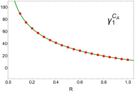
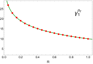
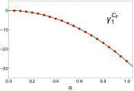
Figure 1: Two-loop anomalous dimension of the rapidity-dependent jet-veto soft functions from [16]. The (red) dots represent our SoftSERVE numbers and the solid (green) lines are the fit functions that were obtained in [17].

5 Results

In this article we focus on jet-veto and jet-grooming observables. For SCET-1 soft functions with $n\neq 0$, we present results for the two-loop anomalous dimension $\gamma_{1}^{S}$ that was defined in [1]. For observables that violate the NAE theorem, the anomalous dimension has three colour structures,

$$\gamma_{1}^{S} =\gamma_{1}^{C_{A}}\;C_{F}C_{A}+\gamma_{1}^{n_{f}}\;C_{F}T_{F}n_{f}+\gamma_{1}^{C_{F}}\;C_{F}^{2}\,,$$ (13)

of which $\gamma_{1}^{C_{A}}$ and $\gamma_{1}^{n_{f}}$ can be calculated with the strategy from [1]. The NAE-violating coefficient $\gamma_{1}^{C_{F}}$, on the other hand, can be determined with the novel method that we discussed in Section 2.

We first consider the rapidity-dependent jet-veto observables that were introduced in [16]. As the RG equation for these observables holds in cumulant rather than Laplace space, we have to take the Laplace transform of the respective soft functions to bring them into the form that we assume for the measurement function. It is then possible to correct for the factors associated with the inversion of the Laplace transformation on the level of the bare soft functions.

For the one-loop soft anomalous dimension, the integrals can be solved analytically and one finds $\gamma_{0}^{S}=0$. At two-loop order, we have evaluated the soft functions with SoftSERVE for 20 values of the jet radius $R$ between $R=0.05$ and $R=1$. Our results are displayed in Figure 1, which also shows fitting functions that were obtained in a previous calculation [17]. Our results nicely agree with these functions and they represent the first confirmation of the calculation in [17].

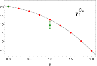
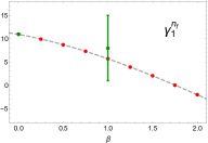
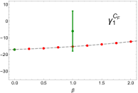
Figure 2: Two-loop anomalous dimension of the soft-drop jet-grooming soft function from [18]. The (red) dots represent our SoftSERVE numbers and the dashed lines are interpolating functions of our results. The (green) dots with error bars are the numbers from [18].

We next turn to the soft-drop jet-grooming soft function that was discussed in [18]. This function also renormalises multiplicatively in cumulant space and one again finds $\gamma_{0}^{S}=0$ at NLO. At NNLO we have evaluated the soft function with SoftSERVE for nine values of the parameter $\beta$, which controls the aggressiveness of the jet groomer. Our results are shown in Figure 2 together with the numbers from [18]. In this work the authors extracted the anomalous dimension from an analytic calculation for $\beta=0$ and our results again nicely confirm these numbers. For $\beta=1$, on the other hand, the authors extracted $\gamma_{1}^{S}$ from a fit to the EVENT2 generator. As is evident from the plots, our results agree with these numbers but they are far more precise. In addition, the computing time for running SoftSERVE is several orders of magnitude smaller than the one that was used for the EVENT2 fits. We can therefore compute the anomalous dimension for various values of $\beta$ to obtain interpolating functions that are also shown in the figure.

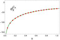
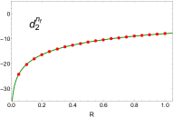
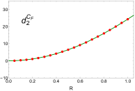
Figure 3: Two-loop collinear anomaly exponent of the $p_{T}$-veto soft function. The (red) dots represent our numbers and the solid (green) lines are the fit functions from [19, 20, 21].

We finally consider the standard jet-veto soft function that is based on transverse momenta. This is our first example of a SCET-2 observable with $n=0$, for which we compute the two-loop anomaly exponent $d_{2}$ that was defined in (11). The anomaly exponent has a similar colour decomposition,

$$d_{2} =d_{2}^{C_{A}}\;C_{F}C_{A}+d_{2}^{n_{f}}\;C_{F}T_{F}n_{f}+d_{2}^{C_{F}}\;C_{F}^{2}\,,$$ (14)

and the $p_{T}$-veto soft function again renormalises multiplicatively in cumulant space. At NLO one finds $d_{1}=0$ and at NNLO one obtains a similar picture as for the rapidity-dependent jet vetoes. Our results for $d_{2}$ are shown in Figure 3 together with fitting functions that were obtained in previous calculations [19, 20, 21]. Our results are once more in agreement with the existing results.

6 Conclusions

We have developed an algorithm that allows for an automated calculation of arbitrary two-loop soft functions that are defined in terms of two back-to-back light-like Wilson lines. The algorithm has been implemented in the custom program SoftSERVE, which can be used to determine both SCET-1 and SCET-2 soft functions. We illustrated the use of SoftSERVE with a few examples that are sensitive to jet clustering effects and hence violate the NAE theorem. Our results for the soft-drop jet-grooming soft function superseed previous determinations of the two-loop anomalous dimension that were valid only for specific values of the jet-grooming parameter. We plan to publish SoftSERVE in the near future.