Subpolynomial trace reconstruction for random strings and arbitrary deletion probability

Abstract

The insertion-deletion channel takes as input a bit string $\mathbf{x}\in\{0,1\}^{n}$, and outputs a string where bits have been deleted and inserted independently at random. The trace reconstruction problem is to recover $\mathbf{x}$ from many independent outputs (called “traces”) of the insertion-deletion channel applied to $\mathbf{x}$. We show that if $\mathbf{x}$ is chosen uniformly at random, then $\exp(O(\log^{1/3}n))$ traces suffice to reconstruct $\mathbf{x}$ with high probability. For the deletion channel with deletion probability $q<1/2$ the earlier upper bound was $\exp(O(\log^{1/2}n))$. The case of $q\geq 1/2$ or the case where insertions are allowed has not been previously analyzed, and therefore the earlier upper bound was as for worst-case strings, i.e., $\exp(O(n^{1/3}))$. We also show that our reconstruction algorithm runs in $n^{1+o(1)}$ time.

A key ingredient in our proof is a delicate two-step alignment procedure where we estimate the location in each trace corresponding to a given bit of $\mathbf{x}$. The alignment is done by viewing the strings as random walks and comparing the increments in the walk associated with the input string and the trace, respectively.

1 Introduction

Learning a parameter from a sequence of noisy observations is a basic problem in statistical inference and machine learning. The amount of data required (known as the sample complexity) to learn the parameter is of fundamental interest. A natural problem in this class where the missing parameter is a bit string and it is unknown whether the sample complexity is polynomial, is the trace reconstruction problem for the insertion-deletion channel. This channel takes as input a string $\mathbf{x}=(x_{0},x_{1},\dots,x_{n-1})\in\{0,1\}^{n}$ and outputs a noisy version of it, where bits have been randomly inserted and deleted. Let $q\in[0,1)$ be the deletion probability and let $q^{\prime}\in[0,1)$ be the insertion probability. First, for each $j$, before the $j$th bit of $\mathbf{x}$ we insert $G_{j}-1$ uniform and independent bits, where the independent geometric random variables $G_{j}\geq 1$ have parameter $1-q^{\prime}$. Then we delete each bit of the resulting string independently with probability $q$. The output string $\widetilde{\mathbf{x}}$ is called a trace. An example is shown in Figure 1.

Figure 1: We obtain a trace $\widetilde{\mathbf{x}}$ by sending $\mathbf{x}$ through the insertion-deletion channel. Inserted bits are shown in green and deleted bits are shown in red.

Suppose that the input string $\mathbf{x}$ is unknown. The trace reconstruction problem asks the following: How many i.i.d. copies of the trace $\widetilde{\mathbf{x}}$ do we need in order to determine $\mathbf{x}$ with high probability? (A more formal problem description will be given in Section 3.)

There are two variants of this problem: the “worst case” and the “average case” (also referred to as the “random case”). In the worst case variant, we want to obtain bounds which hold uniformly over all possible input strings $\mathbf{x}$. In the average case variant, the input string is chosen uniformly at random.

In this paper, we study the average case. Holenstein, Mitzenmacher, Panigrahy, and Wieder [HMPW08] gave an algorithm for reconstructing random strings from the deletion channel using polynomially many traces, assuming the deletion probability $q$ is sufficiently small. Peres and Zhai [PZ17] proved that $\exp(O(\log^{1/2}n))$ many traces suffice for the deletion channel when the deletion probability $q$ is below $1/2$. For $q\geq 1/2$, the previous best bound was the same as for worst case strings, i.e., $\exp(O(n^{1/3}))$, see [DOS17, NP17].

The following theorem is our main result, which improves the upper bound for all $q\in[0,1)$ and also holds when we allow insertions. In particular, we answer the part of the first open question in [Mit09, Section 9] which concerns random strings.

Theorem 1.

For $n\in\mathbbm{N}$ let $\mathbf{x}\in\{0,1\}^{n}$ be a bit string where the bits are chosen uniformly and independently at random. Given $q,q^{\prime}\in[0,1)$ there exists $M>0$ such that for all $n$ we can reconstruct $\mathbf{x}$ with probability $1-o_{n}(1)$ using $\lceil\exp(M\log^{1/3}n)\rceil$ traces from the insertion-deletion channel with parameters $q$ and $q^{\prime}$. Moreover, our algorithm runs in $n^{1+o(1)}$ time.

An earlier version of this work appeared in COLT [HPP18]; in this updated version, we have simplified the proof and added an analysis of the algorithm’s running time.

We remark that the trace reconstruction problem is significantly more difficult for $q>1/2$ and that the alignment algorithm used by Peres and Zhai fails fundamentally in this case. Moreover, the upper bound $\exp(O(\log^{1/3}n))$ in Theorem 1 is the best one can obtain without also improving the upper bound $\exp(O(n^{1/3}))$ for worst case strings. Indeed, given an arbitrary string of length $m=\log_{2+\varepsilon}n$ for $\varepsilon>0$, this string will appear in a random length $n$ string with probability converging to 1 as $n\rightarrow\infty$. In particular, a given worst case string of length $m$ is likely to appear in our random string, and the best known algorithm for reconstructing this string requires $\exp(\Omega(m^{1/3}))=\exp(\Omega(\log^{1/3}n))$ traces. See Lemma 10 in [MPV14] for the details of this reduction.

We note also that our methods can be adapted easily to certain other reconstruction problems, e.g., to the case where one allows substitutions in addition to deletions and insertions, and the case where the bits in the input $\mathbf{x}$ are independent Bernoulli($r$) random variables for arbitrary $r\in(0,1)$, instead of $r=1/2$. There is also a simple reduction (described in e.g. [MPV14] and [DOS17]) of the trace reconstruction problem for larger alphabets to the case of bits. Moreover, as shown in [MPV14], trace reconstruction becomes much easier if the alphabet size grows as $\Omega(\log n)$.

In Section 2 we present some background and literature on the trace reconstruction problem, before we give a precise definition of the trace reconstruction problem in Section 3. We give an outline of the proof of Theorem 1 in Section 4 and we present some notation in Section 5. In Sections 6 to 9 we prove the various ingredients which are needed for the proof of Theorem 1, and in Section 10 we conclude the proof.

2 Related work

The trace reconstruction problem dates back to the early 2000’s [Lev01a, Lev01b, BKKM04]. Batu, Kannan, Khanna, and McGregor, who were partially motivated by the study of genetic mutations, considered the case where the deletion probability $q$ is decreasing in $n$. They proved that if the original string $\mathbf{x}$ is random and the deletion probability $q=O(1/\log n)$, then $\mathbf{x}$ can be constructed with high probability using $O(\log n)$ samples. Furthermore, they proved that if $q=O(n^{-(1/2+\varepsilon)})$, then every string $\mathbf{x}$ can be reconstructed with high probability with $O(n\log n)$ samples.

Holenstein, Mitzenmacher, Panigrahy, and Wieder [HMPW08] considered the case of random strings and constant deletion probability. They gave an algorithm for reconstruction with polynomially many traces when the deletion probability $q$ is less than some small threshold $c$. The threshold $c$ is not given explicitly in the work of [HMPW08], but was estimated in [PZ17] to be at most $0.07$.

The result of [HMPW08] was improved by [PZ17]. They showed that a subpolynomial number of traces $\exp(O(\log^{1/2}n))$ is sufficient for reconstruction, and they extended the range of allowed $q$ to the interval $[0,1/2)$.

Our work improves the above results in three ways. First, we improve the upper bound to $\exp(O(\log^{1/3}n))$. Second, we allow for any deletion and insertion probabilities in $[0,1)$. Third, unlike [PZ17], our method works not only for the deletion channel, but also for the case where we allow insertions and substitutions.

It is shown by [HMPW08] that $\exp(O(n^{1/2}\log n))$ traces suffice for reconstruction with high probability with worst case input. This was improved to $\exp(O(n^{1/3}))$ independently by De, O’Donnell, and Servedio [DOS17] and by Nazarov and Peres [NP17]. Until the current work, the average case upper bound was equal to the worst case upper bound for $q\geq 1/2$. The techniques developed by [DOS17, NP17] are applied in the current work and the work of [PZ17] to certain shorter substrings of our random string.

A lower bound of $\Omega(\log^{2}n)$ was obtained in the average case in [MPV14], and a lower bound of $\Omega(n)$ was obtained in the worst case in [BKKM04]. These bounds were improved to $\Omega(\log^{9/4}n/\sqrt{\log\log n})$ and $\Omega(n^{5/4}/\sqrt{\log n})$, respectively, by Holden and Lyons [HL18], and further to $\Omega(\log^{5/2}n/(\log\log n)^{7})$ and $\Omega(n^{3/2}/\log^{7}n)$ by Chase [Cha19]. Trace reconstruction for the setting which allows insertions and substitution in addition to deletions was considered in [KM05, VS08, DOS17, NP17]. We refer to the introduction of [DOS17] and the survey [Mit09] for further background on the deletion channel.

3 The trace reconstruction problem

To simplify notation, throughout the paper we will implicitly pad any finite-length bit strings with infinitely many zeroes on the right. Thus, expressions such as $\mathbf{x}(i:j)$ are well-defined for $i<j$ even if $j$ is larger than the length of $\mathbf{x}$. Let $\mathbbm{N}=\{0,1,\dots\}$, and let $\mathcal{S}:=\{0,1\}^{\mathbbm{N}}$ denote the space of infinite sequences of zeroes and ones. We denote elements of $\mathcal{S}$ by $\mathbf{x}:=(x_{0},x_{1},\ldots)$. If $I\subset\mathbbm{R}$ we will sometimes write $\mathbf{x}(I)$ instead of $\mathbf{x}(I\cap\mathbbm{N})$, and we use a similar convention for functions which are defined on (subsets of) $\mathbbm{N}$.

Fix a deletion probability $q$ and an insertion probability $q^{\prime}$ in $[0,1)$, and let $p=1-q$ and $p^{\prime}=1-q^{\prime}$. We construct $\widetilde{\mathbf{x}}$ from $\mathbf{x}$ by the procedure described above, i.e., first, for each $j\in\mathbbm{N}$ we insert $G_{j}-1$ uniform and independent bits before the $j$th bit of $\mathbf{x}$. The geometric random variables $G_{j}$ are independent and satisfy

$$\mathbbm{P}[G_{j}=v]=(q^{\prime})^{v-1}(1-q^{\prime}),\qquad\forall v\in\{1,2,\dots\}.$$

Then we delete each bit of the resulting string independently with probability $q$.

Let $\mu$ be the law of i.i.d. Bernoulli random variables with parameter $1/2$. We write $\mathbbm{P}_{\mathbf{x}}:=\mathbbm{P}_{\delta_{\mathbf{x}}}$ for the law of $\widetilde{\mathbf{x}}$ when $\mathbf{x}$ is fixed and write $\mathbbm{P}:=\mathbbm{P}_{\mu}$ for the law of $\widetilde{\mathbf{x}}$ when $\mathbf{x}$ is picked according to $\mu$. We call the string $\widetilde{\mathbf{x}}$ a trace. An example is given in Figure 1.

Worst case reconstruction problem

Let $q,q^{\prime}\in[0,1)$. For any $N\in\mathbbm{N}$ let $\mathbbm{P}_{\mathbf{x}}^{N}$ denote the probability measure associated with $N$ independent outputs of the insertion-deletion channel $\mathbbm{P}_{\mathbf{x}}$ with deletion (resp. insertion) probability $q$ (resp. $q^{\prime}$). For $n\in\mathbbm{N}$ and $\mathbf{x}\in\{0,1\}^{n}$ let $\mathfrak{X}$ denote a collection of $N_{n}\in\mathbbm{N}$ traces sampled independently at random. We say that worst case strings of length $n$ can be reconstructed with probability $1-o_{n}(1)$ from $N_{n}$ traces, if there is a function $G\colon\mathcal{S}^{N_{n}}\to\{0,1\}^{n}$, such that for all $\mathbf{x}\in\mathcal{S}$,

$$\mathbbm{P}_{\mathbf{x}}^{N_{n}}[G(\mathfrak{X})=\mathbf{x}(0:n-1)]=1-o_{n}(1).$$

Average case reconstruction problem

Let $\mu_{n}$ denote uniform measure on $\{0,1\}^{n}$. We say that uniformly random strings of length $n$ can be reconstructed with probability $1-o_{n}(1)$ from $N_{n}$ traces if we can find a set $\mathcal{S}_{n}\subset\{0,1\}^{n}$ with $\mu_{n}(\mathcal{S}_{n})=1-o_{n}(1)$, and a function $G\colon\mathcal{S}^{N_{n}}\to\{0,1\}^{n}$, such that for all $\mathbf{x}\in\mathcal{S}$ for which $\mathbf{x}(0:n-1)\in\mathcal{S}_{n}$, we have

$$\mathbbm{P}_{\mathbf{x}}^{N_{n}}[G(\mathfrak{X})=\mathbf{x}(0:n-1)]=1-o_{n}(1).$$

In particular, Theorem 1 says that uniformly random strings can be reconstructed from $N_{n}:=\lceil\exp(M\log^{1/3}n)\rceil$ traces with probability $1-o_{n}(1)$.

4 Outline of proof

We give here an informal description of the algorithm used to achieve the bound in Theorem 1. The bits of $\mathbf{x}$ will be recovered one by one: for any $k,n\in\mathbbm{N}$ with $k<n$ we assume $\mathbf{x}(0:k)$ is already known, and we show that with probability $1-O(n^{-2})$ we can use $\lceil\exp(M\log^{1/3}n)\rceil$ traces to determine the subsequent bit $x_{k+1}$. We will reuse these same traces for each step (i.e., for all values of $k$). Even with this reuse, by a union bound, the reconstruction will succeed at every step with high probability.

Three ingredients are required, as follows:

1. A Boolean test $T(\mathbf{w},\widetilde{\mathbf{w}})$ on pairs $(\mathbf{w},\widetilde{\mathbf{w}})$ of bit strings indicating whether $\widetilde{\mathbf{w}}$ is a plausible match for the string $\mathbf{w}$ sent through the insertion-deletion channel.

2. An alignment procedure that uses the test $T$ repeatedly to produce for each of the independent traces $\widetilde{\mathbf{x}}$ an estimate $\tau$ for the position in $\widetilde{\mathbf{x}}$ corresponding to the $k$-th bit of $\mathbf{x}$.

3. A bit recovery procedure based on a method of [PZ17, DOS17, NP17] to produce from the approximately aligned traces an estimate of the subsequent bit or bits.

The argument of [PZ17] follows the same overall structure, with an alignment step followed by a reconstruction step for each bit in the original string. However, the greedy alignment step of [PZ17] relies crucially on the assumption that the deletion probability $q<1/2$, and that no insertions are allowed. We overcome this problem by introducing a new kind of test for the alignment based on studying correlations between blocks in the input string and in the trace.

4.1 The test $T$

We describe here a simplified version of the test $T(\mathbf{w},\widetilde{\mathbf{w}})$, which returns $1$ if there is a likely match and $0$ otherwise. Assume for simplicity that $\mathbf{w}$ and $\widetilde{\mathbf{w}}$ have the same length and that $q=q^{\prime}$, so the expected output length of the insertion-deletion channel is the same as the input length. The test involves two parameters: the length $\ell$ of the strings to test and another parameter $\lambda\leq\sqrt{\ell}$. We subdivide both $\mathbf{w}$ and $\widetilde{\mathbf{w}}$ into roughly $\ell/\lambda$ blocks of size $\lambda$. We use $T_{\ell,\lambda}$ to denote the test using these parameters.

For each $i$, let $s_{i}$ be the number of $1$’s minus the number of $0$’s in the $i$-th block of $\mathbf{w}$, and similarly define $\widetilde{s}_{i}$ for $\widetilde{\mathbf{w}}$. For some fixed constant $c>0$ to be specified later, we declare that

$$T_{\ell,\lambda}(\mathbf{w},\widetilde{\mathbf{w}})=\begin{cases}1&\text{if }\displaystyle\sum_{i=1}^{\left\lceil\ell/\lambda\right\rceil}\operatorname{sign}(s_{i})\cdot\operatorname{sign}(\widetilde{s}_{i})>c\cdot\frac{\ell}{\lambda},\\ 0&\text{otherwise}.\end{cases}$$

See Figure 2 for an illustration. The idea here is that if the bits in the $i$th block of $\widetilde{\mathbf{w}}$ did not come from the $i$th block of $\mathbf{w}$, then they will be independent random bits, and so each $\operatorname{sign}(s_{i})\cdot\operatorname{sign}(\widetilde{s}_{i})$ will be $1$ or $-1$ with equal probability (if we ignore the small probability event on which $s_{i}$ or $\widetilde{s}_{i}$ is equal to 0, in which case we have $\operatorname{sign}(s_{i})\cdot\operatorname{sign}(\widetilde{s}_{i})=0$). In this case, by Hoeffding’s inequality, the test declares a match with probability $e^{-\Omega(\ell/\lambda)}$. Let us call this situation a “spurious match”.

Figure 2: Illustration of the test $T_{\ell,\lambda}(\mathbf{w},\widetilde{\mathbf{w}})$ with $\ell=15$ and $\lambda=3$. The arrows indicate that a bit in $\mathbf{w}$ was copied to a bit in $\widetilde{\mathbf{w}}$.

On the other hand, if one of the bits in the $i$-th block of $\widetilde{\mathbf{w}}$ was copied over from somewhere in the $i$-th block of $\mathbf{w}$ for some $i$, we consider the match to be a “true match”. Let us describe one relatively likely way in which this could happen. Suppose that a positive fraction of the bits in the $i$-th block of $\widetilde{\mathbf{w}}$ came from the $i$-th block of $\mathbf{w}$. There is roughly a $e^{-O(\ell/\lambda^{2})}$ chance that this will happen for all $i$ (comparable to the probability that a simple random walk stays within $[-\lambda,\lambda]$ for $\ell$ steps). In this case, it is quite likely for a match to occur, because each $\operatorname{sign}(s_{i})$ and $\operatorname{sign}(\widetilde{s}_{i})$ will be positively correlated.

To summarize, the main feature of our test is that it has a true match rate of at least $e^{-O(\ell/\lambda^{2})}$ and a spurious match rate of at most $e^{-\Omega(\ell/\lambda)}$, which is much lower than the true match rate as long as $\lambda$ is large enough. In order to make these statements rigorous, however, the real test we use (as well as the precise notions of “true” or “spurious” match) is slightly more complicated than what is described above. The test is defined formally in Section 6.

4.2 Alignment

We first remark that our alignment procedure will actually fail for most (all but about $e^{-O(\log^{1/3}n)}$) of the traces, and we will disregard these failed traces for purposes of reconstructing the current bit. Nevertheless, by taking enough total traces (more precisely, by choosing the constant $M$ in Theorem 1 sufficiently large), we will still have a sufficient number of successful alignments to work with.

The alignment $\tau$ is computed in two steps. See Figure 3. We first compute a preliminary alignment position $\tau_{1}$ in the output which corresponds to position $k_{1}:=k-C\log n$ in the input (where $C$ is some large enough constant). This is done by performing the test $T_{\ell,\lambda}$ with $(\ell,\lambda)=(C\log^{5/3}n,C^{1/2}\log^{2/3}n)$. In particular, we declare $\tau_{1}$ to be the first index in the output for which

$$T_{\ell,\lambda}(\mathbf{x}(k_{1}-\ell+1:k_{1}),\widetilde{\mathbf{x}}(\tau_{1}-\ell+1:\tau_{1}))=1.$$

Assuming that such a $\tau_{1}$ exists, we claim that $\tau_{1}$ is very likely to have alignment error of order at most $O(C\log n)$.

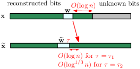
Figure 3: Illustration of the two alignment steps. In each step we fix a substring $\mathbf{w}$ of $\mathbf{x}$ which has distance $O(\log n)$ from the first unknown bit. Assuming the test gives a positive result with some substring $\widetilde{\mathbf{w}}$ of the trace, the alignment error (indicated by the lower horizontal arrow) is the difference between the right end-point $\tau$ of $\widetilde{\mathbf{w}}$ and the position in $\widetilde{\mathbf{x}}$ corresponding to the right end-point of $\mathbf{w}$ (indicated by the vertical red arrow).

The probability of a spurious match is $e^{-\Omega(\ell/\lambda)}=e^{-\Omega(C^{1/2}\log n)}=n^{-\Omega(C^{1/2})}$, which is negligible for large enough $C$. This probability is so small that even taking a union bound over all substrings of length $\ell$, we are unlikely to find a single length-$\ell$ substring that produces spurious matches at a high rate.

Meanwhile, the probability of a true match is at least $e^{-O(\ell/\lambda^{2})}\geq e^{-O(\log^{1/3}n)}$. A true match in this case means that for some $i$ with $1\leq i\leq\ell$, the bit in position $k_{1}-\ell+i$ of the input was copied to somewhere very close to position $\tau_{1}-\ell_{i}$ in the output (as will be made precise later).

However, this does not guarantee that the alignment error of $\tau_{1}$ is $O(C\log n)$: it could happen that between positions $k_{1}-\ell+i$ and $k_{1}$, the difference between the number of insertions and deletions is more than $C\log n$. See Figure 4 for an illustration of this effect. By Hoeffding’s inequality, the probability this happens is at most $e^{-\Omega\left((C\log n)^{2}/\ell\right)}=e^{-\Omega(C\log^{1/3}n)}$, so that with $C$ large enough, this misalignment scenario happens rarely compared to the true match probability described above.

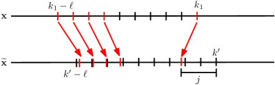
Figure 4: The red arrows indicate to what position a few bits (represented by the vertical red line segments) in the input string are copied in the trace. The vertical line segments (black or red at the top; black at the bottom) indicate the blocks of length $\lambda$ which are used by the test $T_{\ell,\lambda}$. In the example we may get a positive test with the intervals $\mathbf{x}(k_{1}-\ell+1:k_{1})$ and $\widetilde{\mathbf{x}}(k^{\prime}-\ell+1:k^{\prime})$ although the alignment error $j$ is rather large, since the number of deletions minus the number of insertions in the latter part of the trace happens to be particularly large, which gives a good overlap between the blocks at the beginning of the string but not at the end.

4.3 Fine alignment and bit statistics

Once we have aligned to within $O(\log n)$, we will perform a second alignment step to align within roughly $O(\log^{1/3}n)$. This involves performing the test $T_{\ell,\lambda}$ with $(\ell,\lambda)=(C^{2/3}\log^{1/3}n,C^{1/12})$. This gives a true match rate of $e^{-O(\ell/\lambda^{2})}=e^{-O(C^{1/2}\log^{1/3}n)}$ and spurious match rate of $e^{-\Omega(\ell/\lambda)}=e^{-\Omega(C^{7/12}\log^{1/3}n)}$, so the true matches dominate the spurious ones.

However, the chance of spurious matches is not low enough to union bound over all substrings of length $\ell=C^{2/3}\log^{1/3}n$ that we might align to. In fact, it is actually quite likely that there will be some “bad” substring of length $\ell$ in the input that produces a high rate of spurious matches (for example, imagine having two nearby runs of $\ell$ consecutive $0$’s in the input). Getting around this problem requires some care; the main idea is that although there may be some bad length-$\ell$ substrings, it is very unlikely that every single length-$\ell$ substring in an interval of size $\log n$ is bad, and we use one of the not bad strings to align.

The end result of our two alignment steps is some position $\tau_{2}$ in the output which has an alignment error of $O(\log^{1/3}n)$ to some specified location $k_{*}$ in the input string $\mathbf{x}$ (i.e., the input position corresponding to $\tau_{2}$ is within $O(\log^{1/3}n)$ of $k_{*}$). Furthermore, $k_{*}$ is within the last $O(\log n)$ positions of what we have reconstructed so far (i.e., $k-k_{*}=O(\log n)$).

We can then use a variant of the worst case reconstruction algorithm from [DOS17, NP17] (which was also used in [PZ17]) to reconstruct $\mathbf{x}(k_{*}:k_{*}+C\log n)$ using $e^{O(\log^{1/3}n)}$ (approximate) traces $\widetilde{\mathbf{x}}(\tau_{2}:\infty)$, where shifting of $O(\log^{1/3}n)$ can be tolerated. The algorithm is based on looking at individual bit statistics, and the key property can be roughly stated as follows: consider two possibilities for the string $\mathbf{x}$ which match the first $k$ bits reconstructed so far but disagree on the $(k+1)$-th bit. Then, there will be a noticeable ($e^{-O(\log^{1/3}n)}$) difference in the expected value of one of the positions in $\widetilde{\mathbf{x}}(\tau_{2}:\infty)$, which allows us to statistically distinguish the two possibilities. A precise formulation is given in Lemma 20.

4.4 Implementing the algorithm efficiently

While we have thus far given a complete description of how to do trace reconstruction using $e^{O(\log^{1/3}n)}$ traces, there are several obstacles to making this algorithm run in $n^{1+o(1)}$ time.

First, during the alignment stage as described so far, we perform our test $T$ on a sliding window that potentially passes over the whole output string. This is at least $O(n)$ work needed for reconstructing even a single bit, which would lead to an overall running time no better than $O(n^{2})$. However, it is quite wasteful to compute our alignment from scratch each time we reconstruct a new bit. Instead, we can use previous alignments as a rough guide, allowing us to skip past all but $n^{o(1)}$ bits of the output string.

Next, to determine the good index $k_{2}$, we need some way of assessing whether a given string of length $\log^{1/3}n$ behaves well with our test $T$ in terms of having a high true match rate and low spurious match rate. While explicitly calculating these probabilities is not straightforward, we can estimate them by Monte-Carlo simulation. Recall that the probabilities in question are of order $e^{-O(\log^{1/3}n)}=n^{-o(1)}$, so only $n^{o(1)}$ samples are required to achieve a good enough accuracy.

Finally, in the actual reconstruction step (based on bit statistics as described in the last paragraph of Section 4.3), a naive implementation requires us to test every possibility for the first roughly $\log n$ unreconstructed bits. However, as observed in [HMPW08], the comparison of bit statistics may be formulated as a linear program, which can be solved much more efficiently.

5 Notation for the insertion-deletion channel and Markov properties

Let us introduce some general notation and conventions that will be used for the rest of the paper. To lighten notation, we fix once and for all two values $q,q^{\prime}\in[0,1)$ for the deletion and insertion probability, respectively. In order to simplify notation, we will further assume throughout that

$$q=q^{\prime},$$ (1)

so that the expected length of the output equals the length of the input. The same arguments carry through in a straightforward way for general $q,q^{\prime}$ with appropriate scaling of output lengths. We will use big-$O$ notation, and all implicit constants in $O(\,\cdot\,)$ and $\Omega(\,\cdot\,)$ expressions may depend on $q$ and $q^{\prime}$ but nothing else.

We will also need to control the relative sizes of various constant factors. To this end, we introduce a parameter $C$ which will appear in some of our bounds, which should be thought of as a “large constant”. We will ultimately complete our argument by choosing $C$ to be sufficiently large (where the threshold for being large enough depends only on $q$ and $q^{\prime}$).

Next, let us introduce some notation relating to strings and their traces. Recall that $\mathcal{S}:=\{0,1\}^{\mathbbm{N}}$ denotes the space of infinite sequences of zeroes and ones. Let $\Omega=\mathcal{S}\times[0,1]^{\mathbbm{N}}$. We denote the first coordinate function on $\Omega$ by $\mathbf{x}:=(x_{0},x_{1},\ldots)$ and the second by $\omega:=(\omega_{0},\omega_{1},\ldots)$. Let $U$ be the product uniform measure on $[0,1]^{\mathbbm{N}}$. If $\rho$ is any measure on $\{0,1\}^{\mathbbm{N}}$, let $\mathbbm{P}_{\rho}:=\rho\times U$. Thus, our previous notation can be expressed as $\mathbbm{P}_{\mathbf{x}}:=\mathbbm{P}_{\delta_{\mathbf{x}}}$ and $\mathbbm{P}:=\mathbbm{P}_{\mu}$, where $\mu$ is the law of i.i.d. Bernoulli random variables with parameter $1/2$.

We can construct the output $\widetilde{\mathbf{x}}=(\widetilde{x}_{0},\widetilde{x}_{1},\dots)$ of the insertion-deletion channel as a function of $\mathbf{x}$ and $\omega$, where $\omega$ represents the (random) pattern of insertions and deletions. The construction proceeds as follows. Temporarily denote $a:=q(1-q^{\prime})/(1-qq^{\prime})$ and $b:=q^{\prime}(1-q)/(1-qq^{\prime})$. For each $m\in\mathbbm{N}$ we define quantities $s(m),s^{\prime}(m)\in\mathbbm{N}$, where $s(m)$ (resp. $s^{\prime}(m)$) represents a position in $\mathbf{x}$ (resp. $\widetilde{\mathbf{x}}$) associated with the randomness of $\omega(m)$. We make the definition by setting $s(0)=s^{\prime}(0)=0$ and proceeding inductively for $m\geq 0$:

• If $\omega(m)\in[0,a]$, then define $s(m+1)=s(m)+1$ and $s^{\prime}(m+1)=s^{\prime}(m)$ (deletion).

• If $\omega(m)\in(a,a+b/2]$, then set $s(m+1)=s(m)$, $s^{\prime}(m+1)=s^{\prime}(m)+1$, and $\widetilde{x}_{s^{\prime}(m)}=0$ (insertion of 0).

• If $\omega(m)\in(a+b/2,a+b]$, then set $s(m+1)=s(m)$, $s^{\prime}(m+1)=s^{\prime}(m)+1$, and $\widetilde{x}_{s^{\prime}(m)}=1$ (insertion of 1).

• If $\omega(m)\in(a+b,1]$, then set $s(m+1)=s(m)+1$, $s^{\prime}(m+1)=s^{\prime}(m)+1$, and $\widetilde{x}_{s^{\prime}(m)}=x_{s(m)}$ (copy).

We will now justify briefly why this definition of the deletion-insertion channel is equivalent to the one given in Section 3. The channel described in Section 3 is equivalent to the following: (i) before bit $x_{j}$ insert $G_{j}$ uniform and independent bits, where $G_{j}$ is as before, (ii) delete each of the inserted bits independently with probability $q$, and (iii) delete each of the original bits independently with probability $q$. The combined effect of (i) and (ii) is to insert $\widehat{G}_{j}$ uniform and independent bits before bit $x_{j}$, where $\widehat{G}_{j}$ is a geometric random variable with parameter $b$. From this we conclude equivalence with the channel as described in the bullet points above, because in this channel we insert a geometric number of bits with parameter $b$ between each copy or deletion, and since the fraction of bits in the input string which are deleted is given by $b/(1-a-b)=q$.

Let us now introduce some notation for corresponding positions in input strings with positions in their traces. Define

$$\psi(j):=\inf\{t\geq 0\,:\,s(t)=j\},\qquad\widetilde{\psi}(j):=\sup\{t\geq 0\,:\,s^{\prime}(t)=j\}.$$

In other words, $\psi(j)$ is the index of the first coordinate in $\omega$ that decides whether to insert a bit before $x_{j}$. Similarly, $\widetilde{\psi}(j)$ is the index in $\omega$ that determines the value of $\widetilde{x}_{j}$. Next, define

$$f(k)=s^{\prime}(\psi(j)),\qquad g(k^{\prime})=s(\widetilde{\psi}(k^{\prime})).$$

In other words, $f(k)$ is the value of $s^{\prime}(m)$ at the first time when $s(m)=k$, and $g(k^{\prime})$ is the value of $s(m)$ at the first time when $s^{\prime}(m)=k^{\prime}$. See Figure 5 for an illustration. Roughly speaking, position $k$ in the input gets mapped to position $f(k)$ in the output, and position $k^{\prime}$ in the output was mapped to from position $g(k^{\prime})$ in the input. In particular, $g$ is an approximate inverse of $f$. We also define the function

$$d(k,k^{\prime})=\max\left(|f(k)-k^{\prime}|,|g(k^{\prime})-k|\right),$$ (2)

which measures the failure of position $k$ in the input to correspond to position $k^{\prime}$ in the output.

Figure 5: Illustration of the functions $f$ and $g$. The arrows indicate bits which are copied from $\mathbf{x}$ to $\widetilde{\mathbf{x}}$.

The next proposition records the Markov property that is satisfied by our insertion-deletion process. It will be convenient to use the notation $\theta$ to denote the shift operator on bit strings, i.e., $\theta(\mathbf{x})=\mathbf{x}(1:\infty)$ and more generally, $\theta^{k}(\mathbf{x})=\mathbf{x}(k:\infty)$.

Proposition 2.

For any $m\geq 0$, conditioned on the values of $s(m)$ and $s^{\prime}(m)$, the string $\theta^{s^{\prime}(m)}(\widetilde{\mathbf{x}})$ has the same law as a trace from $\theta^{s(m)}(\mathbf{x})$ through the insertion-deletion channel. In particular, for any $t\geq 0$, the law of $\theta^{t}(\widetilde{\mathbf{x}})$ is $\mathbbm{P}_{\theta^{g(t)}(\mathbf{x})}$.

Proof.

This is almost immediate from the way we contructed the insertion-deletion channel in terms of $\omega$. It is clear that the increments of $(s(m),s^{\prime}(m))$ are i.i.d. Thus, starting $(s(m),s^{\prime}(m))$ from a specified value simply amounts to ignoring the first $s(m)$ bits of the input and writing to the output starting from position $s^{\prime}(m)$. ∎

6 Clear robust bias test

We now give a formal definition of the test $T_{\ell,\lambda}$. Recall that the test is designed to answer whether a substring $\widetilde{\mathbf{w}}$ of length $\ell$ in a trace is likely to have come from a substring $\mathbf{w}$ of the same length in the already recovered part of the input. The test involves subdivision into “blocks” of size approximately $\lambda\leq\sqrt{\ell}$. We remark that the test will be applied for $(\ell,\lambda)$ on two different scales, namely of order $(\log^{5/3}n,\log^{2/3}n)$ and $(\log^{1/3}n,1)$.

Given a string $\mathbf{w}:=\mathbf{x}(k-\ell+1:k)$, let $d:=\left\lceil\ell/\lambda\right\rceil$ denote the number of blocks. The right endpoints of the blocks $\{u_{i}\}$ will be given by $u_{i}:=k-\ell+\lceil i\ell/d\rceil$. Because $\lambda\leq\sqrt{\ell}\leq d$, this definition makes $\{(u_{i-1},u_{i}]:1\leq i\leq d\}$ a partition of $(k-\ell,k]$ into consecutive intervals of length $\lambda$ or $\lambda-1$.

Let us define the robust bias of a block $\mathbf{x}(u_{i-1}+1:u_{i})$ to be

$$\lambda^{-1/2}\inf_{\begin{subarray}{c}\text{$t_{1},t_{2}\in\mathbbm{N}\,:\,$}\\ \text{$|t_{1}-u_{i-1}|<\lambda/100$}\\ \text{$|t_{2}-u_{i}|<\lambda/100$}\\ \end{subarray}}\Big{|}\sum_{j=t_{1}}^{t_{2}}(2x_{j}-1)\Big{|}.$$ (3)

We say that a block has a clear robust bias if its robust bias is at least 1. See Figure 6 for an illustration.

Figure 6: The length of the vertical arrow describes the robust bias associated with the block $\mathbf{x}(u_{i-1}+1:u_{i})$. The curve represents the partial sums $\lambda^{-1/2}\sum_{j}(2x_{j}-1)$, renormalized to equal 0 at $u_{i-1}$. We say that the robust bias is clear if it is at least 1, such as shown in the given example.

For some $\theta\in(0,1/10)$ let $\mathcal{I}\subset\{1,\dots,d\}$ be the indices of the $\lceil\theta d\rceil$ blocks for which the robust bias is largest (with ties resolved in some arbitrary way). By Donsker’s theorem, for $\theta$ sufficiently small and $\lambda$ sufficiently large compared to $\theta$, it holds with high probability for large $\ell$ that all blocks in $\mathcal{I}$ have a clear robust bias. We fix such a choice of $\theta$ as follows: for $B$ a standard Brownian motion, let

$$\theta:=\frac{1}{10}\mathbbm{P}\left[\inf_{t_{1}\in[0,1/50],t_{2}\in[1,1+1/50]}|B_{t_{2}}-B_{t_{1}}|>1\right]>0\,.$$ (4)

For each $i$, define the quantity

$$s_{i}:=\sum_{j=u_{i-1}+1}^{u_{i}}(2x_{j}-1)$$ (5)

which counts the number of 1’s minus the number of 0’s in the $i$-th block. Define $\widetilde{s}_{i}$ similarly for a string $\widetilde{\mathbf{w}}$ of the same length as $\mathbf{w}$. We first define our test using an extra parameter $c\in(0,1)$. The test is given by

$$T^{c}_{\ell,\lambda}(\mathbf{w},\widetilde{\mathbf{w}})=\begin{cases}1&\text{if }\displaystyle\sum_{i\in\mathcal{I}}\operatorname{sign}(s_{i})\cdot\operatorname{sign}(\widetilde{s}_{i})>c|\mathcal{I}|,\\ 0&\text{otherwise},\end{cases}$$

where $|\mathcal{I}|$ denotes the cardinality of $\mathcal{I}$. We will only apply the test for a particular value of $c$, which will be chosen depending on the insertion/deletion probabilities as described in the next subsection.

6.1 Estimates for the test $T$

Definition 3.

We say that a string $\widetilde{\mathbf{w}}$ of length $\ell$ has clear robust bias at scale $\lambda$ if at least $\lceil\theta d\rceil=|\mathcal{I}|$ of its blocks have clear robust bias.

First, we formally state our earlier claim that due to our sufficiently small choice of $\theta$, a random string has clear robust bias with high probability.

Lemma 4.

Let $\mathbf{w}$ be a random string of length $\ell$. Then, $\mathbf{w}$ fails to have clear robust bias at scale $\lambda$ with probability at most $e^{-\Omega(\ell/\lambda)}$.

Proof.

Within a single block, by Donsker’s theorem, the partial sums of the bits converge to Brownian motion as $\lambda\rightarrow\infty$. Thus, for sufficiently large $\lambda$, the probability that this block has clear robust bias is at least $2\theta$. Consequently, the probability that the proportion of blocks with clear robust bias is less than $\theta$ is exponentially small in the number of blocks, i.e., it is of order $e^{-\Omega(\ell/\lambda)}$. ∎

Lemma 5.

Let $\mathbf{w}$ be a string of length $\ell$ which exhibits robust bias at scale $\lambda$. Suppose that we take a trace $\widetilde{\mathbf{w}}$ of $\mathbf{w}$ through the insertion-deletion channel. Then, for a small enough constant $c>0$ depending only on the insertion/deletion probabilities, we have

$$\mathbbm{P}\left(T^{c}_{\ell,\lambda}(\mathbf{w},\widetilde{\mathbf{w}}(0:\ell-1))=1\right)\geq e^{-O(\ell/\lambda^{2})}.$$

In order to prove Lemma 5, we first define a condition describing when $\mathbf{w}$ and $\widetilde{\mathbf{w}}$ are unusually well aligned. We will then show that $T^{c}_{\ell,\lambda}$ is reasonably likely to test positive conditioned on this good alignment.

Definition 6.

Let $\mathbf{w}$ be a string of length $\ell$ and $\widetilde{\mathbf{w}}$ a trace of $\mathbf{w}$ through the insertion-deletion channel. Following the notation of this section, for a block size $\lambda$, we let $d=\lceil\ell/\lambda\rceil$, and we let $\{u_{i}\}_{i=0}^{d}$ denote the endpoints of the blocks. We say that the trace is $s$-aligned if for each $0\leq i\leq d$, it holds that

$$\left|(u_{i}-u_{0})-(f(u_{i})-f(u_{0}))\right|<s.$$

If the trace is $s$-aligned, we say that we have $s$-alignment.

Proof of Lemma 5.

Let $c_{0}$ be a small constant to be specified later. We first show that the probability of $c_{0}\lambda$-alignment is at least $e^{-O(\ell/c_{0}\lambda^{2})}$. For convenience, define the function

$$\zeta(x):=(x-u_{0})-(f(x)-f(u_{0})).$$

Consider any $\lambda$ consecutive blocks numbered $i+1$ through $i+\lambda$. Note that the sequence $\left\{\frac{\zeta(k)}{\lambda}\right\}_{k=u_{i}}^{u_{i+\lambda}}$ is a mean-zero simple random walk (since we assume $q=q^{\prime}$), where the distribution of the increments is determined by the insertion and deletion probabilities and has finite variance.

By Donsker’s theorem, $\left\{\frac{\zeta(k)}{\lambda}\right\}_{k=u_{i}}^{u_{i+\lambda}}$ converges to a constant multiple of standard Brownian motion as $\lambda\rightarrow\infty$ (where time is scaled by $\lambda^{2}$). For a standard Brownian motion $\{W_{t}\}_{0\leq t\leq 1}$, we have that

$$\mathbbm{P}\Big{(}W_{0},W_{1}\in[-c_{0}/2,c_{0}/2]\text{ and $|W_{t}|\leq c_{0}$ for all $0\leq t\leq 1$}\Big{)}=e^{-O(1/c_{0})},$$

Thus, we have a similar statement for the quantities $\frac{\zeta(k)}{\lambda}$, where

$$\mathbbm{P}\left(\frac{|\zeta(u_{i})|}{\lambda}\leq\frac{c_{0}}{2},\;\;\frac{|\zeta(u_{i+\lambda})|}{\lambda}\leq\frac{c_{0}}{2},\;\;\text{and}\;\;{\displaystyle\max_{i<j<i+\lambda}\frac{|\zeta(u_{i+\lambda})|}{\lambda}\leq c_{0}}\right)\geq e^{-O(1/c_{0})}.$$

Chaining together these events for each group of $\lambda$ consecutive blocks (of which there are roughly $\ell/\lambda^{2}$), we see that the overall probability of being $c_{0}\lambda$-aligned is at least $e^{-O(\ell/c_{0}\lambda^{2})}$.

Our next step is to estimate the probability of a positive test conditioned on the trace being $c_{0}\lambda$-aligned. We further condition on the specific values of the $f(u_{i})$. Note that the substring $\mathbf{w}(u_{i}+1:u_{i+1})$ must be transformed into the substring $\widetilde{\mathbf{w}}(f(u_{i})+1:f(u_{i+1}))$. The insertion/deletion patterns of these transformations are all independent, and they have the same distribution as the insertion-deletion channel applied to $\mathbf{w}(u_{i}:u_{i+1}-1)$ conditioned on the output trace having length $f(u_{i+1})-f(u_{i})$.

Let $m_{i}$ denote the number of bits copied to $\widetilde{\mathbf{w}}(f(u_{i}):f(u_{i+1})-1)$ from $\mathbf{w}(u_{i}:u_{i+1}-1)$, and note that we have $m_{i}=\Omega(\lambda)$ with probability $1-e^{-\Omega(\lambda)}$. Also, since we assume that our trace is $c_{0}\lambda$-aligned, only $O(c_{0}\lambda)$ bits in $\widetilde{\mathbf{w}}(u_{i}:u_{i+1}-1)$ were copied from outside of $\mathbf{w}(u_{i}:u_{i+1}-1)$. Finally, note that any bits in $\widetilde{\mathbf{w}}(u_{i}:u_{i+1}-1)$ which were not copied from $\mathbf{w}$ are i.i.d. uniformly random.

Recall that $\widetilde{\mathbf{w}}$ was assumed to have robust bias at scale $\lambda$. Thus, if $i\in\mathcal{I}$, then with probability $1-e^{-\Omega(\lambda)}$ we will have $\Omega(\sqrt{\lambda})$ bias in the sum of bits in $\widetilde{\mathbf{w}}(u_{i-1}:u_{i})$ copied from $\mathbf{w}$. It follows that for large enough $\lambda$ and small enough $c_{0}$, the correlation between $\operatorname{sign}(\widetilde{s}_{i})$ and $\operatorname{sign}(s_{i})$ is $\Omega(1)$. This means that (after all our conditioning) as long as $c$ is small enough, the test $T^{c}_{\ell,\lambda}$ will succeed except on an event with probability $e^{-\Omega(\ell/\lambda)}$.

In summary, there is at least a $e^{-O(\ell/\lambda^{2})}$ chance to have $\lambda$-alignment, and conditioning on this, a positive match occurs with high probability. This proves the lemma. ∎

From now on, we will always run our tests using the value of $c$ as in Lemma 5. Thus, we will henceforth simply write $T_{\ell,\lambda}$ instead of $T^{c}_{\ell,\lambda}$.

Definition 7.

Let $\mathbf{w}=\mathbf{x}(a+1:a+\ell)$ be a substring of the input, and let $\widetilde{\mathbf{w}}=\widetilde{\mathbf{x}}(b+1:b+\ell)$ be a substring of the same length taken from the trace. We say that $\mathbf{w}$ and $\widetilde{\mathbf{w}}$ are $s$-mismatched if for any $0\leq i\leq\ell$ it holds that $d(a+i,b+i)>s$, where $d$ is defined in (2).

Lemma 8.

Let $\mathbf{x}$ be a random string, and suppose we sample a trace $\widetilde{\mathbf{x}}$ from the insertion-deletion channel.

Consider two length-$\ell$ substrings $\mathbf{w}=\mathbf{x}(a+1:a+\ell)$ and $\widetilde{\mathbf{w}}=\widetilde{\mathbf{x}}(b+1:b+\ell)$. Let $\omega^{0}$ be a realization of the randomness of the insertion-deletion channel (i.e., an insertion/deletion pattern) for which $\mathbf{w}$ and $\widetilde{\mathbf{w}}$ are $\lambda$-mismatched. Then,

$$\mathbbm{P}\Big{(}T_{\ell,\lambda}(\mathbf{w},\widetilde{\mathbf{w}})=1\,\Big{|}\,\omega=\omega^{0}\Big{)}\leq e^{-\Omega(\ell/\lambda)}.$$

Proof.

Note that after conditioning on $\omega$, the remaining randomness is to sample the values of the bits. We do this incrementally block by block (where the blocks are of size $\lambda$). Suppose that we have already sampled the first $i-1$ blocks of $\mathbf{w}$ and $\widetilde{\mathbf{w}}$; let us consider the conditional distribution on bits in the $i$-th blocks of $\mathbf{w}$ and $\widetilde{\mathbf{w}}$.

Note that there are only two ways dependency can occur between bits in the $i$-th blocks of $\mathbf{w}$ and $\widetilde{\mathbf{w}}$ and the already sampled bits: either a bit in the $i$-th block of $\widetilde{\mathbf{w}}$ came from one of the first $i-1$ blocks of $\mathbf{w}$ or a bit in one of the first $i-1$ blocks of $\widetilde{\mathbf{w}}$ came from a bit in the $i$-th block of $\mathbf{w}$. Moreover, these two scenarios are mutually exclusive. It follows that the $i$-th block of at least one of $\mathbf{w}$ and $\widetilde{\mathbf{w}}$ is completely independent of the already sampled bits.

Suppose for example that the $i$-th block of $\mathbf{w}$ is independent of the already sampled bits. Since $\mathbf{w}$ and $\widetilde{\mathbf{w}}$ are $\lambda$-mismatched, the $i$-th blocks of $\mathbf{w}$ and $\widetilde{\mathbf{w}}$ are also independent of each other. It follows that we may first sample the $i$-th block of $\widetilde{\mathbf{w}}$, and conditioned on that, $\operatorname{sign}(s_{i})$ is equally likely to be $1$ or $-1$. A similar argument holds in the other case, where the $i$-th block of $\widetilde{\mathbf{w}}$ is independent of the first $i-1$ blocks of $\mathbf{w}$ and $\widetilde{\mathbf{w}}$.

Either way, the end result is that $\operatorname{sign}(s_{i})\cdot\operatorname{sign}(\widetilde{s}_{i})$ is a uniform random sign independent of the previous blocks. It follows that the quantity

$$\sum_{i\in\mathcal{I}}\operatorname{sign}(s_{i})\cdot\operatorname{sign}(\widetilde{s}_{i})$$

has the law of a sum of $|\mathcal{I}|$ independent random signs, so by Hoeffding’s inequality, the chance that it exceeds the threshold $c|\mathcal{I}|$ required for our test $T_{\ell,\lambda}$ is $e^{-\Omega(|\mathcal{I}|)}=e^{-\Omega(\ell/\lambda)}$, as desired. ∎

7 The “good” set of strings

Definition 9.

Let $\ell$ and $\lambda$ be given positive integers. Let $\mathbf{x}$ be an input string, let $I$ be an interval of length $\ell$, and write $\mathbf{w}=\mathbf{x}(I)$. Let $J$ be another interval (often we will have $I\subseteq J$).

Suppose we take a trace of $\mathbf{x}$ through the insertion-deletion channel. We say that an $(I,J)$-spurious match occurs if for some substring $\widetilde{\mathbf{w}}=\widetilde{\mathbf{x}}(i_{1}:i_{2})$ of the output such that $g([i_{1},i_{2}])\subseteq J$, we have $T_{\ell,\lambda}(\mathbf{w},\widetilde{\mathbf{w}})=1$, but $\mathbf{w}$ and $\widetilde{\mathbf{w}}$ are $\lambda$-mismatched. We use

$$\mathcal{Q}_{T_{\ell,\lambda}}(I,J)$$

to denote the event that an $(I,J)$-spurious match occurs.

Lemma 10.

Let $\ell$ and $\lambda$ be given positive integers. Let $I$ be an interval of length $\ell$, and let $J\supseteq I$ be an interval containing $I$. Suppose we have an input string $\mathbf{x}$ all of whose bits are determined except those in $J$, which are drawn i.i.d. uniformly. Then, letting $|J|$ denote the length of $J$,

$$\mathbbm{P}(\mathcal{Q}_{T_{\ell,\lambda}}(I,J))\leq|J|e^{-\Omega(\ell/\lambda)}+e^{-\Omega(|J|)}.$$

Proof.

We will first condition on an insertion/deletion pattern $\omega$ from the insertion-deletion channel. For each interval $I^{\prime}$ of length $\ell$, if $\omega^{0}$ is an insertion/deletion pattern which causes $I^{\prime}$ and $I$ to be $\lambda$-mismatched, then we know by Lemma 8 that

$$\mathbbm{P}(T_{\ell,\lambda}(\mathbf{x}(I),\widetilde{\mathbf{x}}(I^{\prime}))=1\mid\omega=\omega^{0})\leq e^{-\Omega(\ell/\lambda)}.$$ (6)

Let $J^{\prime}$ denote the minimal interval containing $f(J)$, and note that $J^{\prime}$ is a function of the insertion/deletion pattern $\omega$. Then, conditioning on $J^{\prime}$ and taking a union bound over all possible $I^{\prime}\subseteq J^{\prime}$ in (6) gives

$$\mathbbm{P}(\mathcal{Q}_{\ell,\lambda}(I,J)\mid J^{\prime})\leq|J^{\prime}|e^{-\Omega(\ell/\lambda)}.$$

Since we also have $\mathbbm{P}(|J^{\prime}|\geq 2|J|)\leq e^{-\Omega(|J|)}$, this yields our final bound

$$\mathbbm{P}(\mathcal{Q}_{T_{\ell,\lambda}}(I,J))\leq|J|e^{-\Omega(\ell/\lambda)}+e^{-\Omega(|J|)}.$$

∎

Lemma 11.

Let $\ell$ and $\lambda$ be given positive integers. Let $I$ be an interval of length $\ell$, and let $J$ be another disjoint interval whose distance from $I$ is at least $|J|$. Suppose we have an input string $\mathbf{x}$ all of whose bits are determined except those in $I$, which are drawn i.i.d. uniformly. Then,

$$\mathbbm{P}(\mathcal{Q}_{T_{\ell,\lambda}}(I,J))\leq|J|e^{-\Omega(\ell/\lambda)}+e^{-\Omega(|J|)}.$$

Proof.

Let $J^{\prime}$ be the minimal interval containing $f(J)$, and define the event

$$E=\left\{\text{$|J^{\prime}|\leq 2|J|$ and not all bits between $I$ and $J$ were deleted}\right\}.$$

Note that $E$ is measurable with respect to the $\sigma$-field generated by $\omega$ (i.e., the randomness of the insertion-deletion channel), and $\mathbbm{P}(E)\geq 1-e^{-\Omega(|J|)}$.

Meanwhile, conditioned on $E$, consider any subinterval $I^{\prime}\subseteq J^{\prime}$ of length $\ell$. None of the bits in $I^{\prime}$ come from $I$, so the random bits in $I$ are independent of the bits in $I^{\prime}$. Consequently, we have

$$\mathbbm{P}(T_{\ell,\lambda}(\mathbf{x}(I),\widetilde{\mathbf{x}}(I^{\prime}))=1\mid E)\leq e^{-\Omega(\ell/\lambda)}.$$

Taking a union bound over possible choices of $I^{\prime}$ given that $E$ occurs, we conclude that

$$\mathbbm{P}(\mathcal{Q}_{T_{\ell,\lambda}}(I,J))\leq|J|e^{-\Omega(\ell/\lambda)}+\mathbbm{P}(E^{c})\leq|J|e^{-\Omega(\ell/\lambda)}+e^{-\Omega(|J|)}.$$

∎

7.1 Coarsely well-behaved strings

Definition 12.

Let $\mathbf{x}$ be a string of length at least $n$. Let $\ell=C\log^{5/3}n$ and $\lambda=C^{1/2}\log^{2/3}n$. We say that $\mathbf{x}$ is coarsely well-behaved if for each interval $I\subseteq[0,n]$ of length $\ell$, it holds that $\mathbf{x}(I)$ has robust bias at scale $\lambda$ and

$$\mathbbm{P}_{\mathbf{x}}\left(\mathcal{Q}_{\ell,\lambda}(I,[0,n])\right)\leq n^{-2}.$$

Lemma 13.

Let $\mathbf{x}$ be a random string. Then, $\mathbf{x}$ is coarsely well-behaved with probability at least $1-n^{-2}$.

Proof.

Consider first a particular interval $I=(a,a+\ell]$ of length $\ell$. By Lemma 4, we know that $\mathbf{x}(I)$ has robust bias at scale $\lambda$ with probability at least

$$1-e^{-\Omega\left(\ell/\lambda\right)}=1-e^{-\Omega(C^{1/2}\log n)}\geq 1-n^{-4}$$

for large enough $C$.

We also have from Lemma 10 that

$$\mathbbm{P}(\mathcal{Q}_{\ell,\lambda}(I,[0,n]))\leq e^{-\Omega(C^{1/2}\log n)}.$$

Thus, for large enough $C$, we can ensure by Markov’s inequality that

$$\mathbbm{P}\left(\mathbbm{P}_{\mathbf{x}}(\mathcal{Q}_{\ell,\lambda}(I,[0,n]))\geq n^{-2}\right)\leq n^{-4}.$$

Taking a union bound over at most $n$ possible values of $I$ completes the proof. ∎

7.2 Finely well-behaved strings

Recall Lemmas 10 and 11. Let $c_{0}>0$ be such that the terms $\Omega(\ell/\lambda)$ and $\Omega(|J|)$ in these lemmas could have been replaced by $10c_{0}\ell/\lambda$ and $10c_{0}|J|$, respectively.

Definition 14.

Let $\mathbf{x}$ be a string of length $n$, and let $\ell=C^{2/3}\log^{1/3}n$ and $\lambda=C^{1/12}$. We say that $\mathbf{x}$ is finely well-behaved if for each interval $J:=[a,a+C\log n]\subseteq[0,n]$ of length $C\log n$, there exists a subinterval

$$I\subset[a+\tfrac{1}{3}C\log n,a+\tfrac{2}{3}C\log n]$$

of size $\ell$ such that $\mathbf{x}(I)$ has robust bias at scale $\lambda$ and

$$\mathbbm{P}_{\mathbf{x}}\left(\mathcal{Q}_{\ell,\lambda}(I,J)\right)\leq e^{-c_{0}C^{7/12}\log^{1/3}n}.$$

Lemma 15.

Let $\mathbf{x}$ be a random string. Then, $\mathbf{x}$ is finely well-behaved with probability at least $1-n^{-2}$.

Proof.

Throughout the proof the implicit constants in $\Omega(\cdot)$ and $O(\cdot)$ may depend on $c_{0}$ but not on $C$. Fix a particular interval $J=[a,a+C\log n]\subseteq[0,n]$ of length $C\log n$, and let $\ell=C^{2/3}\log^{1/3}n$ and $\lambda=C^{1/12}$ be as in Definition 14. Consider $m:=\tfrac{1}{3}C^{1/3}\log^{2/3}n$ disjoint length-$\ell$ subintervals

$$I_{1},I_{2},\ldots,I_{m}\subset[a+\tfrac{1}{3}C\log n,a+\tfrac{2}{3}C\log n].$$

For a given realization of $\mathbf{x}$, we say that $I_{i}$ is bad if either it does not have clear robust bias at scale $\lambda$ or it holds that

$$\mathbbm{P}_{\mathbf{x}}\left(\mathcal{Q}_{\ell,\lambda}(I_{i},J)\right)\geq e^{-c_{0}C^{7/12}\log^{1/3}n}.$$ (7)

Let $\ell^{\prime}:=C^{1/6}\ell=C^{5/6}\log^{1/3}n$ and define the event

$$H=\left\{\parbox{190.00029pt}{ \centering there exists some $t$ such that \\ $g(t),g(t+\ell)\in I$ and $|g(t)-g(t+\ell)|\geq\ell^{\prime}$ \@add@centering}\right\},$$

which roughly says that a substring of length $\ell^{\prime}$ had so many deletions that only $\ell$ or fewer bits were left in the output. We have that $\mathbbm{P}(H)\leq e^{-\Omega(\ell^{\prime})}$.

As long as $H$ does not occur, then any spurious match counted in (7) must have come from an interval $J^{\prime}$ of length $\ell^{\prime}$, i.e., we have

$$\mathcal{Q}_{\ell,\lambda}(I_{i},J)\subseteq H\cup\left(\bigcup_{\begin{subarray}{c}\text{$J^{\prime}\subset J$ an interval}\\ \text{of length $\ell^{\prime}$}\end{subarray}}\mathcal{Q}_{\ell,\lambda}(I_{i},J^{\prime})\right).$$

Thus, by the pigeonhole principle, if $I_{i}$ is bad due to (7), then there must be some interval $J^{\prime}_{i}$ of length $\ell^{\prime}$ for which

$$\mathbbm{P}_{\mathbf{x}}\left(\mathcal{Q}_{\ell,\lambda}(I_{i},J^{\prime}_{i})\right)\geq e^{-c_{0}C^{7/12}\log^{1/3}n}.$$ (8)

We say that $(I_{i},J^{\prime}_{i})$ is a bad pair if either $I_{i}$ does not have clear robust bias at scale $\lambda$, or (8) holds. In particular, the above discussion shows that if $I_{i}$ is bad, then there is some interval $J^{\prime}_{i}$ of length $\ell^{\prime}$ for which $(I_{i},J^{\prime}_{i})$ is a bad pair.

Suppose for the sake of contradiction that with probability at least $n^{-2}$ in the randomness of $\mathbf{x}$, all the $I_{i}$ are bad (i.e., $\mathbf{x}$ is not finely well-behaved). Each $I_{i}$ is part of a bad pair $(I_{i},J^{\prime}_{i})$, and note that there are at most $(C\log n)^{m}=n^{o(1)}$ possible values for $(J^{\prime}_{1},\ldots,J^{\prime}_{m})$. Thus, by the pigeonhole principle, it must hold for some specific choice of $(J^{\prime}_{1},\ldots,J^{\prime}_{m})$ that

$$\mathbbm{P}\left(\text{$(I_{i},J^{\prime}_{i})$ is a bad pair for $i=1,2,\ldots,m$}\right)\geq n^{-3}.$$ (9)

Fixing this choice of $(J^{\prime}_{1},\ldots,J^{\prime}_{m})$, we will derive a contradiction.

Let $r:=0.01C^{1/6}\log^{2/3}n$. To carry out the analysis, we inductively define a sequence $i_{1},i_{2},\ldots,i_{r}$ as follows. We take $i_{1}=1$, and for $k\geq 1$, let

$$N_{k}=\bigcup_{j=1}^{k}(I_{i_{j}}\cup J^{\prime}_{i_{j}}).$$

Then, choose $i_{k+1}$ so that $I_{i_{k+1}}$ is distance at least $2\ell^{\prime}$ from $N_{k}$. Note that the $2\ell^{\prime}$-neighborhood of $N_{k}$ intersects at most $2k\cdot\lceil 5\ell^{\prime}/\ell\rceil\leq 12C^{1/6}k$ of the $I_{i}$, so such a choice is always possible as long as $k\leq r$.

Let $\mathcal{G}_{k}$ be the $\sigma$-field generated by the bits of $\mathbf{x}$ whose positions are in $N_{k}$, and let $E_{k}$ denote the event that $(I_{i_{k}},J_{i_{k}})$ is a bad pair. Note that $E_{k}$ is measurable with respect to $\mathcal{G}_{k}$.

First of all, note that whether $I_{i_{k}}$ has clear robust bias at scale $\lambda$ is independent of $\mathcal{G}_{k-1}$, so by Lemma 4, we have

$$\mathbbm{P}\left(\parbox{100.00015pt}{\centering$I_{i_{k}}$ does not have clear \\ robust bias at scale $\lambda$ \@add@centering}\,\middle|\,\mathcal{G}_{k-1}\right)\leq e^{-\Omega(\ell/\lambda)}=e^{-\Omega(C^{7/12}\log^{1/3}n)}.$$

Next, we will estimate $\mathbbm{P}\left(\mathcal{Q}_{\ell,\lambda}(I_{i_{k}},J^{\prime}_{i_{k}})\,\middle|\,\mathcal{G}_{k-1}\right)$. Suppose first that $I_{i_{k}}$ and $J^{\prime}_{i_{k}}$ are disjoint and distance at least $\ell^{\prime}$ apart. Then, by Lemma 11, we have

$$\mathbbm{P}\left(\mathcal{Q}_{\ell,\lambda}(I_{i_{k}},J^{\prime}_{i_{k}})\,\middle|\,\mathcal{G}_{k-1}\right)\leq\ell^{\prime}e^{-10c_{0}\ell/\lambda}+e^{-10c_{0}\ell^{\prime}}\leq e^{-9c_{0}C^{7/12}\log^{1/3}n}.$$

If instead $I_{i_{k}}$ and $J^{\prime}_{i_{k}}$ are within distance $\ell^{\prime}$ of each other, then let $J$ be the interval formed by extending $I_{i_{k}}$ on both sides by $2\ell^{\prime}$, so that $J^{\prime}_{i_{k}}\subset J$. By our construction, it is also guaranteed that $J$ is disjoint from $N_{k-1}$, and so when conditioning on $\mathcal{G}_{k-1}$, none of its bits have been determined yet. Then, we may apply Lemma 10 to obtain

$$\mathbbm{P}\left(\mathcal{Q}_{\ell,\lambda}(I_{i_{k}},J^{\prime}_{i_{k}})\,\middle|\,\mathcal{G}_{k-1}\right) \leq\mathbbm{P}\left(\mathcal{Q}_{\ell,\lambda}(I,J)\,\middle|\,\mathcal{G}_{k-1}\right)$$

$$\leq 3\ell^{\prime}e^{-10c_{0}\ell/\lambda}+e^{-10c_{0}\ell^{\prime}}=e^{-9c_{0}C^{7/12}\log^{1/3}n}.$$

Thus, the above bound holds in either case, and by Markov’s inequality, this implies

$$\mathbbm{P}\left(\mathbbm{P}_{\mathbf{x}}\left(\mathcal{Q}_{\ell,\lambda}(I_{i_{k}},J^{\prime}_{i_{k}})\right)\geq e^{-c_{0}C^{7/12}\log^{1/3}n}\,\middle|\,\mathcal{G}_{k-1}\right)\leq e^{-\Omega(C^{7/12}\log^{1/3}n)}.$$

It follows that

$$\mathbbm{P}(E_{k}\mid\mathcal{G}_{k-1}) \leq\mathbbm{P}\left(\parbox{100.00015pt}{\centering$I_{i_{k}}$ does not have clear \\ robust bias at scale $\lambda$ \@add@centering}\,\middle|\,\mathcal{G}_{k-1}\right)$$

$$\hphantom{==}+\mathbbm{P}\left(\mathbbm{P}_{\mathbf{x}}\left(\mathcal{Q}_{\ell,\lambda}(I_{i_{k}},J^{\prime}_{i_{k}})\right)\geq e^{-c_{0}C^{7/12}\log^{1/3}n}\,\middle|\,\mathcal{G}_{k-1}\right)$$

$$\leq e^{-\Omega(C^{7/12}\log^{1/3}n)}.$$

Iterating this over $k=1,\ldots,r$, we finally obtain

$$\mathbbm{P}\left(E_{1}\cap E_{2}\cap\cdots\cap E_{r}\right)\leq e^{-\Omega(C^{7/12}\log^{1/3}n)\cdot r}=e^{-\Omega(C^{3/4}\log n)},$$

which is smaller than $n^{-3}$ for large enough $C$. This gives our desired contradiction of (9), completing the proof. ∎

8 Alignment rules

For the rest of the paper, let $\Xi_{\rm bad}$ denote the set of strings that either fail to be coarsely well-behaved or finely well-behaved.

Lemma 16.

Let $k\geq\ell$ be a given positive integer, and let $\ell=C\log^{5/3}n$ and $\lambda=C^{1/2}\log^{2/3}n$ as in Definition 12. Define

$$\tau^{k}_{1}=\tau^{k}_{1}(\widetilde{\mathbf{x}}):=\inf\left\{k^{\prime}\in[\ell,2n]:T_{\ell,\lambda}(\mathbf{x}(k-\ell+1:k),\widetilde{\mathbf{x}}(k^{\prime}-\ell+1:k^{\prime}))=1\right\},$$

where we set $\tau^{k}_{1}=\infty$ if no such $k^{\prime}$ exists. If $\mathbf{x}\not\in\Xi_{\rm bad}$, then

$$\mathbbm{P}(\tau^{k}_{1}<\infty,\;d(k,\tau^{k}_{1})>\tfrac{1}{10}C\log n)\leq e^{-\Omega(C\log^{1/3}n)}$$

and

$$\mathbbm{P}(\tau^{k}_{1}<\infty,\;d(k,\tau^{k}_{1})\leq\tfrac{1}{10}C\log n)\geq e^{-O(\log^{1/3}n)}.$$

Proof.

Let $I=(k-\ell,k]$, and define the events

$$E=\{\tau^{k}_{1}<\infty\},\qquad E^{\prime}=\{\tau^{k}_{1}<\infty,\;d(k,\tau^{k}_{1})>\tfrac{1}{10}C\log n\},$$

$$F=\left\{\parbox{220.00034pt}{\centering the difference between the number of inserted and \\ deleted bits among those in $I$ is at least $\frac{1}{20}C\log n$ \@add@centering}\right\}.$$

Note that by Hoeffding’s inequality, we have

$$\mathbbm{P}_{\mathbf{x}}(F)=e^{-\Omega\left(\frac{(C\log n)^{2}}{C\log^{5/3}n}\right)}=e^{-\Omega(C\log^{1/3}n)}.$$

To show the first inequality, which amounts to bounding $\mathbbm{P}_{\mathbf{x}}(E^{\prime})$, suppose that $E$ holds but $\mathcal{Q}_{\ell,\lambda}(I,[0,n])$ does not. Then, it must be that the matched string $\widetilde{\mathbf{x}}(\tau^{k}_{1}-\ell+1:\tau^{k}_{1})$ is not $\lambda$-mismatched. However, if additionally $d(k,\tau^{k}_{1})>C\log n$, then $F$ must hold. Thus,

$$\mathbbm{P}_{\mathbf{x}}(E^{\prime}) \leq\mathbbm{P}_{\mathbf{x}}(\mathcal{Q}_{\ell,\lambda}(I,[0,n]))+\mathbbm{P}_{\mathbf{x}}(E^{\prime}\setminus\mathcal{Q}_{\ell,\lambda}(I,[0,n]))$$

$$\leq n^{-2}+e^{-\Omega(C\log^{1/3}n)}=e^{-\Omega(C\log^{1/3}n)},$$

establishing the first inequality.

Next, note that by Lemma 5, a positive match will be found (i.e., $E$ will hold) with probability at least $e^{-O(\ell/\lambda^{2})}=e^{-O(\log^{1/3}n)}$. Thus,

$$\mathbbm{P}_{\mathbf{x}}(E\setminus E_{1})\geq e^{-O(\log^{1/3}n)}-e^{-\Omega(C\log^{1/3}n)}=e^{-O(\log^{1/3}n)},$$

establishing the second inequality. ∎

Lemma 17.

Let $\mathbf{x}\not\in\Xi_{\rm bad}$ be a string, and let $k$ be a positive integer. Suppose that we know $\mathbf{x}(0:k)$, and let $\varphi(t)=te^{\frac{t}{C^{2/3}\log^{2/3}n}}$. Let $\mathcal{F}_{j}$ denote the $\sigma$-algebra generated by $\mathbf{x}(0:k)$ and $\widetilde{\mathbf{x}}(0:j)$. Then, there is a position $k_{*}\in[k-C\log n,k]$ and a stopping time $\tau^{k}_{2}(\widetilde{\mathbf{x}})$ for $\mathcal{F}_{j}$ for which the following properties hold: defining the event

$$F^{k}=F^{k}_{\mathbf{x}}:=\{\tau^{k}_{2}(\widetilde{\mathbf{x}})<\infty,\;g(\tau^{k}_{2}(\widetilde{\mathbf{x}}))\in[k-C\log n,k]\},$$

we have

1. $\mathbbm{P}\Big{[}\{\tau^{k}_{2}(\widetilde{\mathbf{x}})<\infty\}\setminus F^{k}\Big{]}\leq n^{-2}$,

2. $\mathbbm{P}\Big{[}F^{k}\Big{]}\geq e^{-O(C^{1/2}\log^{1/3}n)}$,

3. $\mathbbm{E}\Big{[}\varphi\big{(}|g(\tau^{k}_{2}(\widetilde{\mathbf{x}}))-k_{*}|\big{)}\,\Big{|}\,F^{k}\Big{]}\leq O(C^{2/3}\log^{1/3}n)$.

Remark 18.

In fact, the proof below implies that the same result holds if instead of requiring $\mathbf{x}\not\in\Xi_{\rm bad}$, we only require that its first $k$ bits match some string not in $\Xi_{\rm bad}$.

Proof.

Let $\ell=C^{2/3}\log^{1/3}n$ and $\lambda=C^{1/12}$, and let $I\subset[k-\frac{2}{3}C\log n,k-\frac{1}{3}C\log n]$ be the interval guaranteed by Definition 14 (since $\mathbf{x}$ is finely well-behaved). Let $\tau^{k}_{1}$ be as in Lemma 16, and consider the interval

$$I^{\prime}=[\tau^{k}_{1}(\widetilde{\mathbf{x}})+\tfrac{1}{6}C\log n,\tau^{k}_{1}(\widetilde{\mathbf{x}})+\tfrac{5}{6}C\log n].$$

We define

$$\tau^{k}_{2}(\widetilde{\mathbf{x}}):=\inf\left\{k^{\prime}:[k^{\prime}-\ell,k^{\prime}]\subset I^{\prime}\text{ and }T(\mathbf{x}(I),\widetilde{\mathbf{x}}(k^{\prime}-\ell:k^{\prime}))=1\right\},$$

where as usual we set $\tau^{k}_{2}(\widetilde{\mathbf{x}})=\infty$ if no such $k^{\prime}$ exists (or if $\tau^{k}_{1}(\widetilde{\mathbf{x}})=\infty$). Our choice of $k_{*}$ is then the right endpoint of $I$.

To lighten notation, in the rest of the proof we write $\tau^{k}_{1}=\tau^{k}_{1}(\widetilde{\mathbf{x}})$ and $\tau^{k}_{2}=\tau^{k}_{2}(\widetilde{\mathbf{x}})$. In several of our calculations, it will be convenient to exclude the event

$$E:=\Big{\{}\text{$|g(\tau^{k}_{1}+t)-(k-C\log n+t)|>\tfrac{1}{8}C\log n$ for some $0\leq t\leq C\log n$}\Big{\}}.$$

We first show that $E$ is a rare event. Recall that by the properties of $\tau^{k}_{1}$ established in Lemma 16, we have that

$$\mathbbm{P}\Big{(}|g(\tau^{k}_{1})-k+C\log n|\geq\tfrac{1}{10}C\log n\Big{)}\leq n^{-2}.$$

On the other hand, if $|g(\tau^{k}_{1})-k+C\log n|\leq\tfrac{1}{10}C\log n$, then in order for $E$ to occur, among the bits with input positions between $k-\tfrac{11}{10}C\log n$ and $k$, the difference between the number of deletions and insertions must have been at least $\Omega(C\log n)$. This occurs with probability at most $n^{-\Omega(C)}\leq n^{-2}$ for large enough $C$. Thus, we see that $\mathbbm{P}(E)\leq O(n^{-2})$.

Let us now establish the properties stated in the lemma. The first property immediately follows from our bound on $\mathbbm{P}(E)$, since whenever $\tau^{k}_{2}<\infty$, we have

$$g(\tau^{k}_{1})+\tfrac{1}{6}C\log n\leq g(\tau^{k}_{2})\leq g(\tau^{k}_{1})+\tfrac{5}{6}C\log n.$$

Thus, we have $\{\tau^{k}_{2}<\infty\}\setminus F^{k}\subseteq E$, and so

$$\mathbbm{P}(\{\tau^{k}_{2}<\infty\}\setminus F^{k})\leq\mathbbm{P}(E)\leq O(n^{-2}).$$

Recall from Lemma 5 that with probability at least $e^{-O(\ell/\lambda^{2})}=e^{-O(C^{1/2}\log^{1/3}n)}$, the bits coming from $I$ will form a positive match for the test $T_{\ell,\lambda}$. Outside of the event $E$, this match will be detected by our procedure, and so

$$\mathbbm{P}(\tau^{k}_{2}<\infty)\geq e^{-O(C^{1/2}\log^{1/3}n)}-\mathbbm{P}(E)=e^{-O(C^{1/2}\log^{1/3}n)}.$$

Subtracting the bound from the first property yields the second property.

For the last property, let us estimate the probability

$$\mathbbm{P}\Big{[}F^{k}\cap\{|g(\tau^{k}_{2})-k_{*}|\geq 2\ell\}\Big{]}.$$

There are two possible cases to consider:

1. A spurious match event $\mathcal{Q}_{\ell,\lambda}(I,[k-C\log n,k])$ may occur.

2. If there is no spurious match event but $F^{k}$ holds, then it means there is some $t\in[\tau^{k}_{2}-\ell,\tau^{k}_{2}]$ for which $g(t)\in[k_{*}-\ell,k_{*}]$. Then, the only way to have $|g(\tau^{k}_{2})-k_{*}|\geq 2\ell$ is if there were at least $\ell$ more deletions than insertions in the length-$2\ell$ input interval $[k_{*},k_{*}+2\ell]$.

By our choice of the interval $I$, we can estimate the probability of the first scenario by

$$\mathbbm{P}(\mathcal{Q}_{\ell,\lambda}(I,[k-C\log n,k]))\leq e^{-\Omega(C^{7/12}\log^{1/3}n)},$$

and the last scenario has probability $e^{-\Omega(\ell)}=e^{-\Omega(C^{2/3}\log^{1/3}n)}$. Thus, the overall probability is

$$\mathbbm{P}\Big{[}F^{k}\cap\{|g(\tau^{k}_{2})-k_{*}|\geq 2\ell\}\Big{]}\leq e^{-\Omega(C^{7/12}\log^{1/3}n)}.$$

and so

$$\frac{\mathbbm{P}\Big{[}F^{k}\cap\{|g(\tau^{k}_{2})-k_{*}|\geq 2\ell\}\Big{]}}{\mathbbm{P}\Big{[}F^{k}\cap\{|g(\tau^{k}_{2})-k_{*}|\leq 2\ell\}\Big{]}}\leq e^{-\Omega(C^{1/2}\log^{1/3}n)}.$$

To calculate the relevant expectation, we can divide into cases depending on whether $|g(\tau^{k}_{2})-k_{*}|\leq 2\ell$ or not (note that on the event $F^{k}$, we always have $|g(\tau^{k}_{2})-k_{*}|\leq C\log n$). This yields

$$\mathbbm{E}\Big{[}\varphi(|g(\tau^{k}_{2})-k_{*}|)\,\Big{|}\,F^{k}\Big{]} \leq\varphi(2\ell)\cdot\mathbbm{P}\Big{[}|g(\tau^{k}_{2})-k_{*}|\leq 2\ell\,\Big{|}\,F^{k}\Big{]}+$$

$$\hphantom{==}\varphi(C\log n)\cdot\mathbbm{E}\Big{[}|g(\tau^{k}_{2})-k_{*}|\geq 2\ell\,\Big{|}\,F^{k}\Big{]}$$

$$=\varphi(2\ell)+e^{-\Omega(C^{1/2}\log^{1/3}n)}\cdot\varphi(C\log n)$$

$$=O(\ell)=O(C^{2/3}\log^{1/3}n),$$

as desired. ∎

9 Reconstruction from approximately aligned strings

Recall from Proposition 2 that we can use $\widetilde{\mathbf{x}}\left(\tau^{k}_{2}(\widetilde{\mathbf{x}}):\infty\right)$ as a trace of $\mathbf{x}(g(\tau^{k}_{2}(\widetilde{\mathbf{x}})):\infty)$. If we had exactly $g(\tau^{k}_{2}(\widetilde{\mathbf{x}}))=k$, then the problem would be reduced to worst case reconstruction of $\mathbf{x}(k:\infty)$. This section adapts the methods of [DOS17, NP17] to handle imperfect alignment using a similar approach as [PZ17]. We start with the following definition.

Definition 19.

Let $\tau^{k}_{2}$ be as in Lemma 17. For a bit string $\mathbf{x}$ and positive integer $k$, let

$$V(\widetilde{\mathbf{x}}):=\widetilde{\mathbf{x}}\left(\tau^{k}_{2}(\widetilde{\mathbf{x}}):\infty\right).$$

(We will only be concerned with $V(\widetilde{\mathbf{x}})$ in cases where $\tau^{k}_{2}(\widetilde{\mathbf{x}})<\infty$.) For any string $\mathbf{w}$, let $\mathbf{x}_{\mathbf{w}}$ denote the concatenation $\mathbf{x}(0:k):\mathbf{w}$, and consider a trace $\widetilde{\mathbf{x}}_{\mathbf{w}}$ drawn from the insertion-deletion channel applied to $\mathbf{x}_{\mathbf{w}}$. Then, define

$$v(\mathbf{w}):=\mathbbm{E}_{\mathbf{x}_{\mathbf{w}}}\left[V(\widetilde{\mathbf{x}}_{\mathbf{w}})\,\middle|\,F^{k}_{\mathbf{x}_{\mathbf{w}}}\right].$$

Note that $v$ is a linear function of $\mathbf{w}$, so we may extend this definition to any $\mathbf{w}\in[0,1]^{\mathbbm{N}}$. Finally, for $m\in\mathbbm{N}$ and $\mathbf{a}\in[0,1]^{\mathbbm{N}}$ set

$$\left\|\mathbf{a}\right\|_{m,\infty}:=\max_{j\leq m}|a_{j}|.$$ (10)

Our reconstruction is based on the following lemma.

Lemma 20.

Fix a string $\mathbf{x}\not\in\Xi_{\rm bad}$ and consider a constant $C>0$. Suppose that $\mathbf{w}\in[0,1]^{\mathbbm{N}}$ satisfies

$$|v_{j}(\mathbf{w})-v_{j}(\mathbf{x}(k+1:\infty))|\leq e^{-\Omega(C\log^{1/3}n)}$$ (11)

for all $j\leq C^{2}\log n$. Then, for large enough $C$, we must have

$$|w_{0}-x_{k+1}|<\frac{1}{2}.$$

Moreover, if $\mathbf{w}=\mathbf{x}(k+1:k+2C^{2}\log n)$, then

$$\|v(\mathbf{w})-v(\mathbf{x}(k+1:\infty))\|_{C^{2}\log n,\infty}\leq O(n^{-2}).$$ (12)

The core of the proof of Lemma 20 is contained in the following lemma about bit statistics for randomly shifted strings.

Lemma 21.

Let $n$ be a positive integer, and let $\mathbf{a}\in[-1,1]^{\mathbbm{N}}$ be a sequence of real numbers for which $a_{i}=0$ for $i\leq n$ but for which $|a_{n+1}|\geq\frac{1}{2}$. Let $S$ be a random variable taking integer values between $0$ and $n-1$.

Let $\varphi(t)=te^{t/n^{2/3}}$. Then, there exists an index $j=O(n)$ such that for a trace $\widetilde{\mathbf{a}}$ from the shifted sequence $\theta^{S}(\mathbf{a})$, we have

$$\Big{|}\mathbbm{E}\left[\mathbbm{E}_{\theta^{S}(\mathbf{a})}(\widetilde{a}_{j})\right]\Big{|}\geq\exp\left(-O\left(n^{1/3}+\min_{0\leq t\leq n}\mathbbm{E}\Big{[}\varphi(|S-t|)\Big{]}\right)\right).$$

Let us first deduce Lemma 20 from Lemma 21.

Proof of Lemma 20.

For the first claim, note that $v(\mathbf{w})$ and $v(\mathbf{x}(k+1):\infty)$ are calculated by taking expectations involving traces from $\mathbf{x}_{\mathbf{w}}$ and $\mathbf{x}$. Let $\widetilde{\mathbf{x}}_{\mathbf{w}}$ and $\widetilde{\mathbf{x}}$ denote these traces, and for purposes of our analysis, we may suppose that these traces were sampled using the same insertion/deletion pattern $\omega$. In this case, the two events $F^{k}_{\mathbf{x}}$ and $F^{k}_{\mathbf{x}_{\mathbf{w}}}$ coincide, because they involve only the first $k$ bits of $\mathbf{x}$ and $\mathbf{x}_{\mathbf{w}}$, which are identical. Thus, we will subsequently use $F^{k}$ to refer to either $F^{k}_{\mathbf{x}}$ or $F^{k}_{\mathbf{x}_{\mathbf{w}}}$.

Note also that when $F^{k}$ holds, we have $\tau^{k}_{2}(\widetilde{\mathbf{x}})=\tau^{k}_{2}(\widetilde{\mathbf{x}}_{\mathbf{w}})$ and $g(\tau^{k}_{2}(\widetilde{\mathbf{x}}))=g(\tau^{k}_{2}(\widetilde{\mathbf{x}}_{\mathbf{w}}))$. Accordingly, we will write $\tau=\tau^{k}_{2}(\widetilde{\mathbf{x}})=\tau^{k}_{2}(\widetilde{\mathbf{x}}_{\mathbf{w}})$ when conditioning on $F^{k}$. Let $S$ be a random variable with the same distribution as $g(\tau)-k+C\log n$ conditioned on $F^{k}$. Then, by Proposition 2, we have

$$v_{j}(\mathbf{w})-v_{j}(\mathbf{x}(k+1:\infty)) =\mathbbm{E}\left[\widetilde{x}_{\mathbf{w},\tau+j+1}-\widetilde{x}_{\tau+j+1}\mid F^{k}\right]$$

$$=\mathbbm{E}_{\theta^{k-C\log n+S}(\mathbf{x}_{\mathbf{w}})}[\widetilde{x}_{j+1}]-\mathbbm{E}_{\theta^{k-C\log n+S}(\mathbf{x})}[\widetilde{x}_{j+1}].$$ (13)

We are now in a position to apply Lemma 21. Take

$$\mathbf{a}=\mathbf{x}_{\mathbf{w}}(k-C\log n:\infty)-\mathbf{x}(k-C\log n:\infty).$$

Note that $a_{i}=0$ for $i\leq C\log n$, and suppose that $|a_{C\log n+1}|\geq\frac{1}{2}$. Recall that by Lemma 17, we have

$$\mathbbm{E}\left[\varphi(|g(\tau)-k_{*}|)\,\middle|\,F^{k}\right]\leq O(C^{2/3}\log^{1/3}n).$$

Then, Lemma 21 gives some index $j=O(C\log n)$ for which

$$\Big{|}\mathbbm{E}\left[\mathbbm{E}_{\theta^{S}(\mathbf{a})}(\widetilde{a}_{j})\right]\Big{|} \geq e^{-O(C^{1/3}\log^{1/3}n)-O(C^{2/3}\log^{1/3}n)}$$

$$=e^{-O(C^{2/3}\log^{1/3}n)}.$$

Substituting into (13), this is a contradiction of (11) for large enough $C$. We conclude that if (11) holds, then we must have $|w_{0}-x_{k+1}|=|a_{C\log n+1}|>\frac{1}{2}$.

For the second claim, let $\mathbf{w}=\mathbf{x}(k+1:k+2C^{2}\log n)$. Note that if on the event $F^{k}$ we have $\|V(\widetilde{\mathbf{x}}_{\mathbf{w}})-V(\widetilde{\mathbf{x}})\|_{C^{2}\log n,\infty}\neq 0$, then it means that there had to have been at least $C^{2}\log n$ more deletions than insertions in the interval $[k,k+2C^{2}\log n]$. Thus,

$$\mathbbm{P}(\{\|V(\widetilde{\mathbf{x}}_{\mathbf{w}})-V(\widetilde{\mathbf{x}})\|_{C^{2}\log n,\infty}\neq 0\}\cap F^{k})\leq e^{-\Omega(C^{2}\log n)}=n^{-\Omega(C^{2})},$$

and by Lemma 17, we have

$$\mathbbm{P}(\|V(\widetilde{\mathbf{x}}_{\mathbf{w}})-V(\widetilde{\mathbf{x}})\|_{C^{2}\log n,\infty}\neq 0\mid F^{k})\leq\frac{n^{-\Omega(C^{2})}}{\mathbbm{P}(F^{k})}\leq n^{-\Omega(C^{2})}.$$

Since the entries of $V(\widetilde{\mathbf{x}})$ and $V(\widetilde{\mathbf{x}}_{\mathbf{w}})$ are all $0$ or $1$, this proves the second claim upon taking expectations. ∎

9.1 Proof of Lemma 21

The remainder of this section is devoted to proving Lemma 21.

Lemma 22.

Let $S$ be a bounded $\mathbbm{N}$-valued random variable. Let $\mathbf{a}=(a_{0},a_{1},\dots)\in[-1,1]^{\mathbbm{N}}$, and let $\widetilde{\mathbf{a}}$ be the output from the insertion-deletion channel with deletion (resp. insertion) probability $q$ (resp. $q^{\prime}$), applied to the randomly shifted string $\theta^{S}(\mathbf{a})$. Let $\phi_{1}(w)=pw+q$, $\phi_{2}(w)=\frac{p^{\prime}w}{1-q^{\prime}w}$, and $\sigma(s)=\mathbbm{P}[S=s]$ for $s\in\mathbbm{N}$. Define

$$P(z):=\sum_{s=0}^{d}\sigma(s)z^{s},\qquad Q(z):=\sum_{j=0}^{\infty}a_{j}z^{j}.$$

Then, for any $|w|<1$,

$$\mathbbm{E}\left[\sum_{j\geq 0}\widetilde{a}_{j}w^{j}\right]=\frac{pp^{\prime}}{1-q^{\prime}\phi_{1}(w)}\cdot P\left(\frac{1}{\phi_{2}\circ\phi_{1}(w)}\right)\cdot Q(\phi_{2}\circ\phi_{1}(w)).$$ (14)

Proof.

Recall the construction of $\widetilde{\mathbf{x}}$ from $\mathbf{x}$ given in Section 3, where we first insert a geometric number (minus one) bits before each bit of $\mathbf{x}$ and then delete each bit independently with probability $q$. From this description we see that we can sample $\widetilde{\mathbf{a}}$ by first setting $\widetilde{\mathbf{a}}^{(2)}=\theta^{S}(\mathbf{a})$, then letting $\mathbf{a}^{(3)}$ be the string we get when sending $\mathbf{a}^{(2)}$ through the insertion channel with insertion probability $q^{\prime}$ (and no deletions), and finally obtain $\widetilde{\mathbf{a}}$ by sending $\widetilde{\mathbf{a}}^{(3)}$ through the deletion channel with deletion probability $q$ (and no insertions). Three elementary generating function manipulations (see, respectively, [PZ17, Lemma 4.2], [NP17, Lemma 5.2], and [NP17, Lemma 2.1]) give

$$\begin{split}&\mathbbm{E}\left[\sum_{j\geq 0}a_{j}^{(2)}w^{j}\right]=P(w^{-1})Q(w),\quad\mathbbm{E}\left[\sum_{j\geq 0}a_{j}^{(3)}w^{j}\,\,\bigg{|}\,\,\mathbf{a}^{(2)}\right]=\frac{\phi_{2}(w)}{w}\sum_{j\geq 0}a_{j}^{(2)}\phi_{2}(w)^{j},\\ &\mathbbm{E}\left[\sum_{j\geq 0}\widetilde{a}_{j}w^{j}\,\,\bigg{|}\,\,\mathbf{a}^{(3)}\right]=p\sum_{j\geq 0}a_{j}^{(3)}\phi_{1}(w)^{j}.\end{split}$$

Combining these identifies we get (14):

$$\begin{split}\mathbbm{E}\left[\sum_{j\geq 0}\widetilde{a}_{j}w^{j}\right]&=p\mathbbm{E}\left[\sum_{j\geq 0}a_{j}^{(3)}\phi_{1}(w)^{j}\right]=p\frac{\phi_{2}\circ\phi_{1}(w)}{\phi_{1}(w)}\mathbbm{E}\left[\sum_{j\geq 0}a_{j}^{(2)}\big{(}\phi_{2}\circ\phi_{1}(w)\big{)}^{j}\right]\\ &=p\frac{\phi_{2}\circ\phi_{1}(w)}{\phi_{1}(w)}P\bigg{(}\frac{1}{\phi_{2}\circ\phi_{1}(w)}\bigg{)}Q(\phi_{2}\circ\phi_{1}(w)).\end{split}$$

∎

The following result is Corollary 3.2 of [BE97] with $M=1$, $a=\ell$ and $c_{1}=C_{\mathrm{BE}}$, observing that the class of polynomials whose coefficients have modulus at most $1$ are in their class ${\mathcal{K}}_{1}^{1}$ and that their statement ${\mathcal{K}}_{M}:={\mathcal{K}}_{M}^{0}$ after their definition of ${\mathcal{K}}_{M}^{\mu}$ should be ignored in favor of the correct statement ${\mathcal{K}}_{M}:={\mathcal{K}}_{M}^{1}$ occurring in their Corollary 3.2.

Lemma 23 (Borwein and Erdélyi 1997).

There is a universal constant $C_{\mathrm{BE}}$ such that for any polynomial $f$ satisfying $|f(0)|=1$ and whose coefficients have modulus at most $1$, and for any arc $\alpha$ of the unit circle whose angular length is denoted $s\in(0,2\pi)$, we have

$$\sup_{z\in\alpha}|f(z)|\geq e^{-C_{\mathrm{BE}}/s}\,.$$

Proof of Lemma 21.

Let

$$t^{*}=\operatorname*{arg\,min}_{0\leq t\leq n}\mathbbm{E}\Big{[}\varphi(|S-t|)\Big{]}.$$

Define the quantities

$$\mathbf{a} =\mathbf{x}^{(1)}-\mathbf{x}^{(2)}\in\{-1,0,1\}^{\mathbbm{N}},$$

$$L =\max\left(n^{1/3},\mathbbm{E}\Big{[}\varphi(|S-t^{*}|)\Big{]}\right),$$

$$\rho =1-1/L^{2}.$$

We first establish a general bound for Möbius transformations appearing in Lemma 22.

Claim: There is a constant $c_{2}\in(0,1/20)$ depending only on $q,q^{\prime}$ such that if $|\arg(z)|\leq c_{2}/L$, $|z|=1$, and $w=\phi_{1}^{-1}(\phi_{2}^{-1}(\rho\cdot z))$, then $|w|\leq 1-c_{2}/L^{2}$.

Proof: Observe that $\phi_{2}$ (resp. $\phi_{1}$) is a Möbius transformation mapping $\mathbbm{D}$ to a smaller disk which is contained in $\overline{\mathbbm{D}}$, which is tangent to $\partial\mathbbm{D}$ at 1, and which maps $\mathbbm{R}$ to $\mathbbm{R}$. In particular, defining $\Psi:=\phi_{1}^{-1}\circ\phi_{2}^{-1}$, we get by linearizing the map around $z=1$ that $\Psi(1+\widetilde{z})=1+a\widetilde{z}+O(|\widetilde{z}|^{2})$ for $a>1$ depending only on $q,q^{\prime}$. Writing $z=e^{i\theta}$, we have

$$w = \Psi(\rho e^{i\theta})$$

$$= 1+a(\rho e^{i\theta}-1)+O(|\rho e^{i\theta}-1|^{2})$$

$$= 1+a\big{(}(1-L^{-2})(1+i\theta)-1\big{)}+O(\theta^{2}+L^{-4})$$

$$= 1+a(-L^{-2}+i\theta)+O(\theta^{2}+L^{-4}),$$

so $|w|<1-c_{2}/L^{2}$ when $c_{2}=c_{2}(q,q^{\prime})$ is sufficiently small, and the claim is proved.

Let $P$ and $Q$ be as in Lemma 22, and write $\widetilde{Q}(z):=z^{-n-1}Q(z)$, where our assumption that $\mathbf{x}$ and $\mathbf{x}^{\prime}$ first differ in the $(n+1)$-th bit implies that $\widetilde{Q}(z)$ is a polynomial with $|\widetilde{Q}(0)|\geq 1/2$.

Observe that $z\mapsto\widetilde{Q}(\rho\cdot z)$ has coefficients of modulus at most $1$, so we may apply Lemma 23 to find $z_{0}=e^{i\theta}$ with $|\theta|\leq c_{2}/L$ such that $|\widetilde{Q}(\rho z_{0})|\geq e^{-C_{\mathrm{BE}}L/c_{2}}$. By definition of $c_{2}$, we see that $w_{0}:=\Psi(\rho\cdot z_{0})$ satisfies $|w_{0}|\leq 1-c_{2}/L^{2}$. An illustration of the points $z_{0}$ and $w_{0}$ is given in Figure 7.

Figure 7: Illustration of the points $z_{0},w_{0}\in\mathbbm{C}$ defined in the proof of Lemma 21. We first choose $z_{0}=e^{i\theta}$ for $|\theta|\leq c_{2}/L$, such that $|\widetilde{Q}(\rho\cdot z_{0})|$ is bounded from below. Then we observe that $|w_{0}|<1-c_{2}/L^{2}$, which helps us to bound the modulus of $\mathbbm{E}[\sum_{j\geq 0}\widetilde{a}_{j}w_{0}^{j}]$ from below.

We next show that

$$\left|P\left(\frac{1}{\rho z_{0}}\right)\right|\geq\frac{1}{2}\,.$$ (15)

To see this, define $\widetilde{P}(z)=z^{-t^{*}}P(z)$, which is an analytic function in the right half-plane. For all $z$ in the right half-plane satisfying $1\leq|z|\leq\rho^{-1}$, differentiating $\widetilde{P}$ gives

$$|\widetilde{P}^{\prime}(z)| =\left|\sum_{j=0}^{d}(j-t^{*})\sigma(j)z^{j-t^{*}-1}\right|\leq\sum_{j=0}^{d}|j-t^{*}|\cdot\sigma(j)\cdot|z|^{j-t^{*}-1}$$

$$\leq\mathbbm{E}\Big{[}|S-t^{*}|\cdot\rho^{-|S-t^{*}|}\Big{]}\leq 4\mathbbm{E}\Big{[}|S-t^{*}|\cdot e^{|S-t^{*}|/L^{2}}\Big{]}$$

$$\leq 4\mathbbm{E}\Big{[}|S-t^{*}|\cdot e^{|S-t^{*}|/n^{2/3}}\Big{]}=4\mathbbm{E}\Big{[}\varphi(|S-t^{*}|)\Big{]}\leq 4L.$$

We also have

$$|\rho^{-1}z_{0}^{-1}-1| =\rho^{-1}|1-\rho z_{0}|\leq|z_{0}-1|+\rho^{-1}(1-\rho)\leq\frac{c_{2}}{L}+\frac{2}{L^{2}}.$$

Therefore, for all sufficiently large $m$,

$$\left|P(\rho^{-1}z_{0}^{-1})\right| =\rho^{-\mathbbm{E}S}\left|\widetilde{P}(\rho^{-1}z_{0}^{-1})\right|\geq 1-|\widetilde{P}(\rho^{-1}z_{0}^{-1})-1|$$

$$=1-\left|\int_{1}^{\rho^{-1}z_{0}^{-1}}\widetilde{P}^{\prime}(z)\,dz\right|\geq 1-|\rho^{-1}z_{0}^{-1}-1|\cdot 4L$$

$$\geq 1-\left(\frac{c_{2}}{L}+\frac{2}{L^{2}}\right)\cdot 4L\geq\frac{1}{2}\,,$$

proving (15).

Also note that the following quantity is bounded from below by a constant depending only on $p$ and $p^{\prime}$:

$$\frac{pp^{\prime}}{|1-q\phi_{1}(w_{0})|}.$$

Using Lemma 22 and the above estimates, it follows that

$$\left|\mathbbm{E}\left[\sum_{j\geq 0}\widetilde{a}_{j}w_{0}^{j}\right]\right| \geq \frac{pp^{\prime}}{|1-q\phi_{1}(w_{0})|}\cdot\left|P\left(\frac{1}{\rho z_{0}}\right)\right|\cdot\rho^{n+1}\cdot|\widetilde{Q}(\rho z_{0})|$$

$$\geq \frac{pp^{\prime}}{|1-q\phi_{1}(w_{0})|}\cdot\frac{1}{2}\left(1-\frac{1}{L^{2}}\right)^{n+1}e^{-C_{\mathrm{BE}}L/c_{2}}$$

$$\geq e^{-O(L)-O(n/L^{2})}=e^{-O(L)}.$$

Since $|w_{0}|\leq 1-c_{2}/L^{2}$, for any $C_{\rm fwd}>1$,

$$\left|\sum_{j\geq C_{\rm fwd}n}\mathbbm{E}[\widetilde{a}_{j}]w_{0}^{j}\right|\leq\left|\sum_{j\geq C_{\rm fwd}n}\left(1-\frac{c_{2}}{L^{2}}\right)^{j}\right|\leq L^{2}c_{2}^{-1}e^{-C_{\rm fwd}L/c_{2}}=e^{-\Omega(C_{\rm fwd}L)}.$$ (17)

Combining (9.1) and (17), by taking $C_{\rm fwd}$ sufficiently large (depending only on $q$ and $q^{\prime}$), we have

$$\begin{split}\mathbbm{E}\left[\sum_{j=0}^{\lceil C_{\rm fwd}n\rceil-1}\left|\widetilde{a}_{j}w_{0}^{j}\right|\right]\geq\left|\mathbbm{E}\left[\sum_{j=0}^{\lceil C_{\rm fwd}n\rceil-1}\widetilde{a}_{j}w_{0}^{j}\right]\right|\geq e^{-O(L)}.\end{split}$$

It follows by the pigeonhole principle that there is a $j<C_{\rm fwd}n$ for which

$$|\mathbbm{E}[\widetilde{a}_{j}]|\geq|\mathbbm{E}[\widetilde{a}_{j}]w_{0}^{j}|\geq(2\lceil C_{\rm fwd}n\rceil)^{-1}e^{-O(L)}=e^{-O(L)},$$

as desired. ∎

10 Proof of Theorem 1

For each $k$, we will describe how to reconstruct $x_{k+1}$ assuming we know $\mathbf{x}(0:k)$. This will involve applying the rules $\tau^{k}_{1}$ and $\tau^{k}_{2}$. For purposes of analyzing the computational cost, we also assume that the results of $\tau^{i}_{1}$ and $\tau^{i}_{2}$ have been saved for all $i<k$. We assume throughout the proof that $k\geq 2C\log n$; the case $k<2C\log n$ is easier since we can reconstruct the first $2C\log n$ bits directly by the results of Section 9 (with no shift).

We will use $n^{o(1)}$ traces to do the reconstruction of $x_{k+1}$ with success probability at least $1-n^{-2}$. Thus, even if we reuse the sampled traces at each step, by a union bound, reconstruction will succeed for all bits with high probability. The computational cost for reconstructing this bit will also be $n^{o(1)}$ with probability at least $1-n^{-2}$, so that the overall computational cost is $n^{1+o(1)}$ with high probability.

10.1 Computing $\tau^{k}_{1}$ and $\tau^{k}_{2}$ in $n^{o(1)}$ time

For each trace $\widetilde{\mathbf{x}}$, we want to first find $\tau^{k}_{1}$ and then find $\tau^{k}_{2}$. If we wanted to determine $\tau^{k}_{1}$ with probability 1 we would need to perform a sliding window of tests $T_{\ell,\lambda}(\mathbf{x}(k-\ell+1:k),\widetilde{\mathbf{x}}(k^{\prime}-\ell+1:k^{\prime}))$ where $k^{\prime}$ potentially ranges from $\ell-1$ to $2n$. Each test only takes $\operatorname{polylog}(n)$ time to perform, but as described, we are performing $\Theta(n)$ tests, which exceeds our goal of $n^{o(1)}$.

To save on computation, we will only find estimates for $\tau^{k}_{1}$ and $\tau^{k}_{2}$, which are correct with high probability. Observe that if previously we had $\tau^{i}_{1}$ close to $f(i)$ for some $i$, then to find a (non-spurious) match, we need only test bits in $\widetilde{\mathbf{x}}$ close to or after position $f(i)$. To carry out this argument formally, we begin with the following definition.

Definition 24.

Suppose that $\mathbf{x}\not\in\Xi_{\rm bad}$ and $\widetilde{\mathbf{x}}$ is a trace from $\mathbf{x}$. We say that $\widetilde{\mathbf{x}}$ is progressively alignable if the following hold:

1. For any $i\in\{1,\dots,n\}$ such that $\tau^{i}_{1}<\infty$, we have $d(i,\tau^{i}_{1})\leq\log^{2}n$ (recall (2)).

2. For any $t$ with $0\leq t\leq n-e^{\log^{1/2}n}$, there is some $i\in[t,t+e^{\log^{1/2}n}]$ such that $\tau^{i}_{1}<\infty$.

The thresholds in the above definition have been chosen so that traces are progressively alignable with very high probability, as shown by the next lemma.

Lemma 25.

Suppose that $\mathbf{x}\not\in\Xi_{\rm bad}$ and $\widetilde{\mathbf{x}}$ is a trace from $\mathbf{x}$. Then $\widetilde{\mathbf{x}}$ is progressively alignable with probability at least $1-O(n^{-2})$.

Proof.

Let $\ell=C\log^{5/3}n$ and $\lambda=C\log^{2/3}n$ as in Lemma 16. To see that the first property occurs with probability $1-O(n^{-2})$, we may use the same argument as in the proof of Lemma 16, with the only modification being that in the definitions of the events $E^{\prime}$ and $F$, the quantities $\frac{1}{10}C\log n$ and $\frac{1}{20}C\log n$ should be changed to $\log^{2}n$ and $\frac{1}{2}\log^{2}n$, respectively.

For the second property, note that since $\mathbf{x}$ is coarsely well-behaved, each of its substrings $\mathbf{w}$ of length $\ell$ exhibits robust bias at scale $\lambda$. Thus, we may apply Lemma 5 to conclude that with probability at least $e^{-O(\ell/\lambda^{2})}\geq e^{-O(\log^{1/3}n)}$, the part of the trace coming from $\mathbf{w}$ contains a match for the test $T_{\ell,\lambda}(\mathbf{w},\,\cdot\,)$.

In any interval $[t,t+e^{\log^{1/2}n}]$, we have at least $e^{\Omega(\log^{1/2}n)}$ disjoint intervals of length $\ell$, and each of these has independently a $e^{-O(\log^{1/3}n)}$ chance of producing a match. The chance of not having a single match over this whole interval is therefore at most

$$\left(1-e^{-O(\log^{1/3}n)}\right)^{e^{\Omega(\log^{1/2}n)}}=\exp\left(-\frac{e^{\Omega(\log^{1/2}n)}}{e^{O(\log^{1/3}n)}}\right)\leq n^{-3}.$$

Taking a union bound over all $t$ establishes the second property. ∎

Let us now specify our algorithm for computing (an estimate of) $\tau^{k}_{1}$, which is only guaranteed to give the right value (i.e., the value defined in Lemma 16) if the trace is progressively alignable, but also costs only $n^{o(1)}$ operations. The algorithm is to first look for $i\in[k-2e^{\log^{1/2}n},k-e^{\log^{1/2}n}]$ such that $\tau^{i}_{1}<\infty$. Then, we evaluate $\tau^{k}_{1}$ as

$$\inf\left\{\tau^{i}_{1}\leq k^{\prime}\leq\tau^{i}_{1}+3e^{\log^{1/2}n}:T_{\ell,\lambda}(\mathbf{x}(k-\ell:k),\widetilde{\mathbf{x}}(k^{\prime}-\ell:k^{\prime}))=1\right\}.$$

As long as the trace is progressively alignable and our stored values of $\tau^{i}_{1}$ are correct, this gives us the right answer, i.e., our estimate for $\tau_{1}^{k}$ is equal to the true value of $\tau_{1}^{k}$. The above test takes only $e^{O(\log^{1/2}n)}=n^{o(1)}$ operations, and by Lemma 25 and a union bound, the overall probability of getting at least one wrong result is less than $n^{-1}$.

Next, in order to calculate $\tau^{k}_{2}$, it is necessary to identify the “good” interval $I$ in Definition 14. For a given interval $I$, it can be easily checked whether $\mathbf{x}(I)$ has robust bias at scale $\lambda$, but it is not as straightforward to explicitly calculate

$$\mathbbm{P}_{\mathbf{x}}\left(\mathcal{Q}_{\ell,\lambda}(I,J)\right).$$

However, we can estimate this probability to high accuracy by Monte-Carlo simulation. Since the relevant interval $J$ is only of logarithmic size, each simulated sample can be produced in $n^{o(1)}$ time. By Hoeffding’s inequality, $e^{O(C^{2}\log^{1/3}n)}$ samples are enough get an accuracy of $e^{-\Omega(C^{2}\log^{1/3}n)}$ with probability $1-n^{-2}$. This level of accuracy is small compared to the probability bound in Definition 14, so it is accurate enough for all of our analysis to carry through.

10.2 Determining the next bit

Our algorithm will work by sampling $N:=e^{C^{2}\log^{1/3}n}$ traces. Let $N_{1}$ denote the number of traces for which $\tau^{k}_{2}<\infty$, and let us number these traces $\widetilde{\mathbf{x}}^{(1)},\ldots,\widetilde{\mathbf{x}}^{(N_{1})}$. Note that by Lemma 17, we have $N_{1}=e^{\Omega(C^{2}\log^{1/3}n)}$ with probability at least $1-e^{-\Omega\left(e^{\Omega(\log^{1/3}n)}\right)}\geq 1-n^{-2}$.

Our reconstruction strategy is based on Lemma 20. Let $m:=C^{2}\log n$. Recall from (10) the notation $\left\|\mathbf{a}\right\|_{m,\infty}$ for any $\mathbf{a}\in[0,1]^{\mathbbm{N}}$. Suppose we are able to (approximately) solve the following minimization problem (where $v$ is as in Definition 19):

$$\min_{\mathbf{w}\in[0,1]^{2m}}\left\|v(\mathbf{w})-v(\mathbf{x}(k+1:\infty))\right\|_{m,\infty}.$$ (18)

Then, by Lemma 20, we could recover $x_{k+1}$ by rounding $w_{0}$ to the nearest integer (either $0$ or $1$). Note that (18) is a linear program with $O(\log n)$ variables and constraints, and so it can be solved in $\operatorname{polylog}(n)$ time by e.g. [Kar84].

However, two issues arise: we do not have direct access to the quantity $v(\mathbf{x}(k+1:\infty))$, nor are we able to evaluate quantities like $v(\mathbf{w})$ directly.

To address the first issue, we can estimate $v(\mathbf{x}(k+1:\infty))$ using our traces. Consider the empirical mean

$$\widehat{v}=\frac{1}{N_{1}}\sum_{i=1}^{N_{1}}V(\widetilde{\mathbf{x}}^{(i)}).$$

This is a sum of i.i.d. vectors with entries in $[0,1]$ whose expectation is the desired vector $v(\mathbf{x}(k+1:\infty))$. Thus, by Hoeffding’s inequality, we have with probability at least $1-n^{-2}$ that

$$\left\|\widehat{v}-v(\mathbf{x}(k+1:\infty))\right\|_{m,\infty}\leq e^{-\Omega(C^{2}\log^{1/3}n)}.$$

To address the second issue, we will estimate $v(\mathbf{w})$ by Monte-Carlo simulation. Let $\mathbf{e}_{i}$ denote the vector with $1$ in the $i$-th entry and $0$ elsewhere; we first estimate the quantities $v(\mathbf{e}_{i})$. Since we already know $\mathbf{x}(0:k)$, we can simulate drawing a trace from $\mathbf{x}_{\mathbf{e}_{i}}$ (Definition 19) and compute $\tau^{k}_{2}$. However, this once again takes $O(n)$ time, because we have to scan through the whole string.

Instead, we sample a trace $\widetilde{\mathbf{x}}^{\prime}_{\mathbf{e}_{i}}$ from the shortened string $\mathbf{x}_{\mathbf{e}_{i}}(k-\log^{2}n:\infty)$ and evaluate $V(\widetilde{\mathbf{x}}^{\prime}_{\mathbf{e}_{i}})$. Note that the trace $\widetilde{\mathbf{x}}^{\prime}_{\mathbf{e}_{i}}$ is equivalent to removing the first $f(k-\log^{2}n)$ bits from a trace $\widetilde{\mathbf{x}}_{\mathbf{e}_{i}}$ of the full string $\mathbf{x}_{\mathbf{e}_{i}}$. Coupling $\widetilde{\mathbf{x}}^{\prime}_{\mathbf{e}_{i}}$ and $\widetilde{\mathbf{x}}_{\mathbf{e}_{i}}$ in this way, $V(\widetilde{\mathbf{x}}^{\prime}_{\mathbf{e}_{i}})$ is usually the exact same as $V(\widetilde{\mathbf{x}}_{\mathbf{e}_{i}})$; the only way they can differ is if $g(\tau^{k}_{1}(\widetilde{\mathbf{x}}_{\mathbf{e}_{i}})-\ell)\leq k-\log^{2}n$, which by Lemma 16 happens with probability $O(n^{-2})$. Note that we do not know that $\mathbf{x}_{\mathbf{e}_{i}}\not\in\Xi_{\rm bad}$ (in fact, we typically have $\mathbf{x}_{\mathbf{e}_{i}}\in\Xi_{\rm bad}$). However, we have $\mathbf{x}_{\mathbf{e}_{i}}(0:k)=\mathbf{x}(0:k)$, and the initial part of the string is the most relevant part when we do the alignment, since the string we use to align is chosen as a substring of $\mathbf{x}_{\mathbf{e}_{i}}(0:k)=\mathbf{x}(0:k)$. Furthermore, adding the string $\mathbf{e}_{i}$ at the end will cause false positives with very small probability since the bit statistics of this string are very different from those of the string we use to align. It follows that

$$\left\|\mathbbm{E}[V(\widetilde{\mathbf{x}}^{\prime}_{\mathbf{e}_{i}})\mid\tau^{k}_{2}(\widetilde{\mathbf{x}}^{\prime}_{\mathbf{e}_{i}})<\infty]-\mathbbm{E}[V(\widetilde{\mathbf{x}}_{\mathbf{e}_{i}})\mid\tau^{k}_{2}(\widetilde{\mathbf{x}}_{\mathbf{e}_{i}})<\infty]\right\|_{m,\infty}$$

$$\qquad=\left\|\frac{\mathbbm{E}[V(\widetilde{\mathbf{x}}_{\mathbf{e}_{i}})\mathbf{1}_{\tau^{k}_{2}(\widetilde{\mathbf{x}}_{\mathbf{e}_{i}})<\infty}]+O(n^{-2})}{\mathbbm{P}[\tau^{k}_{2}(\widetilde{\mathbf{x}}_{\mathbf{e}_{i}})<\infty]+O(n^{-2})}-\frac{\mathbbm{E}[V(\widetilde{\mathbf{x}}_{\mathbf{e}_{i}})\mathbf{1}_{\tau^{k}_{2}(\widetilde{\mathbf{x}}_{\mathbf{e}_{i}})<\infty}]}{\mathbbm{P}[\tau^{k}_{2}(\widetilde{\mathbf{x}}_{\mathbf{e}_{i}})<\infty]}\right\|_{m,\infty}=O(n^{-1.5}).$$

We can also see from Lemma 17 that

$$\left\|v(\mathbf{e}_{i})-\mathbbm{E}\left[V(\widetilde{\mathbf{x}}_{\mathbf{e}_{i}})\,\middle|\,\tau^{k}_{2}(\widetilde{\mathbf{x}}_{\mathbf{e}_{i}})<\infty\right]\right\|_{m,\infty}$$

$$\qquad=\left\|\mathbbm{E}\left[V(\widetilde{\mathbf{x}}_{\mathbf{e}_{i}})\,\middle|\,F^{k}\right]-\mathbbm{E}\left[V(\widetilde{\mathbf{x}}_{\mathbf{e}_{i}})\,\middle|\,\tau^{k}_{2}(\widetilde{\mathbf{x}}_{\mathbf{e}_{i}})<\infty\right]\right\|_{m,\infty}\leq O(n^{-1.5}).$$

Thus, by performing this simulation $e^{C^{2}\log^{1/3}n}$ times and averaging the results, we are able to provide an estimate $v^{\prime}(\mathbf{e}_{i})$ of $v(\mathbf{e}_{i})$ to within $e^{-\Omega(C^{2}\log^{1/3}n)}$ error with probability at least $1-O(n^{-2})$. We can extend this linearly to all possible inputs $\mathbf{w}\in[0,1]^{2m}$ by setting

$$v^{\prime}(\mathbf{w})=\sum_{i=1}^{2m}w_{i}v^{\prime}(\mathbf{e}_{i}),$$

and we see that overall $\left\|v^{\prime}(\mathbf{w})-v(\mathbf{w})\right\|_{m,\infty}\leq e^{-\Omega(C^{2}\log^{1/3}n)}$.

We can then solve the modified optimization problem

$$\min_{\mathbf{w}\in[0,1]^{2m}}\left\|v^{\prime}(\mathbf{w})-\widehat{v}\right\|_{m,\infty},$$

which is an approximation of our original problem. With probability at least $1-n^{-2}$, the objective function in the above problem is within $e^{-\Omega(C^{2}\log^{1/3}n)}$ of the objective in (18). In this case, as long as $C$ is large enough, our minimizer $\mathbf{w}^{*}$ will satisfy the hypothesis of Lemma 20, and so we can correctly extract the next bit $x_{k+1}$ as the closer of $0$ or $1$ to $w^{*}_{1}$. This completes our analysis and establishes Theorem 1.

Acknowledgements We thank Margalit Glasgow and the anonymous referees for helpful comments.

References

- [BE97] P. Borwein and T. Erdélyi. Littlewood-type problems on subarcs of the unit circle. Indiana Univ. Math. J., 46(4):1323–1346, 1997. MR1631600
- [BKKM04] T. Batu, S. Kannan, S. Khanna, and A. McGregor. Reconstructing strings from random traces. In Proceedings of the Fifteenth Annual ACM-SIAM Symposium on Discrete Algorithms, pages 910–918. ACM, New York, 2004. MR2290981
- [Cha19] Z. Chase. New Lower Bounds for Trace Reconstruction. arXiv e-prints, page arXiv:1905.03031, May 2019, 1905.03031.
- [DOS17] A. De, R. O’Donnell, and R. Servedio. Optimal mean-based algorithms for trace reconstruction. In Proceedings of the 49th Annual ACM SIGACT Symposium on Theory of Computing, STOC 17, pages 1047–1056, New York, NY, USA, 2017. ACM.
- [HL18] N. Holden and R. Lyons. Lower bounds for trace reconstruction. arXiv e-prints, 2018. To appear in Ann. Appl. Probab.
- [HMPW08] T. Holenstein, M. Mitzenmacher, R. Panigrahy, and U. Wieder. Trace reconstruction with constant deletion probability and related results. In Proceedings of the Nineteenth Annual ACM-SIAM Symposium on Discrete Algorithms, pages 389–398. ACM, New York, 2008. MR2487606
- [HPP18] N. Holden, R. Pemantle, and Y. Peres. Subpolynomial trace reconstruction for random strings and arbitrary deletion probability. In Proceedings of the 31st Conference On Learning Theory (COLT), volume 75 of Proceedings of Machine Learning Research, pages 1799–1840, 2018.
- [Kar84] N. Karmarkar. A new polynomial-time algorithm for linear programming. In Proceedings of the sixteenth annual ACM symposium on Theory of computing, pages 302–311. ACM, 1984.
- [KM05] S. Kannan and A. McGregor. More on reconstructing strings from random traces: insertions and deletions. In Proceedings of the International Symposium on Information Theory (ISIT), pages 297–301. IEEE, 2005.
- [Lev01a] V. I. Levenshtein. Efficient reconstruction of sequences. IEEE Trans. Inform. Theory, 47(1):2–22, 2001. MR1819952
- [Lev01b] V. I. Levenshtein. Efficient reconstruction of sequences from their subsequences or supersequences. J. Combin. Theory Ser. A, 93(2):310–332, 2001. MR1805300
- [Mit09] M. Mitzenmacher. A survey of results for deletion channels and related synchronization channels. Probab. Surv., 6:1–33, 2009. MR2525669
- [MPV14] A. McGregor, E. Price, and S. Vorotnikova. Trace reconstruction revisited. In Algorithms—ESA 2014, volume 8737 of Lecture Notes in Comput. Sci., pages 689–700. Springer, Heidelberg, 2014. MR3253172
- [NP17] F. Nazarov and Y. Peres. Trace reconstruction with samples. In Proceedings of the 49th Annual ACM SIGACT Symposium on Theory of Computing, STOC 17, pages 1042–1046, New York, NY, USA, 2017. ACM.
- [PZ17] Y. Peres and A. Zhai. Average-case reconstruction for the deletion channel: subpolynomially many traces suffice. In 58th Annual IEEE Symposium on Foundations of Computer Science—FOCS 2017, pages 228–239. IEEE Computer Soc., Los Alamitos, CA, 2017. MR3734232
- [VS08] K. Viswanathan and R. Swaminathan. Improved string reconstruction over insertion-deletion channels. In Proceedings of the Nineteenth Annual ACM-SIAM Symposium on Discrete Algorithms, pages 399–408. ACM, New York, 2008. MR2487607