Negative-Mass Effects in Spin-Orbit Coupled Bose-Einstein Condensates

Abstract

Negative effective masses can be realised by engineering the dispersion relation of a variety of quantum systems. A recent experiment with spin-orbit coupled Bose-Einstein condensates has shown that a negative effective mass can halt the free expansion of the condensate and lead to fringes in the density [M. Khamehchi et al., Phys. Rev. Lett. 118, 155301 (2017)]. Here, we show that the underlying cause of these observations is the self-interference of the wave packet that arises when only one of the two effective mass parameters that characterise the dispersion of the system is negative. We show that spin-orbit coupled Bose-Einstein condensates may access regimes where both mass parameters controlling the propagation and diffusion of the condensate are negative, which leads to the novel phenomenon of counter-propagating self-interfering packets.

The most straightforward definition of mass in classical physics is expressed by Newton’s second law. The acceleration $\mathbf{a}$ of an object is related to the net force $\mathbf{F}$ acting upon it, with the mass $m$ being the proportionality constant: $\textbf{F}=m\mathbf{a}$. In this context, a particle with a negative mass would behave strangely by accelerating in the opposite direction of an applied force. This cannot happen in free space, but the concept of mass can be extended beyond this simple scenario. In solid-state physics, an effective mass was originally introduced to describe the motion of electrons in the periodic potential induced by crystal lattices Kittel (2004). The effective mass $m^{\ast}$ is related to the curvature of the dispersion relation, and for many quasiparticles this is nonparabolic, leading to a mass that depends on the wavevector. A negative $m^{\ast}$ can occur, e.g., for semiconductor holes near the top of a valence band.

A more general definition of mass is required when we consider both the propagation and diffusion of wave packets. The dispersion can be expanded in a Taylor series around $k_{0}$ as $E(k)\approx E_{0}+\hbar^{2}k_{0}(k-k_{0})/m_{1}(k_{0})+\hbar^{2}(k-k_{0})^{2}/[2m_{2}(k_{0})]+\ldots{}$, and the coefficients of each order term relate to a new mass parameter that has certain characteristic effects on the dynamics Larson et al. (2005); Egorov et al. (2009). We define

$$m_{1}(k) = \hbar^{2}k\left(\partial_{k}E(k)\right)^{-1}\,,$$ (1)

$$m_{2}(k) \equiv m^{*}=\hbar^{2}(\partial_{k}^{2}E(k))^{-1}\,.$$ (2)

The parameter $m_{1}$ is related to the classical motion of the wave packet via the group velocity $v_{g}=\hbar k/m_{1}$. The parameter $m_{2}$ determines the acceleration of the packet when an external force is applied, as well as its rate of diffusion Colas and Laussy (2016). For a purely parabolic dispersion we would find that $m_{1}=m_{2}$, but in other systems $m_{1}$ and $m_{2}$ can have different signs, be zero or even become infinite.

A number of experimental platforms in physics now allow dispersion engineering. For example, exciton-polaritons produced in semiconductor microcavities Kavokin et al. (2017) have a non-parabolic dispersion that can be controlled by detuning the cavity and the exciton modes, leading to a variety of exotic effects Savvidis et al. (2000); Amo et al. (2009); Tosi et al. (2011). Recent theoretical and experimental studies have shown that polariton wave packets can exhibit a counter-intuitive flow resulting from a divergence of the effective mass $m_{2}$, in the form of Self-Interfering Packets (SIP) Colas and Laussy (2016), backflow Ballarini et al. (2017) and superluminal X-waves Gianfrate et al. (2018). When the wave packet spreads over this singularity of the mass, it straddles regions of positive and negative effective mass, effectively bouncing the packet back onto itself and producing self-interference.

Another system that allows for the control of the dispersion of wave packets is an atomic Bose-Einstein condensate (BEC). Early experiments demonstrated dispersion engineering by loading a condensate into a weak optical lattice Eiermann et al. (2003); Morsch and Oberthaler (2006); Eiermann et al. (2004). Bright solitons were subsequently realised in repulsive atomic and polariton BECs by loading them into a quasi-momentum state with negative $m_{2}$ to counterbalance the effect of repulsive interactions Eiermann et al. (2004); Sich et al. (2012). More recently, artificial spin-orbit interactions in two-component BECs have allowed the engineering of more complex dispersions through the control of the Raman laser setup Lin et al. (2011); Zhang et al. (2012); Hamner et al. (2015). Interestingly, this allows the possibility of generating negative regions for both $m_{1}$ and $m_{2}$, which is not straightforward to achieve in polariton systems. In recent work, Khamehchi et al. have shown how the peculiar dispersion relation of an atomic spin-orbit coupled Bose-Einstein condensate (SOCBEC) can indeed lead to unconventional wave packet dynamics, interpreted as “negative-mass hydrodynamics”, and reported phenomena such as self-trapping, soliton trains, and dynamical instabilities Khamehchi et al. (2017).

In this Letter, we clarify the role of the two effective mass parameters $m_{1}$ and $m_{2}$ in determining the condensate dynamics in the SOCBEC platform. In particular, we show that the experimental observation of inhibited expansion by Khamehchi et al. Khamehchi et al. (2017) arises from a negative $m_{2}$ parameter, and leads to the linear SIP phenomenon predicted earlier for exciton-polariton BEC Colas and Laussy (2016). In the experiment, the nonlinearity of the condensate then causes the interference fringes from the SIP to transform into solitons. We further show that a negative $m_{1}$ parameter can also be achieved in SOCBECs, and would lead to the more striking phenomenology of a wave packet moving in the opposite direction of its momentum. In particular, we investigate the dynamics in a regime where both $m_{1}$ and $m_{2}$ are negative, which leads to the condensate splitting into two counter-propagating SIPs. This is within reach of the current experimental platforms by simply tuning the Raman parameters. A clear understanding of the underlying mechanics of the wave packet dynamics can be obtained by performing its wavelet decomposition. Our work thus provides a comprehensive understanding of the effect of negative masses in SOCBECs.

We consider an identical spin-orbit coupling setup to Khamehchi et al. Khamehchi et al. (2017), with a ${}^{87}\mathrm{Rb}$ BEC for which two internal $5\mathrm{S}_{1/2}$ spin states are isolated, leading to the so-called hyperfine pseudo-spin-up and pseudo-spin-down states Lin et al. (2011): $|{\uparrow}\rangle=|{F=1,m_{F}=0}\rangle$ and $|{\downarrow}\rangle=|{F=1,m_{F}=-1}\rangle$. Two Raman lasers are used to couple the two states with a strength $\Omega$ and detuned by $\delta/2$ from the Raman resonance, as shown in Fig. 1(a). The system dynamics is described in units of energy and momentum defined by the recoil energy $E_{\mathrm{R}}=(\hbar k_{\mathrm{R}})^{2}/2m$ and Raman wavevector $k_{\mathrm{R}}=2\pi/\sqrt{2}\lambda_{\mathrm{R}}$, where $\lambda_{\mathrm{R}}$ is the Raman wavelength. For a homogeneous and non-interacting gas, the system is described by the $k$-space Hamiltonian Lin et al. (2011)

$$H=\begin{pmatrix}\frac{\hbar k(k+2k_{\mathrm{R}})}{2m}+\frac{\delta}{2}&\frac{\Omega}{2}\\ \frac{\Omega}{2}&\frac{\hbar k(k-2k_{\mathrm{R}})}{2m}-\frac{\delta}{2}\end{pmatrix}\,,$$ (3)

which acts on the spinor field $\mathbf{\psi}=(\psi_{\uparrow},\psi_{\downarrow})^{T}$. Diagonalising the Hamiltonian mixes the spin states and leads to upper ($+$) and lower ($-$) energy bands

$$E_{\pm}(k)=\frac{\hbar k^{2}}{2m}\pm\sqrt{\left(\gamma k+\frac{\delta}{2}\right)^{2}+\left(\frac{\Omega}{2}\right)^{2}}\,,$$ (4)

where $\gamma=\hbar k_{\mathrm{R}}/m$.

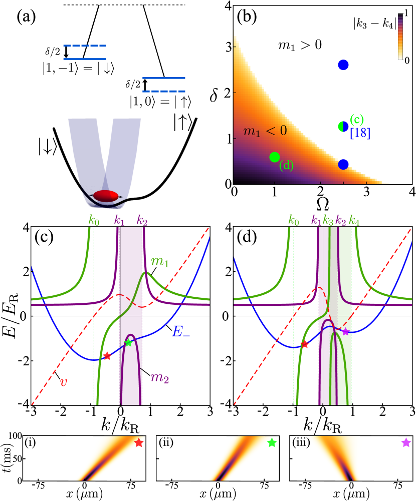
Figure 1: (Color online) (a) Schematic of the experimental configuration. The BEC initially resides at the bottom of the lower branch shaped by the spin-orbit coupling (see energy level diagram). The trap is then released in the $x$ dimension to let the BEC expand. (b) Parameter space for $m_{1}$, defined by the momentum range $|k_{3}-k_{4}|$ for which $m_{1}$ is negative. Blue dots: configurations considered in Khamehchi et al. (2017). Green dots: configurations explored here. (c) SOCBEC dispersion properties for $\Omega=2.5$, $\delta=1.36$, $k_{\mathrm{R}}=1$ (from Ref. Khamehchi et al. (2017)). Blue line: lower branch $E_{-}$. Green line: effective mass $m_{1}$. Purple line: effective mass $m_{2}$. Red dashed line: group velocity $v$. The lower branch presents a region with $m_{2}<0$, where $v$ decreases with increasing $k$. (d) As for (c), but $\Omega=1$, $\delta=0.7$, $k_{\mathrm{R}}=1$, $E_{-}$ has regions with both $m_{1}<0$ and $m_{2}<0$, and $v$ has opposite sign to the momentum. (i–iii) Examples of wave packet propagation, the coloured stars indicate where $E_{-}$ is excited.

The dispersion relation for the lower band for two sets of Raman laser parameters $k_{R}$, $\Omega$ and $\delta$, are shown as a blue line in Fig. 1(c, d). As both are clearly non-parabolic, it is important to consider both the first and second mass parameters, rather than only $m_{2}$ that was discussed in Ref. Khamehchi et al. (2017). The parameter space for $m_{1}$ is plotted in Fig. 1(b), where we have identified the sets of parameters considered in Ref. Khamehchi et al. (2017) as well as those of the present Letter. We emphasize that the dispersion relation in Fig. 1(c) is identical to one set of SOC parameters considered in Ref. Khamehchi et al. (2017).

We now focus on the properties of the lower branch. An inflection point of this branch corresponds to a change of sign of $m_{2}$, which becomes infinite at the points $k_{1,2}$ meaning that wave packets with this quasi-momentum do not diffuse Sup (a). Similarly, one can define the points $k_{0,3,4}$ at which the mass $m_{1}$ diverges Sup (a). Most of the dynamics can now be understood regarding only the $k$-dependent group velocity $v(k)$, directly shaped by $m_{1}$ and $m_{2}$ Sup (a). As can be seen in Fig. 1(c,d), the linear parts of the dispersion, when $m_{2}$ diverges at $k_{1,2}$, lead to a local minimum or maximum for the group velocity. Similarly, $v$ is zero when the dispersion is locally flat at the points $k_{0,3,4}$, and takes negative values between $k_{3}$ and $k_{4}$, where $m_{1}<0$. A negative $m_{1}$ here corresponds to the packet moving in the opposite direction to the applied impulse, thus reversing the sign of the group velocity. We show in Fig. 1(i-iii) typical examples of wave packet propagation when exciting the branch at different quasi-momenta.

For the dispersion shown in Fig. 1(c), consider applying an impulse to move from the red (i) to the green (ii) star, where $m_{2}<0$. The wave packet decelerates, but keeps propagating in the same direction. Conversely, for the dispersion shown in Fig. 1(d), applying an impulse to move from the red (i) to the purple star (iii) (where $v<0$), one sees that the wave packet not only slows down, but actually reverses direction. We have provided an online interactive plot of the dispersion as a function of its key parameters $\delta$, $\Omega$ and $k_{\mathrm{R}}$ Sup (b).

We now analyse one-dimensional simulations of the dynamics of SOCBEC expansion in the context of $m_{1}$ and $m_{2}$ using the experimental parameters for $\delta=1.36$ and $\Omega=2.5$ from Ref. Khamehchi et al. (2017); foo (a). The dynamics of a 1D BEC initially positioned at the bottom of the lower branch and released from a harmonic trap in one direction can be described by a single-band Gross-Pitaevskii equation:

$$i\partial_{t}\psi(x)=\mathscr{F}^{-1}_{x}[E_{-}(k)\psi(k)]+g|\psi(x)|^{2}\psi(x)\,,$$ (5)

where $E_{-}(k)$ is the lower branch dispersion derived in Eq. 4 and shown in Fig. 1(c), $\mathscr{F}^{-1}_{x}$ is the inverse Fourier transform, and $g$ the effective 1D interaction strength.

We initially focus on the linear dynamics by setting $g=0$ so that we can study the free wave packet propagation with this dispersion, for which only $m_{2}$ is negative.

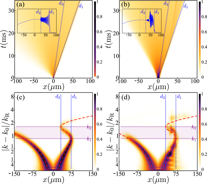
Figure 2: (Color online) BEC expansion with the SOC dispersion of Fig. 1(c). The first column shows the linear case with $g=0$, and the second column the interacting case. (a–b) Spacetime evolution of $|\psi(x,t)|^{2}$, with a condensate initial size of (a) $0.25\text{\,}\mathrm{\SIUnitSymbolMicro m}$, and (b) $5\text{\,}\mathrm{\SIUnitSymbolMicro m}$ Thomas-Fermi radius, obtained from the ground state of a $10^{4}$ particles BEC released from a $100\text{\,}\mathrm{Hz}$ trap. Insets: Density at $t=35$ ms. (c–d) Wavelet decomposition of $\psi(x)$ at $t=$35\text{\,}\mathrm{ms}$$. Vertical blue lines: limits of the diffusion cone in $x$. Purple horizontal lines: position of the inflection points in $k$. Red dashed curve: classical displacement $d(k)$ of each $k$-wave vector. An animation of this figure is provided as Supplementary Video S1 Sup (a).

We begin with a narrow Gaussian wave packet ($\sigma_{x}=$0.25\text{\,}\mathrm{\SIUnitSymbolMicro m}$$) centered at the minimum of the branch, so that its momentum spread encompasses the range $k_{1}$–$k_{2}$  foo (b). The spacetime evolution of the wave function $|\psi(x,t)|^{2}$ is plotted in Fig. 2(a) and shows a distinct interference pattern spatially confined in the diffusion cone defined by $d_{1,2}(t)=v(k=k_{1,2})t$. An enlightening method to visualise the self-interference effect is to plot the wave function density in the $x$-$k$ plane by performing the Wavelet Transform (WT) $\mathbb{W}(x,k)=(1/\sqrt{|k|})\int_{-\infty}^{+\infty}\psi(x)\mathcal{G}^{\ast}[(x-x_{0})/k]\mathrm{d}x$ Debnath and Shah (2015). Recent studies have shown that the WT can be applied to analyse complex interacting wave packets dynamics Baker et al. (2012); Colas and Laussy (2016). Unlike the usual Fourier transform based on the decomposition of the signal into a sum of delocalised functions (sine and cosine), the WT uses localised wavelets. Here we choose the Gabor wavelet family, with Gaussian-like functions $\mathcal{G}^{*}$, and a high central frequency ensuring good resolution near the inflection points in the dispersion Márk (1997). Further details regarding the WT for wave packets are described in the Supplementary Material Sup (a).

Figure 2(c) shows the wavelet energy density $|\mathbb{W}(x,k)|^{2}$ at $t=$35\text{\,}\mathrm{ms}$$. The inflection point momenta $k_{1,2}$ are indicated in $k$ (purple lines), and the boundaries $d_{1,2}$ of the diffusion cone in $x$ (blue lines). We also plot the displacement $d(k)=v(k)t$ associated with each $k$-wave vector (red dashed line). From this simple picture, one can now understand the origin of the self-interference effect: different wave vectors of the packet travel with the same velocity, hence overlapping in real space and interfering. This happens only when the wave packet spreads over an inflection point of the branch. This phenomenology is a universal consequence of the shape of the dispersion, and can therefore be equally encountered for exciton-polariton and atomic condensates, despite their operating time scales that differ by nine orders of magnitude.

Practically, it is challenging to form a SOCBEC with such a broad spread in momentum. One way to overcome this difficulty is to load the packet directly in the inflection points region by imparting it with the appropriate momentum. A second way, used in the experiment of Khamehchi et al. Khamehchi et al. (2017), is to release the BEC from the trap leading to a broadening of the wave packet in $k$-space due to the conversion of interaction energy to kinetic energy. This is an effective way to push some components of the wave packet into the negative $m_{2}$ region. Further details of this approach are presented in the Supplementary Material Sup (a).

Here we simulate the expansion dynamics of an interacting system initially in a $100\text{\,}\mathrm{Hz}$ harmonic trap with a Thomas-Fermi radius of 5 $\mu$m corresponding to approximately $10^{4}$ atoms. This is more tightly confined with fewer atoms than the experiment of Ref. Khamehchi et al. (2017), which had a trap frequency of $26\text{\,}\mathrm{Hz}$, $10^{5}$ atoms, and a Thomas-Fermi radius of $23$ $\mu$m, but enables a direct comparison with the $g=0$ case. The results for the spacetime density and WT are shown in Fig. 2(b,d). Here the interference only becomes visible after a finite time, which is that needed for the expansion of the wave packet to reach $k_{1}$. The presence of self-interference is again confirmed by the WT analysis in Fig. 2(d). Due to the interactions, the self-interference pattern differs slightly from the non-interacting case, and the energy density distribution gets spread around $d(k)$, since this curve accounts for the packet’s $k$-components displacement from $t=0$. The initial packet is here 20 times larger and only the low $k$-region is significantly populated at $t=0$. We provide analysis of the exact experimental situation of Khamehchi et al. Khamehchi et al. (2017) in the Supplementary Material Sup (a). Their configuration has a larger nonlinearity which results in the population of $k$-components above $k_{2}$, which travel with a velocity larger than $v(k_{1})$. This results in the density “leaking out” of the diffusion cone ($d_{1}$), and was previously identified as being due to dynamical instability Khamehchi et al. (2017). The limited diffusion of the condensate as shown in Fig. 2(b), which might appear as a “self-trapping” effect, can be overcome if high enough momenta ($k>k_{2}$) are reached, as is the case in Ref. Khamehchi et al. (2017).

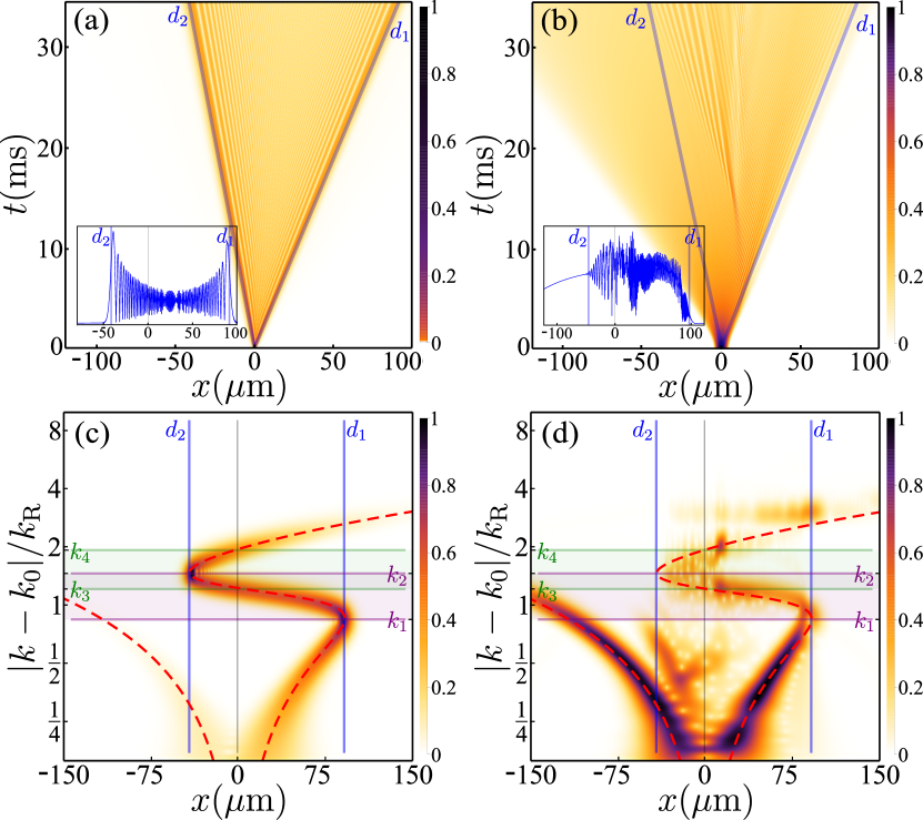
Figure 3: (Color online) BEC expansion with the SOC dispersion of Fig. 1(d) with both $m_{1}<0$ and $m_{2}<0$. The first column shows the noninteracting case with $g=0$, and the second column the interacting case. (a–b) Spacetime evolution of $|\psi(x,t)|^{2}$, with a condensate initial size of (a) $0.25\text{\,}\mathrm{\SIUnitSymbolMicro m}$, and (b) $5\text{\,}\mathrm{\SIUnitSymbolMicro m}$ Thomas-Fermi radius, obtained from the ground state of a $\approx 2.5\times 10^{4}$ particles BEC released from a $100\text{\,}\mathrm{Hz}$ trap. Insets: density at $t=35$ ms. (e–f) Wavelet decomposition of $\psi(x)$ at $t=$35\text{\,}\mathrm{ms}$$. The color code is the same as Fig. 2(c,d) with additional horizontal green lines delimiting the $m_{1}<0$ region. An animation of this figure is provided as Supplementary Video S2 Sup (a).

We now study the SOCBEC dispersion in a more interesting configuration that exhibits a stronger type of negative mass effect, shown in Fig. 1(d). This can be obtained by reducing the Raman coupling $\Omega$ and detuning $\delta$. In this case the mass $m_{1}$ is also negative in the momentum range $k_{3}$–$k_{4}$ for which $v<0$. Again, we first consider the non-interacting case ($g=0$), but this time with a Gaussian packet centered on $k=k_{2}$ with a width $\sigma_{x}=$0.25\text{\,}\mathrm{\SIUnitSymbolMicro m}$$. As shown in Fig. 3(a), the wave packet exhibits a double SIP effect during its propagation as the initial state spreads over both $k_{1}$ and $k_{2}$. The most notable feature is the position of the second SIP, whose diffusion is limited by $d_{2}=v(k_{2})t$ in the $x<0$ region, as $k_{3}<k_{2}<k_{4}$. The packet is now composed of two sub-packets, each carrying and propagating a SIP in opposite directions. This can be seen in the WT in Fig. 3(c), where we have added the boundaries $k_{3,4}$ (green lines) delimiting the $m_{1}<0$ region. One can see how the wavelet energy density in the momentum range $k_{3}$–$k_{4}$ is only displayed in the $x<0$ region. This corresponds to the packet’s $k$-components experiencing backward propagation.

The double SIP behaviour can also be observed in the expansion of an interacting BEC. We again begin with the condensate ground state in a $100\text{\,}\mathrm{Hz}$ trap with a Thomas-Fermi radius of $6\text{\,}\mathrm{\SIUnitSymbolMicro m}$, corresponding to $\approx 2.5\times 10^{4}$ atoms, leading to the population of higher momenta as compared to the previous case. As before, the SIP effect is present within the overall diffusing packet as can be seen in Fig. 3(b), and in the WT shown in Fig. 3(d), one can see that the SIP is “delayed” as compared to the non-interacting case. Time-animated videos of $|\psi(x,t)|^{2}$ with $|\mathbb{W}(x,k)|^{2}$ for both the linear and interacting cases as presented in Fig. 2 and 3 are provided in Ref. Sup (a). In experiments, translating optical lattices or Bragg pulses could be used to impart a momentum to the condensate in order to more clearly exhibit the SIP effect Hamner et al. (2015). Other nonlinear features like shock waves or soliton trains observed by Khamehchi et al. Khamehchi et al. (2017), may appear a posteriori as the self-interference process induces large oscillations of the condensate density, and thus provide a breeding ground for these excitations. In this experiment, both these linear and nonlinear effects are intertwined and cannot be clearly separated in the dynamics. The limited diffusion of the condensate, sometimes described as a nonlinear self-trapping effect in the literature Anker et al. (2005); Alexander et al. (2006); Xue et al. (2008), can instead be viewed in this case as a consequence of peculiar dispersion relations containing inflection points and regions of negative effective mass. Although the condensate diffusion is strongly affected, it is not bounded and normal diffusion can still occur as the dispersion returns to being parabolic at higher momenta.

In conclusion, we have shown that SOCBECs provide an excellent platform to engineer dispersion relations, allowing the creation of regions of negative effective mass for both parameters $m_{1}$ and $m_{2}$ that govern wave packet dynamics. The mass $m_{1}$ leads to a negative group velocity for a positive impulse, while the mass $m_{2}$ leads to self-interference in the wave packet. Self-interference alone is a direct consequence of the linear dynamics where dispersion relations contain inflection points. The nonlinearity of the BEC can further add to the phenomenology, in particular by populating such regions in the momentum space, and allowing self-interference to subsequently lead to the formation of solitons. The wave packet dynamics for which both mass parameters are negative is within reach of the SOCBEC platforms. This would result in the formidable phenomenology of moving an object in the direction opposite to which it was pushed.

I Introduction

In this Supplementary Material, we provide further details regarding the analysis and the expansion dynamics of the SOCBEC in the context of Self-Interfering Packets. In Section II we provide a detailed analytical analysis of the properties of the SOC dispersion. In Section III we describe the Wavelet Transform and its properties. In Section IV we present the energy transformations in the expansion of the interacting condensate, and we show the quantitative differences between the cases of parabolic and SOC dispersion. In Section V we directly apply our analysis to 1D simulations using identical parameters to the SOCBEC expansion dynamics presented by Khamehchi et al. [18]. Finally, Section VI describes the three videos accompanying this Supplementary Material to more clearly show the complex dynamics occurring in the SOCBEC. The Equations and Figures from the main text are here quoted with numbers whereas those from the Supplementary are prefixed by “S”.

II SOCBEC dispersion analysis

The inflection points of the SOCBEC dispersion relation identify the wavevectors $k_{1,2}$ where the effective mass $m_{2}$ is infinite. Their location can be found by solving $1/m_{2}=\partial_{k}^{2}E_{-}(k)=0$, giving the following result:

$$k_{1,2}=\frac{\delta}{2\gamma}\pm\sqrt{\left(\frac{m\Omega^{2}}{4\gamma\hbar}\right)^{\frac{2}{3}}-\left(\frac{\Omega}{2\gamma}\right)^{2}}\,.$$ (S1)

This expression also provides a condition on the existence of the inflection points in the dispersion relation, as the term under the square root of Eq. S1 has to be positive. Thus the dispersion relation possesses inflection points if:

$$\frac{\hbar^{2}k_{\mathrm{R}}^{2}}{2m}<\frac{\hbar\Omega}{4}\,.$$ (S2)

The points $k_{0,3,4}$ at which the effective mass $m_{1}$ diverges can be found by solving $\partial_{k}E_{-}(k)=v(k)=0$. The analytical expression for the group velocity is:

$$v=\frac{\hbar k}{m}-\gamma\bigg{/}\sqrt{\left(\frac{\Omega}{2k\gamma-\delta}\right)^{2}+1}\,.$$ (S3)

One can see that for $k\gg\Omega/\gamma$ the dispersion is parabolic again, and the velocity grows linearly with the momentum. Analytical expressions exist for the points $k_{0,3,4}$ but they are too cumbersome to reproduce here. The point $k_{0}$ corresponds to the bottom of the SOCBEC dispersion and always exist. The effective mass $m_{1}$ is negative between the points $k_{3}$ and $k_{4}$ (when they exist), which corresponds to a negative velocity $v$. Figure 1(b) of the main text summarizes the parameter space for which $m_{1}$ is positive or negative.

III Wavelet Transform

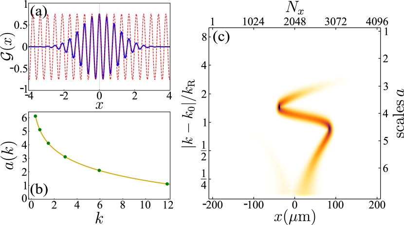
Figure S1: (a) Real part of the Gabor wavelet with a frequency $\omega=15$ (blue line) and its corresponding central frequency (dashed red line). (b) Log base 2 scaling between scales $a$ and momenta $k$. (c) Example of a scalogram showing the correspondences between: (i) Scales and momentum units; (ii) Number of points $N_{x}$ and space units.

The Wavelet Transform (WT) is commonly used in signal processing to obtain a signal representation both in time and frequency. This transform can also be applied to any complex wave function $\psi(x)$ in order to obtain its representation in both position $x$ and momentum $k$. The Wavelet Transform is:

$$\mathbb{W}(a,b)=(1/\sqrt{a})\int_{-\infty}^{+\infty}\psi(x)\mathcal{G}^{\ast}[(x-b)/a]\mathrm{d}x\,,$$ (S4)

where $a$ is the scale and $b$ the translation parameter. In physical terms, this quantity measures the cross-correlation between the wave function $\psi(x)$ and a wavelet $\mathcal{G}(x)$ that is scaled by $a$ and translated in space by $b$. This map $|\mathbb{W}(x,k)|^{2}$, also called scalogram, indicates the cross-correlation between position and momentum of the wave function. In the context of this paper, the WT is a remarkable tool to understand the complex wave packet dynamics that occurs in SOC systems. For this study, we work with the Gabor Wavelet:

$$\mathcal{G}(x)=\sqrt[4]{\pi}\exp(i\omega x)\exp(-x^{2}/2)\,,$$ (S5)

where $\omega$ is the wavelet’s frequency. The choice of this wavelet is natural since the Gabor wavelet—a Gaussian function with a well-defined frequency—corresponds to the archetype of a propagating quantum wave packet, embedding motion and diffusion in a transparent way [25]. The central frequency of the Gabor wavelet can be well approximated by:

$$f_{c}=\frac{2\pi(\omega+\sqrt{w^{2}+2})x}{4\pi}\,.$$ (S6)

The wavelet oscillations thus match with the oscillatory function $D=\pi^{-1/4}(\cos(f_{c}x)+i\sin(f_{c}x))$. In Fig. S1, the real part of the Gabor wavelet is plotted in blue and the function $\Re(D)$ in dashed red. In our numerical computations, we choose a relatively high wavelet frequency $\omega=15$ in order to obtain high cross-correlations in the inflection points region. We can now obtain the correspondence between the scales $a$ of the WT and the signal frequency (here the momentum) with:

$$k_{a}=\frac{f_{c}}{aN_{x}}\,,$$ (S7)

where $N_{x}$ is the number of points in the spatial grid, corresponding to the signal sampling rate. The scaling law that we use between scales and momentum is shown in Fig. S1(b). It follows a log base 2 scale, meaning that the momentum at the next scale is doubled (like the octaves in music). Low scales thus correspond to high momenta and vice versa. Here, each scale (octave) is also subdivided in 20 voices. An example of a scalogram showing the correspondence between scales (momenta) and grid points (position) is shown in Fig. S1(c).

IV Energy conversions of the condensate

The total energy functional for the Hamiltonian of Eq. (7) can be written as $E_{\mathrm{tot}}=E_{\mathrm{P}}+E_{\mathrm{NP}}+E_{\mathrm{int}}$, accounting for the kinetic energy from the parabolic and non-parabolic parts of the dispersion [see Eq. (4)], and for the interaction energy due to the nonlinear term of Eq. (7), respectively. The first and the last terms recover the total energy of the GPE in free space:

$$E_{\mathrm{P}}+E_{\mathrm{int}}=\int\left(\frac{\hbar^{2}}{2m}|\nabla\psi(x)|^{2}+\frac{g}{2}|\psi(x)|^{4}\right)\mathrm{d}x\,.$$ (S8)

The contribution from the non-parabolic part of the dispersion is most easily computed in momentum space:

$$E_{\mathrm{NP}}=\int-\frac{1}{2}\sqrt{\Omega^{2}(k-2k_{\mathrm{R}})^{2}+\delta^{2}}|\psi(k)|^{2}\mathrm{d}k\,.$$ (S9)

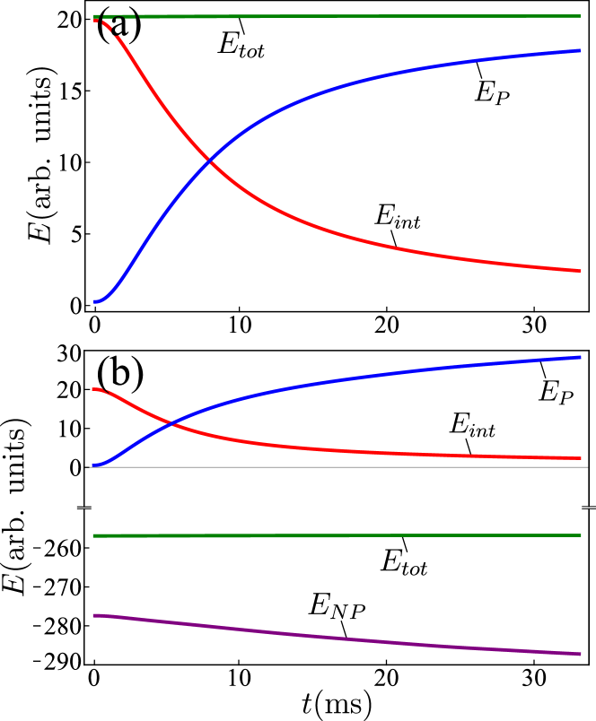
Figure S2: Energy conversions of the condensate (a) Parabolic dispersion case. At long times the interaction energy $E_{\mathrm{int}}$ is entirely converted into kinetic energy $E_{\mathrm{P}}$. (b) SOCBEC dispersion case corresponding to Fig. 2(b) of the main text. The interaction energy $E_{\mathrm{int}}$ is converted into both the parabolic $E_{\mathrm{P}}$ and non-parabolic $E_{\mathrm{NP}}$ parts of the kinetic energy.

In Fig. S2(a) we illustrate the conversion of the interaction energy into kinetic energy during the expansion of a single-component BEC described by a GPE with a parabolic dispersion. At long times the interaction energy is entirely converted into kinetic energy, and the condensate behaves like a noninteracting Schrödinger wave packet. The case corresponding to the SOCBEC dispersion described in Fig. 2(c) of the main text is presented in Fig. S2(b). The interaction energy is still converted to kinetic energy, but this time with a significant contribution from the non-parabolic part of the dispersion.

V Analysis of experiment by Khamehchi et al.

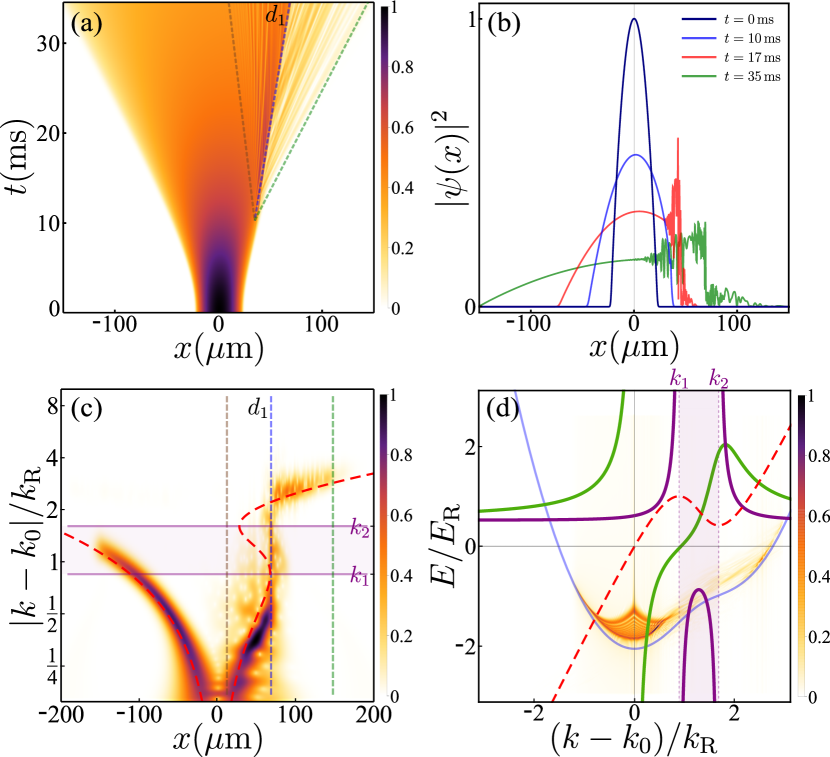
Figure S3: Analysis of the dynamics of SOCBEC expansion as studied by Khamehchi et al. [18]. $\Omega=2.5$, $\delta=1.36$, $k_{\mathrm{R}}=1$, $\omega=2\pi\times$26\text{\,}\mathrm{Hz}$$, Thomas-Fermi radius 23 $\mu$m. (a) Spacetime dynamics of the condensate density following release from the trap. The brown and green dashed lines indicate the boundaries of self-interference, while the blue dashed line separates two distinct regions. (b) Condensate density at $t=\{0,10,17,35\}$ ms after release. (c) Wavelet Transform of the condensate wave function at $t=35$ ms. The boundaries of self interference are indicated using the same line styles as in (a). (d) Blue line: Dispersion relation of the lower branch $E_{-}$. Green line: effective mass $m_{1}$. Purple line: effective mass $m_{2}$. Red dashed line: group velocity $v$. Overlaid is the condensate spectral density $|\psi(k,E)|^{2}$. An animation of this figure is provided as Supplementary Video 3.

In the main text of the paper by Khamehchi et al. [18], the authors present numerical results from three-dimensional simulations of the Gross-Pitaevskii equation for comparison with their experimental observations. In addition, in the supplemental material they show that one-dimensional simulations of a BEC with the same Thomas-Fermi radius exhibit very similar features [18]. In this section we perform a wavelet analysis of the equivalent one-dimensional simulations to demonstrate that the root cause of their observations is the SIP phenomenon.

Our simulations begin with the ground state of a SOCBEC with $\Omega=2.5$, $\delta=1.36$, $k_{\mathrm{R}}=1$ in a $\omega=2\pi\times$26\text{\,}\mathrm{Hz}$$ trap with a Thomas-Fermi radius of 23 $\mu$m, corresponding to approximately $10^{5}$ atoms. The spacetime evolution of the BEC density following release from the trap is shown in Fig. S3(a), with slices showing the condensate density at selected times in Fig. S3(b). The WT of the wave function taken at $t=t_{\textrm{max}}$ is shown in Fig. S3(c). The far-field of the wave function $\psi(x,t)$ can be computed by performing the Fourier Transform on both time and spatial coordinates, yielding the spectral density $|\psi(k,E)|^{2}$ and is shown in Fig. S3(d) overlaid with the dispersion relation for the system. This observable is easily measured experimentally for polariton systems where the photons leaking out of the cavity allow a continuous monitoring of the phase and density of the field. However such a measurement is challenging in atomic systems as the measurement of the density and phase of the condensate is generally destructive. Nonetheless, there is no barrier to determining the condensate spectral density in simulations.

From the spacetime density in Fig. S3(a) we can see two distinct regions of interference bounded on the outside by brown and green dashed lines, and separated in the middle by the blue dashed line labeled $d_{1}$. The delimitation lines of the interference areas are also shown on the WT in Fig. S3(c), where we can see that the “leaking part” previously identified by Khamehchi et al. [18] comes from the interference of $(k>k_{2})$-components (when $m_{2}>0$ again) with lower $k-$components. We can also see in the comparison of the spectral density with the dispersion in Fig. S3(d) that the field follows the dispersion again at $k>k_{2}$.

From this analysis we can see that the essential feature of the experiment of Khamehchi et al. [18] in comparison to the cases presented in the main text is a stronger nonlinearity, and a weaker initial confinement. This means it takes longer for the generation of the higher-$k$ components, and hence for the self-interference to occur. The stronger nonlinearity leads to a more significant blue shift, and results in a more complex interference pattern combined with the the generation of grey solitons.

VI Supplementary Videos

Three supplementary videos are provided with this material. The first two show the time-resolved SOCBEC dynamics in both the linear and interacting regimes, as observed directly through the wave packet motion in real space and the WTs. Supplementary Video S1 is for the SOC configuration of Khamehchi et al. [18] where only one mass parameter is negative, and corresponds to the results presented in Fig. 2. Supplementary Video S2 is for the SOC configuration of the main text where both masses parameters are negative, corresponding to the results presented in Fig. 3. Finally, Supplementary Video S3 shows the effect of the changing the strength of the nonlinearity on the SOCBEC dynamics corresponding to the experiment of Khamehchi et al. [18], and as presented here in Fig. S3. The movie is parameterised by the Thomas-Fermi radius of the BEC, and begins from weakly interacting system with a small nonlinearity, and ends with the parameters of Fig. S3.