Attack Potential in Impact and Complexity

Abstract.

Vulnerability exploitation is reportedly one of the main attack vectors against computer systems. Yet, most vulnerabilities remain unexploited by attackers. It is therefore of central importance to identify vulnerabilities that carry a high ‘potential for attack’. In this paper we rely on Symantec data on real attacks detected in the wild to identify a trade-off in the Impact and Complexity of a vulnerability, in terms of attacks that it generates; exploiting this effect, we devise a readily computable estimator of the vulnerability’s Attack Potential that reliably estimates the expected volume of attacks against the vulnerability. We evaluate our estimator performance against standard patching policies by measuring foiled attacks and demanded workload expressed as the number of vulnerabilities entailed to patch. We show that our estimator significantly improves over standard patching policies by ruling out low-risk vulnerabilities, while maintaining invariant levels of coverage against attacks in the wild. Our estimator can be used as a first aid for vulnerability prioritisation to focus assessment efforts on high-potential vulnerabilities.

1. Introduction

The identification of objective and readily available measures for vulnerability risk is a central part of the vulnerability mitigation process (Verizon-2014, ; PCI-DSS-DOC, ; SCAR-MELL-09-ESEM, ). Industry standards such as the Common Vulnerability Scoring System (CVSS) have been developed to create a common framework over which evaluate vulnerability severity and guide the vulnerability mitigation process (SCAR-MELL-09-ESEM, ); a CVSS assessment produces two final components:

1) The CVSS-vector, that contains the fine-grained information regarding the characteristics of the vulnerability. Among other values, the CVSS-vector provides information on the complexity of the vulnerability exploitation (in the metric Access Complexity), and its impact on the attacked system.

2) The CVSS-score, a final severity score that synthesises the information in the CVSS-vector in a single value between 0 and 10 (less severe to more severe).

The CVSS-score is widely used as a metric for vulnerability management; for example, PCI-DSS, the worldwide security standard for systems handling credit-card data, sets a ‘hard threshold’ for vulnerability patching at a CVSS score greater or equal to 4 (10 being the maximum) (PCI-DSS-DOC, ). Similarly, NIST’s SCAP standard uses the CVSS-score as the metric of reference for vulnerability assessment across industry sectors, including consumer systems (Scarfone-2010-SCAP, ).

Unfortunately, recent studies show that the CVSS-score does not correlate well with attacks in the wild, leading to sub-optimal vulnerability management policies (Allodi-2014-TISSEC, ; Christey-2013-BHUSA, ; Verizon-2014, ). This is particularly unfortunate as the CVSS score gives a clear, well-defined and readily available assessment of the vulnerability that can be used ‘out-of-the-box’ to take a first security decision on whether the vulnerability is (not) likely to represent a significant risk (chakradeo2013mast, ). This is especially relevant as recent empirical (Allodi-ESSOS-15, ) as well as analytical (Allodi-17-WAAM, ) findings indicate that most vulnerabilities remain unexploited by attackers. It is therefore especially important to devise measures that rule out ‘low-risk’ vulnerabilities to prioritize fine-grained assessments on high-potential vulnerabilities.

In this paper we investigate whether the information reported in the CVSS-vector may provide useful information, otherwise lost in the aggregate score, to estimate the attack potential of a vulnerability. Leveraging on real attack data from Symantec, we show the existence of a clear trade-off between exploitation complexity and impact in terms of number of expected attacks observed in the wild. We propose to leverage this trade-off to identify a new measure, ‘Attack Potential’, that can be readily estimated from the CVSS-vector and used as a measure of vulnerability prioritization next to the standard CVSS-score metric (e.g. in a standard security triage process (chakradeo2013mast, )). Building on top of previous related work (Allodi-2014-TISSEC, ), we show that patching policies based on our estimator show a comparable or better reduction in risk than current best practices by requiring an essentially halved workload in terms of patched vulnerabilities without losing ability of foiling attacks in the wild.

This paper is organised as follows: Section 2 introduces our datasets. Section 3 gives a first overview of exploits in Impact and Complexity. In Section 4 we introduce the Attack Potential measure, and in Section 5 we evaluate our estimator against real attacks in the wild. Section 6 discusses threats to validity; related work is presented in Section 7, and Section 8 concludes the paper.

2. Datasets

Our analysis is based on three datasets:

(1) The National Vulnerability Database (NVD) is usually considered the public universe of vulnerabilities held by NIST. Our NVD samples reports 49599 vulnerabilities (CVE identifiers).

(2) To approximate a collection of vulnerabilities used in the wild we have used Symantec’s AttackSignature and ThreatExplorer public data (SYM). It contains all entries identified as malware (local threats) or remote attacks (network threats) by Symantec’s commercial products. It reports 1277 vulnerabilities.

(3) Symantec’s WINE data sharing program (Dumitras-11-BADGERS, ) collects records of attacks for attack signatures and CVEs reported in SYM. Our WINE sample has been collected in Summer 2012 and reports 2M attacks detected between August 2009 and June 2012 against $10^{6}$ systems(Dumitras-11-BADGERS, ), and exploiting 408 vulnerabilities.

3. Explorative attack data analysis

CVSS classifies vulnerability Impact over an assessment of the classic Confidentiality, Integrity, Availability properties, expressed in terms of (C)omplete, (P)artial, (N)one losses. Figure 1 reports the trend in volumes of attacks per CIA impact type. Only CIA configurations for which there is an entry in WINE are reported (the interested reader can refer to (Allodi-2014-TISSEC, ) for a more detailed analysis of incidence of impact types on vulnerabilities and exploits).

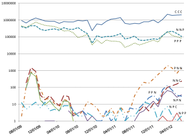
High Impact vulnerabilities are exploited several orders of magnitude more frequently than low Impact vulnerabilities.

Figure 1. Trends of attacks by impact type. Y-axis is in logarithmic scale

The Y-axis is in logarithmic scale. It is immediately evident that two levels of prevalence of CIA impacts in attacks can be identified: vulnerabilities with C,I,A assessment $<$C,C,C$>$$<$P,P,P$>$,$<$N,N,P$>$ are up to 5 orders of magnitude more exploited than most other impact types. $<$C,C,C$>$ and $<$P,P,P$>$ vulnerabilities are among the most targeted; this matches the observation that these impact types are among the most common overall in NVD (Allodi-2014-TISSEC, ). On the other hand, the high incidence of $<$N,N,P$>$ vulnerabilities in WINE does not match a high presence of this impact type in NVD (Allodi-2014-TISSEC, ). Further, it is useful to observe that $<$N,N,P$>$ vulnerabilities are more commonly exploited in the wild than $<$N,N,C$>$ vulnerabilities, despite a lower overall impact (Partial Availability as opposed to Complete Availability impact). Some light can be shed on the apparent mismatch between volume of attacks and relative impact of affected vulnerabilities by considering the Access Complexity levels reported in the NVD. We find that 95% of attacked $<$N,N,P$>$ vulnerabilities have a Low CVSS Access Complexity, and that more than 50% of $<$N,N,C$>$ vulnerabilities are scored as High or Medium complexity. This suggests that the combination of CVSS Impact and Access Complexity assessments may provide a useful first indicator of presence of exploit in the wild.

Trends of attacks in Impact and Complexity

Following official guidelines (Mell-2007-CMU, ), we categorise vulnerabilities by their impact and complexity over three levels for each metric: $HIGH,MEDIUM,LOW$. Vulnerability characteristics are identified in short by the tuple $<$AC=X,I=Y$>$, with $x$ and $y$ the assessments for the Access Complexity and Impact metrics respectively. Table 1 reports the relative fractions of vulnerabilities in SYM for each combination.

Table 1. Relationship between Access Complexity, Impact and presence of exploit.

Fraction of vulnerabilities exploited in the wild reported in SYMby Impact and Access Complexity. Low-complexity vulnerabilities are the most frequent ones. Medium-complexity vulnerabilities are only exploited when matched by a High Impact. High-complexity vulnerabilities are seldom exploited. Fractions in SYMare clearly different from those in NVD, indicating that the selection process of vulnerability exploits is not random.

Acc. Complexity	Impact	SYM	NVD
HIGH	HIGH	1.33%	0.92%
	MEDIUM	1.88%	1.89%
	LOW	1.02%	1.89%
MEDIUM	HIGH	32.50%	7.65%
	MEDIUM	3.60%	7.69%
	LOW	2.43%	14.83%
LOW	HIGH	18.09%	11.80%
	MEDIUM	22.55%	30.43%
	LOW	16.60%	22.90%

It is evident that Low complexity and Medium complexity, High impact vulnerabilities are over-represented in SYM with respect to NVD. For example, $<$AC=M, I=H$>$ vulnerabilities constitute 32.5% of vulnerabilites in SYM, whereas they represent only 7.65% of vulnerabilities in NVD. Similarly, $<$AC=M, I={M,L}$>$ vulnerabilities are under-represented in SYM with respect to occurrences in NVD.

In Figure 2 we report attack volumes in time aggregated by {complexity, impact} types. The Y-axis is in logarithmic scale. In the plot the $<$AC=M, I=L$>$ tuple is not reported as many data points in the time series are zeros.

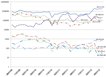
Vulnerabilities with a high impact-complexity trade-off are exploited orders of magnitude more often than other vulnerabilities. Medium Acc. Complexity vulnerabilities drive attacks only when matched by a high Impact.

Figure 2. Attacker trade-offs in Impact vs Complexity types. Y-axis is in logarithmic scale.

The great majority of exploited vulnerabilities are Low Access Complexity ones; among these, the most attacked are High Impact vulnerabilities. Medium Access Complexity vulnerabilities are massively exploited only if their impact on the victim systems is High. The resulting picture is therefore rather simple: the majority of exploits are for easy vulnerabilities to exploit, regardless of their Impact type. Medium complexity vulnerabilities are less targeted (by two orders of magnitude), and only if the exploitation impact is High. Essentially we can see that Low Complexity and High Impact vulnerabilities remain at large the favorite vector for attacks while the remaining Low Complexity or Medium Complexity but High Impact are still very popular albeit by varying degrees (oscillating in 1 order of magnitude below the top category). The other vulnerability types remain below at several orders of magnitude. This suggests that the combination of Access Complexity and Impact may help identifying useful measures for incidence of attacks.

4. Potential of attack

To more precisely describe the trends outlined in Section 3 we define $pA$ as an empirical measure of the potential of attack of a vulnerability over a set of vulnerable machines. Our $pA$ measure is specified as

(1) $$pA=log_{10}(A_{v})$$

where $A_{v}$ is the number of attacks observed in the wild for the vulnerability $v$. A $pA\ \text{of}\ 6$ corresponds to one million attacks in the wild in our sample (i.e. one per systems on average). A $pA=2$ indicates 100 recorded attacks. Figure 3

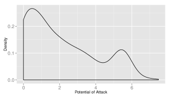
Figure 3. Probability density of $pA$ measures in WINE.

reports the probability density distribution of $pA$ for vulnerabilities reported in WINE. The x axis reports the $pA$ values and the y axis the incidence of each $pA$. $pA$ ranges in $[0..7.5]$. Its distribution spikes at $pA\approx 1$ and $pA\approx 6$. 50% of vulnerabilities are below a $pA$ of 1.6, and 75% below 3.4. This means that 50% and 75% of vulnerabilities receive respectively up to about 50 ($10^{1.6}$) and 2500 ($10^{3.4}$) attacks in the wild over the observation period.

Estimation of vulnerability attack potential

We exploit the impact-complexity effect described in Section 3 to estimate the volume of attacks that a vulnerability can potentially receive if an attack for it exists in the wild. Given the high incidence of unexploited vulnerabilities in the wild (Nayak-2014-RAID, ), a desirable property for our estimator is to maintain high true negative rates (something that the bare CVSS-score unfortunately does not do (Allodi-2014-TISSEC, )), whereas false positives can be ruled out by more fine-grained assessments later in a triage process (chakradeo2013mast, ). To build our estimator, we first assign to each Impact and Access Complexity value an ordinal value derived directly from the original CVSS v2 specification (Mell-2007-CMU, ). Table 2

Table 2. Scores by Impact and Access Complexity type. Values derived from the original CVSS v2 formula (Mell-2007-CMU, ).

Impact	Score
H	10
M	6
L	3

Acc. Complexity	Score
L	10
M	7
H	2

reports the assigned scores. Leveraging the logarithmic relation between attacks in the wild and CVSS measures, we define the estimated attack potential $E[pA]$ as:

(2) $$E[pA]=log_{10}(Impact)\times(Complexity)$$

The estimator in Eq. 2 will return values of $E[pA]\in[0,10]$. Because our WINE set is collected over $10^{6}$ machines (Dumitras-11-BADGERS, ), we define the following discrete levels:

• $5<E[pA]$: HIGH

• $3<E[pA]\leq 5$: MEDIUM

• $0\leq E[pA]\leq 3$: LOW

As an application example of our measure, Table 3

Table 3. $E[pA]$ estimates for vulnerabilities in the WINE sample.

Calculation of $E[pA]$ values for ten vulnerabilities in WINE. The estimator only need in input Access Complexity and Impact values from the CVSS-vector.

Vulnerability characteristics					$pA$		$E[pA]$
CVE	Sw	AC	Impact	#attacks	$pA$	Discrete $pa$	$E[pA]$	Discrete $E[pA]$	$E[pA]\approx pA$
CVE-2010-0806	internet_explorer	M	H	126765	5.1	HIGH	7	HIGH	✔
CVE-2009-3886	jre	L	M	427315	5.6	HIGH	8.4	HIGH	✔
CVE-2009-0075	internet_explorer	M	H	2803	3.4	MEDIUM	7	HIGH	$E[pA]>pA$
CVE-2008-5359	jdk	M	H	377324	5.6	HIGH	7	HIGH	✔
CVE-2008-0726	acrobat	M	H	246049	5.3	HIGH	7	HIGH	✔
CVE-2007-0038	windows_2000	M	H	2291	3.3	MEDIUM	7	HIGH	$E[pA]>pA$
CVE-2007-0015	quicktime	M	M	147857	5.1	HIGH	5.9	HIGH	✔
CVE-2005-4459	ace	L	H	4	0.6	LOW	10	HIGH	$E[pA]>pA$
CVE-2003-0109	windows_2000	L	M	203530	5.3	HIGH	8.4	HIGH	✔
CVE-1999-0749	windows_95	H	L	20	1.3	LOW	0.9	LOW	✔

reports the $pA$ and $E[pA]$ estimates for ten example vulnerabilities randomly sampled from WINE. Table 4

Table 4. $E[pA]$ and $pA$ discrete estimations.

Our $pA$ estimator conservatively estimates real volumes of attacks in the wild, and seldom under-estimates real $pA$ values. A low $E[pA]$ correctly matches a low-$pA$ vulnerability 67% of the time, whereas medium and high $E[pA]$ levels seem to consistently over-estimate low-$pA$ vulnerabilities.

		$E[pA]$
		HIGH	MEDIUM	LOW	Sum
$pA$	HIGH	70	13	3	86
	MEDIUM	62	2	7	71
	LOW	197	34	20	251
	Sum	329	49	30	408

reports overall results for the full WINE dataset. The estimator performs generally well, with only 6% of the assessments being under-estimations of real $pA$ (i.e. false negatives). Importantly, Table 4 shows that our estimator is a conservative one, in that when it does not match the correct $pA$ category, it over-estimates it. It therefore does not lead to ignoring vulnerabilities that should be treated. Among the false-negatives, 87% of the estimation error is limited to one level only on the discrete scale. Note that because all vulnerabilities considered in Table 4 have at least an exploit in the wild (as they are reported in WINE), the reported indicators do not represent real-world performance of the estimator. We give full a consideration of this in the next section.

5. An application to illustrative patching policies

To illustrate the practical application of our estimator to vulnerability management practices, we define a patching policy as a process that, given in input vulnerability data, outputs a Patch/NotPatch decision. A patching policy defines a threshold above which the Patch decision is triggered. We define the following policies:

• $All\ vulns$: no risk factor is identified; under this policy every vulnerability is patched.

• $CVSS\geq 4$: patches all vulnerabilities to which is assigned a CVSS score equal or higher than 4. This policy corresponds to the PCI DSS recommendation for management of credit card holders data (PCI-DSS-DOC, ).

• $COMPL=L$: patches ‘easy to exploit vulnerabilities’ with a CVSS Complexity assessment = $L$.

• $COMPL\leq M$: patches only ‘low hanging fruits’ vulnerabilities with a CVSS Complexity assessment either $L$ or $M$. High complexity vulnerabilities are ignored.

• $E[pA]=H$: accounts for vulnerabilities with a high estimated $pA$ ($E[pA]>5$).

5.1. Calculation of Risk Reduction

To evaluate the efficacy of the different patching policies, we compute the frequency with which each policy identifies a vulnerability in SYM. To evaluate each risk policy we randomly sample a vulnerability from NVD with the same characteristics in terms of software and year of disclosure as in SYM (Allodi-2014-TISSEC, ; Christey-2013-BHUSA, ). We then evaluate the count of sampled vulnerabilities that the policy marks as ‘high risk’ (i.e. above the threshold identified by the policy), and compare that to the vulnerability’s actual presence in SYM.

The output of our experiment is represented in Table 5.

Table 5. Output format of our experiment.

	$v\in{\textsf{S}YM}$	$v\not\in{\textsf{S}YM}$
Above Threshold	a	b
Below Threshold	c	d

The first row identifies the vulnerabilities that need be treated according to the decision variables. The risk entailed by selected vulnerabilities is computed on the first row, and is the ratio $R_{treated}=a/(a+b)$. The bottom row identifies the vulnerabilities that are not selected for treatment (below the identified threshold). The risk associated with the untreated vulnerabilities is the ratio $R_{untreated}=c/(c+d)$. The difference between the two is defined in the literature as risk reduction (RR) (Evans-1986-ACC, ). For a fixed number of vulnerabilities to patch, policies with a higher risk reduction identify a greater fraction of exploited vulnerabilities than policies with a lower risk reduction.

Formally, let $Attacked$ be the set of vulnerabilities for which attacks in the wild have been reported and $Selected$ the set of vulnerabilities above a policy’s threshold. The risk of treated (untreated) vulnerabilities for a patching policy $R_{treated}$ ($R_{untreated}$) and the risk reduction ($RR$) of a policy are defined as:

(3) $$R_{treated} = \frac{|Attacked\cap Selected|}{|Selected|}$$

(4) $$R_{untreated} = \frac{|Attacked\cap\neg Selected|}{|\neg Selected|}$$

(5) $$RR = R_{treated}-R_{untreated}$$

To implement the procedure we perform a bootstrapped case-control study as described in (Allodi-2014-TISSEC, ). Because different software types may lead to different attack frequencies, we identify four software categories in SYM to control for in our sample (Allodi-2013-IWCC, ; Christey-2013-BHUSA, ): IE, PLUGIN, PROD and WINDOWS. The classification is performed by manually assigning software names to a category and then using regular expressions to match each CVE to the respective category.

5.2. Risk reduction in the wild

With this formulation we can compare the policies identified in Section 5. Table 6

Table 6. Risk reduction and vulnerabilities to be considered per policy.

High risk reduction patching policies address a higher rate of exploited vulnerabilities by decreasing the rate of false positives. A policy based on our $E[pA]$ measure outperforms standard patching policies based on the sole CVSS-score or atomic values of the CVSS-vector.

Policy	#V	RR	C.I.
$All\ vulns$	14.380	-	-
$CVSS\geq 4$	13715	23.2%	21.2% - 24.5%
$Comp=L$	7552	13.0%	11.9% - 14.1%
$Comp\leq M$	13952	5.2%	2.6% - 6.3%
$E[pA]=H$	8308	26.8%	24.5% - 27.4%

reports the results of the analysis. The first row reports the results for the $All\ vulns$ policy. With reference to our NVD dataset sample, this would require analyzing more than 14 thousand vulnerabilities. Risk Reduction can not be computed for this policy as no vulnerability remains unselected for patching. Among all policies, $Comp=L$ and $Comp\leq M$ achieve the lowest risk reductions. This example is however useful in better illustrating the mechanism implemented by the RR metric. Whereas $Comp=L$ is a subset of $Comp\leq M$, its risk-reduction is significantly higher; this may result counter-intuitive as the latter contains all vulnerabilities included in the former. However, note that by including additional vulnerabilities that are not attacked, $Comp\leq M$ decreases $R_{treated}$, thus resulting in a lower overall $RR$. A high $RR$ results therefore from policies that well balance the risk of selected vulnerabilities with the ‘residual’ risk that characterizes unselected vulnerabilities. The largest risk reduction is achieved by the policy based on the impact-complexity trade-off ($RR=26.8\%$). The second largest RR is achieved by a policy based on PCI-DSS. The former requires to analyze 8.3 thousand vulnerabilities and the latter almost 14 thousand. From this perspective the policy $E[pA]=H$ seems to have the best trade-off: lowest number of vulnerabilities and best risk reduction.

Table 7 reports the risk reduction for the aggregate case and the experiment for the controls. Comparisons are by row.

Table 7. Risk reduction and workload, expressed in terms of no. vulnerabilities patched, for all controls.

Risk reduction and patching workload expressed in number of vulnerabilities to fix identified in NVD. The ordering of the risk reduction measure is essentially preserved over all software categories with the exception of WINDOWS, for which additional considerations apart from the technical characteristics of the vulnerability may need to be considered.

	Aggregate		IE		PLUGIN		WINDOWS		PROD
Policy	RR	#V	RR	#V	RR	#V	RR	#V	RR	#V
$All\ vulns$	-	14380	-	1223	-	588	-	490	-	895
$CVSS\ \geq 4$	23.2%	13715	-24.4%	1208	50.5%	577	3.4%	477	23.1%	867
$Comp=L$	13%	7552	7.9%	635	5.2%	230	-5.4%	236	11.4%	186
$Comp\leq M$	5.2%	13952	-37.4%	1197	36.4%	561	-23.0%	472	-15.5%	878
$E[pA]=H$	26.8%	8308	-28.2%	733	52.2%	449	-52.4%	389	21.3%	739

As we can see from the table, the relative ordering is essentially preserved for all control factors. With few exceptions, the preferred global policy remains the preferred one even when restricted to a specific software category. WINDOWS vulnerabilities are here an exception, showing that the trade-off may not be a good proxy for this software category and that other variables should be considered. IE shows mixed behavior with $E[pA]=H$ performing similarly to $CVSS\ \geq 4$, but worse than $Comp=L$ in terms of $RR$. A negative $RR$ indicates that the residual risk in the ‘untreated’ vulnerabilities is higher than the risk for the treated vulnerabilities.

5.3. $pA$ reduction in the wild

We now look at the the efficacy of each policy in reducing attacks in the wild. Table 8

Table 8. Workload and $pA$ reduction for all controls.

The policy based on the $E[pA]$ measure drastically decreases the fraction of vulnerabilities to consider for patching while foiling the vast majority of attacks in the wild (6.7 $pA$ points against an overall $pA$ of 6.8).

	Aggregate		IE		PLUGIN		WINDOWS		PROD
Policy	%V	$pA$	%V	$pA$	%V	$pA$	%V	$pA$	%V	$pA$
$All\ vulns$	100.0%	6.8	100.0%	5	100.00%	6.7	100.0%	6.1	100.0%	4.4
$CVSS\ \geq 4$	95.4%	6.8	98.8%	5	98.13%	6.7	97.3%	6.1	96.9%	4.4
$Comp=L$	52.5%	6.3	51.9%	-	39.12%	6.3	48.2%	5	20.8%	3.3
$Comp\leq M$	97.0%	6.8	97.9%	5	95.41%	6.7	96.3%	6.1	98.1%	4.4
$E[pA]=H$	57.8%	6.7	59.9%	5	76.36%	6.6	79.4%	6.1	82.6%	4.4

reports, for each control, the amount of patching work required relative to the total for that software category and the reduction in $pA$. By looking at the $pA$ and $\%V$ columns, it is possible to see that the $E[pA]=H$ patching policy achieves the lowest workload (requiring to patch only 58% of the original volume of vulnerabilities), and still fully addresses $pA$ in the wild throughout all software categories.

Further, the results reported in Table 8 can be used to validate the risk reduction measure introduced in (Allodi-2014-TISSEC, ). For RR to be a valid measure for patching policy effectiveness, there should be a correspondence between the level of RR and the policy’s effectiveness in the wild. In Table 6 the ‘PCI DSS’ policy (patch all vulnerabilities with $CVSS\geq 4$) and $E[pA]=H$ have the highest risk reductions (23% and 26% respectively). $Compl=L$ and $Comp\leq M$ showed a much lower RR, the latter being the worst. We find this same ordering to be preserved in the evaluation in the wild reported in Table 8. $E[pA]=H$ represents the best trade-off between workload and reduction in $pA$, while $Comp=L$ entails the lowest workload but at the price of a lower reduction in $pA$. Similar considerations can be done if we break down the analysis for the controls.

6. Threats to validity

External validity. WINE data is a representative sample of attacks detected in the wild against ‘user machines’. Our conclusions are therefore limited to systems of the same nature: different dynamics may hold for server machines or specialized systems. Internal validity. Volumes of attacks against vulnerabilities may change by geographical area. It is possible that some vulnerabilities attacked only in particular areas or affecting only particular systems of lower commercial interest for Symantec may not appear or are under-represented in our datasets. To address this, in our case-control study we control for possible factors for inclusion in SYM (Allodi-2014-TISSEC, ). Further refinements may be needed to safely narrow the scope of our conclusions down to specific user populations.

7. Related work

An analysis of the distribution of CVSS scores and subscores has been presented by Scarfone et al. in (SCAR-MELL-09-ESEM, ). Frei et al.’s (Frei-2006-LSAD, ) studied the life-cycle of a vulnerability from exploit to patch. Their dataset is a composition of NVD, OSVDB and ‘FVDB’ (Frei’s Vulnerability DataBase, obtained from the examination of security advisories for patches). The notion of vulnerability risk has been considered in (Allodi-2014-TISSEC, ), where the authors show that the CVSS score as an aggregate number is not a satisfactory risk metric for vulnerabilities. Holm et al. (holm2015expert, ) investigated through expert opinion which aspects of a vulnerability should be considered on top of the baseline CVSS assessment to better represent risk of exploit. The present work extends this line of research by showing that the inner assessments in the CVSS framework can be instrumental for vulnerability prioritisation. Other work focused on the volume of attacks in the wild recorded against vulnerabilities. Allodi showed in (Allodi-ESSOS-15, ) that vulnerability exploitation follows a heavy-tailed distribution, and that for some software types as little as 5% of attacked vulnerabilities represent 95% of the risk in the wild. Similarly, Nayak et al. (Nayak-2014-RAID, ) showed that attackers prefer certain vulnerabilities over others. Our work integrates these results by showing that part of the attacker’s decision process is influenced by a trade-off between the complexity and the impact of the vulnerability exploit.

8. Conclusions

In this paper we investigated trends in vulnerability attacks per CVSS Impact and Exploitability types. We find that there exists a clear-cut distinction in terms of attacks in the wild between low complexity, high impact vulnerabilities and high complexity, low impact vulnerabilities.

Leveraging this effect we build an estimator of the Attack Potential of a vulnerability that provides a first indicator of the risk of exploitation in the wild. The estimator presented in this work is straightforward to implement and can be used in foresight without pre-existing data on the volume of attacks in the wild for that vulnerability. We test our estimator against standard CVSS-based patching policies and show that it outperforms them in terms of foiled attacks and entailed workload. The Attack Complexity metric in the 3.0 release of CVSS reflects these observations.

References

- [1] L. Allodi. The heavy tails of vulnerability exploitation. In Proc. of ESSoS’15, 2015.
- [2] L. Allodi and F. Massacci. Comparing vulnerability severity and exploits using case-control studies. ACM Transaction on Information and System Security (TISSEC), 17(1), August 2014.
- [3] L. Allodi, F. Massacci, and J. Williams. The work-averse cyber attacker model. evidence from two million attack signatures. In Published in WEIS 2017. Available at https://ssrn.com/abstract=2862299, 2017.
- [4] L. Allodi, S. Woohyun, and F. Massacci. Quantitative assessment of risk reduction with cybercrime black market monitoring. In In Proc. of IWCC’13, 2013.
- [5] S. Chakradeo, B. Reaves, P. Traynor, and W. Enck. Mast: Triage for market-scale mobile malware analysis. In Proceedings of the sixth ACM conference on Security and privacy in wireless and mobile networks, pages 13–24. ACM, 2013.
- [6] S. Christey and B. Martin. Buying into the bias: why vulnerability statistics suck. https://www.blackhat.com/us-13/archives.html#Martin, July 2013.
- [7] T. Dumitras and D. Shou. Toward a standard benchmark for computer security research: The worldwide intelligence network environment (wine). In Proc. of BADEGRS’11, pages 89–96. ACM, 2011.
- [8] L. Evans. The effectiveness of safety belts in preventing fatalities. Accident Anal. & Prev., 18(3):229–241, 1986.
- [9] S. Frei, M. May, U. Fiedler, and B. Plattner. Large-scale vulnerability analysis. In Proc. of LSAD’06, pages 131–138. ACM, 2006.
- [10] H. Holm and K. K. Afridi. An expert-based investigation of the common vulnerability scoring system. Computers & Security, 53:18–30, 2015.
- [11] P. Mell, K. Scarfone, and S. Romanosky. A complete guide to the common vulnerability scoring system version 2.0. Technical report, FIRST, Available at http://www.first.org/cvss, 2007.
- [12] K. Nayak, D. Marino, P. Efstathopoulos, and T. Dumitraş. Some vulnerabilities are different than others. In Proc. of RAID’14, pages 426–446. Springer, 2014.
- [13] PCI. Pci dss requirements and security assessment procedures, version 2.0. https://www.pcisecuritystandards.org/documents/pci_dss_v2.pdf, 2010.
- [14] S. D. Quinn, K. A. Scarfone, M. Barrett, and C. S. Johnson. Sp 800-117. guide to adopting and using the security content automation protocol (scap) version 1.0. Technical report, NIST, 2010.
- [15] K. Scarfone and P. Mell. An analysis of cvss version 2 vulnerability scoring. In Proc. of ESEM’09, pages 516–525, 2009.
- [16] Verizon. Verizon 2014 pci compliance report. Technical report, Verizon Enterprise, 2014.