Quantum spin circulator in Y junctions of Heisenberg chains

Abstract

We show that a quantum spin circulator, a nonreciprocal device that routes spin currents without any charge transport, can be achieved in Y junctions of identical spin-$1/2$ Heisenberg chains coupled by a chiral three-spin interaction. Using bosonization, boundary conformal field theory, and density-matrix renormalization group simulations, we find that a chiral fixed point with maximally asymmetric spin conductance arises at a critical point separating a regime of disconnected chains from a spin-only version of the three-channel Kondo effect. We argue that networks of spin-chain Y junctions provide a controllable approach to construct long-sought chiral spin liquid phases.

Introduction.—The spin-$1/2$ Heisenberg chain represents an analytically accessible model of basic importance in condensed matter theory Gogolin et al. (2004). By now, many experimental and theoretical works have contributed to a rather complete understanding of this model, including the effects of boundaries and junctions of two chains Eggert and Affleck (1992). However, little attention has been devoted to quantum junctions formed by more than two Heisenberg chains. In fact, recent theoretical developments provide hints that interesting physics should be expected in that direction: First, multichannel Kondo fixed points have been predicted for junctions of anisotropic spin chains Tsvelik (2013); Crampé and Trombettoni (2013); Tsvelik and Yin (2013); Buccheri et al. (2015). Second, electronic charge transport through junctions of three quantum wires is governed by a variety of nontrivial fixed points which cannot be realized in two-terminal setups Nayak et al. (1999); Chen et al. (2002); Chamon et al. (2003); Barnabé-Thériault et al. (2005); Oshikawa et al. (2006); Hou and Chamon (2008); Giuliano and Sodano (2009); Agarwal et al. (2009); Bellazzini et al. (2009); Rahmani et al. (2012). As spin currents in antiferromagnets can be induced by spin pumping Cheng et al. (2014) or by the longitudinal spin-Seebeck effect Hirobe et al. (2016), it is both an experimentally relevant and fundamental question to determine nontrivial fixed points governing spin transport in junctions of multiple spin chains. In particular, we are interested in the possibility of realizing a circulator for spin currents. While circulators have been discussed for photons Scheucher et al. (2016); Lodahl et al. (2017); Chapman et al. (2017) and for quantum Hall edge states Viola and DiVincenzo (2014); Mahoney et al. (2017), we are not aware of existing proposals for spin circulators. Once realized, a spin circulator has immediate applications in the field of spintronics Wolf et al. (2001), which has recently turned to the study of charge-insulating antiferromagnetic materials Wadley et al. (2016); Jungwirth et al. (2016); Baltz et al. (2018).

In this paper, we study Y junctions of spin-$1/2$ Heisenberg chains coupled at their ends by spin-rotation [SU(2)] invariant interactions. We assume identical chains such that the junction is $\mathbb{Z}_{3}$-symmetric under a cyclic exchange. These conditions are respected by a chiral three-spin coupling $J_{\chi}$ [see Eq. (1) below], which breaks time reversal (${\cal T}$) symmetry and can be tuned from weak to strong coupling, e.g., by changing an Aharonov-Bohm flux Wen et al. (1989); Sen and Chitra (1995); Claassen et al. (2017). Apart from condensed matter systems, such Y junctions can also be studied in ultracold atom platforms Esslinger (2010), where Heisenberg chains Murmann et al. (2015); Boll et al. (2016); Endres et al. (2016) and multi-spin exchange processes Dai et al. (2017) have recently been realized. We use three complementary theoretical approaches, namely bosonization Gogolin et al. (2004), boundary conformal field theory (BCFT) Cardy (1986, 1989); Affleck and Ludwig (1991a, b); Affleck (1993), and density matrix renormalization group (DMRG) simulations White (1992); Schollwöck (2005).

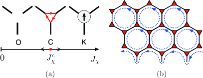
Figure 1: Y junction and network. (a) Schematic illustration of the phase diagram. For $J_{\chi}<J_{\chi}^{c}$, the system flows to open boundary conditions (O fixed point), while for $J_{\chi}>J_{\chi}^{c}$, the three-channel Kondo (K) point is approached. The two stable fixed points are separated by an unstable chiral (C) fixed point at $J_{\chi}=J_{\chi}^{c}$. (b) A network of Y junctions with uniform $J_{\chi}$ tuned to the C point realizes a chiral spin liquid.

Before entering a detailed discussion, we briefly describe our main conclusions, see Fig. 1(a): (i) We find two stable fixed points with emergent ${\cal T}$ symmetry. For small $|J_{\chi}|$, the renormalization group (RG) flow is towards the fixed point of open boundary conditions (O) representing disconnected chains. For large $|J_{\chi}|$, however, the system flows towards a spin-chain version of the three-channel Kondo fixed point Affleck and Ludwig (1991a), referred to as K point in what follows. So far only the two-channel Kondo effect with spin chains has been studied Eggert and Affleck (1992); Affleck (1993); Alkurtass et al. (2016). (ii) Both stable points are separated by an unstable chiral fixed point at intermediate coupling $|J_{\chi}|=J_{\chi}^{c}$, where the circulation sense is determined by the sign of $J_{\chi}$. DMRG simulations give $J^{c}_{\chi}/J=3.11(1)$, where $J>0$ is the bulk exchange coupling. (iii) Although the chiral point is unstable, it determines the physics over a wide regime of intermediate values of $J_{\chi}$. It then realizes an ideal spin circulator, where incoming spin currents are scattered in a chiral (left- or right-handed) manner around the Y junction. (iv) These findings provide a key step towards realizing a chiral spin liquid (CSL), an exotic phase of frustrated quantum magnets Kalmeyer and Laughlin (1987); Wen et al. (1989); Bauer et al. (2013, 2014); He et al. (2014); Gong et al. (2014); Gorohovsky et al. (2015); Bieri et al. (2015); Kumar et al. (2016). Our spin circulator provides a building block for network constructions of CSLs, cf. Fig. 1(b), where the chirality of each Y junction can be individually addressed.

Model.—We employ the Hamiltonian $H=H_{0}+H_{c}$, where $H_{0}=\sum_{j,\alpha}(J{\bf S}_{j,\alpha}\cdot{\bf S}_{j+1,\alpha}+J_{2}{\bf S}_{j,\alpha}\cdot{\bf S}_{j+2,\alpha})$ describes three ($\alpha=1,2,3$) identical semi-infinite Heisenberg chains (lattice sites $j=1,2,\ldots$). In numerical studies, it is convenient to tune the next-nearest-neighbor coupling $J_{2}=0.2412J$ to suppress logarithmic corrections present for $J_{2}=0$ Eggert and Affleck (1992). The part $H_{c}$ captures couplings between the boundary spin-$1/2$ operators ${\bf S}_{\alpha}\equiv{\bf S}_{j=1,\alpha}$. We require $H_{c}$ to preserve spin-SU(2) invariance and $\mathbb{Z}_{3}$ symmetry under cyclic chain exchange, $\alpha\to\alpha+1$ with ${\bf S}_{\alpha=4}={\bf S}_{1}$. These conditions allow for a ${\cal T}$-breaking three-spin coupling $J_{\chi}$,

$$H_{c}=J_{\chi}\hat{C},\qquad\hat{C}={\bf S}_{1}\cdot({\bf S}_{2}\times{\bf S}_{3}),$$ (1)

where $\hat{C}$ is the scalar spin chirality of the boundary spins Wen et al. (1989). We note that $J_{\chi}$ breaks reflection (${\cal P}$) symmetry, defined as exchange of chains $1$ and $2$, but $H$ is invariant under the composite ${\cal PT}$ symmetry. The $J_{\chi}$ interaction could be realized as an effective Floquet spin model for Mott insulators pumped by circularly polarized light Claassen et al. (2017). In principle, the ratio $J_{\chi}/J$ can be made arbitrarily large by varying bulk and boundary parameters independently. The above symmetries also allow for a $\mathcal{T}$-invariant boundary exchange coupling term, $J^{\prime}\sum_{\alpha}{\bf S}_{\alpha}\cdot{\bf S}_{\alpha+1}$. However, since $J^{\prime}$ does not qualitatively change our conclusions, we set $J^{\prime}=0$ below SM .

Weak coupling.—Let us start with the weak-coupling limit, $|J_{\chi}|\ll J$. In the low-energy continuum limit and for decoupled chains, spin operators take the form ($x=ja$ with lattice constant $a$) Gogolin et al. (2004)

$${\bf S}_{\alpha}(x)={\bf J}_{L,\alpha}(x)+{\bf J}_{R,\alpha}(x)+(-1)^{j}{\bf n}_{\alpha}(x),$$ (2)

where chiral spin currents ${\bf J}_{L/R,\alpha}(x)$ represent the smooth part and ${\bf n}_{\alpha}(x)$ the staggered magnetization. Using Abelian bosonization, we express these operators in terms of chiral bosons $\varphi_{L/R,\alpha}(x)$ or, equivalently, dual fields $\phi_{\alpha}(x)=\left(\varphi_{L,\alpha}-\varphi_{R,\alpha}\right)/\sqrt{2}$ and $\theta_{\alpha}(x)=\left(\varphi_{L,\alpha}+\varphi_{R,\alpha}\right)/\sqrt{2}$ Gogolin et al. (2004). With the non-universal constant $A\sim 1/a$ and $\nu=L/R=+/-$, one finds

$$J_{\nu,\alpha}^{z}(x) = \frac{\nu}{\sqrt{4\pi}}\partial_{x}\varphi_{\nu,\alpha},\quad J^{\pm}_{\nu,\alpha}(x)=\frac{1}{2\pi a}e^{\pm i\sqrt{4\pi}\varphi_{\nu,\alpha}},$$

$$n^{z}_{\alpha}(x) = A\sin[\sqrt{2\pi}\phi_{\alpha}],\quad n_{\alpha}^{\pm}(x)=Ae^{\pm i\sqrt{2\pi}\theta_{\alpha}}.$$ (3)

For $J_{\chi}=0$, open boundary conditions at $x=0$ are imposed by writing $\varphi_{R,\alpha}(x)=\varphi_{L,\alpha}(-x)+\varphi_{0}$ Gogolin et al. (2004), where SU(2) invariance requires $\varphi_{0}=0$ or $\varphi_{0}=\sqrt{\pi}$. In terms of SU(2) currents, we have $\mathbf{J}_{R,\alpha}(x)=\mathbf{J}_{L,\alpha}(-x)$. The effective low-energy Hamiltonian can be written as $H_{0}\simeq(2\pi v/3)\sum_{\alpha}\int_{-\infty}^{+\infty}dx\,\mathbf{J}_{L,\alpha}^{2}$, where $v\approx 1.17Ja$ Eggert and Affleck (1992) is the spin velocity for $J_{2}=0.2412J$. This model has central charge $c=3$ corresponding to three decoupled SU(2)₁ Wess-Zumino-Novikov-Witten (WZNW) models Gogolin et al. (2004); Affleck and Haldane (1987). We can then analyze the perturbations to the O point that arise for $|J_{\chi}|\ll J$. Boundary spin operators follow from Eq. (2) as ${\bf S}_{\alpha}\propto{\bf J}_{L,\alpha}(0)$ Eggert and Affleck (1992). The three-spin interaction $\sim J_{\chi}{\bf J}_{L,1}(0)\cdot[{\bf J}_{L,2}(0)\times{\bf J}_{L,3}(0)]$ has scaling dimension three and is irrelevant. In fact, it is more irrelevant than the leading $\mathcal{T}$-invariant perturbation $\sum_{\alpha}{\bf J}_{L,\alpha}(0)\cdot{\bf J}_{L,\alpha+1}(0)$ (dimension two), which is generated by the RG to second order in $J_{\chi}$.

Strong coupling.—Next, we address the limit $|J_{\chi}|\gg J$. For $J=0$, one can readily diagonalize the three-spin Hamiltonian $H_{c}$ Wen et al. (1989). The ground state of $H_{c}$ is twofold degenerate and, assuming $J_{\chi}>0$, has eigenvalue $-\sqrt{3}/4$ of $\hat{C}$. In the $|S_{1}^{z},S_{2}^{z},S_{3}^{z}\rangle$ boundary spin basis, the ground state with eigenvalue $M=+1/2$ of $\sum_{\alpha}S^{z}_{\alpha}$ is given by

$$|+\rangle=\frac{i}{\sqrt{3}}\left(|\downarrow\uparrow\uparrow\rangle+\omega|\uparrow\uparrow\downarrow\rangle+\omega^{2}|\uparrow\downarrow\uparrow\rangle\right),\quad\omega=e^{2\pi i/3}.$$ (4)

The $|-\rangle$ state with $M=-1/2$ follows by ${\cal PT}$ conjugation. All other states involve an energy cost of order $J_{\chi}$. For finite $J\ll J_{\chi}$, the low-energy physics therefore involves an effective spin-$1/2$ operator ${\bf S}_{\rm imp}$ acting in the $\{|+\rangle,|-\rangle\}$ subspace. By projecting $H$ onto this subspace, we arrive at a spin-chain version of the three-channel Kondo model,

$$\tilde{H}=H_{0}+J_{K}{\bf S}_{\rm imp}\cdot\sum_{\alpha}\left[{\bf S}_{2,\alpha}+(J_{2}/J){\bf S}_{3,\alpha}\right],$$ (5)

where $J_{K}\simeq J/3$. Since ${\bf S}_{\rm imp}$ is built from the original boundary spins ${\bf S}_{j=1,\alpha}$, the latter disappear from $H_{0}$ and the boundary is now at site $j=2$. The exchange coupling $J_{K}$ is marginally relevant. As a consequence, Kondo screening processes drive the system towards a strong-coupling fixed point identified with the K point. The physics of the K point is realized at energy scales below the Kondo temperature $T_{K}\sim Je^{-1/\lambda_{0}}$, where $\lambda_{0}\approx J_{K}a/(2\pi v)$ Laflorencie et al. (2008). Although the projected Hamiltonian in Eq. (5) lacks $\mathcal{T}$-breaking interactions, such interactions are generated by a Schrieffer-Wolff transformation to first order in $J/J_{\chi}$. However, they turn out to be irrelevant SM . Before analyzing the K point using BCFT, we turn to the critical point separating the stable O and K points.

Chiral fixed point.—We define the chirality $\hat{C}_{j}=\mathbf{S}_{j,1}\cdot(\mathbf{S}_{j,2}\times\mathbf{S}_{j,3})$ for three spins at site $j$ in different chains, cf. Eq. (1). In the continuum limit, the most relevant contribution to $\hat{C}_{j}$ stems from the staggered magnetization, $\hat{C}_{j}\sim\mathbf{n}_{1}(x)\cdot[\mathbf{n}_{2}(x)\times\mathbf{n}_{3}(x)]$. Energetic considerations suggest that $J_{\chi}\neq 0$ should favor a fixed point in which $\hat{C}=\hat{C}_{1}$ acquires a nonzero expectation value. This happens if we impose

$$\varphi_{R,\alpha\pm 1}(x)=\varphi_{L,\alpha}(-x)+\varphi_{0}.$$ (6)

As for the O point, SU(2) invariance requires $\varphi_{0}=0$ or $\varphi_{0}=\sqrt{\pi}$. Equation (6) implements ideal chiral boundary conditions for the spin currents,

$$\mathbf{J}_{R,\alpha\pm 1}(0)=\mathbf{J}_{L,\alpha}(0).$$ (7)

We refer to the corresponding fixed points as C_±, respectively.

Ideal spin circulator.—To see that the C_± points realize an ideal spin circulator, we consider the linear spin conductance tensor (with arbitrary $y>0$ and $\omega\to i0^{+}$) Meier and Loss (2003); Oshikawa et al. (2006)

$$\mathbb{G}_{\alpha\alpha^{\prime}}^{bb^{\prime}}=-\frac{(g\mu_{B})^{2}}{\hbar L\omega}\intop_{0}^{L}dx\intop_{-\infty}^{\infty}d\tau\,e^{i\omega\tau}\left\langle{\cal T}_{\tau}J_{\alpha}^{b}(x,\tau)J_{\alpha^{\prime}}^{b^{\prime}}(y,0)\right\rangle,$$ (8)

which determines the spin current in chain $\alpha$ with polarization direction $\hat{e}_{b=x,y,z}$ in response to a spin chemical potential Jungwirth et al. (2016); Baltz et al. (2018) applied in chain $\alpha^{\prime}$ with polarization $\hat{e}_{b^{\prime}}$. Here $g$ denotes the gyromagnetic ratio, $\mu_{B}$ the Bohr magneton, $L$ the chain length, ${\cal T}_{\tau}$ the imaginary-time ($\tau)$ ordering operator, and the spin current density is ${\bf J}_{\alpha}={\bf J}_{R,\alpha}-{\bf J}_{L,\alpha}$, cf. Eq. (2). Using the boundary conditions in Eq. (7), we obtain from Eq. (8) the maximally asymmetric tensor

$$\mathbb{G}_{\alpha\alpha^{\prime}}^{bb^{\prime}}=\frac{(g\mu_{B})^{2}}{2\pi\hbar}\delta^{bb^{\prime}}\left(\delta_{\alpha,\alpha^{\prime}}-\delta_{\alpha\pm 1,\alpha^{\prime}}\right)\qquad\text{(for C${}_{\pm}$)}.$$ (9)

Right at the C₊ or C_- point, an incoming spin current is therefore completely channeled into the adjacent chain $\alpha\pm 1$, cf. Fig. 1, without polarization change. The Y junction then represents an ideal spin circulator.

Realizing the chiral point.—It remains to show that the C_± points can be realized at intermediate $J_{\chi}$. We first approach the problem from the weak coupling side. Despite being energetically favored by $J_{\chi}\neq 0$, the C_± points must be unstable since the O point is stable for $|J_{\chi}|\ll J$. Indeed, a relevant boundary perturbation, $H_{1}$, is generated by the three-spin coupling when using Eq. (2) and imposing either of the conditions (6),

$$H_{1}=\lambda_{1}\sum_{\alpha}\cos\left\{\sqrt{\pi}\left[\varphi_{L,\alpha}(0)-\varphi_{L,\alpha+1}(0)\right]\right\}.$$ (10)

Using bosonization, we find $\lambda_{1}<0$ and $|\lambda_{1}|\propto|J_{\chi}|$ for $|J_{\chi}|\ll J$. The physical process behind t his dimension-$1/2$ operator is the backscattering of spin currents Oshikawa et al. (2006). For $\lambda_{1}<0$, the RG flow approaches $\lambda_{1}\to-\infty$ at low energies. Pinning the boson fields to the respective cosine minima in Eq. (10) takes the system back to the O point. Since at weak coupling there is only one relevant perturbation allowed by $\mathbb{Z}_{3}$ symmetry, the C point can be reached by fine tuning a single parameter $\lambda_{1}$, e.g., by increasing $J_{\chi}$. Let us assume that there is a critical value $J_{\chi}^{c}$ such that $\lambda_{1}(J_{\chi}^{c})=0$. For $J_{\chi}>0$ ($J_{\chi}<0$), this putative critical point corresponds to the C_- (C₊) point.

Now consider approaching the C point from the strong coupling side. For $J_{\chi}>J_{\chi}^{c}$, the relevant coupling constant becomes positive, $\lambda_{1}>0$, and the RG flow approaches $\lambda_{1}\to+\infty$. The pinning conditions now involve a $\pi$-phase shift for the cosine terms in Eq. (10) as compared to $J_{\chi}<J_{\chi}^{c}$. For the total magnetization $S^{z}_{\rm tot}=-\sum_{\alpha}[\varphi_{L,\alpha}(0)-\varphi_{R,\alpha}(0)]/\sqrt{2\pi}$, this shift means that an effective spin-$1/2$ degree of freedom has been brought from infinity to the boundary. This is precisely what we expect from the formation of the impurity spin in the strong coupling regime. The coupling of the impurity spin to the bulk allows for a second dimension-$1/2$ boundary operator, $H_{2}=\lambda_{2}\mathbf{S}_{\text{imp}}\cdot\sum_{\alpha}\tilde{\mathbf{n}}_{\alpha}(0)$, where $\tilde{\mathbf{n}}_{\alpha}$ is the staggered magnetization after imposing Eq. (6). The flow of $\lambda_{1}$ and $\lambda_{2}$ to strong coupling leads to a fixed point where the impurity spin is overscreened by the three chains, which we identify with the K point.

Since $\lambda_{1}$ vanishes at the critical point, the effects of the dimension-$1/2$ perturbations are felt only when the renormalized couplings at energy scale ${\cal E}$ become of order one. We thus obtain a wide quantum critical regime, ${(1-J_{\chi}/J_{\chi}^{c})^{2}}\lesssim{\cal E}/J\ll 1$, where the physics is governed by the C point. Related but different chiral points have been discussed for electronic Y junctions Oshikawa et al. (2006). The latter are stable for attractive electron-electron interactions and the asymmetry of the charge conductance tensor depends on the interaction strength. By contrast, our C point is unstable, but due to SU(2) symmetry the spin conductance (9) is universal and maximally asymmetric.

BCFT approach.—A spin-$1/2$ impurity coupled with equal strength to the open ends of two spin chains realizes a spin version of the two-channel Kondo effect Eggert and Affleck (1992); Affleck (1993); Alkurtass et al. (2016). Here we develop a BCFT approach and extend this analogy to three channels. We employ the conformal embedding SU(2)${}_{3}\times\mathbb{Z}_{3}^{(5)}$, whereby the total central charge $c=3$ is split into a SU(2)₃ WZNW model (with $c=9/5$), representing the spin degree of freedom, and a parafermionic $\mathbb{Z}_{3}^{(5)}$ CFT (with $c=6/5$) Zamolodchikov and Fateev (1985); Fateev and Zamolodchikov (1987); Frenkel et al. (1992); Totsuka and Suzuki (1996); Affleck et al. (2001), representing the “flavor” (i.e., channel) degree of freedom.

The RG fixed points are characterized by conformally invariant boundary conditions Cardy (1986, 1989); Affleck and Ludwig (1991a). The spectrum of the theory is encoded by the partition function $Z_{\text{AB}}$ on the cylinder with boundary conditions A and B. For instance, $Z_{\text{OO}}$ represents the partition function with open boundary conditions at both ends. Partition functions with other boundary conditions can be generated via fusion Cardy (1989). The boundary operators that perturb the K point can be determined using double fusion with the spin-$1/2$ primary in the SU(2)₃ sector Affleck and Ludwig (1991b); Affleck (1993). The leading irrelevant operator is the Kac-Moody descendant $\bm{\mathcal{J}}_{-1}\cdot\bm{\phi}_{1}$, where $\bm{\mathcal{J}}$ is the SU$(2)_{3}$ current and $\bm{\phi}_{1}$ is the spin-$1$ primary. This $\mathcal{T}$-invariant operator has scaling dimension $\Delta=7/5$, as in the free-electron three-channel Kondo model Affleck and Ludwig (1991a, b). Similarly, the leading chiral boundary operator at the K point is the dimension-$8/5$ field of $\mathbb{Z}_{3}^{(5)}$ Fateev and Zamolodchikov (1987). Moreover, the effective Hamiltonian at the K point includes only irrelevant boundary operators in the presence of cyclic exchange symmetry SM .

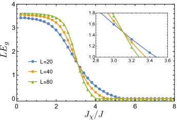
Figure 2: DMRG results for the finite-size energy gap $E_{g}$, rescaled by the chain length $L$, vs $J_{\chi}/J$ for several $L$. The inset highlights the crossing that determines the critical point.

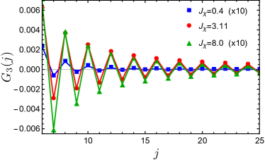
Figure 3: Three-spin correlations, $G_{3}(j)$, vs distance from the junction for $L=80$ and three values of $J_{\chi}$. The data for $J_{\chi}=0.4\,J$ and $J_{\chi}=8\,J$ are scaled up by a factor 10. Solid lines represent fits to a power-law decay.

Table 1: Exponent $\nu(J_{\chi})$ obtained by fitting the decay of $G_{3}(j)$ in the interval $8\leq j\leq L/2$. The extrapolated value follows from a second-order-polynomial fit. The last column shows the predictions for the O, C, and K points, respectively.

$J_{\chi}/J$		$L=40$	$L=60$	$L=80$	Extrap.	Expected
$0.4$		$3.56$	$3.51$	$3.49$	$3.45$	$3.5$
$3.11$		$1.89$	$1.79$	$1.74$	$1.59$	$1.5$
$8$		$2.31$	$2.22$	$2.18$	$2.08$	$2.1$

DMRG results.—We now describe numerical results for Y junctions with chain length $L$ using the DMRG algorithm by Guo and White Guo and White (2006), which works efficiently for open boundary conditions at $j=L$. First, we look for the critical point by analyzing the finite-size gap $E_{g}$ between the lowest-energy state with $S^{z}_{\text{tot}}=\sum_{j,\alpha}S^{z}_{j,\alpha}=0$ and the one with $S^{z}_{\text{tot}}=1$. For large $L$, at weak coupling we expect $E_{g}$ to approach the singlet-triplet gap of decoupled chains (O point), $E_{g}=\pi v/L$. On the other hand, at strong coupling, the BCFT approach predicts (through the partition function $Z_{\text{KO}}$ SM ) that the ground state is a triplet and hence $E_{g}$ should vanish identically. We indeed observe a ($L$-dependent) level crossing between a singlet ground state for small $J_{\chi}$ and a triplet for large $J_{\chi}$, see Fig. 2. The critical point is then determined from the crossing of the $LE_{g}$ vs $J_{\chi}$ curves for $40\leq L\leq 80$, resulting in $J_{\chi}^{c}/J=3.11(1)$.

Next, we calculate the three-spin ground-state correlation function $G_{3}(j)=\langle\hat{C}_{j}\rangle=\langle\mathbf{S}_{j,1}\cdot(\mathbf{S}_{j,2}\times\mathbf{S}_{j,3})\rangle$. At the C point, the long-distance decay of $G_{3}(j)$ is governed by the bulk scaling dimension of $\hat{C}_{j}$, where our BCFT predicts $G_{3}(j)\sim(-1)^{j}j^{-\nu_{\text{C}}}$ with $\nu_{\text{C}}=3/2$. Near the $\mathcal{T}$-symmetric O and K points, the leading chiral boundary operator has dimension $\Delta_{\rm O}=3$ and $\Delta_{\rm K}=8/5$, respectively. Standard perturbation theory around these fixed points yields $G_{3}(j)\sim(-1)^{j}j^{-\nu_{\text{O,K}}}$ with $\nu_{\text{O}}=7/2$ and $\nu_{\text{K}}=21/10$, respectively. Our DMRG results for $G_{3}(j)$ are shown in Fig. 3. First, we note that $G_{3}(j)$ has much larger magnitude and decays more slowly at the critical point. Fitting the numerical results to a power law expression with smooth and staggered parts yields the exponent $\nu(J_{\chi})$ of the dominant staggered term as listed in Table 1. For the fit, we only took into account data for $G_{3}(j)$ with $8\leq j\leq L/2$ in order to avoid both the non-universal short-distance behavior and effects due to the open boundary at $j=L$. (Results for $\nu(J_{\chi})$ are robust under changes of the fitting interval SM .) Our DMRG results in Table 1 agree well with the analytical predictions. The deviation is most significant at the C point, where one however also observes the strongest finite-size effects. We emphasize that the DMRG results show a slow decay of $G_{3}(j)$ over a wide region around the critical point.

Conclusions and Outlook.—We have demonstrated that a Y junction of Heisenberg chains acts as a quantum spin circulator in the vicinity of a critical point reached by tuning the three-spin interaction $J_{\chi}$. In addition to applications as a nonreciprocal device for pure spin transport, this spin circulator can be used for constructing two-dimensional networks realizing CSL phases, where the chirality of each node can be independently tuned Claassen et al. (2017). In fact, such an approach could allow for the systematic design of synthetic quantum materials harboring CSL phases. For instance, the network with uniform chirality shown in Fig. 1(b) has spin modes circulating in closed loops in the bulk. The bulk quasiparticles can be defined from the spin-1/2 field of the chiral WZNW model in each loop Gorohovsky et al. (2015) and have a finite gap due to the finite length of the loops. In addition, there is a gapless chiral edge mode with quantized spin conductance, cf. Fig. 1(b). This corresponds to the properties of the Kalmeyer-Laughlin CSL, a topological phase equivalent to a bosonic fractional quantum Hall system Kalmeyer and Laughlin (1987); Bauer et al. (2014). Furthermore, one can consider networks with alternating sign of $J_{\chi}$, i.e., staggered chirality between the nodes. This may shed light on the much less understood gapless CSLs with spinon Fermi surfaces Bauer et al. (2013); Bieri et al. (2015).

Appendix A Supplemental Material for “Quantum spin circulator in Y junctions of Heisenberg chains”

A.1 1. Effective Hamiltonian in the strong coupling limit

We consider the Hamiltonian for three boundary spins:

$$H_{c}=J^{\prime}\sum_{\alpha}\mathbf{S}_{\alpha}\cdot\mathbf{S}_{\alpha+1}+J_{\chi}\mathbf{S}_{1}\cdot(\mathbf{S}_{2}\times\mathbf{S}_{3}).$$ (11)

Here we have included the exchange coupling $J^{\prime}$ for a more general discussion. Eigenstates of $H_{c}$ are labeled by: (i) the total boundary spin $S=1/2$ or $S=3/2$, (ii) the magnetic quantum number $M=-S,\dots,S$, and (iii) the eigenvalue $\sigma\sqrt{3}/4$ of the scalar spin chirality $\hat{C}$. The spin chirality vanishes in the fourfold degenerate $S=3/2$ sector ($\sigma=0$). The $S=1/2$ sector splits into two doublets with opposite chirality $\sigma=\pm 1$. The energies are

$$E\left(S=\frac{3}{2},\sigma=0\right) = \frac{3J^{\prime}}{4},$$ (12)

$$E\left(S=\frac{1}{2},\sigma=\pm 1\right) = -\frac{3J^{\prime}}{4}\pm\frac{\sqrt{3}}{4}J_{\chi}.$$ (13)

The ground state is twofold degenerate for $J^{\prime}\geq 0$. For $J_{\chi}>0$, the two ground states are the negative-chirality states

$$|+\rangle = \left|S=\frac{1}{2},M=+\frac{1}{2},\sigma=-\right\rangle=\frac{i}{\sqrt{3}}[|\downarrow\uparrow\uparrow\rangle+\omega|\uparrow\uparrow\downarrow\rangle+\omega^{2}|\uparrow\downarrow\uparrow\rangle],$$ (14)

$$|-\rangle = \left|S=\frac{1}{2},M=-\frac{1}{2},\sigma=-\right\rangle=-\frac{i}{\sqrt{3}}[|\uparrow\downarrow\downarrow\rangle+\omega^{2}|\downarrow\uparrow\downarrow\rangle+\omega|\downarrow\downarrow\uparrow\rangle],\qquad\omega=e^{i2\pi/3}.$$ (15)

We can treat the coupling to the chains in the strong coupling limit $|J^{\prime}|,|J_{\chi}|\ll J$ using degenerate perturbation theory. Let us define $\hat{P}_{\sigma}$ as the projector onto the subspace of states with chirality $\sigma$. We then compute the effective Hamiltonian up to second order in $J/J_{\chi}$. The result is

$$H_{\text{eff}} = \sum_{\alpha}\sum_{j\geq 2}(J\mathbf{S}_{j,\alpha}\cdot\mathbf{S}_{j+1,\alpha}+J_{2}\mathbf{S}_{j,\alpha}\cdot\mathbf{S}_{j+2,\alpha})+J_{K}\mathbf{S}_{\text{imp}}\cdot\sum_{\alpha}\tilde{\mathbf{S}}_{b,\alpha}$$ (16)

$$+\tilde{J}^{\prime}\sum_{\alpha}\tilde{\mathbf{S}}_{b,\alpha}\cdot\tilde{\mathbf{S}}_{b,\alpha+1}+\tilde{J}_{\chi}\mathbf{S}_{\text{imp}}\cdot\sum_{\alpha}\tilde{\mathbf{S}}_{b,\alpha}\times\tilde{\mathbf{S}}_{b,\alpha+1},$$

where $\tilde{\mathbf{S}}_{b,\alpha}=\mathbf{S}_{2,\alpha}+(J_{2}/J)\mathbf{S}_{3,\alpha}$ and

$$J_{K}=\frac{J}{3}-\frac{J^{2}}{72J_{\chi}}\frac{5\sqrt{3}-2r}{1+2r/\sqrt{3}},\qquad\tilde{J}^{\prime}=\frac{J^{2}}{72J_{\chi}}\frac{3\sqrt{3}-2r}{1+2r/\sqrt{3}},\qquad\tilde{J}_{\chi}=\frac{J^{2}}{12J_{\chi}}\frac{1}{1+2r/\sqrt{3}}$$ (17)

with $r=J^{\prime}/J_{\chi}$. Note that in this limit the $\mathcal{T}$-breaking perturbation $\tilde{J}_{\chi}$ appears at order $J^{2}/J_{\chi}$. At energy scales $T_{K}<{\cal E}\ll J_{\chi}$, we can treat the boundary couplings perturbatively and take the continuum limit in the form $\mathbf{S}_{b,\alpha}\propto\mathbf{J}_{L,\alpha}(0)$. In this case, the couplings generated by $\tilde{J}^{\prime}$ and $\tilde{J}_{\chi}$ are irrelevant. The Kondo coupling $J_{K}>0$ is marginally relevant and drives the system to the K fixed point at energy scales ${\cal E}\ll T_{K}$. Remarkably, the effective Hamiltonian in the strong coupling limit is valid for arbitrary $r\geq 0$, implying that the existence of the K fixed point at strong coupling (and of a critical point separating it from the O point at weak coupling) is not particular to $J^{\prime}=0$.

A.2 2. Boundary operators in the boundary conformal field theory approach

The model of three decoupled spin chains has total central charge $c=3$ and a global SU$(2)\times$SU$(2)\times$SU$(2)$ symmetry. The currents ${\bf J}_{L,\alpha}$ generating the SU$(2)_{1}$ symmetry for each spin chain ($\alpha=1,2,3$) have dimension $1$ and are characterized by the operator product expansion (OPE) Di Francesco et al. (1997)

$$J^{a}_{L,\alpha}\left(z\right)J^{b}_{L,\alpha}\left(w\right)\sim\frac{\delta^{ab}}{\left(z-w\right)^{2}}+\frac{i\epsilon^{abc}}{z-w}J^{c}_{L,\alpha}\left(w\right),$$ (18)

while they simply commute for different legs. Here, we use $z=v\tau+ix$ and $\bar{z}=v\tau-ix$. Useful linear combinations of these currents are the “helical” currents

$$\bm{\mathcal{I}}_{h}=\sum_{\alpha=1}^{3}\omega^{\alpha\,h}\mathbf{J}_{\alpha},\qquad\qquad\omega=e^{\frac{2\pi i}{3}},$$ (19)

with $h=-1,0,1$. The latter satisfy the OPE

$$\mathcal{I}_{h}^{a}\left(z\right)\mathcal{I}_{h^{\prime}}^{b}\left(w\right)\sim\frac{3\delta_{h+h^{\prime}}\delta^{ab}}{\left(z-w\right)^{2}}+\frac{i\epsilon^{abc}}{z-w}\mathcal{I}_{h+h^{\prime}}^{c}\left(w\right),$$ (20)

where the sum $h+h^{\prime}$ is defined modulo $3$. Note that $\bm{\mathcal{I}}_{0}$ is the level-$3$ current $\bm{\mathcal{J}}$ of the main text.

The only (marginally) relevant interaction in the strong-coupling Hamiltonian (16) is the Kondo term, with coefficient $J_{K}$, which couples the impurity spin to the level-$3$ current $\bm{\mathcal{J}}$. This selects the SU$(2)_{3}$ WZW conformal field theory with central charge $9/5$ as part of our embedding. This theory possesses a finite number of primary fields $\bm{\phi}_{s}$, corresponding to integrable representations of SU$(2)$, labeled by the spin $s=0,1/2,1,3/2$. The corresponding scaling dimensions are $\Delta_{s}=s(s+1)/5$ and the primary fields obey the fusion rules

$$\bm{\phi}_{s}\times\bm{\phi}_{s^{\prime}}=\bm{\phi}_{\left|s-s^{\prime}\right|}+\bm{\phi}_{\left|s-s^{\prime}\right|+1}+\ldots+\bm{\phi}_{\min\left\{s+s^{\prime},3/2\right\}},$$ (21)

while their OPE with the currents is

$$\bm{\mathcal{J}}^{a}\left(z\right)\bm{\phi}_{s}\left(w\right)\sim-\frac{1}{z-w}T^{a}_{s}\bm{\phi}_{s}\left(w\right),$$ (22)

with $T^{a}_{s}$ being the element $a$ of the SU$(2)$ generators in the spin-$s$ representation Di Francesco et al. (1997).

The remaining central charge $3-9/5=6/5$ must be associated with the “flavor” degree of freedom. Hence, possible conformal embeddings are: (i) SU$(2)_{3}\times\mathcal{M}_{3,4}\times\mathcal{M}_{4,5}$, where the minimal model $\mathcal{M}_{3,4}$ is the Ising model and $\mathcal{M}_{4,5}$ is the tricritical Ising model; (ii) SU$(2)_{3}\times\mathbb{Z}_{3}^{(5)}$, where $\mathbb{Z}_{3}^{(5)}$ is a field theory with an infinite-dimensional symmetry (called $W$ symmetry) in addition to conformal symmetry Zamolodchikov and Fateev (1985); Fateev and Zamolodchikov (1987); Totsuka and Suzuki (1996). The two embeddings can generate nonequivalent sets of possible boundary conditions via fusion Affleck et al. (2001). Only the embedding (ii) allows us to reproduce the boundary conditions in Eq. (6) of the main text, derived using abelian bosonization. Primary fields then have scaling dimension $\Delta=\Delta_{s}+\Delta_{f}$, where $\Delta_{s}$ $\left(\Delta_{f}\right)$ is the dimension of the primary field in the SU(2)₃ $\left(\mathbb{Z}_{3}^{(5)}\right)$ sector.

The $\mathbb{Z}_{3}^{(5)}$ theory has 20 primary fields. Most important for our purposes are the operators $\Psi,\Psi^{*},\Omega,\zeta,\zeta^{*},\varepsilon,\varepsilon^{\prime}$, having conformal dimensions $\Delta_{\Psi}=\Delta_{\Psi^{*}}=\frac{3}{5},\Delta_{\Omega}=\frac{8}{5},\Delta_{\zeta}=\Delta_{\zeta^{*}}=2,\Delta_{\varepsilon}=\frac{1}{10},\Delta_{\varepsilon^{\prime}}=\frac{1}{2}.$ The operator algebra has been computed in Frenkel et al. (1992); Totsuka and Suzuki (1996). We note in particular the fusion rules:

$$\Psi\times\Psi^{*}=\mathbb{I}+\Omega,\qquad\Psi\times\Psi=\Psi^{*},\qquad\Psi\times\Omega=\Psi+\zeta^{*}.$$ (23)

Table 2: Operator content in the cylinder partition function $Z_{\text{AB}}$ for boundary conditions A and B. We consider chains with an even number of sites and integer total spin. We separate singlet ($s=0$) from triplet ($s=1$) states. The numbers represent the dimension $\Delta_{f}$ of the primary fields in the $\mathbb{Z}_{3}^{(5)}$ CFT; in brackets, the number of primary fields with the same dimension.

AB		$s=0\,(\Delta_{s}=0)$		$s=1\,(\Delta_{s}=2/5)$
OO		$0,2(\times 2)$		$3/5(\times 2),8/5$
KK		$0,3/5(\times 2),8/5,2(\times 2)$		$0,3/5(\times 2),8/5,2(\times 2)$
CC		$0,1/2(\times 3),2(\times 2)$		$1/10(\times 3),3/5(\times 2),8/5$
KO		$3/5(\times 2),8/5$		$0,3/5(\times 2),8/5,2(\times 2)$

We now identify the original SU(2)₁ currents $\mathbf{J}_{\alpha}$ in terms of the operator content of SU$(2)_{3}\times\mathbb{Z}_{3}^{(5)}$. Besides the SU$(2)_{3}$ current $\bm{\mathcal{I}}_{0}$, which we have already written as the sum of SU$(2)_{1}$ currents, the only dimension-$1$ operators that we can construct are $\bm{\phi}_{1}\Psi$ and $\bm{\phi}_{1}\Psi^{*}$. Comparing Eqs. (21), (22) and (23) with Eq. (20), we conclude that

$$\bm{\phi}_{1}\Psi\sim\bm{\mathcal{I}}_{1},\qquad\qquad\bm{\phi}_{1}\Psi^{*}\sim\bm{\mathcal{I}}_{-1}.$$ (24)

From the above relation, we infer that the cyclic exchange $\alpha\to\alpha-1$ acts nontrivially in the $\mathbb{Z}_{3}^{(5)}$ sector as $\Psi\to\omega\Psi$, $\Psi^{*}\to\omega^{*}\Psi^{*}$. Therefore, $\Psi$ and $\Psi^{*}$ are not invariant under cyclic exchange. Moreover, $\mathcal{P}$ exchanges $\Psi$ and $\Psi^{*}$. Time reversal acts nontrivially in the SU(2)₃ sector, flipping the sign of spinful fields. In addition, $\mathcal{T}$ involves complex conjugation, in particular exchange of right and left movers, $z\leftrightarrow\bar{z}$.

Let us now consider the scalar spin chirality operator $\hat{C}_{j}=\epsilon^{abc}S^{a}_{j,1}S^{b}_{j,2}S^{c}_{j,3}$. Substituting the expansion for the spin operators in Eq. (2) of the main text, we find that the slowest decaying component stems from the staggered magnetization in all three chains: $\hat{C}_{j}\sim(-1)^{j}\epsilon^{abc}n^{a}_{1}(x)n^{b}_{2}(x)n^{c}_{3}(x)$. This scalar operator has scaling dimension $3/2$ and zero conformal spin. The counterpart in the embedding SU$(2)_{3}\times\mathbb{Z}_{3}^{(5)}$ must be a linear combination of the operators with the same scaling dimension. The actual combination can be fixed by imposing that the operator be invariant under cyclic exchange and odd under $\mathcal{P}$ and $\mathcal{T}$. We must then have

$$\hat{C}_{j}(\tau)\sim i\text{tr}[\bm{\phi}_{1/2}(z)\otimes\bm{\phi}_{1/2}(\bar{z})][\Psi(z)\Psi^{*}(\bar{z})-\Psi(z)\Psi^{*}(\bar{z})],$$ (25)

for $x=ja$ in the bulk (i.e. far from the boundary). To obtain the chirality at the boundary, $\hat{C}=\hat{C}_{1}$, we take the boundary limit $x\to 0$ in Eq. (25) using the fusion rules for the SU(2)₃ WZNW model and $\mathbb{Z}_{3}^{(5)}$ theory. The leading operator generated by the OPEs is

$$\hat{C}(\tau)\sim\Omega(\tau),$$ (26)

i.e., the chirality at the boundary is represented by the dimension-$8/5$ primary field of $\mathbb{Z}_{3}^{(5)}$. In fact, this operator appears in the partition function on the cylinder with Kondo boundary conditions at both ends, $Z_{\text{KK}}$, see Table 2. The latter is obtained from the partition function with open boundary conditions, $Z_{\text{OO}}$, by double fusion with the spin-$1/2$ primary in the SU(2)₃ sector. Therefore, the dimension-$8/5$ boundary operator is an allowed perturbation to the three-channel Kondo fixed point if $\mathcal{T}$-symmetry is broken but $\mathcal{P}\mathcal{T}$ and $\mathbb{Z}_{3}$ symmetries are preserved. We note that the relevant (dimension-$3/5$) operators $\Psi$ and $\Psi^{*}$ also appear in $Z_{\text{KK}}$, but they are not allowed in the Hamiltonian as long as the $\mathbb{Z}_{3}$ cyclic exchange symmetry is preserved.

We have also obtained the C_± fixed points by fusion with either of the two dimension-$1/9$ primary fields in the $\mathbb{Z}_{3}^{(5)}$ sector Fateev and Zamolodchikov (1987). The boundary operators that perturb the C_± points can be read off from $Z_{\text{CC}}$ in Table 2. The sum of the $s=0$ dimension-$1/2$ operators is identified with the $\lambda_{1}$ perturbation in Eq. (9) of the main text. For $J_{\chi}>J_{\chi}^{c}$, the $s=1$ operator with $\Delta=\frac{2}{5}+\frac{1}{10}$ can be combined with $\mathbf{S}_{\text{imp}}$ to produce the $\lambda_{2}$ perturbation.

A.3 3. DMRG methods

In order to study the Y junction with the chiral boundary interaction in this work, we have used a suitable extension of the DMRG proposed by Guo and White Guo and White (2006). It is possible to use the ordinary DMRG White (1992) to investigate such junctions by mapping the junction to a one-dimensional system with long-range interactions. However, the computational effort required to treat these interactions is equivalent to considering periodic boundary conditions. Therefore, a large truncated Hilbert space is necessary in order to obtain results with a reasonable accuracy. In contrast, the accuracy achieved by the procedure of Ref. Guo and White (2006) is close to that of DMRG for open chains.

Using the DMRG to estimate the energies and the three-spin correlations of finite-size Y junctions, we have considered up to $m=150$ kept states per block. At the final sweep, the truncation error is typically smaller than $10^{-8}$. In order to check the accuracy of our DMRG results, for fixed system size, we compared the numerical data obtained by keeping $m\approx 150$ and $m=50$ states. We have observed that the energies are obtained with a precision of at least $\sim 10^{-5}$. Finally, we emphasize that errors related to the choice of fitting interval in determining the power-law exponent $\nu(J_{x})$ of three-spin correlations, cf. Table I in the main text, are at least one order of magnitude smaller than the values acquired by the DMRG. In Table 3, we summarize our DMRG results for different fitting intervals in order to validate this statement.

Table 3: Exponents $\nu(J_{\chi})$ for the power-law decay of $G_{3}(j)$ as listed in Table I of the main text but using different fitting intervals.

Interval	$J_{\chi}/J$	$L=40$	$L=60$	$L=80$
	$0.4$	$3.56$	$3.51$	$3.49$
$8\leq j\leq L/2$	$3.11$	$1.89$	$1.79$	$1.74$
	$8$	$2.31$	$2.22$	$2.18$
	$0.4$	–	$3.50$	$3.49$
$6\leq j\leq L/3$	$3.11$	–	$1.77$	$1.74$
	$8$	–	$2.20$	$2.18$
	$0.4$	–	$3.52$	$3.49$
$8\leq j\leq L-20$	$3.11$	–	$1.83$	$1.78$
	$8$	–	$2.24$	$2.2$