∎
e1e-mail: pennalima@unb.br \thankstexte2e-mail: sandro.vitenti@uclouvain.be \thankstexte3e-mail: marcio.alves@unesp.br \thankstexte4e-mail: jcarlos.dearaujo@inpe.br \thankstexte5e-mail: fabiocabral@uern.br 11institutetext: Universidade de Brasília, Instituto de Física, Caixa Postal 04455, Brasília, DF, 70919-970, Brazil 22institutetext: Laboratoire d’Annecy de Physique des Particules (LAPP), Université Savoie Mont Blanc, CNRS/IN2P3, F-74941 Annecy, France 33institutetext: Centre for Cosmology, Particle Physics and Phenomenology, Institute of Mathematics and Physics, Louvain University, 2 Chemin du Cyclotron, 1348 Louvain-la-Neuve, Belgium 44institutetext: Institut d’Astrophysique de Paris, GReCO, UMR7095 CNRS, 98 bis boulevard Arago, 75014 Paris, France 55institutetext: Universidade Estadual Paulista (UNESP), Instituto de Ciência e Tecnologia, São José dos Campos, SP, 12247-004, Brazil 66institutetext: Instituto Nacional de Pesquisas Espaciais, Divisão de Astrofísica, Av. dos Astronautas 1758, São José dos Campos, SP, 12227-010, Brazil 77institutetext: Universidade do Estado do Rio Grande do Norte, Mossoró, RN, 59610-210, Brazil
Reconstruction of energy conditions from observations and implications for extended theories of gravity
Abstract
The attempt to describe the recent accelerated expansion of the Universe includes different propositions for dark energy models and modified gravity theories. Establish their features in order to discriminate and even rule out part of these models using observational data is a fundamental issue of cosmology. In the present work we consider a class of extended theories of gravity (ETG) that are minimally coupled to the ordinary matter fields. In this context, and assuming a homogeneous and isotropic spacetime, we derive the energy conditions for this ETG class. We then put constraints on these conditions using a model-independent approach to reconstruct the deceleration function along with the Joint Light-curve Analysis (JLA) supernova sample, 11 baryon acoustic oscillation and 22 cosmic-chronometer measurements. We also consider an additional condition imposing the strong energy condition only on the ordinary matter. This is to guarantee the presence of only attractive matter in the energy-momentum tensor, at least in the redshift range of the observations, i.e., the recent accelerated expansion of the Universe is due solely to the modifications in the gravity theory. The main result of this work is a general reconstruction of the energy conditions valid for every considered ETG.
1 Introduction
In the last decades, a great amount of cosmological observational data have been accumulated, endowing the modern cosmology with the capability of quantitatively reproducing the details of many observed cosmic phenomena, including the late time accelerating stage of the Universe. The evidence of such an acceleration comes, for example, from the measurements of the distance modulus of type Ia supernovae (SNe Ia), however it still lacks a satisfactory physical explanation. Most of the current studies relates it to some unknown field (dark energy) or to some extension of Einstein theory of General Relativity (GR).
In this context the energy conditions (ECs) are useful tools to evaluate some features of the Universe evolution, since they can be derived considering a minimum set of assumptions on the gravitation theory. The ECs have been used to obtain more information from data assuming GR and homogeneous and isotropic metric (Schuecker et al., 2003; Santos et al., 2006; Gong and Wang, 2007; Santos et al., 2007a; Lima et al., 2008a, b). Among the interpretations of the ECs in GR, we have the positivity of the energy density (weak EC) and the attractiveness of gravity - focusing theorem - (strong EC) Wald (1984). In this sense, the accelerated expansion of the Universe, first evidenced by the SNe Ia observations Riess et al. (1998); Perlmutter et al. (1999), is an indication that the strong EC is currently being violated.
In refs. Lima et al. (2008a, b) the authors suggested a methodology to analyze the fulfillment or not of the ECs in GR, by reconstructing the ECs from the SNe Ia data. As a result, they found a violation of the strong EC with more than confidence interval in the redshift range . The ECs have also been addressed in the context of the Extended Theories of Gravity (ETGs) Capozziello and De Laurentis (2011); Nojiri and Odintsov (2011); Capozziello et al. (2015), such as gravity, which modifies the Einstein-Hilbert Lagrangian by the introduction of an arbitrary function of the curvature scalar . As shown by Santos et al. Santos et al. (2007b), the ECs requirements may constrain the parameter space of each specific functional form. On the other hand, Bertolami and Sequeira Bertolami and Sequeira (2009) and Wang et al. Wang et al. (2010) have generalized the ECs for theories with non-minimal coupling to matter. They found that the ECs are strongly dependent on the geometry. The conditions to keep the effective gravitational coupling positive as well as gravity attractive were also obtained. In a similar fashion, Wang and Liao Wang and Liao (2012) have also obtained the ECs requirements for such a theory. Furthermore, imposing the fulfillment of the ECs at the present time they have constrained the parameter space for a particular Lagrangian using the current measurements of the Hubble parameter , the deceleration parameter and the jerk parameter . Recently, Santos et al. (2017) studied the attractive/non-attractive character of gravity considering the strong energy condition.
As a consequence of the ECs derived for a generic theory and of the equivalence between gravity and scalar-tensor theories, Atazadeh et al. Atazadeh et al. (2009) have studied the ECs in Brans-Dicke theory and put constraints on the parameters involved.
Using the parameters , and together with the appropriate ECs, García et al. García et al. (2011), Banijamali et al. Banijamali et al. (2012) and Atazadeh and Darabi Atazadeh and Darabi (2014) have shown the viability of some formulations of the modified Gauss-Bonnet gravity. The ECs inequalities were also used to constraint theories Alvarenga et al. (2013), where is the trace of the energy-momentum tensor. An extension of such a theory which also takes into account an arbitrary function of the quantity in the Lagrangian was considered in the scope of ECs by Sharif and Zubair Sharif and Zubair (2013) and bounds on the parameters were obtained. Modified theories of gravity with non-null torsion have been also constrained with ECs. In this respect, Sharif et al. Sharif et al. (2013) and Azizi and Gorjizadeh Azizi and Gorjizadeh (2017) were able to put bounds on the parameters of some particular formulations of the theory.
Besides, even the requirement that the ECs should be fulfilled or not has no clear meaning. As we will discuss later, the weak and dominant ECs are obtained by imposing direct restrictions on the energy-momentum tensor. In this work we assume that the matter-energy content of the Universe is constituted just of attractive matter, i.e., the strong EC is violated only due to modifications in the gravity theory. Thus, to study the parameter space of the ETGs, it is reasonable to assume that both weak and dominant ECs are fulfilled throughout the cosmic history. Differently, the null and strong ECs are derived from the Raychaudhuri equation, corresponding to impositions on the evolution of null- and time-like congruences. At first, there is no observational evidence that leads us to assume that the null EC should not be fulfilled. On the other hand, the evidence of a recent accelerated expansion indicates that the strong EC has been violated. Since the null and strong ECs do not depend on the modified gravity terms (when assuming that the particles follow geodesics), in this work we will introduce a fifth condition to guarantee the presence of only attractive matter in the energy-momentum tensor.
In the majority of the work mentioned above, the constraints on the parameter space of each specific theory were obtained by imposing that the ECs are satisfied at the present time. However, such a statement does not imply the fulfillment (or not) of the ECs in the whole cosmic history. Consequently, the parameters could be further constrained if the ECs were extended for redshifts beyond . The aim of the present work is to give a general treatment for such an issue in the context of ETGs.
In order to achieve this goal we consider a class of metric torsion-free ETGs that presents a minimal curvature-matter coupling and the energy-momentum tensor is conserved. We also assume a homogeneous and isotropic spacetime and conformal transformation such that the extra degrees of freedom of the theory can be written as an effective energy-momentum tensor. This comprises the theories, theories for which the particular case is assumed, scalar-tensor theories such as Brans-Dicke theory and several other possible formulations Capozziello and De Laurentis (2011). We write the ECs and the fifth condition in terms of the modified gravity functions. Then we apply the model-independent reconstruction method of the deceleration function introduced by Vitenti and Penna-Lima (2015) to obtain observational constraints on the functions of the modified term, given the EC and the additional inequations, for a redshift range and not only for the present time. In particular, we use the Joint Light-curve Analysis (JLA) supernova sample Betoule et al. (2014), 11 baryon acoustic oscillation (BAO) data points from 6dF Galaxy Survey and the Sloan Digital Sky Survey (SDSS) Beutler et al. (2011); Ross et al. (2015); Alam et al. (2017); Bautista et al. (2017); Ata et al. (2018) and 22 cosmic-chronometer [] measurements Stern et al. (2010); Moresco et al. (2012); Moresco (2015); Riess et al. (2016).
The layout of the paper is as follows. In Sect. 2 we introduce the ECs in the context of a class of ETGs, and then we derive the EC inequations considering a homogeneous and isotropic spacetime. In Sect. 3 we recall the main steps of the model-independent reconstruction approach Vitenti and Penna-Lima (2015), and obtain the deceleration and Hubble function estimates using SNe Ia, BAO and data. The observational bounds on the ECs and the additional condition and their respective implications in the context of GR and on the ETG functions are discussed in Sect. 4. Finally, we present our conclusions in Sect. 5. Throughout the article we adopt the metric signature .
2 Energy Conditions
In this section, we define the ECs in the context of a class of ETGs for which the field equations can be written in the following generic form (Capozziello et al., 2015)
| (1) |
where , is the Ricci tensor, is the Ricci scalar, is the gravitational constant, and is the energy-momentum tensor of the matter fields. The tensor encapsulates the additional geometrical information of the modified theory. For instance, it may depend on scalar and (or) vector fields, scalars made out of Riemann and Ricci tensors, and derivatives of these quantities (see Felice and Tsujikawa (2010); Capozziello and De Laurentis (2011) and references therein). Finally, refers to these mentioned fields and geometric quantities, and the modified coupling with the matter fields is given by and , where the latter includes explicit curvature-matter couplings Harko and Lobo (2014); Capozziello et al. (2015).
In this work we consider a class of ETGs that presents a minimal curvature-matter coupling111See Harko and Lobo (2014); Capozziello et al. (2015) for a discussion of nonminimal curvature-matter coupling., i.e., , and the matter action is invariant under diffeomorphisms, then Wald (1984). Given the conservation of the energy-momentum tensor and the twice-contracted Bianchi identity, , we have that Capozziello et al. (2015)
| (2) |
Many authors have been discussing the ECs in the context of different ETGs such as Santos et al. (2007b); Bertolami and Sequeira (2009); Wang et al. (2010); Wang and Liao (2012); Santos et al. (2017), scalar-tensor gravity theories Sharif et al. (2013) and massive gravity Alves et al. (2017). A common procedure, though, is to consider the modified gravity term as a source of the effective energy-momentum tensor,
| (3) |
However, as also pointed out by Capozziello et al. (2015), these fictitious fluids can be related to, for example, scalars constructed from geometrical quantities or other further degrees of freedom. In this case, it could be somewhat misleading to apply the standard ECs obtained from GR to the resulting effective energy-momentum tensors derived in such theories. Hence, one should perform suitable conformal transformations in order to better define the energy conditions in terms of Carloni et al. (2009); Capozziello et al. (2014, 2015). Moreover, as we will see bellow, two energy conditions (strong and null) are related to the convergence conditions and have specific interpretations in a GR setting Hawking and Ellis (1973). Such interpretations are, in general, distinct in the context of a ETG.
Notwithstanding, in the present article we avoid these misleading issues by using the convergence conditions directly in the definitions of the strong and null ECs. This is because our main concern is about which bounds can be imposed in an alternative theory of gravity in the hypothesis that the accelerated expansion of the Universe is uniquely due to its extra terms that modify the GR theory. In other words, if a given ETG is able to explain the accelerated expansion, then there is no need to include any extra fluids in the cosmological model. As it will be clear in what follows, this is equivalent to say that the ECs should be fulfilled by the energy-momentum tensor of the current matter content of the Universe, at least in the redshift range covered by the cosmological observations. Obviously, there is no guarantee that anyone of these conditions could be violated in other cosmological epochs as, for example, in the early inflationary period.
Therefore, from the above argumentation we make clear what we mean by “ECs bounds on ETG”: they are bounds that an ETG needs to respect in order to avoid the inclusion of a dark fluid to accelerate the expansion of the Universe.
2.1 Energy conditions for ETGs with minimal coupling
Let us start with the above mentioned ECs and define them from the expansion rate of the Universe. Hence, consider a timelike geodesic congruence with a tangent vector field and let be a parameter of these timelike curves. As matter is minimally coupled to geometry, test particles follow geodesics, i.e., we are assuming that the modified gravity does not introduce any additional force. In this case the Raychaudhuri equation is given by
| (4) |
where is the expansion of the congruence. Analogously, for a congruence of null curves parametrized by and with tangent vector , we have
| (5) |
In the above equations, () is the shear tensor, () is the vorticity tensor, and the hat means that these quantities are projected onto the subspace normal to the null vectors. Note that the necessary and sufficient conditions for a congruence be hypersurface-orthogonal is Wald (1984). Considering null vorticity and given that the second term of Eq. (4) is nonpositive, the convergence of timelike geodesics (i.e., focusing) occurs if
| (6) |
this inequation is also known as timelike convergence condition Hawking and Ellis (1973).
Thus, by using Eq. (1) with , we find what we call here the strong energy condition (SEC) in an ETG
| (7) |
which expresses the attractive character of gravity. In this case, as pointed out by Capozziello et al. Capozziello et al. (2015), even if the matter fields do not contribute positively (e.g., a matter field with negative pressure), Eq. (7) can still be fulfilled given the geometric term. In other words, the attractiveness of gravity can remain in the presence of a dark energy (DE) like fluid depending on the modified gravity theory. Of course, this is not the case as indicated by the cosmological observations, and the above defined SEC is violated, for this reason this bound serves to measure with what statistical confidence the violation occurs.
Similarly, from Eq. (5) we have that the condition for the convergence of null geodesics is , which is the null convergence condition Hawking and Ellis (1973). Thus, the null energy condition (NEC) in the context of an ETG is given by the following inequality
| (8) |
Therefore, notice that in the way the SEC and the NEC are defined, they are not conditions only on the energy-momentum tensor but in a sum of the energy-momentum tensor with extra terms of the modified gravity, a quite different situation to what happens in the GR theory. In the GR case we have and , and the above conditions are written just in terms of .
In contrast, the weak and dominant energy conditions, WEC and DEC, respectively, are direct restrictions on the energy-momentum tensor, , for any theory of gravity (they do not originate from the Raychaudhuri equation). They are quite reasonable physical conditions expected to be satisfied for the mean energy-momentum tensor of the matter that fills the Universe. As we will see in more details in Sect. 2.2, the WEC states that the matter energy density is positive for every time-like vector, i.e.,
| (9) |
and the DEC states that the speed of the energy flow of matter is less than the speed of light. This condition can be written in the form
| (10) |
In the present work we compare the above bounds with the reconstruction of the geometry. This means that we estimate directly from the data and then apply the bounds to it. For this reason, the ECs stemming directly from (WEC and DEC) will depend explicitly on the ETG functions, while SEC and NEC will not depend on them.
Now, let us introduce a fifth energy condition (FEC) on the energy-momentum as follows
| (11) |
This is just the SEC in the GR theory (taking ). On the other hand, in the context of an ETG the meaning of this condition is that if the FEC is fulfilled, than the violation of the SEC (7) is due solely to the term , i.e., this is the only term responsible for the acceleration of the Universe. Of course, it is well understood that there is no prior reason for a given energy-momentum tensor fulfill the condition (11). A classical example is the energy-momentum tensor of a scalar field minimally coupled to gravity, for which this condition can be violated even for the case of a massive potential. However, if a certain ETG intends to solve the DE problem without the introduction of any additional fluid, then the FEC needs to be imposed on the energy-momentum tensor describing the matter content of the Universe, at least in the redshift range covered by the observations. If the FEC is not fulfilled, than we can say that the theory still requires a negative pressure fluid to explain the accelerated expansion.
2.2 Homogeneous and isotropic spacetime
In this section we derive the ECs for a homogeneous and isotropic Universe. This is described by the Friedmann-Lemaître-Robertson-Walker (FLRW) metric,
| (12) |
where is the scale factor and or , whose flat, spherical and hyperbolic functions are , , , respectively. In this case, and are diagonal tensors and their components are functions of the time only, namely,
| (13) |
and, analogously,
| (14) |
As stated above, to be compatible with a Friedmann metric, the tensor must have the form of Eq. (14). This means that all information about the ETG is encoded in two time dependent functions and .
In turn, the energy-momentum tensor for the matter fields can be written as
| (15) |
where is the matter-energy density, is the pressure, and the four-velocity of the fluid is (where ). Hence, the Friedmann equations for the considered ETGs acquire the following form,
| (16) | ||||
| (17) |
Finally, giving a normalized timelike vector , where and , and a null vector , we rewrite the ECs by substituting Eqs. (14) and (15) into Eqs. (7), (8) (9) and (10), thus
| (18) | |||
| (19) | |||
| (20) | |||
| (21) |
Note that, imposing that the conditions are fulfilled for any timelike/null vector field (parameterized as the timelike vector field defined above), we get two conditions for SEC, WEC and DEC when we apply it to a energy-momentum tensor compatible with a Friedmann metric.
In order to confront the ECs with observational data, such that one can infer local (in redshift) information about the fulfillment of these conditions, Lima et al. Lima et al. (2008a, b) showed that it is convenient to write the ECs in terms of the Hubble function, , and the deceleration function, , where . Therefore, by using the Friedmann equations, Eqs. (17) and (16), the energy conditions are rewritten as
| (22) | |||
| (23) | |||
| (24) | |||
| (25) | |||
| (26) |
where and the subscript (superscript) 0 stands for the present-day quantities. Conditions WEC1 and WEC2 refer respectively to the first and second inequalities in (20). Except for WEC, the above expressions refer only to the first inequation of each condition in Eqs. (19–21) ( for DEC), and provide a complete unambiguous set of conditions.
The recent accelerated expansion of the Universe evinced by SNe Ia Riess et al. (1998); Perlmutter et al. (1999), large scale structure (LSS) Tegmark et al. (2006); DES Collaboration et al. (2017) and cosmic microwave background radiation (CMB) Hinshaw et al. (2013); Collaboration et al. (2016) data represents the violation of SEC Lima et al. (2008a, b), i.e., . As a consequence, this fact requires a modified theory of gravity and/or the existence of an exotic fluid.
In this sense, we have defined the FEC in the end of Sect. 2.1 which implies that the Universe if filled only of ordinary attractive matter. Thereby, from Eq. (11) we state that
| (27) |
That is, any contribution for a negative value of the deceleration function, and consequently a DE like behavior, originates exclusively from the modified gravitational term , thus
| (28) |
One could also think that a similar new condition could be obtained from NEC. However, that is not the case, such a condition coincides exactly with the second one obtained from WEC, i.e., WEC2. It is easy to observe this by comparing the second condition in Eq. (20) with Eq. (18).
In this work we aim to put observational constraints on combinations of and by requiring the fulfillment of the WEC, DEC and FEC. For this, it is clear that Eqs. (22–28) require estimates of and . Hence in the following section we will describe the methodology and observational data sets to obtain these estimates.
[b] Measurement redshift mean a 0.106 0.336 0.015 b 0.15 4.466 0.168 c 0.38 1518 22 484.0 9.53 295.2 4.67 140.2 2.40 81.5 1.9 9.53 3.61 7.88 1.76 5.98 0.92 0.51 1977 27 295.2 7.88 729.0 11.93 442.4 6.87 90.4 1.9 4.67 1.76 11.93 3.61 9.55 2.17 0.61 2283 32 140.2 5.98 442.4 9.55 1024.0 16.18 97.3 2.1 2.40 0.92 6.87 2.17 16.18 4.41 d 1.52 26.086 1.15 e 2.33 9.07 0.31 37.77 2.13
3 Model-independent estimates of and
Here we apply the model-independent method to reconstruct the deceleration function introduced by Vitenti and Penna-Lima Vitenti and Penna-Lima (2015) (hereafter VPL), using SNe Ia, BAO and H(z) data (see section 3.1). The approach is model-independent because is reconstructed without specifying the matter content of the Universe or the theory of gravitation. Particularly, we just assume that the Universe is homogeneous and isotropic.
In short, the VPL approach consists in approximating the function by a cubic spline over the redshift range , where the minimum and maximum redshifts are defined by the observational data. Then, choosing the number of knots, , we write the reconstructed curve in terms of the parameters , . As discussed in Ref. Vitenti and Penna-Lima (2015), the complexity of the reconstructed function depends on . However, instead of varying the number of knots, VPL addressed this question by including a penalty function, which is parametrized by , such that small values of (e.g., ) force to be a linear function, whereas large values (e.g., ) provide a high-complexity function. By construction, the errors of the reconstructed curves are dominated by biases (small ) and over-fitting (large ).
Considering different values of and fiducial models for , VPL validated the reconstruction method via the Monte Carlo approach, using SNe Ia, BAO and mock catalogs. Then, evaluating the bias-variance trade-off for each case, which is characterized by a fiducial model and a value, the best reconstruction method was determined. That is, the best value is the one that minimizes the mean squared error, requiring the bias to be at most 10% of this error.
Finally, here we use the VPL approach considering 12 knots, and the redshift interval to reconstruct the deceleration function (for further discussions, see VPL Vitenti and Penna-Lima (2015)). The observable quantities such as and the transverse comoving distance are written, respectively, in terms of as
| (29) |
and
| (30) |
where and the comoving distance is
| (31) |
3.1 Data
In the present work, we use some current available observational data for small redshifts () and their likelihoods, namely, the Sloan Digital Sky Survey-II and Supernova Legacy Survey 3 years (SDSS-II/SNLS3) combined with Joint Light-curve Analysis (JLA) SNe Ia sample Betoule et al. (2014), BAO data Beutler et al. (2011); Ross et al. (2015); Alam et al. (2017); Bautista et al. (2017); Ata et al. (2018) and measurements Riess et al. (2016); Moresco et al. (2012); Moresco (2015); Stern et al. (2010):
| (32) |
where and comprehend the observational data sets and the parameters to be fitted, respectively, and the last term is the penalization factor with .
The JLA SNe Ia likelihood is given by
| (33) |
where is a vector of the 740 measured rest-frame peak B-band magnitudes, and are the inverse and the determinant of the covariance matrix, respectively, and
| (34) |
The SNe Ia astrophysical parameters and are related to the stretch-luminosity, colour-luminosity and the absolute magnitudes, respectively. The luminosity distance is , where and are the heliocentric and CMB frame redshits.
The BAO likelihood is
| (35) |
where and represent, respectively, 8 BAO measurements and the respective covariance matrix Beutler et al. (2011); Alam et al. (2017); Ata et al. (2018) as displayed in Table 1. The vector is composed of the quantities (and their combinations) , , ,
| (36) |
and , i.e., the sound horizon at the drag redshift,
| (37) |
where is the sound wave speed in the photon-baryon fluid. Since the VPL reconstruction method is defined in a small redshift interval, we cannot calculate the integral above. Furthermore, this integral is model dependent, and for this reason in this analysis we treat as a free parameter. The last two terms of Eq. (35) are computed using the likelihood distribution from Refs. Ross et al. (2015); Bautista et al. (2017), respectively.
We use 22 measurements obtained from Refs. Riess et al. (2016); Moresco et al. (2012); Moresco (2015); Stern et al. (2010) through the cosmic chronometers formalism. The likelihood is
| (38) |
where the data points , errors and the respective references are listed in Table 2.
[b] redshift reference redshift reference 0.0 73 1.75 Riess et al. Riess et al. (2016) 0.1 69 12 Stern et al. Stern et al. (2010) 0.18 75 4 Moresco et al. Moresco et al. (2012) 0.17 83 8 0.20 75 5 0.27 77 14 0.35 83 14 0.4 95 17 0.59 104 13 0.48 97 60 0.68 92 8 0.88 90 40 0.78 105 12 0.9 117 23 0.88 125 17 1.3 168 17 1.04 154 20 1.43 177 18 1.363 160 33.6 Moresco et al. Moresco (2015) 1.53 140 14 1.965 186.5 50.4 1.75 202 40
3.2 Analysis
We now apply the VPL methodology to reconstruct (and, consequently, and the cosmological distances) along with the observational data, described in Sects. 3 and 3.1, respectively, to put constraints on and from the EC bounds (see Eqs. (24), (25), (26) and (28)). We also evaluate the violation/fulfillment of the ECs in GR. The numerical as well as the post-processing analyses carried out in this work made use of the Numerical Cosmology library (NumCosmo) Dias Pinto Vitenti and Penna-Lima (2014).
First, following the same procedure as in VPL, we use the NcmFitESMCMC function to perform a Markov Chain Monte Carlo (MCMC) analysis given an ensemble sampler with affine invariance approach Goodman and Weare (2010). Thus, from Eq. (32) and to avoid any further assumptions on the astrophysical and cosmological dependencies of the SNe Ia, BAO and likelihoods, we reconstruct by fitting its coefficients along with , the SNe Ia parameters, the drag scale (present in the BAO likelihood) and the Hubble parameter , i.e.,
| (39) |
where .
Here we consider three different cases regarding the spatial curvature. In the first two we fit by assuming zero-mean Gaussian priors with standard deviation equal to and , respectively. This choice is consistent with the Planck results Collaboration et al. (2016). The third case refers to a flat Universe, i.e., we fix . As described in Sect. 3, the “prior” on corresponds to the penalization factor in Eq. (32). By construction, the Riess et al. Riess et al. (2016) data point is a prior for . Finally, we assume flat priors for , given the respective ranges: and , and .
Thus, for each case, we ran the NcmFitESMCMC algorithm computing sampling points in the 18- and 19-dimensional parameter spaces distributed among 50 chains. The convergence is attained as indicated by the multivariate potential scale reduction factor (MPSRF) of about 1.015 and the effective sample size (see Doux et al. (2017) for details of the convergence tests and criteria). The variance of and all 19 parameters (18 in the flat case) also converged, e.g., (flat case) which is consistent with a chi-squared distribution with 18 degrees of freedom ().
4 Results
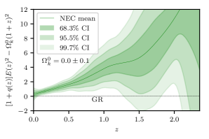
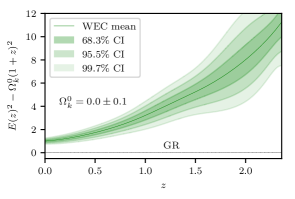
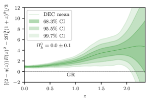
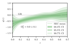
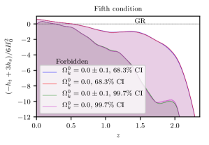
We first analyze the ECs in the context of GR. From Eqs. (22–26), we have that the ECs are fulfilled at any redshift value if they are equal or greater than zero. Note that WEC2 corresponds to the NEC in GR. Figures 1 and 2 show the MCMC results for the case where we consider a Gaussian prior on with zero mean and scatter 0.10. The green solid lines represent the ECs means and the shaded areas are the , and confidence intervals (CIs) at numerous redshift values in the range . The results for the other two cases, flat and , are pretty similar to this one. One must be careful when interpreting these plots. Note that each function value, e.g, , for a fixed value of has a posterior distribution. The plots show the mean and the , and areas around the mean. Furthermore, these values are obtained by marginalizing over all other function values and nuisance parameters (). Consequently, Figs. 1 – 5 do not show the correlations between different redshifts and must be interpreted accordingly.
The WEC (Eq. (24), left-lower panel of Fig. 1) is fulfilled in the entire redshift interval, and the DEC (right-lower panel) presents a violation within CI just for roughly in the three study cases, which is a highly degenerated region due to the few number of data points.
In turn, the upper panel of Fig. 1 shows that NEC is violated within CI for , and , where the last is in the degenerated region of the [and ] reconstruction. We note that these violation intervals are narrower than those obtained in Refs. Lima et al. (2008a, b) using only SNe Ia data and , where the violations were present for and . Despite of using a larger SNe Ia sample and BAO and data, it is worth mentioning that the reconstruction method used in the present work is less restrictive than that in Lima et al. (2008a, b),222The current reconstruction is based on cubic splines, whereas Lima et al. (2008a, b) used linear splines. and it was calibrated such that the bias contributes only with of the total error budget. The NEC, WEC and DEC results obtained for the flat and cases are pretty similar to those presented in Fig. 1.
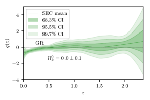
The most interesting result concerns SEC, since this is the only EC we expect to be violated, which is tightly linked with the recent accelerated expansion of the Universe. Figure 2 shows the reconstructed deceleration function, namely the mean curve along with the , and CIs. We note (left panel) that the evidence for SEC violation takes place over the entire redshift interval. In fact, we obtain SEC’s fulfillment within CI just for (for the other two cases, we have ). In VPL Vitenti and Penna-Lima (2015) this fulfillment was observed in the range . Despite the reconstruction methodology be the same used here, the differences result from some distinct and new BAO and data points (e.g., Moresco (2015); Ata et al. (2018); Bautista et al. (2017)) used in the analysis.
Contrarily to the new constraints for NEC, SEC violation is stronger than those obtained in previous work. The right panel of Fig. 2 highlights the redshift interval where we obtain the most restrictive constraints. For instance, SEC is violated with more than CI for for the three cases studied, whereas in VPL Vitenti and Penna-Lima (2015) this range was , and and in Refs. Lima et al. (2008a, b), respectively, using only SNe Ia data. In short, the most current SNe Ia, BAO and data strengthens the evidence of an accelerated expansion of the Universe. For instance, calculating the posterior for for we found that for all points in our sample of the posterior. This means that the probability of finding is smaller than (one in the number of posterior sampled points), which translates to at least confidence level.

As shown above, the fulfillment/violation of the ECs in the GR case can be directly tested since the bounds need just to be compared to constant values (dashed lines in Figs. 1 and 2). Regarding the class of ETGs considered in this work, this is just valid for NEC and SEC as they have the same form in GR as in these ETGs and, therefore, the results and analyses presented above (upper panel of Figs. 1 and 2) are also valid for these ETGs. This is to be expected, since these conditions were obtained from the convergence conditions imposed directly on and our reconstruction method output is exactly .
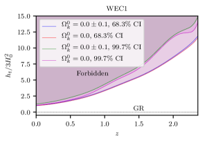
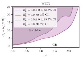
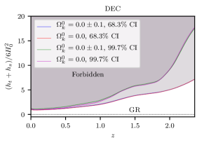
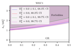
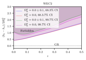
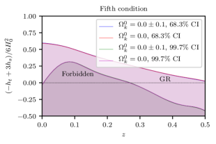
On the other hand, the remaining ECs, i.e., WEC1, WEC2 and DEC (Eqs. (24), (25) and (26), respectively), and also the FEC [Eq. (28)] involve not only , and , but also the arbitrary functions and of the modified gravity tensor . Consequently, instead of checking whether a condition is satisfied or not, our methodology allows one to put constraints on these functions [and their combinations, say ].
From the reconstructed and curves, we obtain now the observational constraints on the functions by requiring that WEC1, WEC2, DEC and FEC are fulfilled (see Eqs. (24), (25), (26) and (28)). Figure 3 shows the and CIs of the observational bounds obtained for the flat and cases. Note that WEC1 (left upper panel), WEC2 (right upper) and DEC (left lower) provide upper bounds on their respective functions whereas the FEC (right lower panel) gives a lower bound. The shaded areas in all four panels of Figure 3 indicate the values per redshift for which the respective conditions are violated. These forbidden areas are wider, i.e., more restrictive as the redshift values decrease due to the larger number of data points. Figure 4 shows the same results for the better constrained region . We see that the GR thresholds, which correspond to the case where , i.e., , of WEC1, WEC2, and DEC are fulfilled in the entire redshift interval. On the other hand, a quite different situation is verified for the FEC. The right lower panel of Fig. 4 shows that this condition is violated in GR theory within for . Since for GR the FEC is equivalent to SEC, the present result is consistent with that discussed previously (Fig. 2), where SEC violation in GR indicates that the Universe presents an accelerated expansion, which must be driven by a cosmological constant or an exotic fluid with equation of state, for example, of the type , with .
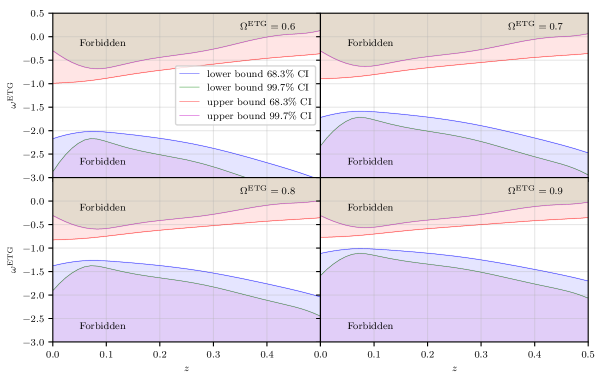
To go further without choosing a specific ETG, we need to make some assumptions about and . For this it is useful to use the language of an effective fluid. First we define and . Rewriting DEC and FEC using these variables, we can impose upper and lower bounds on , i.e.,
| (40) | ||||
| (41) |
where and . If the DE was explained by a dark fluid instead of an ETG, the same bounds above would be obtained. Nonetheless, in this case the FEC requires again that all fluids but the DE fluid satisfy the SEC. In addition, the upper bound (derived from DEC) requires a similar assumption, all fluids but the DE one must satisfy the DEC. It is interesting to note that the last mentioned condition is not necessary in the ETG case since, by definition, DEC already imposes conditions only on the ordinary matter.
Assuming that , we divide the bounds above by to obtain bounds on . In Fig. 5 we plot these bounds considering constant. Even though we do not expect, a priori, that is constant, these bounds plotted with different values of show approximately the bounds one would obtain if smoothly evolved inside the chosen redshift values. This amounts to show how these bounds can impose constraints on the behavior of the ETG. For instance, in Fig. 5 we note that the lower the value, the higher the evidence to obtain a phantom-like behavior. Naturally, the value of today must be closer to the one estimated by current data (Ref. Collaboration et al. (2016), for example, gives ). Nevertheless, for the evolution of can take it to different values depending on the specific dynamic of the ETG and, therefore, these bounds show the restrictions depending on how this function evolves in time.
5 Conclusion
Numerous propositions of modified gravity theories and also of the DE equation of state in the context of GR have been introduced and discussed in the last two decades to explain the recent accelerated expansion of the Universe. Therefore, one major task in cosmology is to constrain these models and also scrutinize their viability using observational data.
In this work we introduced a methodology to obtain observational bounds on a class of ETGs and also on the parameter space of a specific theory. This approach consists in requiring the fulfillment of the ECs, from which we obtain the theoretical bounds for the ETGs’ functions and/or paramaters.
We derived the ECs for ETGs for which matter is minimally coupled to geometry. Then, assuming a homogeneous and isotropic metric, we wrote these ECs in terms of the functions and , and the parameter . We also considered a fifth condition (called, for simplicity, FEC) stating that in the context of ETG there is no need to add fluids, other than the ordinary and dark matter, to explain the accelerated expansion of the Universe. Using the VPL model-independent reconstruction method Vitenti and Penna-Lima (2015) and SNe Ia, BAO, H(z) data, we obtained observational bounds on combinations of and as given in Eqs. (24), (25), (26) and (28).
We first studied the ECs in GR. We verified that WEC and DEC are fulfilled in the redshift interval . NEC is violated at very low redshifts (and also at higher values where the variance of the estimated curve is big, see Sect. 4). It is worth emphasizing that NEC violation is weaker than those obtained in Lima et al. (2008a, b). On the other hand, the evidence of SEC violation obtained in the present work is stronger than the previous ones Lima et al. (2008a, b); Vitenti and Penna-Lima (2015). In particular, there is an indication bigger than CI of the recent accelerated expansion of the Universe.
We also obtained the allowed/forbidden values for the WEC1, WEC2, DEC and FEC functions of and , as showed in Figs.3 and 4. Particularly, we have that GR violates the FEC within CI for which is equivalent to the violation of SEC. This reinforces our main idea that if the FEC if not fulfilled, than the theory requires the introduction of a DE fluid to explain the accelerated expansion of the Universe.
Notice that the present study considered a general class of ETGs and, therefore, we just obtained lower and upper bounds for different functions of and . However, applying this approach for a specific model, one will be able to obtain upper and lower bounds for a given function or parameters.
At last, in this regard we provided an example of possible results. By assuming a positive , we obtained bounds on the effective ETG equation of state as shown in Fig. 5. This proves to be potentially useful to determine the behavior of the ETG in the reconstructed redshift interval, from a phantom like behavior, , or the opposite direction, , depending on how evolves in time. Therefore, we consider that this method is a useful tool to constrain the parameter spaces of different ETGs. For instance, in Ref. Alves et al. (2017) we considered an ETG whose modified gravity term, i.e., the tensor , acts as a cosmological constant. In this context, we also studied two bimetric massive gravity theories putting constraints on their parameter space.
ACKNOWLEDGMENTS
MPL thanks the financial support from Labex ENIGMASS. SDPV acknowledges the support from BELSPO non-EU postdoctoral fellowship. MESA and JCNA would like to thank the Brazilian agency FAPESP for financial support under the thematic project # 2013/26258-4. JCNA thanks also the Brazilian agency CNPq (Grant No. 307217/2016-7) for the financial support. FCC was supported by CNPq/FAPERN/PRONEM. This research was performed using the Mesu-UV supercomputer of the Pierre & Marie Curie University | France (UPMC) and the computer cluster of the State University of the Rio Grande do Norte (UERN) | Brazil. This study was financed in part by the Coordenação de Aperfeiçoamento de Pessoal de Nível Superior - Brasil (CAPES) - Finance Code 001.
References
- Schuecker et al. (2003) P. Schuecker, R. R. Caldwell, H. Böhringer, C. A. Collins, L. Guzzo, and N. N. Weinberg, Astron. Astrophys. 402, 53 (2003), astro-ph/0211480.
- Santos et al. (2006) J. Santos, J. S. Alcaniz, and M. J. Rebouças, Phys. Rev. D 74, 067301 (2006), astro-ph/0608031.
- Gong and Wang (2007) Y. Gong and A. Wang, Phys. Lett. B 652, 63 (2007), 0705.0996.
- Santos et al. (2007a) J. Santos, J. S. Alcaniz, N. Pires, and M. J. Rebouças, Phys. Rev. D 75, 083523 (2007a), astro-ph/0702728.
- Lima et al. (2008a) M. P. Lima, S. Vitenti, and M. J. Rebouças, Phys. Rev. D 77, 083518 (2008a), 0802.0706.
- Lima et al. (2008b) M. P. Lima, S. D. P. Vitenti, and M. J. Rebouças, Phys. Lett. B 668, 83 (2008b), 0808.2467.
- Wald (1984) R. M. Wald, General Relativity (University of Chicago Press, Chicago, 1984).
- Capozziello and De Laurentis (2011) S. Capozziello and M. De Laurentis, Phys. Rept. 509, 167 (2011), 1108.6266.
- Nojiri and Odintsov (2011) S. Nojiri and S. D. Odintsov, Phys. Rep. 505, 59 (2011), 1011.0544.
- Capozziello et al. (2015) S. Capozziello, F. S. N. Lobo, and J. P. Mimoso, Phys. Rev. D 91 (2015).
- Santos et al. (2007b) J. Santos, J. S. Alcaniz, M. J. Rebouças, and F. C. Carvalho, Phys. Rev. D 76, 083513 (2007b), 0708.0411.
- Bertolami and Sequeira (2009) O. Bertolami and M. C. Sequeira, Phys. Rev. D 79 (2009).
- Wang et al. (2010) J. Wang, Y.-B. Wu, Y.-X. Guo, W.-Q. Yang, and L. Wang, Phys. Lett. B 689, 133 (2010).
- Wang and Liao (2012) J. Wang and K. Liao, Class. Quantum Grav. 29, 215016 (2012).
- Santos et al. (2017) C. S. Santos, J. Santos, S. Capozziello, and J. S. Alcaniz, Gen. Rel. Gravit. 49, 50 (2017), 1606.02212v4.
- Atazadeh et al. (2009) K. Atazadeh, A. Khaleghi, H. R. Sepangi, and Y. Tavakoli, Int. J. Mod. Phys. D18, 1101 (2009), 0811.4269.
- García et al. (2011) N. M. García, T. Harko, F. S. N. Lobo, and J. P. Mimoso, Phys. Rev. D 83 (2011).
- Banijamali et al. (2012) A. Banijamali, B. Fazlpour, and M. R. Setare, Astrophys. Space Sci. 338, 327 (2012), 1111.3878.
- Atazadeh and Darabi (2014) K. Atazadeh and F. Darabi, Gen Relativ Gravit 46 (2014).
- Alvarenga et al. (2013) F. G. Alvarenga, M. J. S. Houndjo, A. V. Monwanou, and J. B. C. Orou, Journal of Modern Physics 04, 130 (2013).
- Sharif and Zubair (2013) M. Sharif and M. Zubair, J. High Energy Phys. 12, 079 (2013), 1306.3450.
- Sharif et al. (2013) M. Sharif, S. Rani, and R. Myrzakulov, Eur. Phys. J. Plus 128 (2013).
- Azizi and Gorjizadeh (2017) T. Azizi and M. Gorjizadeh, EPL 117, 60003 (2017), 1701.00796.
- Sotiriou and Faraoni (2010) T. P. Sotiriou and V. Faraoni, Rev. Mod. Phys. 82, 451 (2010), 0805.1726.
- Vitenti and Penna-Lima (2015) S. D. P. Vitenti and M. Penna-Lima, J. Cosmol. Astropart. Phys. 9, 045 (2015), 1505.01883.
- Betoule et al. (2014) M. Betoule, R. Kessler, J. Guy, J. Mosher, D. Hardin, R. Biswas, P. Astier, P. El-Hage, M. Konig, S. Kuhlmann, et al., Astron. Astrophys. 568, A22 (2014), 1401.4064.
- Beutler et al. (2011) F. Beutler, C. Blake, M. Colless, D. H. Jones, L. Staveley-Smith, L. Campbell, Q. Parker, W. Saunders, and F. Watson, Mon. Not. R. Astron. Soc. 416, 3017 (2011), 1106.3366.
- Ross et al. (2015) A. J. Ross, L. Samushia, C. Howlett, W. J. Percival, A. Burden, and M. Manera, Mon. Not. R. Astron. Soc. 449, 835 (2015).
- Alam et al. (2017) S. Alam, M. Ata, S. Bailey, F. Beutler, D. Bizyaev, J. A. Blazek, A. S. Bolton, J. R. Brownstein, A. Burden, C.-H. Chuang, et al., Mon. Not. R. Astron. Soc. 470, 2617 (2017), 1607.03155.
- Bautista et al. (2017) J. E. Bautista, N. G. Busca, J. Guy, J. Rich, M. Blomqvist, H. du Mas des Bourboux, M. M. Pieri, A. Font-Ribera, S. Bailey, T. Delubac, et al., Astron. Astrophys. 603, A12 (2017), 1702.00176.
- Ata et al. (2018) M. Ata, F. Baumgarten, J. Bautista, F. Beutler, D. Bizyaev, M. R. Blanton, J. A. Blazek, A. S. Bolton, J. Brinkmann, J. R. Brownstein, et al., Mon. Not. Roy. Astron. Soc. 473, 4773 (2018), 1705.06373.
- Stern et al. (2010) D. Stern, R. Jimenez, L. Verde, M. Kamionkowski, and S. A. Stanford, J. Cosmol. Astropart. Phys. 2, 008 (2010), 0907.3149.
- Moresco et al. (2012) M. Moresco, A. Cimatti, R. Jimenez, L. Pozzetti, G. Zamorani, M. Bolzonella, J. Dunlop, F. Lamareille, M. Mignoli, H. Pearce, et al., J. Cosmol. Astropart. Phys. 8, 006 (2012), 1201.3609.
- Moresco (2015) M. Moresco, Mon. Not. Roy. Astron. Soc. 450, L16 (2015), 1503.01116v1.
- Riess et al. (2016) A. G. Riess, L. M. Macri, S. L. Hoffmann, D. Scolnic, S. Casertano, A. V. Filippenko, B. E. Tucker, M. J. Reid, D. O. Jones, J. M. Silverman, et al., Astrophys. J. 826, 56 (2016), 1604.01424v3.
- Felice and Tsujikawa (2010) A. D. Felice and S. Tsujikawa, Living Rev. Relativ. 13 (2010).
- Harko and Lobo (2014) T. Harko and F. S. N. Lobo, Galaxies (2014), 1407.2013v2.
- Alves et al. (2017) M. E. S. Alves, F. C. Carvalho, J. C. N. de Araujo, M. Penna-Lima, and S. D. P. Vitenti, European Physical Journal C 78, 710 (2018), 1711.07259.
- Carloni et al. (2009) S. Carloni, E. Elizalde, and S. Odintsov, Gen. Rel. Grav. (2009), 0907.3941v2.
- Capozziello et al. (2014) S. Capozziello, O. Farooq, O. Luongo, and B. Ratra, Phys. Rev. D 90, 044016 (2014), 1403.1421.
- Hawking and Ellis (1973) S. W. Hawking and G. F. R. Ellis, The large scale structure of space-time (Cambridge University Press, England, 1973).
- Riess et al. (1998) A. G. Riess, A. V. Filippenko, P. Challis, A. Clocchiattia, A. Diercks, P. M. Garnavich, R. L. Gilliland, C. J. Hogan, S. Jha, R. P. Kirshner, et al. (Supernova Search Team), Astron. J. 116, 1009 (1998), astro-ph/9805201.
- Perlmutter et al. (1999) S. Perlmutter, G. Aldering, G. Goldhaber, R. A. Knop, P. Nugent, P. G. Castro, S. Deustua, S. Fabbro, A. Goobar, D. E. Groom, et al. (Supernova Cosmology Project), Astrophys. J. 517, 565 (1999), astro-ph/9812133.
- Tegmark et al. (2006) M. Tegmark, D. J. Eisenstein, M. A. Strauss, D. H. Weinberg, M. R. Blanton, J. A. Frieman, M. Fukugita, J. E. Gunn, A. J. S. Hamilton, G. R. Knapp, et al., Phys. Rev. D 74, 123507 (2006), astro-ph/0608632.
- DES Collaboration et al. (2017) DES Collaboration, T. M. C. Abbott, F. B. Abdalla, A. Alarcon, J. Aleksić, S. Allam, S. Allen, A. Amara, J. Annis, J. Asorey, et al., ArXiv e-prints (2017), 1708.01530.
- Hinshaw et al. (2013) G. Hinshaw, D. Larson, E. Komatsu, D. N. Spergel, C. L. Bennett, J. Dunkley, M. R. Nolta, M. Halpern, R. S. Hill, N. Odegard, et al., Astrophys. J. Suppl. Ser. 208, 19 (2013), 1212.5226.
- Collaboration et al. (2016) P. Collaboration, P. A. R. Ade, N. Aghanim, M. Arnaud, M. Ashdown, J. Aumont, C. Baccigalupi, A. J. Banday, R. B. Barreiro, J. G. Bartlett, et al., Astron. Astrophys. (2016), 1502.01589v3.
- Turyshev (2008) S. G. Turyshev, Usp. Fiz. Nauk (2008), 0809.3730v2.
- Dias Pinto Vitenti and Penna-Lima (2014) S. Dias Pinto Vitenti and M. Penna-Lima, Astrophysics Source Code Library (2014), ascl:1408.013.
- Goodman and Weare (2010) J. Goodman and J. Weare, CAMCoS 5, 65 (2010).
- Doux et al. (2017) C. Doux, M. Penna-Lima, S. D. P. Vitenti, J. Tréguer, E. Aubourg, and K. Ganga, Mon Not R Astron Soc. 480, 5386-5411 (2018), 1706.04583.