Gapless Spin Excitations in the $S=1/2$ Kagome- and Triangular-Lattice Heisenberg Antiferromagnets

Abstract

The $S=1/2$ kagome- and triangular-lattice Heisenberg antiferromagnets are investigated using the numerical exact diagonalization and the finite-size scaling analysis. The behaviour of the field derivative at zero magnetization is examined for both systems. The present result indicates that the spin excitation is gapless for each system.

url]http://cmt.spring8.or.jp/

1 Introduction

Frustration in magnets is one of important topics in the field of the strongly correlated electron systems. Among such magnets, the kagome- and triangular-lattice antiferromagnets attract a lot of interests. Since discoveries of several candidate materials of the kagome-lattice antiferromanget; the herbertsmithite[1, 2], the volborthite[3, 4] and the vesignieite[5], particularly, the study on this system has been accelerated. The quantum spin-fluid behaviour of the system was predicted by many theoretical studies[6, 7, 8, 9, 10, 11, 12, 13, 14, 15, 16, 17, 18]. The $U(1)$ Dirac spin-liquid theory[13] indicated a gapless spin excitation in the thermodynamic limit, which has been supported by the recent variational approach[19, 20]. Our recent numerical diagonalization study[21] also concluded that the system is gapless. On the other hand, the recent density matrix renormalization group (DMRG) analyses[22, 23, 24] suggested that the system has a finite spin gap even in the thermodynamic limit and supported the $Z_{2}$ topological spin-liquid picture[6]. Thus whether the $S=1/2$ kagome-lattice antiferromagnet has a spin gap or not is still theoretically controversial, although the recent neutron scattering experiment of the single crystal of the herbertsmithite[25, 26] suggested that the system is gapless.

On the other hand, the triangular-lattice antiferromagnet is widely believed to be gapless, based on the previous precise numerical analysis[27]. Thus it would be interesting to compare the low-lying spin excitation of the kagome-lattice antiferromagnet with the one of the triangular lattice. In this paper, using the recently developed field-derivative analysis based on the numerical diagonalization of finite-size clusters[28], we try to approach the spin-gap issue of the $S=1/2$ kagome-lattice antiferromagnet, as well as the triangular-lattice one. When one examines field-derivatives of the magnetization within the numerical data for finite-size systems, it is difficult to eliminate finite-size effects completely. It is therefore required to reduce such effects by means of a feasible way. Under these circumstances, the purpose of this study is to present such a field-derivative analysis based on numerical data whose finite-size deviations are presumably reduced. The kagome- and triangular-lattice antiferromagnets have wide diversity of further studies in various aspects. Under large magnetic fields, nontrivial anomalous behaviours are observed in their magnetization curves; however, the behaviours are different between the kagome- and triangular-lattice antiferromagnets [29, 30, 31]. Such behaviors were also examined in various frustrated magnets[32, 33, 34, 35, 36]. A randomness effect in these systems was additionally examined[37, 38]. Under such circumstances, the present study tackles a fundamental issue concerning properties of systems without effects owing to significantly large fields and randomness are investigated.

2 Model and Calculation

Using the numerical exact diagonalization of finite-size clusters under periodic boundary condition, we investigate the $S=1/2$ kagome- and triangular-lattice Heisenberg antiferromagnets defined by the Hamiltonian

$${\cal H}=\sum_{\langle i,j\rangle}{\bf S}_{i}\cdot{\bf S}_{j},$$ (1)

where site $i$ is assumed to be the vertices of the kagome or triangular lattice. Here, $\langle i,j\rangle$ runs over all the nearest-neighbor pairs on each lattice. For an $N$-site system, we consider subspaces characterized by $M=\sum_{j}S_{j}^{z}$; we obtain the lowest energy denoted by $E(N,M)$ of the Hamiltonian matrix in each subspace. We calculate all the values of $E(N,M)$ available for the clusters up to $N=$36 by the numerical diagonalization. The diagonalization is carried out based on the Lanczos algorithm and/or the Householder algorithm. Part of the Lanczos diagonalizations were carried out using an MPI-parallelized code which was originally developed in the study of Haldane gaps[39]. The usefulness of our program was confirmed in large-scale parallelized calculations[21, 31, 40, 41, 42].

3 Field-derivative analysis

In order to investigate the low-lying spin excitation, we apply the field-derivative analysis which was developed in our previous work[28]. The argument of the analysis is briefly reviewed as follows: the effect of the applied external magnetic field $h$ is described by the Zeeman energy term

$${\cal H}_{Z}=-h\sum_{j}S_{j}^{z}.$$ (2)

The energy of ${\cal H}$ per site in the thermodynamic limit is defined as

$${{E(N,M)}\over N}\sim\epsilon(m)\qquad(N\rightarrow\infty),$$ (3)

where $m=M/(SN)$ is the magnetization normalized by the saturated magnetization $SN$. If we assume $\epsilon(m)$ is an analytic function of $m$, the spin excitation energy would become

$$E(N,M+1)-E(N,M)\sim\frac{1}{S}\left(\epsilon^{\prime}(m)+\frac{1}{2}\epsilon^{\prime\prime}(m){1\over NS}+\cdots\right).$$ (4)

Thus, this equation gives the quantity corresponding to the width of the magnetization plateau at $m$ as follows,

$$(E(N,M+1)-E(N,M))-(E(N,M)-E(N,M-1))\sim\epsilon^{\prime\prime}(m)\frac{1}{NS^{2}}.$$ (5)

Minimizing the energy of the total Hamiltonian ${\cal H}+{\cal H}_{Z}$, the ground state magnetization curve is derived by

$$h=\epsilon^{\prime}(m)/S.$$ (6)

The field derivative of the magnetization is defined as

$$\chi\equiv{{dm}\over{dh}}={S\over{\epsilon^{\prime\prime}(m)}}.$$ (7)

If we assume $\chi\not=0$, namely $\epsilon^{\prime\prime}(m)$ is finite, the magnetization plateau at $m$ would vanish in the thermodynamic limit, because of (5). Thus a necessary condition for the existence of a magnetization plateau at $m$ is $\chi=0$ in the thermodynamic limit. Now we apply this argument for the spin gap. We should examine the case of $h\rightarrow 0$ corresponding to $m=0$. In this case, the equation (5) can be rewritten as

$$2\Delta_{N}\sim\epsilon^{\prime\prime}(0)\frac{1}{NS^{2}},$$ (8)

where $\Delta_{N}=E(N,1)-E(N,0)$ is the spin gap for an $N$-spin cluster. Thus a necessary condition of the finite spin gap would be $\chi=0$ at $m=0$ in the thermodynamic limit.

In order to estimate $\chi$ at $m=0$ from discrete data for finite-size systems, it is the most simple way to use neighboring three data in the form $\chi_{3}$ defined as

$$\chi_{3}^{-1}=NS[-2E(N,M)+E(N,M+1)+E(N,M-1)].$$ (9)

Actually, eq. (9) was used in our previous examination[28]. However, a significant possibility cannot be denied that there remain deviations from the ideal quantity owing to the discreteness. It is expected to reduce the deviations if one uses neighboring five data instead of the above three under the assumption that $\epsilon(m)$ is analytic. In the method employing neighboring five data, we use $\chi_{5}$ defined as

$$\chi_{5}^{-1}= NS \left[-\frac{5}{2}E(N,M)+\frac{4}{3}(E(N,M+1)+E(N,M-1))\right.$$ (10)

$$\left.-\frac{1}{12}\left(E(N,M+2)+E(N,M-2)\right)\right].$$

In the thermodynamic limit, $\chi_{3}$ should agree with $\chi_{5}$. We show the estimated $\chi_{3}$ and $\chi_{5}$ for the kagome- and triangular-lattice antiferromagnets in the following sections.

4 Kagome-lattice antiferromagnet

We investigate the field derivative of the magnetization $\chi$ for the $S=1/2$ kagome-lattice antiferromagnet.

Let us, first, show differences between $\chi_{3}$ obtained from eq. (9) and $\chi_{5}$ obtained from eq. (10); results are depicted in Fig. 1. One can confirm that the differences are small irrespective of the values of $m$. The smallness is also observed irrespective of $N$. It is expected that we can obtain better estimates of $\chi$ by the small deviations from $\chi_{3}$ to $\chi_{5}$.

Let us, next, focus our attention on the system-size dependence of the field derivative of the magnetization at $m=0$. We plot $\chi_{5}$ at $m=0$ calculated by the form (10) as a function of $1/N$ for $N$=36, 30, 24, 18, and 12 in Figure 2. Although the system-size dependence exhibits a slight oscillation, the dependence of our data is quite small. Our plotted data seem to go to an nonzero value for $N\rightarrow\infty$. The nonzero extrapolated value suggests that the spin excitation of kagome-lattice antiferromagnet is gapless in the thermodynamic limit.

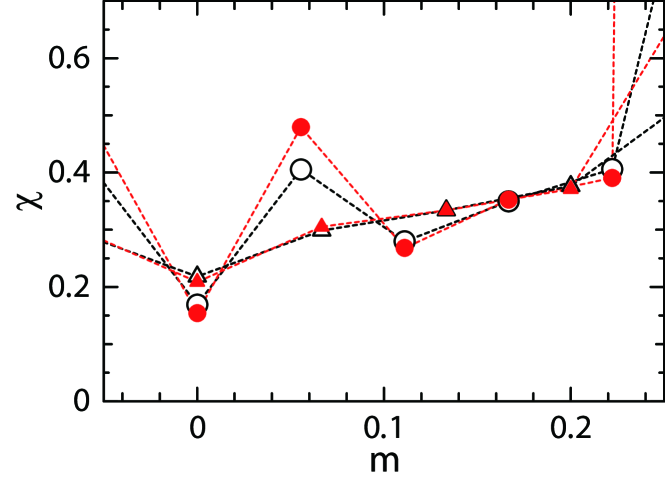
Figure 1: Field-derivative of the magnetization as a function of $m$ for $N=36$ and 30 in the kagome-lattice antiferromagnet. Circles and triangles denote results for $N=36$ and 30, respectively. Black open and red closed symbols represent results of $\chi_{3}$ obtained from eq. (9) and $\chi_{5}$ obtained from eq. (10), respectively.

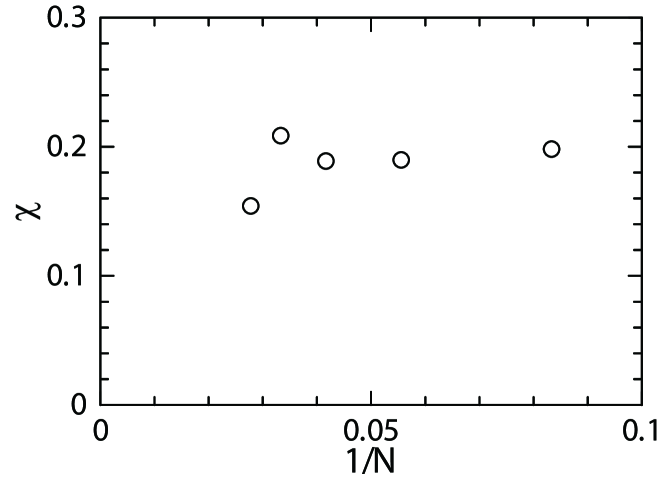
Figure 2: The system-size dependence of the field derivative of the magnetization at $m=0$ estimated by the form (10) in the case of the kagome-lattice antiferromagnet. Numerical data are plotted as a function of $1/N$ for $N$=36, 30, 24, 18, and 12.

5 Triangular-lattice antiferromagnet

In order to confirm the validity of the present method, we apply it for the $S=1/2$ triangular-lattice antiferromagnet, for which the triplet excitation is gapless.

Figure 3 presents differences between $\chi_{3}$ obtained from eq. (9) and $\chi_{5}$ obtained from eq. (10); results are given for $N=36$ and 30. One can confirm that the differences are small irrespective of the values of $m$. The smallness is also observed irrespective of $N$. Note here that the differences are even smaller than in the case of the kagome-lattice antiferromagnet in Fig. 1.

Figure 4 provides us with the system-size dependence of the field derivative of the magnetization at $m=0$; $\chi_{5}$ at $m=0$ calculated by the form (10) are plotted as a function of $1/N$ for $N$=36, 30, 24, 18, and 12. The oscillating behaviour in the system-size dependence seems smaller than in the case of the kagome-lattice antiferromagnet. The result of the dependence indicates that the system has a non-zero field derivative at $m=0$ in the thermodynamic limit. The nonzero extrapolated value suggests that the spin excitation of triangular-lattice antiferromagnet is gapless, which is consistent with a widely believed consensus of the gapless feature of the triangular-lattice antiferromagnet. Thus it is confirmed that the present method is valid.

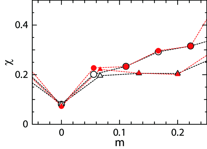
Figure 3: Field-derivative of the magnetization as a function of $m$ for $N=36$ and 30 in the triangular-lattice antiferromagnet. Circles and triangles denote results for $N=36$ and 30, respectively. Black open and red closed symbols represent results of $\chi_{3}$ obtained from eq. (9) and $\chi_{5}$ obtained from eq. (10), respectively.

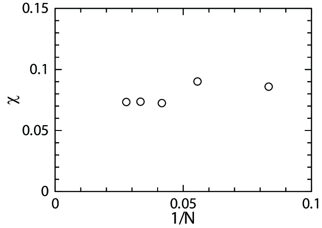
Figure 4: The system-size dependence of the field derivative of the magnetization at $m=0$ estimated by the form (10) in the case of the triangular-lattice antiferromagnet. Numerical data are plotted as a function of $1/N$ for $N$=36, 30, 24, 18, and 12.

6 Summary

The low-lying spin excitations of the kagome- and triangular-lattice antiferromagnets are investigated using the numerical diagonalization up to $N=36$. The analysis of the field derivative of the magnetization $\chi$ is successfully applied to these two systems and we conclude that these systems are gapless in the spin excitation. Our numerical results strongly suggest that the gapless spin excitation in the kagome-lattice antiferromagnet, as well as the triangular-lattice one. The study presents an analysis based on numerical data whose finite-size effects are expected to be reduced because $\chi$ is estimated from the neighboring five data of the ground-state energies. The present method would be applicable for various frustrated quantum spin systems.

References

- [1] M. P. Shores, E. A. Nytko, B. M. Barlett, and D. G. Nocera, J. Am. Chem. Soc. 127, 13462 (2005).
- [2] P. Mendels and F. Bert, J. Phys. Soc. Jpn. 79, 011001 (2010).
- [3] H. Yoshida, Y. Okamoto, T. Tayama, T.Sakakibara, M.Tokunaga, A. Matsuo, Y. Narumi, K. Kindo, M. Yoshida, M. Takigawa, and Z. Hiroi, J. Phys. Soc. Jpn. 78, 043704 (2009).
- [4] M. Yoshida, M. Takigawa, H. Yoshida, Y. Okamoto, and Z. Hiroi, Phys. Phys. Lett. 103, 077207 (2009).
- [5] Y. Okamoto, H. Yoshida, and Z. Hiroi, J. Phys. Soc. Jpn. 78, 033701 (2009).
- [6] S. Sachdev, Phys. Rev. B 45, 12377 (1992).
- [7] T. Nakamura and S. Miyashita, Phys. Rev. B 52, 9174 (1995).
- [8] P. Lecheminant, B. Bernu, C. Lhuillier, L. Pierre, and P. Sindzingre, Phys. Rev. B 56, 2521 (1997).
- [9] Ch. Waldtmann, H.-U. Everts, B. Bernu, C. Lhuillier, P. Sindzingre, P. Lecheminant and L. Pierre, Eur. Phys. J. B 2, 501 (1998).
- [10] F. Mila, Phys. Rev. Lett. 81, 2356 (1998).
- [11] M. Hermele, T. Senthil and M. P. A. Fisher, Phys. Rev. B 72, 104404 (2005).
- [12] R. R. P. Singh and D. A. Huse, Phys. Rev. B 76, 180407(R) (2007).
- [13] Y. Ran, M. Hermele, P. A. Lee and X. -G. Wen, Phys. Rev. Lett. 98, 117205 (2007).
- [14] H. C. Jiang, Z. Y. Weng and D. N. Sheng, Phys. Rev. Lett. 98, 117203 (2008).
- [15] O. Cepas, C. M. Fong, P. W. Leung, and C. Lhuillier, Phys. Rev. B 78, 140405(R) (2008).
- [16] P. Sindzingre and C. Lhuillier, Europhys. Lett. 88, 27009 (2009).
- [17] G. Evenbly and G. Vidal, Phys. Rev. Lett. 104, 187203 (2010).
- [18] S. Capponi, O. Derzhko, A. Honecker, A. M. Läuchli and J. Richter, Phys. Rev. B 88, 144416 (2013).
- [19] Y. Iqbal, D. Poilblanc and F. Becca, Phys. Rev. B 89, 020407(R) (2014).
- [20] Y. Iqbal, D. Poilblanc and F. Becca, Phys. Rev. B 91, 020402(R) (2015).
- [21] H. Nakano and T. Sakai, J. Phys. Soc. Jpn. 80, 053704 (2011).
- [22] S. Yan, D. A. Huse and S. R. White, Science 332, 1173 (2011).
- [23] S. Depenbrock, I. P. McCulloch and U. Schollwöck, Phys. Rev. Lett. 109, 067201 (2012).
- [24] S. Nishimoto, N. Shibata and C. Hotta, Nat. Commun. 4, 2287 (2013).
- [25] T. Han et al., Nature Commun. 492, 406 (2012).
- [26] T. Han et al., Phys. Rev. Lett. 108, 157202 (2012).
- [27] B. Bernu, P. Lecheminant, C. Lhuillier and L. Pierre, Phys. Rev. B 50, 10048 (1994).
- [28] T. Sakai and H. Nakano, Polyhedron 126, 42 (2017).
- [29] H. Nakano and T. Sakai, J. Phys. Soc. Jpn. 79, 053707 (2010).
- [30] T. Sakai and H. Nakano, Phys. Rev. B 83, 100405(R) (2011).
- [31] H. Nakano and T. Sakai, J. Phys. Soc. Jpn. 83, 104710 (2014).
- [32] H. Nakano and T. Sakai, J. Phys. Soc. Jpn. 82, 083709 (2013).
- [33] H. Nakano, Y. Hasegawa, and T. Sakai, J. Phys. Soc. Jpn. 83, 084709 (2014).
- [34] H. Nakano, M. Isoda, and T. Sakai, J. Phys. Soc. Jpn. 83, 053702 (2014).
- [35] M. Isoda, H. Nakano, and T. Sakai, J. Phys. Soc. Jpn. 83, 084710 (2014).
- [36] H. Nakano and T. Sakai, J. Phys. Soc. Jpn. 86, 063702 (2017).
- [37] K. Watanabe, H. Kawamura, H. Nakano, and T. Sakai, J. Phys. Soc. Jpn. 83, 034714 (2014)
- [38] T. Shimokawa, K. Watanabe, and H. Kawamura, Phys. Rev. B 92, 134407 (2015).
- [39] H. Nakano and A. Terai, J. Phys. Soc. Jpn. 78, 014003 (2009).
- [40] H. Nakano, S. Todo, and T. Sakai, J. Phys. Soc. Jpn. 82, 043715 (2013).
- [41] H. Nakano and T. Sakai, J. Phys. Soc. Jpn. 84, 063705 (2015).
- [42] H. Nakano, Y. Hasegawa, and T. Sakai, J. Phys. Soc. Jpn. 84, 114703 (2015).