Neural Network Forecast of the Sunspot Butterfly Diagram



1 Introduction

introduction The sunspots are mostly a visible phenomenon in the solar photosphere and a manifestation of solar activity. One can find extensive bibliography about the solar cycle, its causes and consequences. Here we emphasise just a few number of previous results and further detail can be obtained in the recent reviews (Hathaway, 2015a, b) and references therein. Since Hale (1908), it is known that sunspots contain strong magnetic fields. These decrease the energy flux considerably and so the sunspots appear darker than the surroundings.

We know, since Schwabe (1844), that the rise of the sunspots in the solar surface is cyclic but not periodic, with erratic time lapses between maxima and/or minima that can span between 9 to 13 years. However, one can establish an average period time of about 11 years. Moreover, thanks to the analysis of the cosmogenic isotopes, e.g. ¹⁴C and ¹⁰Be (Beer, Tobias, and Weiss, 1998) it is possible to reconstruct the solar cycle back to more than $10,000\text{\,}\mathrm{y}$ears which is particularly interesting for paleoclimatology (Solanki et al., 2004). Recently, Luthardt and Rößler (2017) have shown some evidence that there is a cycle around 11 years on 300-million-year fossilised tree rings. This could mean that the sunspot cycle has been around for a much longer time scale than our current direct observation record.

Being weakly chaotic (Weiss, 1988, 1990; Mundt, Maguire, and Chase, 1991; Letellier et al., 2006; Spiegel, 2009; Arlt and Weiss, 2014) and one of the longest continuously recorded daily measurement made in science (Owens, 2013), the sunspot series is rightly considered as one of the top benchmarks for time series forecasting.

There is quite a large body of research on forecasting the sunspot time series, in particular the strength, the length and the maximum of the next cycle. However, as indicated by the analysis presented at the American Geophysical Union (AGU) 2008 meeting (Pesnell, 2008, 2012), there seems to exist more forecasts than possible future data scenarios, as shown in the “piano plot” introduced by William Dean Pesnell, in his summary of the literature for predictions of the current cycle maximum solar spot number. Depending on the most realistic maximum number of sunspots (Acero et al., 2017), one would think that there are more articles predicting the next cycle sunspot maximum than attainable physical possibilities. Pesnell’s plot emphasises that metrics such as the sunspot number may not contain enough information to decide among distinct forecasting methods.

It was under these motivations that one of us (Covas, 2017) attempted to use a model based on spatial-temporal embeddings to forecast the sunspot diagram, demonstrating how a pure mathematical model can be used to do a spatial-temporal forecast (latitude and time), based on the full dataset for the solar spot coverage area and its corresponding latitude, from 1874 up to 2015. That work, however, was not the first one to attempt to predict or reconstruct the entire sunspot diagram (space and time, not just time). Jiang et al. (2011) analysed the sunspot diagram in its entirety to calculate correlations between several quantities of sunspot groups against the cycle strength and phase. With these, they were then able to reasonably reconstruct the sunspot spatial-temporal pattern.

In this article, we propose an approach by forecasting the full spatial-temporal sunspot diagram, using exactly the same data as in Covas (2017), by means of neural network techniques. A very large number of authors (from the early 1990’s up to now) have already attempted to use neural networks to forecast pure temporal aspects of the sunspot cycle (Pesnell, 2012, 2016, see references in these reviews). All of those authors, however, have limited themselves to forecasts in time only, not space and time. So, in contrast and as proposed, we attempt to forecast the full sunspot diagram, by means of neural networks. We believe that by including one further dimension to the usual one-dimensional forecasts in the literature, one should, in the future, be able to better decide between the multitude of forecasting methods.

The article is organised as follows. In Section method we introduce the method using neural networks for forecasts and give details of how to apply the approach to a dataset with one spatial and one temporal dimension. In Section results we apply the approach to the sunspot dataset. Finally, in Section conclusion we draw our conclusions and suggest future research ideas.

2 The Method: Feed-Forward Neural Networks

method

Here we propose an approach which is based on artificial neural networks (Lecun et al., 1998; Krizhevsky, Sutskever, and Hinton, 2017). We use a subset of neural networks called feed-forward artificial neural networks. These are basic networks that have an input layer, one or several hidden layers, and an output layer, fully connected but where no connection occurs backwards or on a loop. We train the network using the back-propagation algorithm (David E.; McClelland, 1989; Rumelhart, Hinton, and Williams, 1986) and we use on-line training (see Reed, 1999, and references therein) as recommended in the literature (Wilson and Martinez, 2003).

Most of the neural network literature on forecasting can be divided into two groups, one using time delays (Kim, Eykholt, and Salas, 1999) to construct the vector input patterns for the feed-forward neural network and another using what is called a recurrent network (Elman, 1990), where the information is allowed to cycle in a loop (Petrosian et al., 2000; Zhang and Xiao, 2000; Han et al., 2004; Zhang, 2009; Chandra and Zhang, 2012). Here we shall use only the former, mainly for simplicity, easiness of implementation, and interpretability. The time delay approach in the literature uses the embedding dimension and sometimes the derived time lags to create an appropriate set of input patterns (see, e.g. Cheng et al., 2014, and references therein). The extension to spatial-temporal forecasting follows the same approach, i.e. using lags and an embedding dimension, but in space and in time. The approach results from merging this technique with another forecasting method unrelated to neural networks and introduced in Parlitz and Merkwirth (2000) for the reconstruction of spatial-temporal datasets. In their article they used their approach successfully to both a spatial-temporal version of the Hénon map and to a synthetic dataset arising from evolving the Kuramoto-Sivashinsky non-linear model. Following on Parlitz and Merkwirth (2000), there was later an attempt to forecast financial spatial-temporal datasets by Covas and Mena (2011), with reasonable success, and also an attempt to use it for the sunspot diagram by Covas (2017). In those articles, a grid of inputs was built based on the two dimensional data series $s(n,m)$ to use in the search of the nearest neighbour in the embedding space, that once found, gave an approximation to the true future evolution in the original space. We shall describe this approach in Section Parlitz-Merkwirthmethod.

Although there is some limited research on the application of neural networks to spatial-temporal forecasting in several distinct settings (see, e.g. McDermott and Wikle, 2017; Pathak et al., 2018, 2017; Lu et al., 2017; Pathak et al., 2018; Raissi, Perdikaris, and Karniadakis, 2017b, a; Raissi, 2018; Raissi and Karniadakis, 2018, and references therein), we believe that this is the first time that neural networks have been applied in the specific context of sunspot spatial-temporal forecasting.

2.1 Input Layer Architecture

Parlitz-Merkwirthmethod

The input layer design we take can be seen as a spatial-temporal generalization of the time delay neural network method (Waibel et al., 1990; Luk, Ball, and Sharma, 2000; Frank, Davey, and Hunt, 2001; Oh, 2002; Sheng et al., 2003) together with a merge of the spatial-temporal method of Parlitz-Merwirth (Parlitz and Merkwirth, 2000), applied to feed-forward neural networks.

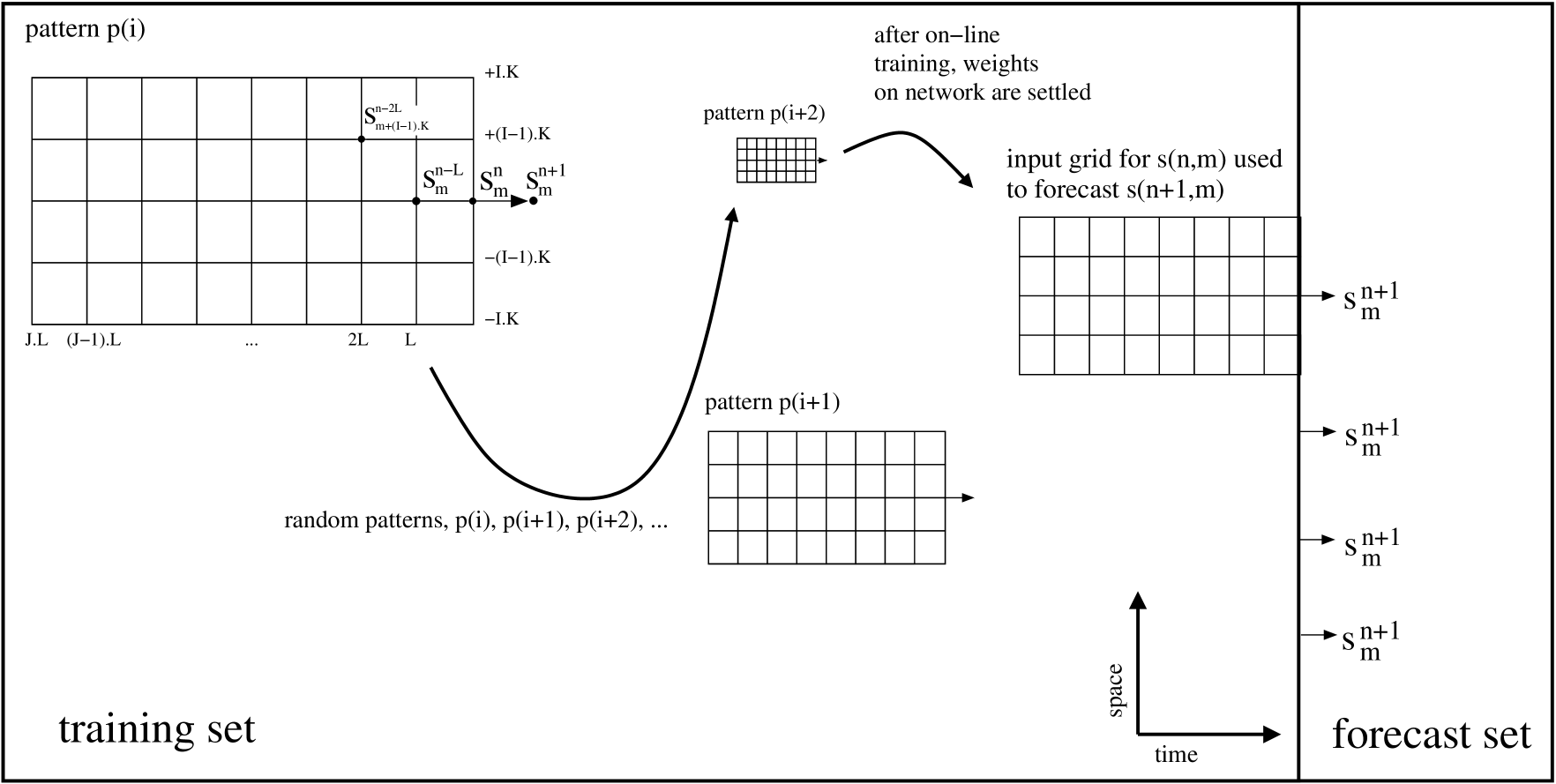
Figure 1.: Forecasting method illustration. One constructs an embedding space using delays, then assembles randomly positioned grid input patterns within the training set to pass to the neural network (in this figure we show 3 randomly selected input patterns). The input is a $(2I+1)(J+1)$ vector ${\bf x}(s^{n}_{m})$ and the target (output) to train the network is the value $s^{n+1}_{m}$. After training with a sequence of patterns $p(i),p(i+1),p(i+2),\ldots$ then the patterns adjacent to the forecast set are used to calculate the outputs to compare against the forecast. To forecast the $n+2$ slice we concatenate the previously predicted $n+1$ and progress accordingly.NeuralNetwork

The model is constructed using the concept of super-state vector ${\bf x}(s^{n}_{m})$ as described already in great detail (Covas, 2017) and we refer the reader to it for further reading. These super-state vectors have the following formula:

embedding$${\bf x}(s^{n}_{m})= \{ s^{n}_{m-IK},\ldots,s^{n}_{m},\ldots,s^{n}_{m+IK},$$

$$s^{n-L}_{m-IK},\ldots,s^{n-L}_{m},\ldots,s^{n-L}_{m+IK},\ldots$$

$$\ldots,s^{n-JL}_{m-IK},\ldots,s^{n-JL}_{m},\ldots,s^{n-JL}_{m+IK}\},$$

and are built from a rectangular grid of the original spatial-temporal data series ${\bf x}(s^{n}_{m})$. Again, as in Covas (2017), $I$ refers to the number of neighbours on each side in space, $J$ to the number of temporal ones, and $K$ is the spatial lag, while $L$, the final parameter, is the temporal lag. The $K$ and $L$ parameters, are chosen again as in Covas (2017). In that article the average mutual information method (Fraser and Swinney, 1986; Abarbanel and Gollub, 1996) was used to calculate the optimal spatial-temporal delays, and we use the same (we refer the reader to that article for further details). Regarding the embedding parameters $I$ and $J$, again we follow the approach as in Covas (2017) and use the false nearest neighbours algorithm (Kennel, Brown, and Abarbanel, 1992). These two approaches allow the feature selection architecture to be defined automatically before we attempt any neural network forecast.

These input vectors ${\bf x}(s^{n}_{m})$ (see Figure NeuralNetwork), are then passed as input to the neural network grid while the target (output) is $s^{n+1}_{m}$. Using this method, the number of input neurons is the same as the dimension of ${\bf x}(s^{n}_{m})$, i.e. $(2I+1)(J+1)$. It seems reasonable to define the input layer architecture in this way, and after extensive searches, we find that this architecture, with its four auto-calibrated parameters ($I$, $J$, $K$, $L$), seems to be optimal for forecasting. The number of output neurons needed for this approach is just one, i.e. the predicted $s^{n+1}_{m}$. Finally, the number of hidden nodes will be decided by trial and error later on, given that there seems to be no theoretically firm formula for the optimal number of these.

3 Results

results

3.1 The Dataset

The dataset used is available freely in Hathaway (2015a) and is exactly the same used in Covas (2017), in part to make sure we can do a comparison between the model presented here, i.e. a neural network forecast, against the model in Covas (2017), which was a non-linear embedding model. We refer the reader to that article for finer details of the dataset. To summarize here, the data is a latitude and time set of sunspot areas, covering 142 years. The base training set used the first 1646 temporal latitudinal values and the base test set is made of the remaining 242 time latitudinal values.

3.2 Neural Network Parameter Calibration

parameters

Given that we use exactly the same base dataset as in a previous article (Covas, 2017), we can use exactly the same calibration for the feature selection architecture parameters, i.e. $I$, $J$, $K$, $L$ in Equation embedding. The calibrated parameters for this base training set were $I=2$, $J=6$, $K=9$, and $L=70$, i.e.  each ${\bf x}(s^{n}_{m})$ is made of $(2I+1)(J+1)=2\times 2+1=5$ spatial neighbours by $6+1=7$ time delayed neighbours, with a spatial lag of $9$ latitudinal slices and a temporal lag or delay of $70$ Carrington rotations or time slices, corresponding to approximately 5.22 years. We shall use these choices of parameters to create training sets for the neural network and after the training, the input sets for the forecasts as depicted in Figure NeuralNetwork. Notice that this feature selection or feature representation choice, as done in Covas (2017), only depends on the training set, and therefore up to here, this approach is self-contained and auto-calibrated. However, other neural network parameters have to be decided empirically, as there is no agreed way to calculate them (see Stathakis, 2009, and references within). The most important is the number of hidden neurons on each hidden layer and the number of those layers. To keep the approach as simple as possible, we decided to use only one hidden layer. Regarding the number of hidden nodes $N_{h}$, there is again, as far as we know, no universally agreed procedure to decide what is the optimal number. Using too little will result in under-fitting, and too many in over-fitting, or worst, in fitting the noise of the input data patterns. In our case, we have calculated the optimal number of hidden nodes by trial and error, as our particular case study does not require large computational power (an entire run with one million iterations takes a few minutes to complete on an average personal computer). We have seen that the neural network can produce realistic results when the number of nodes is between 50 and 100 or so, with an optimal value of $N_{h}=70$ nodes. We shall use this value hereafter. We note that there are some algorithms, namely “pruning” and “constructive algorithms” (Cun, Denker, and Solla, 1990; Hassibi, Stork, and Wolff, ; Reed, 1999) that try to overcome this problem, by starting with a large network and calculating which of the weights or links on the network are superfluous. For the purpose of this article, given that the dataset is small, we will keep it as simple as possible and stay away from pruning and heuristic approaches and just do an exhaustive search. As for the back-propagation hyper-parameters, $\eta$ and $\alpha$, representing respectively the rate of learning and momentum of the algorithm, we shall use, based on our searches, the values of $\eta=0.3$ and $\alpha=0.01$. Notice that we use a variation of the algorithm with an adaptive learning rate $\eta_{n}=\nicefrac{{\eta}}{{\left(1+n/10000\right)}}$, where $\eta_{n}$ is the learning rate used at time step $n$. In addition to the depth and width of the hidden layer(s) architecture, another important degree of freedom is the choice of the activation function. Here for simplicity, we shall use the logistic or sigmoid function $\nicefrac{{1}}{{\left(1+e^{-x}\right)}}$ as the activation function for all layers. Another parametrization is what normalization to take (Reed, 1999). In the case of the sunspots, we have area values from a minimum of 0 to a maximum of $2580\text{\,}\mathrm{i}$n units of millionths of a hemisphere. One approach is to subtract the mean and divide by the standard deviation. However, the sunspot area distribution function does not follow a Gaussian distribution. In fact, the distribution is closer to a power law with an exponential cut-off, similar to the probability distribution function of the so called in-out intermittency (Ashwin, Covas, and Tavakol, 1999). So, we take another approach, namely to apply the transformation:

$$x\to\alpha_{nor}+\frac{\ln(1+x)}{\beta_{nor}},$$

where $\alpha_{nor}$ and $\beta_{nor}$ are the arbitrary shift and scaling constants, respectively. Again, there is no clear rule on how to choose these and we calibrate them by trial and error. We have seen that the neural network can produce realistic results when the $\alpha_{nor}=0$ and $\beta_{nor}=10$. We shall use these values hereafter. Our final free set of parameters relates to the initialization of the weights. We choose random numbers with a constant distribution between $[0,1]$ and shifted by $\alpha_{rng}$ and scaled by $\beta_{rng}$. We find that we obtain good results (as measured by the similarity index introduced below) around $\alpha_{rng}=-0.5$ and $\beta_{rng}=0.01$. We notice that for all parameters above, we conducted extensive stress testing and chose the parameters values above mentioned for which the similarity between the spatial-temporal forecast and the original real data was maximal.

3.3 Training and Forecast

originalforecast

To train the neural network, we have used one million iterations of different input patterns. Notice that the maximum number of different input patterns is $1646\times 50=$ $82,300\text{\,}\mathrm{p}$atterns. However, for neural network training, one randomly chooses patterns to optimize the weights, even if the number of iterations exceeds the number of unique patterns, and using this approach is equivalent to a stochastic progress towards the minima of the error function (Reed, 1999).

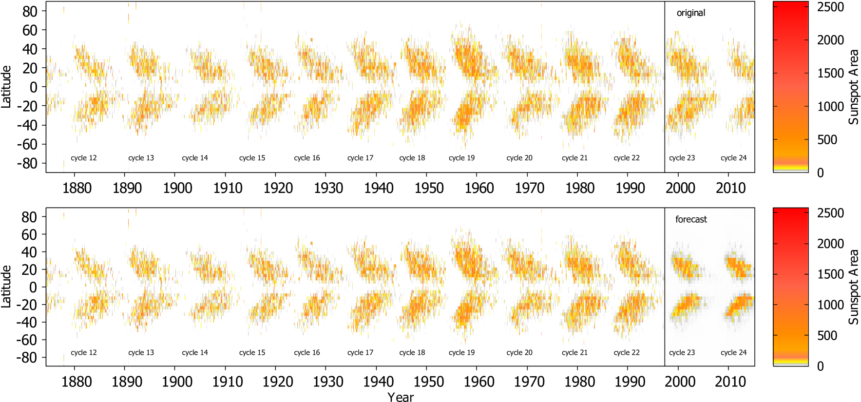
Figure 2.: Forecast of the last two sunspot solar cycles using spatial-temporal neural networks. We have used the parameters $I=2$, $J=6$, $K=9$, and $L=70$ (as in Covas, 2017). This figure is very similar to Figure 6 in that article, using exactly the same original dataset, but while Covas (2017) used a non-linear embedding method, we used the neural network method for the forecast. The fact that both methods result in similar forecasts and corresponding figures is reassuring, as it reinforces the adequacy of the feature selection approach based on non-linear embeddings. The specific neural network hyper-parameters used were: $\eta=0.3$, $\alpha=0.01$, $\alpha_{nor}=0$, $\beta_{nor}=10$, $\alpha_{rng}=-0.5$, $\beta_{rng}=0.01$, $N_{h}=70$ hidden nodes, run with one million pattern iterations, and the logistic or sigmoid function as the activation functions on both the hidden and output layer. The upper panel represents the sunspot dataset, divided into the base training set and the base test set. The lower panel represents the training together with the respective forecast. On both panels the split between training set and observed future dataset or forecast set is shown with a black line. Notice that, as in Covas (2017), the main characteristics of the sunspot diagram are reproduced, namely the overall intensity of the cycle and the sunspot band progress towards the equator are both present. Overall, the forecast is quite good from the qualitative point of view.Spatiotemporal_Forecasting_Sunspots_LastCycle

Using the best parameter calibrations from Section parameters, we can then proceed to forecast the base test set (made of Cycle 23 and the beginning of Cycle 24). We choose to split the full dataset into a training set consisting of data up and including Cycle 22 inclusive, with the remaining data being the forecast set. We choose this split partly because we want to forecast at least one entire cycle, and partly because we want to do a consistent comparison with the previous results in Covas (2017). The model outputs one latitudinal vector at a time, and we then stack that vector to the training set, and reuse the same calibrated parameters to forecast the next latitudinal vector. The results of this forecasting are depicted in Figure Spatiotemporal_Forecasting_Sunspots_LastCycle. The results show that this method can reproduce the two main features of the sunspot spatial-temporal original series, i.e. the amplitude shape of the cycle (resembling a butterfly wing, hence the usual name given to the sunspot cycle) and the sunspot band or wing progresses or moves towards the equator, although there are some quantitative differences, e.g. there seems to be a concentration of points on the forecast and the butterfly wings look denser. To strengthen this conclusion, we also depicted in Figure SolarForecastingNeuralNetworksSumOverLatitude the calculation of the total sunspot area (summed over latitudes) for the forecast and compared it with the observed one. It shows the total sunspot area time series, from both the original training set and the forecast set, and even if both sets are noisy, it demonstrates that the neural network approach can work not only in space and time but also on one-dimensional reductions like the latitudinal sum. This result seems to indicate that the neural network method is reasonably good at forecasting the first cycle but struggles when forecasting ahead to the next cycle. This is however not surprising, as usually the solar sunspot series is recognized as a seminal case of low dimensional chaos. It implies that there is a temporal limit for any reasonable predictability.

Further to the temporal average, we can also calculate the sum over time, to show the average sunspot area as a function of latitude, another aggregated metric. This is shown in Figure SolarForecastingNeuralNetworksSumOverTime and demonstrates that the method seems to be able to reproduce the real features in latitude as well as in time.

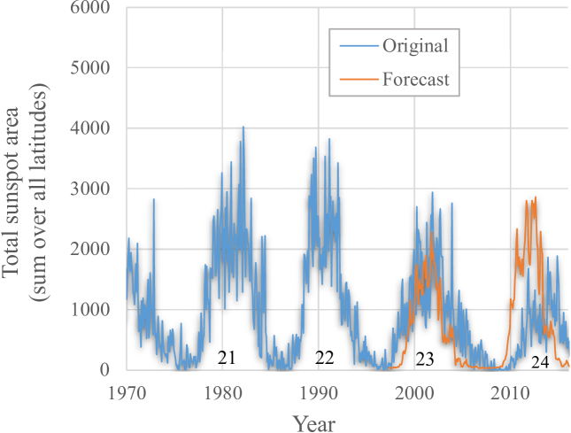
Figure 3.: Latitudinal sum of the sunspot area $A(t)$ and the forecast for the two last Cycles (23 and 24) - same scenario as in Figure Spatiotemporal_Forecasting_Sunspots_LastCycle. We have marked the cycle numbers near the horizontal axis. The forecast for Cycle 23 is reasonable but the method fails badly for Cycle 24, showing clearly the limitations of the approach at least in its current format.SolarForecastingNeuralNetworksSumOverLatitude

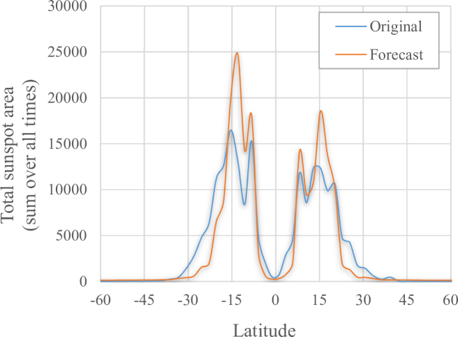
Figure 4.: Temporal sum of sunspot area $A(\theta)$ and the forecast for the two last cycles - same scenario as in Figure Spatiotemporal_Forecasting_Sunspots_LastCycle. The forecast gives a very similar latitudinal profile, with the two sunspot bands at mid-latitudes shown clearly on the plot.SolarForecastingNeuralNetworksSumOverTime

3.4 Structural Similarity

ssim

The novelty of the sunspot butterfly diagram forecasting approach presented here is that it attempts to predict in both space and time using neural networks. The question is, how does one verify that a forecast is good quantitatively as opposed to qualitatively? As in Covas (2017), we employ a widely used computer vision metric called structural similarity index, $\textnormal{SSIM}(x,y)$, which was first introduced in Wang et al. (2004). The SSIM index is an numerical quantity commonly used to calculate the discerned quality of images and videos. A value of $\textnormal{SSIM}=1$ corresponds to the case of two perfectly identical datasets or images, in our case here, a perfect spatial-temporal forecast. We shall use now the SSIM metric to calculate the similarity of the forecast and the original sunspot cycle. We verified that, as we randomly shift our neural network free parameters, for similar looking forecasts (as quantified by the human eye and the SSIM index), the root mean square error (RMSE) value could oscillate widely. The underlying reason for the failure of the RMSE metric is that the data is not a continuous variable, but a very irregular (or spiky) dataset. This is why we shall use the SSIM as our goodness of forecast metric.

We should also note that we should attempt to forecast other cycles besides Cycle 23 and Cycle 24, as the actual effectiveness of the method in terms of actual predictability may vary cycle to cycle, as already shown for the non-linear embedding method in Covas (2017) and because the overall details of each cycle are quite variable (see e.g. Hathaway et al., 2003; Ivanov and Miletsky, 2011). The method depends only on the training set, and if a cycle is relatively weak, then unless we have enough training set examples of embedding state vectors corresponding to weak cycles, the forecast will surely fail. The same presumably would apply for strong cycles. To address this question, we calculated the SSIM index for all the cycles one by one against a training set made of all the data from the beginning up to that cycle, using the information that can be found in Tables 1 and 2 in Hathaway (2015b) that gives approximate dates of cycle beginnings and ends.

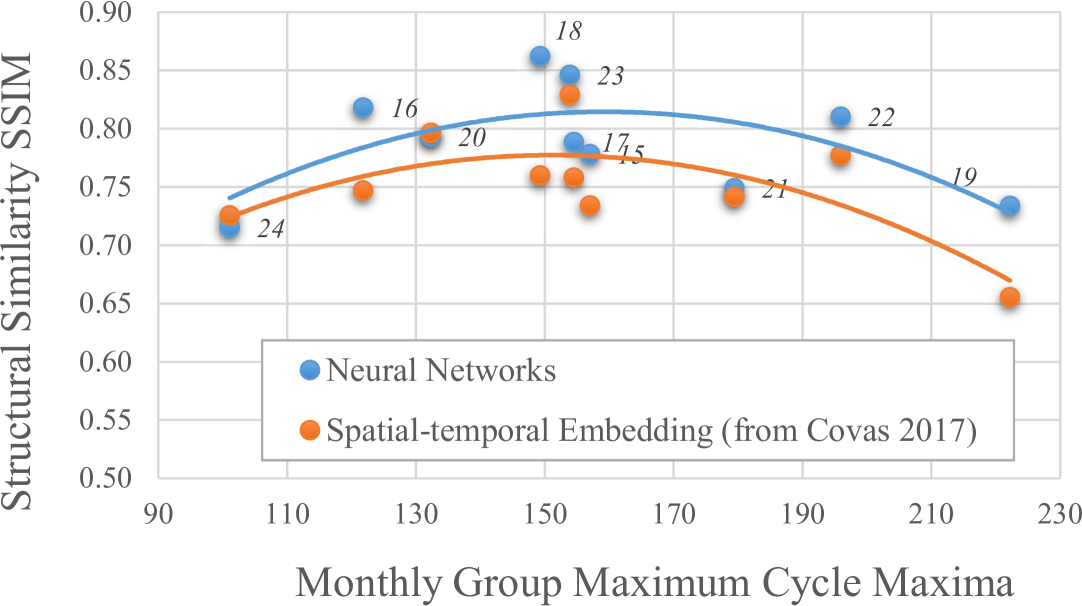
Figure 5.: The structural similarity, SSIM, of the prediction set versus the original test set against the cycle strength as given by the monthly group maximum sunspot number (Hathaway, 2015b). The plot labels represent the cycle number. The analysis shows that the approach is most accurate for medium amplitude cycles. Notice we have excluded attempts to predict Cycles 11 to 14 as for these cycles there is not enough past data (see Covas, 2017, for details). To increase the precision of the forecast, we took 20 million patterns per cycle, to compensate for the smaller average learning set lengths than in the previous figures. We compared our results against those in Covas (2017), who used a spatial-temporal non-linear embedding approach. There is a clear similarity in both methods, both being less effective for weak and strong cycles. Overall, we observe that the neural network approach has a small advantage over the spatial-temporal non-linear embedding approach.SSIM_versus_cycle_maxima

The results of our analysis are depicted in Figure SSIM_versus_cycle_maxima. There are three conclusions from analysing it.

First, the forecasting ability of the neural network increases as the number of temporal slices increases, and as a result SSIM metric improves a bit. This is a well known behaviour of neural networks, which are very data hungry, i.e. the larger the number of training patterns, the closer will the neural network internal parameters (i.e. the weights) be to the optimal theoretical values.

Second, and most importantly, the neural network approach achieves its higher performance for medium cycles, i.e. the most common cycles. We have, as in Covas (2017), fitted a parabola trend on it, that shows this clearly. We also compared and super-imposed the results in Covas (2017), who have used a non-linear embedding method. It seems to show that the neural network method is somehow slightly better at forecasting than the embedding method. However, neither of the methods is good enough as one could wish for weak or strong cycles. The neural network approach works on the basis of extracting knowledge from the training patterns. If there are not enough training examples tracing weak or strong cycles, then the weights will converge to values that tend to be biased towards medium cycles - the most common ones. There are two obvious ways, while using neural networks, to improve the accuracy of the forecasts. One is to gather more sunspot butterfly diagram data. This is not easy, as one either has to physically wait to grow the dataset, and given the average cycle has a rough periodicity of 11 years, one could be waiting a long time. Another way to collect more data is to use recently recovered sunspot butterfly diagram data going back to the early 18th century (see Figure 2 in Arlt, 2009 and Figure 1 in Usoskin et al., 2009). The other way to improve accuracy is to include extra data, or as commonly known in machine learning, extra features. There is a strong argument on using other datasets, such as geomagnetic data (Wang and Sheeley, 2009), solar magnetic fields datasets (Muñoz-Jaramillo, Balmaceda, and DeLuca, 2013), the so-called polar faculae (Muñoz-Jaramillo et al., 2012), and solar seismological data (Ilonidis, Zhao, and Hartlep, 2013). Nonetheless, it is outside the scope of this article to include further data. We note, however, that the neural network method allows the inclusion of other data easily as long as the temporal frequency of data points is the same as the sunspot data. We plan to pursue this research line in a forthcoming article. Here we have basically attempted to demonstrate the possibility of qualitatively forecasting using a pure mathematical method, that is, another approach to be added to the existing ones in the literature, such as the application of empirical relationships (Jiang et al., 2011; Santos et al., 2015; Cameron, Jiang, and Schüssler, 2016) or the ones using solar surface magnetic field datasets (McIntosh et al., 2014b, a; Jiang and Cao, 2018).

Third and finally, Figure SSIM_versus_cycle_maxima shows that the neural network method performs slightly better than the non-linear spatial-temporal embedding approach in Covas (2017). This is quite encouraging that this work is going in the right direction.

3.5 Further Forecasts

furtherforecasts

In this section, we examine further forecasts, outside our base training and testing set split we used above. In particular we wanted to understand the forecast of the most recent Cycle 24 and the future Cycle 25. We have seen from Figure SSIM_versus_cycle_maxima that the forecast of Cycle 24, a weak cycle, was not very good in terms of the SSIM index. In order to know if this is a general problem with this cycle, we plotted in Figure SolarForecastingNeuralNetworksSumOverLatitudeCycle24 two forecasts, one with the data up to Cycle 22 (inclusive) and used it to forecast Cycle 24 (by concatenation): the green line, i.e. exactly what we have done in Figure SolarForecastingNeuralNetworksSumOverLatitude, and one where we used the entire dataset up to Cycle 23 (inclusive) to forecast Cycle 24: the orange line. The results seem to show an improvement in terms of a more accurate cycle maximum amplitude (but not in terms of the actual cycle start). This improvement is due, presumably, because first, we used more data, and second, we do not attempt to forecast too ahead in time, a clear known problem with chaotic systems, even if this is thought to be a weakly chaotic system. The forecast with more data also compares well with other results in the literature (see Pesnell, 2016, and references therein). Our results are, of course, about sunspot areas. We can attempt to convert them into sunspot numbers by first, doing the same average or smoothing for the predicted sunspot areas (we shall call this $\bar{A}$) that is reported in the 13-month smoothed monthly sunspot number and, second, by noting the empirical relationship between sunspot areas (A) and the sunspot numbers (R) in Wilson and Hathaway (2006): $A/R\approx 13.6\times 0.6$, where the $0.6$ factor comes from the recalibration of international sunspot numbers introduced in July 2015 (Clette and Lefèvre, 2016). For the purpose of these calculations, we actually calculate an estimation of this empirical relationship ourselves, e.g. by calculating the average $\bar{A}/R$ for Cycles 22 and 23, where $A$ is the sunspot area per Carrington rotation number, $\bar{A}$ is the value of $A$ averaged or smoothed over 13 months, and $R$ is the 13-month smoothed monthly sunspot number. We obtain the value $\bar{A}/R\approx 9.40$ which compares well with the value from Wilson and Hathaway (2006), i.e. $A/R\approx 13.6\times 0.6\approx 8.16$.

This would imply, given our forecast of a Cycle 24 maximum 13-month smoothed sunspot area coverage of $\bar{A}_{24}=1521.66\pm 539.20$ (summed over latitudes), that Cycle 24 would have a maximum sunspot number of $R_{24}=161.86\pm 57.36$. The actual maximum according to the data in Sunspot Index and Long-Term Solar Observations (SILSO) World Data Center (1749-2018) occurred around April 2014 with the value $R_{24}=116.4$, based on 13-month smoothed monthly sunspot number data. Our value is within the error range, which is good, but our maximum shows up almost two years earlier than the real solar maximum. It is known that the Cycle 23 to 24 transition was an unusual low and long quiet period (Lockwood et al., 2012) and that without further data or external data it is probably not possible for the neural network method to forecast that unusual late start.

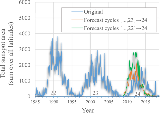
Figure 6.: Comparison of the latitudinal sum of the sunspot area $A(t)$ and the forecast for the current Cycle 24 using a training set that includes all the data up to Cycle 23 against the one as in Figure SolarForecastingNeuralNetworksSumOverLatitude. We have marked the cycle numbers near the horizontal axis. It seems to show that using more data improves the forecast, if not in terms of the onset of the cycle, at least in terms of the cycle maximum amplitude.SolarForecastingNeuralNetworksSumOverLatitudeCycle24

Finally, before we conclude, we attempted to forecast the forthcoming Cycle 25, using all the spatial-temporal data we have. The results can be seen in Figure SolarForecastingNeuralNetworksSumOverLatitude25. It seems to suggest that the next Cycle 25 will be around half of the intensity as the current one (Cycle 24), as measured by the sum of all sunspot areas (summed over the whole cycle and over all latitudes). This would imply, given our forecast of a Cycle 25 maximum 13-month smoothed sunspot area coverage of $\bar{A}_{25}=538.09\pm 157.51$ (summed over latitudes), that the next Cycle 25 will have a maximum sunspot number of $R_{25}=57.24\pm 16.76$. This suggests that this forthcoming Cycle 25 will be the weakest cycle in recorded history. As the saying goes, only time will tell. We also note that this value of $57.24$ is quite below the average of values seen in the Cycle 25 prediction literature (see Hathaway and Upton, 2016; Upton and Hathaway, 2018, and references therein).

Nonetheless, given our comments on the “piano plot” in the introduction, we do not want to put too much emphasis on this prediction, as we believe, based on that plot and on the fact that the cycle amplitude is a metric that sums over all the detailed information on the spatial-temporal diagram, that one should aim to compare the entire time and latitude forecast, and not just a numeric reduction of zero dimensionality such as the maximum sunspot number.

Figure 7.: Forecast of the latitudinal sum of the sunspot area $A(t)$ for the next Cycle 25 using a training set that includes all the data up to Cycle 24. We have marked the cycle numbers near the horizontal axis. It suggests the next cycle will be quite weak and peak around 2022–2023.SolarForecastingNeuralNetworksSumOverLatitude25

4 Conclusion

conclusion

We used the so-called feed-forward artificial neural network in an effort to forecast the solar sunspot butterfly diagram in space and time simultaneously. As far as we are aware, this is the first time this has been attempted using neural networks - all the work in the literature focus on using neural networks applied to pure sunspot temporal series, e.g. the average sunspot number or the sunspot area coverage. To contrast, here we attempt to use neural networks to predict sunspots both in time and space.

The results show that the method can reproduce qualitatively some of the main features of the sunspot diagram, such as the overall cycle amplitude modulation, and the cycle sunspot migration to the equator. However, there are limits to the forecast, namely the time horizon - the method does not seem to be able to forecast more than one cycle in advance, although this can be justified by the fact that the sunspot cycle is considered to be an example of a chaotic system, and therefore with a short predictability horizon. Also, the approach seems to be slightly biased towards medium cycles, the most common ones. This is clearly demonstrated in the analysis of the structure similarity index against the cycle strength. This is consistent on what was seen when using a non-linear embedding method in (Covas, 2017). In fact, there seems to be quite a parallel in the results of the two forecasting methods. Further to that, we also predict, based on our method, that the upcoming Cycle 25 maximum will be around $R_{25}=57\pm 17$. This implies that Cycle 25 will be the weakest cycle on record.

We also found that the spatial-temporal non-linear embedding method in (Parlitz and Merkwirth, 2000) points the way for the optimal input layer representation for neural network forecasting, an empirical result that may show there is some general-purpose theorem waiting to be demonstrated. We plan to demonstrate this potential universality using other datasets in a forthcoming article.

We believe that the work points in the right direction, first that we ought to attempt to forecast in space as well as in time, and second that further improvements ought to be tried. The first improvement must surely be to use recurrent networks, such as Elman networks (Elman, 1990) which are known to be more appropriate to model time series (although more complex to design and construct, hence why we started with simple and understandable feed-forward neural networks). The second improvement that we suggest is to incorporate related information as additional input(s), e.g.  to use solar magnetic field proxies such as the 10.7 cm radio flux and the 530.3 nm green coronal index (Broomhall and Nakariakov, 2015), and even geomagnetic proxies such as the aa indices (Mayaud, 1972; Nevanlinna and Kataja, 1993), as these are also long time series with similar or higher temporal frequency than the dataset we have used. In this article we wanted to focus on showing that neural networks can qualitatively model both the spatial and the temporal dynamics of the sunspot diagram and we plan to revisit the improvements mentioned above in future work.

Overall we think forecasting in higher dimensions, particularly using neural networks and deep learning, even if it is harder computationally and more demanding in terms of the size of the data used, should point to other research possibilities within solar physics and within the emerging field of space weather.

Acknowledgments

We would like to thank Reza Tavakol for very useful conversations regarding forecasting sunspots. We also would like to thank Dr. David Hathaway for publishing the data that we used in this article. Finally, we would also like to thank the anonymous reviewer, whose comments have helped to improve this article. N. Peixinho acknowledges funding from the Portuguese FCT – Foundation for Science and Technology (ref: SFRH/ BGCT/ 113686/ 2015). CITEUC is funded by National Funds through FCT – Foundation for Science and Technology (project: UID/ Multi/ 00611/ 2013) and FEDER – European Regional Development Fund through COMPETE 2020 – Operational Programme Competitiveness and Internationalisation (project: POCI-01-0145-FEDER-006922). J. Fernandes acknowledges funding from the POCH and Portuguese FCT – Foundation for Science and Technology (ref: SFRH/BSAB/143060/2018) and visiting facilities at Niels Bohr Institute (University of Copenhagen).

Disclosure of Potential Conflicts of Interest

The authors declare to have no conflicts of interest.

References

- Abarbanel and Gollub (1996) Abarbanel, H.D.I., Gollub, J.P.: 1996, Analysis of Observed Chaotic Data. Phys. Today 49, 86. DOI. ADS.
- Acero et al. (2017) Acero, F.J., Carrasco, V.M.S., Gallego, M.C., García, J.A., Vaquero, J.M.: 2017, Extreme Value Theory and the New Sunspot Number Series. ApJ 839, 98. DOI. ADS.
- Arlt (2009) Arlt, R.: 2009, The Butterfly Diagram in the Eighteenth Century. Sol. Phys. 255, 143. DOI. ADS.
- Arlt and Weiss (2014) Arlt, R., Weiss, N.: 2014, Solar Activity in the Past and the Chaotic Behaviour of the Dynamo. Space Sci. Rev. 186, 525. DOI. ADS.
- Ashwin, Covas, and Tavakol (1999) Ashwin, P., Covas, E., Tavakol, R.: 1999, Transverse instability for non-normal parameters. Nonlinearity 12, 563. DOI. ADS.
- Beer, Tobias, and Weiss (1998) Beer, J., Tobias, S., Weiss, N.: 1998, An Active Sun Throughout the Maunder Minimum. Sol. Phys. 181, 237. DOI. ADS.
- Broomhall and Nakariakov (2015) Broomhall, A.-M., Nakariakov, V.M.: 2015, A Comparison Between Global Proxies of the Sun’s Magnetic Activity Cycle: Inferences from Helioseismology. Sol. Phys. 290, 3095. DOI. ADS.
- Cameron, Jiang, and Schüssler (2016) Cameron, R.H., Jiang, J., Schüssler, M.: 2016, Solar Cycle 25: Another Moderate Cycle? ApJ 823, L22. DOI. ADS.
- Chandra and Zhang (2012) Chandra, R., Zhang, M.: 2012, Cooperative coevolution of elman recurrent neural networks for chaotic time series prediction. Neurocomputing 86, 116. DOI.
- Cheng et al. (2014) Cheng, T., Wang, J., Haworth, J., Heydecker, B., Chow, A.: 2014, A dynamic spatial weight matrix and localized space-time autoregressive integrated moving average for network modeling. Geogr. Anal. 46(1), 75. DOI.
- Clette and Lefèvre (2016) Clette, F., Lefèvre, L.: 2016, The New Sunspot Number: Assembling All Corrections. Sol. Phys. 291(9-10), 2629. DOI.
- Covas (2017) Covas, E.: 2017, Spatial-temporal forecasting the sunspot diagram. A&A 605, A44. DOI. ADS.
- Covas and Mena (2011) Covas, E.O., Mena, F.C.: 2011, Forecasting of yield curves using local state space reconstruction. In: Dynamics, Games and Science I, Springer Berlin Heidelberg, 243. DOI.
- Cun, Denker, and Solla (1990) Cun, Y.L., Denker, J.S., Solla, S.a.: 1990, Optimal Brain Damage. Advances in Neural Information Processing Systems. 1558601007. DOI.
- David E.; McClelland (1989) David E.; McClelland, J.L.R.: 1989, Parallel distributed processing: Explorations in the microstructure of cognition; vol. 1: Foundations, The MIT Press. ISBN 0262181207.
- Elman (1990) Elman, J.L.: 1990, Finding structure in time. Cognitive Science 14(2), 179. DOI.
- Frank, Davey, and Hunt (2001) Frank, R.J., Davey, N., Hunt, S.P.: 2001, Time series prediction and neural networks. J. Intell. Rob. Syst. 31(1), 91. DOI.
- Fraser and Swinney (1986) Fraser, A.M., Swinney, H.L.: 1986, Independent coordinates for strange attractors from mutual information. Phys. Rev. A 33(2), 1134. DOI.
- Hale (1908) Hale, G.E.: 1908, On the Probable Existence of a Magnetic Field in Sun-Spots. ApJ 28, 315. DOI. ADS.
- Han et al. (2004) Han, M., Xi, J., Xu, S., Yin, F.-L.: 2004, Prediction of chaotic time series based on the recurrent predictor neural network. IEEE Transactions on Signal Processing 52(12), 3409. DOI.
- (21) Hassibi, B., Stork, D.G., Wolff, G.J.: Optimal brain surgeon and general network pruning. In: IEEE International Conference on Neural Networks, IEEE. DOI.
- Hathaway (2015a) Hathaway, D.H.: 2015a, Sunspot area butterfly diagram data. Original data in http://solarscience.msfc.nasa.gov/greenwch.shtml and more up-to-date data in http://solarcyclescience.com/activeregions.html.
- Hathaway (2015b) Hathaway, D.H.: 2015b, The Solar Cycle. Living Rev. Sol. Phys. 12, 4. DOI. ADS.
- Hathaway and Upton (2016) Hathaway, D.H., Upton, L.A.: 2016, Predicting the amplitude and hemispheric asymmetry of solar cycle 25 with surface flux transport. Journal of Geophysical Research: Space Physics 121(11), 10,744. DOI.
- Hathaway et al. (2003) Hathaway, D.H., Nandy, D., Wilson, R.M., Reichmann, E.J.: 2003, Evidence That a Deep Meridional Flow Sets the Sunspot Cycle Period. ApJ 589, 665. DOI. ADS.
- Ilonidis, Zhao, and Hartlep (2013) Ilonidis, S., Zhao, J., Hartlep, T.: 2013, Helioseismic Investigation of Emerging Magnetic Flux in the Solar Convection Zone. ApJ 777, 138. DOI. ADS.
- Ivanov and Miletsky (2011) Ivanov, V.G., Miletsky, E.V.: 2011, Width of Sunspot Generating Zone and Reconstruction of Butterfly. Sol. Phys. 268, 231. DOI. ADS.
- Jiang and Cao (2018) Jiang, J., Cao, J.: 2018, Predicting solar surface large-scale magnetic field of Cycle 24. J. Atmos. Sol. Terr. Phys. 176, 34. DOI. ADS.
- Jiang et al. (2011) Jiang, J., Cameron, R.H., Schmitt, D., Schüssler, M.: 2011, The solar magnetic field since 1700. I. Characteristics of sunspot group emergence and reconstruction of the butterfly diagram. A&A 528, A82. DOI. ADS.
- Kennel, Brown, and Abarbanel (1992) Kennel, M.B., Brown, R., Abarbanel, H.D.I.: 1992, Determining embedding dimension for phase-space reconstruction using a geometrical construction. Phys. Rev. A 45, 3403. DOI. ADS.
- Kim, Eykholt, and Salas (1999) Kim, H.S., Eykholt, R., Salas, J.D.: 1999, Nonlinear dynamics, delay times, and embedding windows. Physica D Nonlinear Phenomena 127, 48. DOI. ADS.
- Krizhevsky, Sutskever, and Hinton (2017) Krizhevsky, A., Sutskever, I., Hinton, G.E.: 2017, ImageNet classification with deep convolutional neural networks. Communications of the ACM 60(6), 84. DOI.
- Lecun et al. (1998) Lecun, Y., Bottou, L., Bengio, Y., Haffner, P.: 1998, Gradient-based learning applied to document recognition. Proceedings of the IEEE 86(11), 2278. DOI.
- Letellier et al. (2006) Letellier, C., Aguirre, L.A., Maquet, J., Gilmore, R.: 2006, Evidence for low dimensional chaos in sunspot cycles. A&A 449, 379. DOI. ADS.
- Lockwood et al. (2012) Lockwood, M., Owens, M., Barnard, L., Davis, C., Thomas, S.: 2012, Solar cycle 24: what is the sun up to? Astronomy & Geophysics 53(3), 3.09. DOI.
- Lu et al. (2017) Lu, Z., Pathak, J., Hunt, B., Girvan, M., Brockett, R., Ott, E.: 2017, Reservoir observers: Model-free inference of unmeasured variables in chaotic systems. Chaos 27(4), 041102. DOI. ADS.
- Luk, Ball, and Sharma (2000) Luk, K.C., Ball, J.E., Sharma, A.: 2000, A study of optimal model lag and spatial inputs to artificial neural network for rainfall forecasting. J. Hydrol. 227(1-4), 56. DOI.
- Luthardt and Rößler (2017) Luthardt, L., Rößler, R.: 2017, Fossil forest reveals sunspot activity in the early Permian. Geology 45, 279. DOI. ADS.
- Mayaud (1972) Mayaud, P.-N.: 1972, The aa indices: A 100-year series characterizing the magnetic activity. J. Geophys. Res. 77, 6870. DOI. ADS.
- McDermott and Wikle (2017) McDermott, P.L., Wikle, C.K.: 2017, An ensemble quadratic echo state network for non-linear spatio-temporal forecasting. Stat. 6(1), 315. DOI.
- McIntosh et al. (2014a) McIntosh, S.W., Wang, X., Leamon, R.J., Davey, A.R., Howe, R., Krista, L.D., Malanushenko, A.V., Markel, R.S., Cirtain, J.W., Gurman, J.B., Pesnell, W.D., Thompson, M.J.: 2014a, Deciphering Solar Magnetic Activity. I. On the Relationship between the Sunspot Cycle and the Evolution of Small Magnetic Features. ApJ 792, 12. DOI. ADS.
- McIntosh et al. (2014b) McIntosh, S.W., Wang, X., Leamon, R.J., Scherrer, P.H.: 2014b, Identifying Potential Markers of the Sun’s Giant Convective Scale. ApJ 784, L32. DOI. ADS.
- Muñoz-Jaramillo, Balmaceda, and DeLuca (2013) Muñoz-Jaramillo, A., Balmaceda, L.A., DeLuca, E.E.: 2013, Using the Dipolar and Quadrupolar Moments to Improve Solar-Cycle Predictions Based on the Polar Magnetic Fields. Phys. Rev. Lett. 111(4), 041106. DOI. ADS.
- Muñoz-Jaramillo et al. (2012) Muñoz-Jaramillo, A., Sheeley, N.R., Zhang, J., DeLuca, E.E.: 2012, Calibrating 100 Years of Polar Faculae Measurements: Implications for the Evolution of the Heliospheric Magnetic Field. ApJ 753, 146. DOI. ADS.
- Mundt, Maguire, and Chase (1991) Mundt, M.D., Maguire, W.B. II, Chase, R.R.P.: 1991, Chaos in the sunspot cycle - Analysis and prediction. J. Geophys. Res. 96, 1705. DOI. ADS.
- Nevanlinna and Kataja (1993) Nevanlinna, H., Kataja, E.: 1993, An extension of the geomagnetic activity index series aa for two solar cycles (1844-1868). Geophys. Res. Lett. 20, 2703. DOI. ADS.
- Oh (2002) Oh, K.: 2002, Analyzing stock market tick data using piecewise nonlinear model. Expert Syst. Appl. 22(3), 249. DOI.
- Owens (2013) Owens, B.: 2013, Long-term research: Slow science. Nature 495, 300. DOI. ADS.
- Parlitz and Merkwirth (2000) Parlitz, U., Merkwirth, C.: 2000, Prediction of Spatiotemporal Time Series Based on Reconstructed Local States. Phys. Rev. Lett. 84, 1890. DOI. ADS.
- Pathak et al. (2017) Pathak, J., Lu, Z., Hunt, B.R., Girvan, M., Ott, E.: 2017, Using machine learning to replicate chaotic attractors and calculate Lyapunov exponents from data. Chaos 27(12), 121102. DOI. ADS.
- Pathak et al. (2018) Pathak, J., Wikner, A., Fussell, R., Chandra, S., Hunt, B.R., Girvan, M., Ott, E.: 2018, Hybrid forecasting of chaotic processes: Using machine learning in conjunction with a knowledge-based model. Chaos 28(4), 041101. DOI. ADS.
- Pathak et al. (2018) Pathak, J., Hunt, B., Girvan, M., Lu, Z., Ott, E.: 2018, Model-free prediction of large spatiotemporally chaotic systems from data: A reservoir computing approach. Phys. Rev. Lett. 120, 024102. DOI.
- Pesnell (2008) Pesnell, W.D.: 2008, Predictions of solar cycle 24. Sol. Phys. 252(1), 209. DOI.
- Pesnell (2012) Pesnell, W.D.: 2012, Solar Cycle Predictions (Invited Review). Sol. Phys. 281, 507. DOI. ADS.
- Pesnell (2016) Pesnell, W.D.: 2016, Predictions of solar cycle 24: How are we doing? Space Weather 14(1), 10. DOI.
- Petrosian et al. (2000) Petrosian, A., Prokhorov, D., Homan, R., Dasheiff, R., Wunsch, D.: 2000, Recurrent neural network based prediction of epileptic seizures in intra- and extracranial EEG. Neurocomputing 30(1-4), 201. DOI.
- Raissi (2018) Raissi, M.: 2018, Deep Hidden Physics Models: Deep Learning of Nonlinear Partial Differential Equations. ArXiv e-prints. ADS.
- Raissi and Karniadakis (2018) Raissi, M., Karniadakis, G.E.: 2018, Hidden physics models: Machine learning of nonlinear partial differential equations. J. Comput. Phys. 357, 125. DOI. ADS.
- Raissi, Perdikaris, and Karniadakis (2017a) Raissi, M., Perdikaris, P., Karniadakis, G.E.: 2017a, Physics Informed Deep Learning (Part I): Data-driven Solutions of Nonlinear Partial Differential Equations. ArXiv e-prints. ADS.
- Raissi, Perdikaris, and Karniadakis (2017b) Raissi, M., Perdikaris, P., Karniadakis, G.E.: 2017b, Physics Informed Deep Learning (Part II): Data-driven Discovery of Nonlinear Partial Differential Equations. ArXiv e-prints. ADS.
- Reed (1999) Reed, R.: 1999, Neural smithing: Supervised learning in feedforward artificial neural networks (a bradford book), A Bradford Book. ISBN 0262527014.
- Rumelhart, Hinton, and Williams (1986) Rumelhart, D.E., Hinton, G.E., Williams, R.J.: 1986, Learning representations by back-propagating errors. Nature 323, 533. DOI. ADS.
- Santos et al. (2015) Santos, A.R.G., Cunha, M.S., Avelino, P.P., Campante, T.L.: 2015, Spot cycle reconstruction: an empirical tool. Application to the sunspot cycle. A&A 580, A62. DOI. ADS.
- Schwabe (1844) Schwabe, H.: 1844, Sonnenbeobachtungen im Jahre 1843. Von Herrn Hofrath Schwabe in Dessau. Astron. Nachr. 21, 233. DOI. ADS.
- Sheng et al. (2003) Sheng, Z., Hong-Xing, L., Dun-Tang, G., Si-Dan, D.: 2003, Determining the input dimension of a neural network for nonlinear time series prediction. Chin. Phys. 12(6), 594. DOI.
- Solanki et al. (2004) Solanki, S.K., Usoskin, I.G., Kromer, B., Schüssler, M., Beer, J.: 2004, Unusual activity of the Sun during recent decades compared to the previous 11,000 years. Nature 431, 1084. DOI. ADS.
- Spiegel (2009) Spiegel, E.A.: 2009, Chaos and Intermittency in the Solar Cycle. Space Sci. Rev. 144, 25. DOI. ADS.
- Stathakis (2009) Stathakis, D.: 2009, How many hidden layers and nodes? Int. J. Remote Sens. 30(8), 2133. DOI.
- Sunspot Index and Long-Term Solar Observations (SILSO) World Data Center (1749-2018) Sunspot Index and Long-Term Solar Observations (SILSO) World Data Center: 1749-2018, The international sunspot number, 13-month smoothed monthly sunspot number in http://sidc.be/silso/DATA/SN_ms_tot_V2.0.txt. International Sunspot Number Monthly Bulletin and online catalogue. ADS.
- Upton and Hathaway (2018) Upton, L.A., Hathaway, D.H.: 2018, An Updated Solar Cycle 25 Prediction With AFT: The Modern Minimum. Geophys. Res. Lett. 45(16), 8091. DOI.
- Usoskin et al. (2009) Usoskin, I.G., Mursula, K., Arlt, R., Kovaltsov, G.A.: 2009, A Solar Cycle Lost in 1793-1800: Early Sunspot Observations Resolve the Old Mystery. ApJ 700, L154. DOI. ADS.
- Waibel et al. (1990) Waibel, A., Hanazawa, T., Hinton, G., Shikano, K., Lang, K.J.: 1990, Phoneme recognition using time-delay neural networks. In: Readings in Speech Recognition, Elsevier, 393. DOI.
- Wang and Sheeley (2009) Wang, Y.-M., Sheeley, N.R.: 2009, Understanding the Geomagnetic Precursor of the Solar Cycle. ApJ 694, L11. DOI. ADS.
- Wang et al. (2004) Wang, Z., Bovik, A.C., Sheikh, H.R., Simoncelli, E.P.: 2004, Image quality assessment: From error visibility to structural similarity. IEEE Transactions on Image Processing 13(4), 600. DOI.
- Weiss (1988) Weiss, N.O.: 1988, Is the solar cycle an example of deterministic chaos? In: Stephenson, F.R., Wolfendale, A.W. (eds.) Secular Solar and Geomagnetic Variations in the Last 10,000 Years,, 69. ADS.
- Weiss (1990) Weiss, N.O.: 1990, Periodicity and Aperiodicity in Solar Magnetic Activity. Philosophical Transactions of the Royal Society of London Series A 330, 617. DOI. ADS.
- Wilson and Martinez (2003) Wilson, D.R., Martinez, T.R.: 2003, The general inefficiency of batch training for gradient descent learning. Neural Networks 16(10), 1429. DOI.
- Wilson and Hathaway (2006) Wilson, R.M., Hathaway, D.H.: 2006, On the Relation Between Sunspot Area and Sunspot Number. NASA STI/Recon Technical Report N 6. ADS.
- Zhang and Xiao (2000) Zhang, J.-S., Xiao, X.-C.: 2000, Predicting chaotic time series using recurrent neural network. Chin. Phys. Lett. 17(2), 88. DOI.
- Zhang (2009) Zhang, Y.: 2009, Recurrent neural networks: Design, analysis, applications to control and robotic systems, LAP Lambert Academic Publishing. ISBN 3838303822.