Convexification of a 3-D coefficient inverse scattering problem

Abstract

A version of the so-called “convexification” numerical method for a coefficient inverse scattering problem for the 3D Hemholtz equation is developed analytically and tested numerically. Backscattering data are used, which result from a single direction of the propagation of the incident plane wave on an interval of frequencies. The method converges globally. The idea is to construct a weighted Tikhonov-like functional. The key element of this functional is the presence of the so-called Carleman Weight Function (CWF). This is the function which is involved in the Carleman estimate for the Laplace operator. This functional is strictly convex on any appropriate ball in a Hilbert space for an appropriate choice of the parameters of the CWF. Thus, both the absence of local minima and convergence of minimizers to the exact solution are guaranteed. Numerical tests demonstrate a good performance of the resulting algorithm. Unlikeprevious the so-called tail functions globally convergent method, we neither do not impose the smallness assumption of the interval of wavenumbers, nor we do not iterate with respect to the so-called tail functions.

Keywords: coefficient inverse scattering problem, Carleman weight function, globally convergent numerical method

2010 Mathematics Subject Classification: 35R30.

1 Introduction

In this work, we develop a version of the so-called “convexification” numerical method for a coefficient inverse scattering problem (CISP) for the 3D Helmholtz equation with backscattering data resulting from a single measurement event which is generated by a single direction of the propagation of the incident plane wave on an interval of frequencies. We present both the theory and numerical results. Our method converges globally. This is a generalization to the 3D case of our (with coauthors) previous 1D version of the convexification [1]. Three main advantages of the convexification method over the previously developed the so-called “tail functions” globally convergent method for a similar CISP [2, 3, 4, 5, 6, 7] are: (1) To solve our problem, we construct a globally strictly convex cost functional with the Carleman Weight Function (CWF) in it, (2) we do not impose in our convergence analysis the smallness assumption on the interval of wavenumbers, and (3) we do not iterate with respect to the so-called “tail functions”.

It is well known that any CISP is both highly nonlinear and ill-posed. These two factors cause substantial difficulties in numerical solutions of these problems. A globally convergent method (GCM) for a CISP is such a numerical method, which has a rigorous guarantee of reaching a sufficiently small neighborhood of the exact solution of that CISP without any advanced knowledge of this neighborhood. In addition, the size of this neighborhood should depend only on approximation errors and the level of noise in the data.

Over the years the first author with coauthors has proposed a variety of globally convergent methods for CISPs with single measurement data, see, e.g. [2, 3, 4, 5, 7, 8, 9, 10, 11, 12, 13, 14, 15], and references cited therein. These methods can be classified into two types. Methods of the first type, which we call the tail functions methods, are certain iterative processes. On each iterative step one solves the Dirichlet boundary value problem for a linear elliptic Partial Differential Equation (PDE). This PDE depends on the iteration number. The solution of that problem enables one to update the unknown coefficient. Using this update, one updates the so-called tail function, which is a complement of a certain truncated integral, where the integration is carried out with respect to the wavenumber. The stopping criterion for the iterative process is developed computationally. The tail function method was successfully tested on experimental backscattering data The tail function method was successfully tested on experimental backscattering data [4, 5, 6, 7, 14].

Globally convergent numerical methods of the second type are called the convexification methods. They are based on the minimization of the weighted Tikhonov-like functional with the CWF in it. The CWF is the function which is involved in the Carleman estimate for the corresponding PDE operator. The CWF can be chosen in such a way that the above functional becomes strictly convex on a ball of an arbitrary radius in a certain Hilbert space (see some details in this section below). Note that the majority of known numerical methods of solutions of nonlinear ill-posed problems minimize conventional least squares cost functionals [16, 17, 18], which are usually non convex and have multiple local minima and ravines, see, e.g. [19] for a good numerical example of multiple local minima. Hence, a gradient-like method for such a functional converges to the exact solution only if the starting point of iterations is located in a sufficiently small neighborhood of this solution. Some other effective approache to numerical methods for nonlinear ill-posed problems can be found in [20, 21].

Various versions of the convexification methods have been proposed since the first work [9], see [10, 11, 12]. However, these versions have some theoretical gaps, which have limited their numerical studies so far. In the recent works [8, 13, 22] the attention to the convexification method was revived. Theoretical gaps were eliminated in [23] and thorough numerical studies for one dimensional problems were performed [1, 15]. Besides, in [24] the convexification method was developed for ill-posed problems for quasilinear PDEs and corresponding numerical studies for the 1D case were conducted in [22, 23]. The idea of any version of the convexification has direct roots in the method of [25], which is based on Carleman estimates. The method of [25] was originally designed only for proofs of uniqueness theorems for CIPs, also see, e.g. the book [12] and the recent survey [26]. Recently an interesting version of the convexification was published in [27] for a CISP for the hyperbolic equation $u_{tt}=\Delta u+a\left(x\right)u$ with the unknown coefficient $a\left(x\right)$ in the case when one of initial conditions does not non-vanish. The method of [27] is also based on the idea of [25] and has some roots in [8, 13].

By the convexification, one constructs a weighted Tikhonov-like functional $J_{\lambda}$ on a closed ball $\overline{B\left(R\right)}$ of an arbitrary radius $R>0$ and with the center at $\left\{0\right\}$ in an appropriate Hilbert space. Here $\lambda>0$ is a parameter. The key theorem claims that one can choose a number $\lambda\left(R\right)>0$ such that for all $\lambda\geq\lambda\left(R\right)$ the functional $J_{\lambda}$ is strictly convex on $\overline{B\left(R\right)}.$ Furthermore, the existence of the unique minimizer of $J_{\lambda}$ on $\overline{B\left(R\right)}$ as well as convergence of minimizers to the exact solution when the level of noise in the data tends to zero are proven. In addition, it is proven that the gradient projection method reaches a sufficiently small neighborhood of the exact coefficient when starting from an arbitrary point of $B\left(R\right)$. Since $R>0$ is an arbitrary number, then this is a globally convergent numerical method.

Due to a broad variety of applications, Inverse Scattering Problems (ISPs) are quite popular in the community of experts in inverse problems. There are plenty of works dedicated to this topic. Since this paper is not a survey, we refer to only few of them, e.g. [17, 18, 20, 21, 28, 29, 30, 31, 32, 33, 34, 35, 36, 37, 38, 39, 40, 41, 42, 43] and references cited thereein. We note that the authors of [33] have considered a modified tail functions method. As stated above, we are interested in a CISP for the Helmholtz equation with the data generated by a single measurement event. As to the CISPs with multiple measurements, we refer to a global reconstruction procedure, which was developed and numerically implemented in [37], also see [38, 39] for further developments and numerical studies. Actually, this is an effective extension of the classical 1D Gelfand-Krein-Levitan method on the 2D case.

In section 2 we formulate our forward and inverse problems. In section 3 we construct the weighted Tikhonov-like functional with the CWF in it. In section 4 we formulate our theorems.  We prove them in section 5. In section 6 we present numerical results.

2 Problem Statement

2.1 The Helmholtz equation

Just as in the majority of the above cited previous works of the first author with coauthors about GCM, we focus in this paper applications to the detection and identification of targets, which mimic antipersonnel land mines (especially plastic mines, i.e. dielectrics) and improvised explosive devices (IEDs) using measurements of a single component of the electric wave field. In this case the medium is assumed to be non magnetic, non absorbing, and the dielectric constant in it should be represented by a function, which is mostly a constant with some small sharp inclusions inside (however, we do not assume in our theory such a structure of the dielectric constant). These inclusions model antipersonnel land mines and IEDs. Suppose that the incident electric field has only one non zero component. It was established numerically in [44] that the propagation of that component through such a medium is well governed by the Helmholtz equation rather than by the full Maxwell’s system. Besides, in all above cited works of the first author with coauthors about experimental data those targets were accurately imaged by the above mentioned tail functions GCM using experimentally measured single component of the electric field and modeling the propagation of that component by the Helmholtz equation. In addition, we are unaware about a GCM for a CISP with single measurement data for the Maxwell’s system. Thus, we use the Helmholtz equation below.

The need of the detection and identification of, e.g. land mines, might, in particular, occur on a battlefield. Due to the security considerations, the amount of collected data should be small in this case, and these should be the backcattering data. Thus, we use only a single direction of the propagation of the incident plane wave of the electric field and assume measurements of only the backscattering part of the corresponding component of that field.

2.2 Forward and inverse problems

Let $\mathbf{x}=(x,y,z)\in\mathbb{R}^{3}$. Let $b,d,\xi>0$ be three numbers. It is convenient for our numerical studies (section 6) to define from the beginning the domain of interest $\Omega$ and the backscattering part $\Gamma$ of its boundary as

$$\Omega=\left\{\left(x,y,z\right):\left|x\right|,\left|y\right|<b,z\in\left(-\xi,d\right)\right\},\text{ }\Gamma=\left\{\left(x,y,z\right):\left|x\right|,\left|y\right|<b,z=-\xi\right\}.$$ (2.1)

Let the function $c(\mathbf{x})$ be the spatially distributed dielectric constant and $k$ be the wavenumber. We consider the following forward problem for the Helmholtz equation:

$$\Delta u+k^{2}\,c(\mathbf{x})\,u=0,\quad\mathbf{x}\in\mathbb{R}^{3},$$ (2.2)

$$u\left(\mathbf{x},k\right)=u_{s}\left(\mathbf{x},k\right)+u_{i}\left(\mathbb{x},k\right),$$ (2.3)

where $u(\mathbf{x},k)$ is the total wave, $u_{s}(\mathbf{x},k)$ is the scattered wave, and $u_{i}(\mathbf{x},k)$ is the incident plane wave propagating along the positive direction of the $z-$axis,

$$u_{i}(\mathbf{x},k)=e^{ikz}.$$ (2.4)

The scattered wave $u_{s}(\mathbf{x},k)$ satisfies the Sommerfeld radiation condition:

$$\lim_{r\rightarrow\infty}r\left(\frac{\partial u_{s}}{\partial r}-iku_{s}\right)=0,\quad r=\left|\mathbf{x}\right|.$$ (2.5)

Also, the function $c(\mathbf{x})$ satisfies the following conditions:

$$c(\mathbf{x})=1+\beta\left(\mathbf{x}\right),\text{ }\beta\left(\mathbf{x}\right)\geq 0,\,\mathbf{x}\in\mathbb{R}^{3},\quad\mbox{and}c(\mathbf{x})=1,\,\mathbf{x}\notin\overline{\Omega}.$$ (2.6)

The assumption of (2.6) $c(\mathbf{x})=1$ in $\mathbb{R}^{3}\setminus\Omega$ means that we have vacuum outside of the domain $\Omega.$ Finally, we assume that $c(\mathbf{x})\in C^{15}(\mathbb{R}^{3})$. This smoothness condition was imposed to derive the asymptotic behavior of the solution of the Helmholtz equation (2.2) at $k\rightarrow\infty$ [45]. We also note that extra smoothness conditions are usually not of a significant concern when a CIP is considered, see, e.g. theorem 4.1 in [46]. In particular, this smoothness condition implies that the function $u\left(\mathbf{x},k\right)\in C^{16+\gamma}\left(\overline{G}\right),\forall\gamma\in\left(0,1\right),\forall k>0,$ where $C^{16+\gamma}\left(\overline{G}\right)$ is the Hölder space and $G\subset\mathbb{R}^{3}$ is an arbitrary bounded domain [47]. Also, it follows from lemma 3.3 of [4] that the derivative $\partial_{k}u\left(\mathbf{x},k\right)$ exists for all $\mathbf{x}\in\mathbb{R}^{3},k>0$ and satisfies the same smoothness condition as the function $u\left(\mathbf{x},k\right).$

Coefficient Inverse Scattering Problem (CISP). Let the domain $\Omega$ and the backscattering part $\Gamma\subset\partial\Omega$ of its boundary be as in (2.1). Let the wavenumber $k\in[\underline{k},\overline{k}],$ where $[\underline{k},\overline{k}]$$\subset\left(0,\infty\right)$ is an interval of wavenumbers. Determine the function $c(\mathbf{x}),\,\mathbf{x}\in\Omega$, assuming that the following function $g(\mathbf{x},k)$ is given:

$$u(\mathbf{x},k)=g_{0}(\mathbf{x},k),\quad\mathbf{x}\in\Gamma,\,k\in[\underline{k},\overline{k}].$$ (2.7)

In addition to the data (2.7) we can obtain the boundary conditions for the derivative of the function $u(\mathbf{x},k)$ in the $z-$direction using the data propagation procedure (section 6.2),

$$u_{z}(\mathbf{x},k)=g_{1}(\mathbf{x},k),\quad\mathbf{x}\in\Gamma,\,k\in[\underline{k},\overline{k}].$$ (2.8)

In addition, we complement Dirichlet (2.7) and Neumann (2.8) boundary conditions on $\Gamma$ with the heuristic Dirichlet boundary condition at the rest of the boundary $\partial\Omega$ as:

$$u(\mathbf{x},k)=e^{ikz},\mathbf{x}\in\partial\Omega\diagdown\Gamma,\,k\in[\underline{k},\overline{k}].$$ (2.9)

This boundary condition coincides with the one for the uniform medium with $c\left(\mathbf{x}\right)\equiv 1.$ To justify (2.9), we recall that, using the tail functions method, it was demonstrated in sections 7.6 and 7.7 of [4] that (2.9) does not affect much the reconstruction accuracy as compared with the correct Dirichlet boundary condition. Besides, (2.9) has always been used in works [4, 5, 6, 7] with experimental data, where accurate results were obtained by the tail functions GCM.

The uniqueness of the solution of this CISP is an open and long standing problem. In fact, uniqueness of a similar coefficient inverse problem can be currently proven only in the case if the right hand side of equation (2.2) is a function which is not vanishing in $\overline{\Omega}.$ This can be done by the method of [25, 12, 26]. Hence, we assume below the uniqueness of our CISP.

2.3 Travel time

The Riemannian metric generated by the function $c(\mathbf{x})$ is:

$$d\tau(\mathbf{x})=\sqrt{c(\mathbf{x})}|d\mathbf{x}|,\quad|d\mathbf{x}|=\sqrt{(dx)^{2}+(dy)^{2}+(dz)^{2}}.$$

Fix the number $a>0.$ Consider the plane $P_{a}=\{(x,y,-a):x,y\in\mathbb{R}\}.$ We assume that $\Omega\subset\left\{z>-a\right\}$ and impose everywhere below the following condition on the function $c(\mathbf{x})$:

Regularity Assumption. For any point $x\in\mathbb{R}^{3}$ there exists a unique geodesic line $\Gamma(x,a)$, with respect to the metric $d\tau$, connecting $x$ with the plane $P_{a}$ and perpendicular to $P_{a}$.

A sufficient condition of the regularity of geodesic lines is [48]:

$$\sum_{i,j=1}^{3}\frac{\partial^{2}c\left(\mathbf{x}\right)}{\partial x_{i}\partial x_{j}}\xi_{i}\xi_{j}\geq 0,\forall\mathbf{x}\in\overline{\Omega},\forall\mathbf{\xi}\in\mathbb{R}^{3}.$$

We introduce the travel time $\tau(\mathbf{x})$ from the plane $P_{a}$ to the point $\mathbf{x}$ as [45]

$$\tau(\mathbf{x})=\int_{\Gamma(\mathbf{x},a)}\sqrt{c\left(\mathbf{\xi}\right)}d\sigma.$$

3 The Weighted Tikhonov Functionals

3.1 The asymptotic behavior

It was proven in [45] that the following asymptotic behavior of the function $u(\mathbf{x},k)$ is valid:

$$u(\mathbf{x},k)=A(\mathbf{x})e^{ik\tau(\mathbf{x})}\left[1+s\left(\mathbf{x},k\right)\right],\text{ }\mathbf{x}\in\overline{\Omega},k\rightarrow\infty,$$ (3.1)

where the function $s\left(\mathbf{x},k\right)$ is such that

$$s\left(\mathbf{x,}k\right)=O\left(\frac{1}{k}\right),\partial_{k}s\left(\mathbf{x,}k\right)=O\left(\frac{1}{k}\right),\text{ }\mathbf{x}\in\overline{\Omega},k\rightarrow\infty.$$ (3.2)

Here the function $A(\mathbf{x})>0$ and $\tau(\mathbf{x})$ is the length of the geodesic line in the Riemannian metric generated by the function $c(\mathbf{x})$. Denote

$$w(\mathbf{x},k)=\frac{u(\mathbf{x},k)}{u_{i}(\mathbf{x},k)}.$$ (3.3)

Using (3.1), (3.2) and (3.3), we obtain for $\mathbf{x}\in\overline{\Omega},k\rightarrow\infty$ that

$$w(\mathbf{x},k)=A(\mathbf{x})e^{ik(\tau(\mathbf{x})-z)}\left[1+s\left(\mathbf{x},k\right)\right].$$ (3.4)

Using (3.1) and (3.4), we uniquely define the function $\log w(\mathbf{x},k)$ for $\mathbf{x}\in\Omega$, $k\in[\underline{k},\overline{k}]$ for sufficiently large values of $\underline{k}$ as

$$\log w(\mathbf{x},k)=\ln A(\mathbf{x})+ik(\tau(\mathbf{x})-z)+\mathop{\displaystyle\sum}_{n=1}^{\infty}\frac{\left(-1\right)^{n-1}}{n}\left(s(\mathbf{x},k)\right)^{n}.$$ (3.5)

Obviously for so defined function $\log w(\mathbf{x},k)$ we have that $\exp\left[\log w(\mathbf{x},k)\right]$ equals to the right hand side of (3.4). Thus, we assume below that the number $\underline{k}$ is sufficiently large.

3.2 The integro-differential equation

It follows from (2.2), (2.4), (2.6) and (3.3) that the function $w\left(\mathbf{x},k\right)$ satisfies the following equation in the domain $\Omega$

$$\Delta w+k^{2}\beta w+2ikw_{z}=0.$$ (3.6)

For $\mathbf{x}\in\Omega,\,k\in[\underline{k},\overline{k}]$ we define the function $v(\mathbf{x},k),$

$$v(\mathbf{x},k)=\frac{\log w(\mathbf{x},k)}{k^{2}}.$$ (3.7)

Then

$$\Delta v+k^{2}\left(\nabla v\right)^{2}+2ikv_{z}+\beta(\mathbf{x})=0.$$ (3.8)

Let $q(\mathbf{x},k)$ be the derivative of the function $v$ with respect to $k,$

$$q(\mathbf{x},k)=\partial_{k}v(\mathbf{x},k).$$ (3.9)

Then

$$v(\mathbf{x},k)=-\int_{k}^{\overline{k}}q\left(\mathbf{x},\kappa\right)d\kappa+V(\mathbf{x}).$$ (3.10)

We call $V(\mathbf{x})$ the tail function:

$$V(\mathbf{x})=v\left(\mathbf{x},\overline{k}\right).$$ (3.11)

To eliminate the function $\beta(\mathbf{x})$ from equation (3.8), we differentiate (3.8) with respect to $k,$

$$\Delta q+2k\nabla v\cdot\left(k\nabla q+\nabla v\right)+2i\left(kq_{z}+v_{z}\right)=0.$$ (3.12)

Substituting (3.10) into (3.12) leads to the following integro-differential equationeq:

$$\begin{gathered}L(q)=\Delta q+2k\left(\nabla V-\int_{k}^{\overline{k}}\nabla q(\mathbf{x},\kappa)d\kappa\right)\cdot\left(k\nabla q+\nabla V-\int_{k}^{\overline{k}}\nabla q\left(\mathbf{x},\kappa\right)d\kappa\right)\\ +2i\left(kq_{z}+V_{z}-\int_{k}^{\overline{k}}q_{z}\left(\mathbf{x},\kappa\right)d\kappa\right)=0.\end{gathered}$$ (3.13)

Finally, we complement this equation with the overdetermined boundary conditions:

$$\begin{gathered}q(\mathbf{x},k)=\phi_{0}(\mathbf{x},k),\quad q_{z}(\mathbf{x},k)=\phi_{1}(\mathbf{x},k),\quad\mathbf{x}\in\Gamma,\,k\in[\underline{k},\overline{k}],\\ q(\mathbf{x},k)=0,\quad\mathbf{x}\in\partial\Omega\setminus\Gamma,\,k\in[\underline{k},\overline{k}],\end{gathered}$$ (3.14)

where the functions $\phi_{0}$ and $\phi_{1}$ are calculated from the functions $g_{0}$ and $g_{1}$ in (2.7), (2.8). The third boundary condition (3.14) follows from (2.4), (2.9), (3.3), (3.7) and (3.9).

Note that in (3.13) both functions $q(\mathbf{x},k)$ and $V(\mathbf{x})$ are unknown. Hence, we approximate the function $V(\mathbf{x})$ first. Next, we solve the problem (3.13 ), (3.14) for the function $q(\mathbf{x},k)$.

Remark 3.1. Suppose that certain approximations for the functions $q(\mathbf{x},k)$ and $V(\mathbf{x})$ are found. Then an approximation for the unknown coefficient $c\left(\mathbf{x}\right)$ can be found via backwards calculations: first, approximate the function $v\left(\mathbf{x},k\right)$ via (3.10) and then approximate the function $\beta\left(\mathbf{x}\right)$ using equation (3.8) for a certain value of $k\in\left[\underline{k},\overline{k}\right]$. In our computations we use $k=\underline{k}$  for that value of $k$. Next, one should use (2.6). Therefore, we focus below on approximating functions $q(\mathbf{x},k)$ and $V(\mathbf{x}).$

3.3 Approximation of the tail function

The method of this paper to approximate the tail function is different from the method explored before in [1]. Also, unlike the tail functions method, we do not update tails here.

It follows from (3.5) and (3.11) that there exists a function $p(\mathbf{x})$ such that

$$v\left(\mathbf{x},k\right)=\frac{p\left(\mathbf{x}\right)}{k}+O\left(\frac{1}{k^{2}}\right),\quad q\left(\mathbf{x},k\right)=-\frac{p\left(\mathbf{x}\right)}{k^{2}}+O\left(\frac{1}{k^{3}}\right),\quad k\rightarrow\infty,\,\mathbf{x}\in\Omega.$$ (3.15)

Since the number $\overline{k}$ is sufficiently large, we drop terms $O\left(1/\overline{k}^{2}\right)$ and $O\left(1/\overline{k}^{3}\right)$ in (3.15). Next, we approximately set

$$v\left(\mathbf{x},k\right)=\frac{p\left(\mathbf{x}\right)}{k},\quad q\left(\mathbf{x},k\right)=-\frac{p\left(\mathbf{x}\right)}{k^{2}},\quad k\geq\overline{k},\,\mathbf{x}\in\Omega.$$ (3.16)

Substituting (3.16) in (3.13) and letting $k=\overline{k}$, we obtain

$$\Delta V(\mathbf{x})=0,\quad\mathbf{x}\in\Omega.$$ (3.17)

This equation is supplemented by the following boundary conditions:

$$V(\mathbf{x})=\psi_{0}(\mathbf{x}),\quad V_{z}(\mathbf{x})=\psi_{1}(\mathbf{x}),\quad\mathbf{x}\in\Gamma,\quad V(\mathbf{x})=0,\quad\mathbf{x}\in\partial\Omega\setminus\Gamma,$$ (3.18)

where functions $\psi_{0}$ and $\psi_{1}$ can be computed using (2.7) and (2.8). Boundary conditions (3.18) are over-determined ones. Due to the approximate nature of (3.16), we have observed that the obvious approach of finding the function $V(\mathbf{x})$ by dropping the second boundary condition (3.18) and solving the resulting Dirichlet boundary value problem for Laplace equation (3.17) with the resulting boundary data (3.18) does not provide satisfactory results. The same observation was made in [1] for the 1D case. Thus, we use a different approach to approximate the function $V\left(\mathbf{x}\right)$.

Let the number $s>0$ be such that $s>\xi.$ Let $\lambda,\nu>0$ be two parameters which we will choose later. We introduce the CWF as

$$\varphi_{\lambda}\left(z\right)=\exp\left[2\lambda\left(z+s\right)^{-\nu}\right],$$ (3.19)

see Theorem 4.1 in section 4.1. Below we fix a number $\nu$ and allow $\lambda$ to change. We find an approximate solution of the problem (3.17), (3.18) by minimizing the following cost functional with the CWF in it:

$$I_{\mu,\alpha}\left(V\right)=\exp\left(-2\mu\left(s+d\right)^{-\nu}\right)\int_{\Omega}\left|\Delta V\right|^{2}\varphi_{\mu}\left(z\right)d\mathbf{x}+\alpha\|V\|_{H^{3}(\Omega)}^{2}.$$ (3.20)

We minimize the functional $I_{\nu,\alpha}\left(V\right)$ on the set $S$,

$$V\in S=\{V\in H^{2}(\Omega):\,V(\mathbf{x})=\psi_{0}\left(\mathbf{x}\right),\,V_{z}(\mathbf{x})=\psi_{1}\left(\mathbf{x}\right),\mathbf{x}\in\Gamma,V(\mathbf{x})=0,\,\mathbf{x}\in\partial\Omega\setminus\Gamma\}.$$ (3.21)

In (3.20), $\alpha>0$ is the regularization parameter. The multiplier $\exp\left(-2\mu\left(s+d\right)^{-\nu}\right)$ is introduced to balance two terms in the right hand side of (3.20).

Remark 3.2. Since the Laplace operator is linear, one can also find an approximate solution of problem (3.17), (3.18) by the regular quasi-reversibility method via setting in (3.20) $\mu=0$ [49]. However, we have noticed that a better computational accuracy is provided in the presence of the CWF. This observation coincides with the one of [23] where it was noticed numerically that the presence of the CWF in an analog of the functional (3.20) for the 1D heat equation provides a better solution accuracy for the quasi-reversibility method.

We now follow the classical Tikhonov regularization concept [50]. By this concept, we should assume that there exists an exact solution $V_{\ast}\left(\mathbf{x}\right)$ of the problem (3.20), (3.21) with the noiseless data $\psi_{0\ast}(\mathbf{x}),\psi_{1\ast}(\mathbf{x}).$ Below the subscript “$\ast$” is related only to the exact solution. In fact, however, the data $\psi_{0}(\mathbf{x}),\psi_{1}(\mathbf{x})$ contain noise. Let $\delta\in\left(0,1\right)$ be the level of noise in the data $\psi_{0}(\mathbf{x}),\psi_{1}(\mathbf{x})$. Again, following the same concept, we should assume that the number $\delta\in\left(0,1\right)$ is sufficiently small. Assume that there exist functions $Q\left(\mathbf{x}\right),Q_{\ast}\left(\mathbf{x}\right)\in H^{2}\left(\Omega\right)$ such that (see (3.21))

$$Q\left(\mathbf{x}\right)=\psi_{0}(\mathbf{x}),\quad\partial_{z}Q(\mathbf{x})=\psi_{1}(\mathbf{x}),\quad\mathbf{x}\in\Gamma;\quad Q(\mathbf{x})=0,\quad\mathbf{x}\in\partial\Omega\setminus\Gamma,$$ (3.22)

$$Q_{\ast}\left(\mathbf{x}\right)=\psi_{0\ast}(\mathbf{x}),\quad\partial_{z}Q_{\ast}(\mathbf{x})=\psi_{1\ast}(\mathbf{x}),\quad\mathbf{x}\in\Gamma;\quad Q_{\ast}(\mathbf{x})=0,\quad\mathbf{x}\in\partial\Omega\setminus\Gamma,$$ (3.23)

$$\left\|Q-Q_{\ast}\right\|_{H^{3}\left(\Omega\right)}<\delta.$$ (3.24)

Introduce the number $t_{\nu},$

$$t_{\nu}=\left(s-\xi\right)^{-\nu}-\left(s+d\right)^{-\nu}>0.$$ (3.25)

Let

$$W\left(\mathbf{x}\right)=V\left(\mathbf{x}\right)-Q\left(\mathbf{x}\right).$$ (3.26)

Then by (3.20) and (3.21) the functional $I_{\mu,\alpha}$ becomes

$$\widetilde{I}_{\mu,\alpha}\left(W\right)=\exp\left(-2\mu\left(s+d\right)^{-\nu}\right)\int_{\Omega}\left|\Delta W+\Delta Q\right|^{2}\varphi_{\mu}\left(z\right)d\mathbf{x}+\alpha\|W+Q\|_{H^{3}(\Omega)}^{2},\text{ }W\in H_{0}^{3}\left(\Omega\right).$$ (3.27)

Theorem 4.2 of section 4 claims that for each $\alpha>0$ there exists unique minimizer $W_{\mu,\nu,\alpha}\in H^{3}\left(\Omega\right)$ of the functional (3.20), which is called the “regularized solution”. Using (3.26), denote $V_{\mu,\nu,\alpha}=W_{\mu,\nu,\alpha}+Q.$ It is stated in Theorem 4.2 that one can choose a sufficiently large number $\nu_{0}=\nu_{0}\left(\Omega,s\right)$ depending only on $\Omega$ and $s$ such that for any fixed value of the parameter $\nu\geq\nu_{0}$ the choices

$$\alpha=\alpha\left(\delta\right)=\delta,\mu=\ln\left(\delta^{-1/\left(2t_{\nu}\right)}\right)$$ (3.28)

regularized solutions converge to the exact solution as $\delta\rightarrow 0.$ More precisely, there exists a constant $C=C\left(\Omega\right)>0$ such that

$$\left\|V_{\mu\left(\delta\right),\nu,\alpha\left(\delta\right)}-V_{\ast}\right\|_{H^{2}\left(\Omega\right)}\leq C\left(1+\|V_{\ast}\|_{H^{3}(\Omega)}\right)\sqrt{\delta}\sqrt{\ln\left(\delta^{-1/\left(2t_{\nu}\right)}\right)}.$$ (3.29)

Here and below $C=C\left(\Omega\right)>0$ denotes different positive constants depending only on the domain $\Omega.$

3.4 Associated spaces

Below, for any complex number $z\in\mathbb{C}$ we denote $\overline{z}$ its complex conjugate. It is convenient for us to consider any complex valued function $U=\mathop{\rm Re}U+i\mathop{\rm Im}U=U_{1}+iU_{2}$ as the 2D vector function $U=\left(U_{1},U_{2}\right).$ Thus, below any Banach space we use for a complex valued function is actually the space of such 2D real valued vector functions. Norms in these spaces of 2D vector functions are defined in the standard way, so as scalar products, in the case of Hilbert spaces. For brevity we do not differentiate below between complex valued functions and corresponding 2D vector functions. However, it is always clear from the context what is what.

We define the Hilbert space $H_{m}$ of complex valued functions $f\left(\mathbf{x},k\right)$ as

$$H_{m}=\left\{f\left(\mathbf{x},k\right):\left\|f\right\|_{H_{m}}=\left[\int_{\underline{k}}^{\overline{k}}\left\|f\left(\mathbf{x},k\right)\right\|_{H^{m}\left(\Omega\right)}^{2}dk\right]^{1/2}<\infty\right\},\text{ }m=1,2,3.$$ (3.30)

Denote $\left[,\right]$ the scalar product in the space $H_{3}.$ The subspace $H_{m}^{0}$ of the space $H_{m}$ is defined as

$$H_{m}^{0}=\left\{f\in H_{m}:f\left(\mathbf{x},k\right)\mid_{\partial\Omega}=0,f_{z}\left(\mathbf{x},k\right)\mid_{\Gamma}=0,\forall k\in\left[\underline{k},\overline{k}\right]\right\}.$$

Also, in the case of functions independent on $k$,

$$H_{0}^{m}\left(\Omega\right)=\left\{f\left(\mathbf{x}\right)\in H^{m}\left(\Omega\right):f\left(\mathbf{x}\right)\mid_{\partial\Omega}=0,f_{z}\left(\mathbf{x}\right)\mid_{\Gamma}=0\right\}.$$

Similarly we define for $r=0,1,2$

$$C_{r}=\left\{f\left(\mathbf{x},k\right):\left\|f\right\|_{C_{r}}=\max_{k\in\left[\underline{k},\overline{k}\right]}\left\|f\left(\mathbf{x},k\right)\right\|_{C^{r}\left(\overline{\Omega}\right)}\right\},$$

where $C^{0}\left(\overline{\Omega}\right)=C\left(\overline{\Omega}\right).$ Embedding theorem implies that:

$$H_{3+r}\subset C_{1+r},\left\|f\right\|_{C_{1+r}}\leq C\left\|f\right\|_{H_{3+r}},\text{ }\forall f\in H_{3+r},r=0,1\text{,}$$ (3.31)

$$\left\|\widetilde{f}\right\|_{C^{1}\left(\overline{\Omega}\right)}\leq C\left\|\widetilde{f}\right\|_{H^{3}\left(\Omega\right)},\text{ }\forall\widetilde{f}\in H^{3}\left(\Omega\right).$$ (3.32)

3.5 The weighted Tikhonov-like functional

Suppose that there exists a function $F\left(\mathbf{x},k\right)\in H_{4}$ such that (see (3.14)):

$$F\left(\mathbf{x},k\right)\mid_{\Gamma}=\phi_{0}\left(\mathbf{x},k\right),\text{ }F_{z}\left(\mathbf{x},k\right)\mid_{\Gamma}=\phi_{1}\left(\mathbf{x},k\right),\text{ }F\left(\mathbf{x},k\right)\mid_{\partial\Omega\diagdown\Gamma}=0.$$ (3.33)

Also, assume that there exists an exact solution $c_{\ast}\left(\mathbf{x}\right)$ of our CISP satisfying the above conditions imposed on the coefficient $c\left(\mathbf{x}\right)$ and generating the noiseless boundary data $\phi_{0\ast}$ and $\phi_{1\ast}$ in (3.14). Let the function $F_{\ast}\left(\mathbf{x},k\right)\in H_{3}$ satisfies boundary conditions (3.33) in which functions $\phi_{0}$ and $\phi_{1}$ are replaced with functions $\phi_{0\ast}$ and $\phi_{1\ast}$ respectively. We assume that

$$\left\|F-F_{\ast}\right\|_{H_{4}}<\delta.$$ (3.34)

Let $q_{\ast}\in H_{3}$ be the function $q$ generated by the exact coefficient $c_{\ast}\left(\mathbf{x}\right).$ Introduce functions $p,p_{\ast}\in H_{3}^{0}$ as

$$p\left(\mathbf{x},k\right)=q\left(\mathbf{x},k\right)-F\left(\mathbf{x},k\right),\text{ }p_{\ast}\left(\mathbf{x},k\right)=q_{\ast}\left(\mathbf{x},k\right)-F_{\ast}\left(\mathbf{x},k\right).$$ (3.35)

It follows from the discussion in section 2.2 about the smoothness as well as from (3.7), (3.9) and (3.35) that the functions $p,p_{\ast}\in H_{3}^{0}.$ Let $R>0$ be an arbitrary number. Consider the ball $B\left(R\right)\subset H_{3}^{0}$ of the radius $R$,

$$B\left(R\right)=\left\{f\in H_{3}^{0}:\left\|f\right\|_{H_{3}}<R\right\}.$$ (3.36)

Based on the integro-differential equation (3.13), boundary conditions (3.14) for it, (3.33) and (3.35), we construct our weighted Tikhonov-like functional with the CWF (3.19) in it as

$$J_{\lambda,\rho}\left(p\right)=\exp\left(-2\lambda\left(s+d\right)^{-\nu}\right)\int_{\underline{k}}^{\overline{k}}\int_{\Omega}\left|L\left(p+F\right)\left(\mathbf{x},\kappa\right)\right|^{2}\varphi_{\lambda}^{2}\left(z\right)d\mathbf{x}d\kappa+\rho\left\|p\right\|_{H_{3}}^{2},$$ (3.37)

where $\rho>0$ is the regularization parameter. Similarly with (3.20), the multiplier $\exp\left(-2\lambda\left(s+d\right)^{-\nu}\right)$ is introduced to balance two terms in the right hand side of (3.37). The minimizer $V_{\mu\left(\delta\right),\nu,\alpha\left(\delta\right)}$ of the functional (3.20) is chosen in $J_{\lambda,\rho}\left(p\right)$ as the tail function. We consider the following minimization problem:

Minimization Problem. Minimize the functional $J$_λ,ρ$(q)$ on the set $\overline{B\left(R\right)}$.

4 Theorems

In this section we formulate theorems about numerical procedures considered in section 3. We start from the Carleman estimate with the CWF (3.19).

Theorem 4.1 (Carleman estimate)

Let $\Omega\subset\mathbb{R}^{3}$ be the above domain (2.1). Temporary denote $\mathbf{x}=\left(x,y,z\right)=\left(x_{1},x_{2},x_{3}\right)$. There exist numbers $C=C\left(\Omega\right)>0$, $\nu_{0}=\nu_{0}\left(\Omega,s,d\right)\geq 1$ and $\lambda_{0}=\lambda_{0}\left(\Omega,s,d\right)\geq 1$ depending only on listed parameters such that for any real valued function $u\in H_{0}^{2}\left(\Omega\right)$ the following Carleman estimate holds with the CWF $\varphi_{\lambda}\left(z\right)$ in (3.19 for and fixed number $\nu\geq\nu_{0}$ and for all $\lambda\geq\lambda_{0}$

$$\int_{\Omega}\left(\Delta u\right)^{2}\varphi_{\lambda}\left(z\right)d\mathbf{x}\geq\frac{C}{\lambda}\sum_{i,j=1}^{3}\int_{\Omega}\left(u_{x_{i}x_{j}}\right)^{2}\varphi_{\lambda}\left(z\right)d\mathbf{x}+C\lambda\int_{\Omega}\left(\nabla u\right)^{2}\varphi_{\lambda}\left(z\right)d\mathbf{x}+C\lambda^{3}\int_{\Omega}u^{2}\varphi_{\lambda}\left(z\right)d\mathbf{x}$$ (4.1)

Remark 4.1. A close analog of Theorem 4.1 is formulated as lemma 4.1 of [15] and is proven in the proof of lemma 6.5.1 of [3]. Hence, we omit the proof of Theorem 4.1.

The next theorem is about the problem (3.20), (3.21).

Theorem 4.2

Assume that there exists a function $Q\in H^{3}\left(\Omega\right)$ satisfying conditions (3.22), (3.24). Then for each set of parameters $\mu,\nu,\alpha>0$ there exists unique minimizer $W_{\mu,\alpha,\nu}\in H^{3}\left(\Omega\right)$ of the functional (3.27). Let $V_{\mu,\nu,\alpha}=W_{\mu,\nu,\alpha}+Q$ (see (3.26)). Suppose that there exists an exact solution $V_{\ast}\in H^{3}\left(\Omega\right)$ of the problem (3.17), (3.18) with the noiseless boundary data $\psi_{0\ast}(x),\psi_{1\ast}(x)$. Also, assume that there exists a function $Q_{\ast}\in H^{3}\left(\Omega\right)$satisfying conditions (3.23) and such that

$$\left\|Q_{\ast}\right\|_{H^{3}\left(\Omega\right)}\emph{\ }\leq C\left\|V_{\ast}\right\|_{H^{3}\left(\Omega\right)}.$$ (4.2)

Let inequality (3.24) hold, where $\delta\in\left(0,1\right)$ is the level of noise in the data. Let $\nu_{0}\left(\Omega,s\right)$ and $\lambda_{0}\left(\Omega,s\right)$ becnumbers of Theorem 4.1. Fix a number $\nu\geq\nu_{0}\left(\Omega,s\right)$ and let the parameter $\nu$ be independent on $\delta$. Choose a number $\delta_{0}\in\left(0,e^{-2\lambda_{0}t_{\nu}}\right)$, where $\lambda_{0}$ is defined in Theorem 4.1 and the number $t_{\nu}$ is defined in (3.25). For any $\delta\in\left(0,\delta_{0}\right)$ let the choice (3.28) holds. Then the convergence estimate (3.29) of functions $V_{\mu\left(\delta\right),\nu,\alpha\left(\delta\right)}$ to the exact solution $V_{\ast}$ holds for $\delta\rightarrow 0$. In addition, the function $V_{\mu\left(\delta\right),\nu,\alpha\left(\delta\right)}\in C^{1}\left(\overline{\Omega}\right)$ and

$$C\left\|V_{\mu\left(\delta\right),\nu,\alpha\left(\delta\right)}\right\|_{C^{1}\left(\overline{\Omega}\right)}\leq\left\|V_{\mu\left(\delta\right),\nu,\alpha\left(\delta\right)}\right\|_{H^{3}\left(\Omega\right)}\leq C\left(1+\left\|V_{\ast}\right\|_{H^{3}\left(\Omega\right)}\right).$$ (4.3)

Theorem 4.3 is the central analytical result of this paper.

Theorem 4.3 (Global strict convexity)

Assume that conditions of Theorem 4.2 hold. Set in (3.13) $V=V_{\mu\left(\delta\right),\nu,\alpha\left(\delta\right)},$ where the function $V_{\mu\left(\delta\right),\nu,\alpha\left(\delta\right)}$is the one of Theorem 4.2. The functional $J_{\lambda,\rho}\left(p\right)$ has the Fréchet derivative $J_{\lambda,\rho}^{\prime}\left(p\right)\in H_{3}$ at any point $p\in H_{3}^{0}.$Assume that there exists a function $F,F_{\ast}\left(\mathbf{x},k\right)\in H_{4}$ satisfying conditions (3.33), (3.34), where $\delta\in\left(0,1\right).$ Let $\lambda_{0}=\lambda_{0}\left(\Omega\right)$ be the number defined in Theorem 4.1. Then there exists a number $\lambda_{1}=\lambda_{1}\left(\Omega,R,\left\|F_{\ast}\right\|_{H_{4}},\left\|V_{\ast}\right\|_{H^{3}\left(\Omega\right)},\underline{k},\overline{k}\right)\geq\lambda_{0}\left(\Omega\right)$ and a number $C_{1}=C_{1}\left(\Omega,R,\left\|F_{\ast}\right\|_{H_{4}},\left\|V_{\ast}\right\|_{H^{3}\left(\Omega\right)},\underline{k},\overline{k}\right)>0,$ both depending only on listed parameters, such that for any $\lambda\geq\lambda_{1}$ the functional $J_{\lambda,\rho}\left(p\right)$ is strictly convex on $\overline{B\left(R\right)}.$ In other words, the following estimates are valid for all $p_{1},p_{2}\in\overline{B\left(R\right)}:$

$$J_{\lambda,\rho}\left(p_{2}\right)-J_{\lambda,\rho}\left(p_{1}\right)-J_{\lambda,\rho}^{\prime}\left(p_{1}\right)\left(p_{2}-p_{1}\right)\geq\frac{C_{1}}{\lambda}\left\|p_{2}-p_{1}\right\|_{H_{2}}^{2}+\rho\left\|p_{2}-p_{1}\right\|_{H_{3}}^{2},$$ (4.4)

$$J_{\lambda,\rho}\left(p_{2}\right)-J_{\lambda,\rho}\left(p_{1}\right)-J_{\lambda,\rho}^{\prime}\left(p_{1}\right)\left(p_{2}-p_{1}\right)\geq C_{1}\left\|p_{2}-p_{1}\right\|_{H_{1}}^{2}+\rho\left\|p_{2}-p_{1}\right\|_{H_{3}}^{2}.$$ (4.5)

Remark 4.2. The first term in the right hand side of (4.5) does not decay with the increase of $\lambda,$ unlike (4.4). Hence, the “convexity property” of the functional $J_{\lambda,\rho}$ is sort of better in terms of the $H_{1}-$norm in (4.5) rather than in terms of the $H_{2}-$norm in (4.4). On the other hand, the norm of that term is weaker than the one in (4.4). Also, to establish convergence of reconstructed coefficients $c_{n}\left(\mathbf{x}\right),$ we need the $H_{2}-$norm: see (4.12) and Remark 3.1.

Theorem 4.4

Suppose that the conditions of Theorems 4.2 and 4.3 regarding the tail function $V=V_{\mu\left(\delta\right),\nu,\alpha\left(\delta\right)}$ and the function $F$ hold. The Fréchet derivative $J_{\lambda,\rho}^{\prime}$ of the functional $J_{\lambda,\rho}$ satisfies the Lipschitz continuity condition in any ball $B\left(R^{\prime}\right)$ as in (3.36) with any $R^{\prime}>0.$ In other words, the following inequality holds with the constant $M=M\left(\Omega,R^{\prime},\left\|F_{\ast}\right\|_{H_{4}},\left\|V_{\ast}\right\|_{H^{3}\left(\Omega\right)},\lambda,\nu,\rho,\underline{k},\overline{k}\right)>0$ depending only on listed parameters:

$$\left\|J_{\lambda,\rho}^{\prime}\left(p_{1}\right)-J_{\lambda,\rho}^{\prime}\left(p_{2}\right)\right\|_{H_{3}}\leq M\left\|p_{1}-p_{2}\right\|_{H_{3}},\text{ }\forall p_{1},p_{2}\in B\left(R^{\prime}\right).$$

Let $P_{\overline{B}}:H_{3}^{0}\rightarrow\overline{B\left(R\right)}$ be the projection operator of the Hilbert space $H_{3}^{0}$ on $\overline{B\left(R\right)}.$ Let $p_{0}\in B\left(R\right)$ be an arbitrary point of the ball $B\left(R\right)$. Consider the following sequence:

$$p_{n}=P_{\overline{B}}\left(p_{n-1}-\omega J_{\lambda,\rho}^{\prime}\left(p_{n-1}\right)\right),\text{ }n=1,2,...,$$ (4.6)

where $\omega\in\left(0,1\right)$ is a certain number.

Theorem 4.5

Assume that conditions of Theorems 4.2 and 4.3 hold. Let $\lambda\geq\lambda_{1},$ where $\lambda_{1}$ is the number of Theorem 4.3. Then there exists unique minimizer $p_{\min,\lambda}\in\overline{B\left(R\right)}$ of the functional $J_{\lambda,\rho}\left(p\right)$ on the set $\overline{B\left(R\right)}$ and

$$J_{\lambda,\rho}^{\prime}\left(p_{\min,\lambda}\right)\left(y-p_{\min,\lambda}\right)\geq 0,\text{ \ }\forall y\in H_{3}^{0}.$$ (4.7)

Also, there exists a sufficiently small number $\omega_{0}=\omega_{0}\left(\Omega,R,\left\|F\right\|_{H_{4}},\left\|V_{\ast}\right\|_{H^{3}\left(\Omega\right)},\underline{k},\overline{k},\lambda,\delta\right)\in\left(0,1\right)$ depending only on listed parameters such that for any $\omega\in\left(0,\omega_{0}\right)$ the sequence (4.6) converges to the minimizer $p_{\min,\lambda}\in\overline{B\left(R\right)}$ of the functional $J_{\lambda,\rho}\left(p\right)$ on the set $\overline{B\left(R\right)}$,

$$\left\|p_{\min,\lambda}-p_{n}\right\|_{H_{3}}\leq r^{n}\left\|p_{\min,\lambda}-p_{0}\right\|_{H_{3}},\text{ }n=1,2,..,$$ (4.8)

where the number $r=r\left(\omega,\Omega,R,\left\|F\right\|_{H_{4}},\left\|V_{\ast}\right\|_{H^{3}\left(\Omega\right)},\underline{k},\overline{k},\lambda,\delta\right)\in\left(0,1\right)$ depends only on listed parameters.

By (4.8) we estimate the convergence rate of the sequence (4.6) to the minimizer. The next question is about the convergence of this sequence to the exact solution $p_{\ast}$ assuming that it exists.

Theorem 4.6

Assume that conditions of Theorems 4.2 and 4.3 hold. Let $\lambda_{1}$ be the number of Theorem 4.3. Choose a number $\delta_{1}\in\left(0,e^{-2\lambda_{1}t_{\nu}}\right).$ For $\delta\in\left(0,\delta_{1}\right),$ set $\rho=\rho\left(\delta\right)=\sqrt{\delta},\lambda=\lambda\left(\delta\right)=\ln\left(\delta^{-1/\left(2t_{\nu}\right)}\right).$ Furthermore, assume that the exact solution $p_{\ast}$ exists and $p_{\ast}\in B\left(R\right)$. Then there exists a number $C_{2}=C_{2}\left(\Omega,R,\left\|F\right\|_{H_{4}},\left\|V_{\ast}\right\|_{H^{3}\left(\Omega\right)},\underline{k},\overline{k}\right)>0$ depending only on listed parameters such that

$$\left\|p_{\ast}-p_{\min,\lambda\left(\delta\right)}\right\|_{H_{2}}\leq C_{2}\delta^{1/4}\left[\ln\left(\delta^{-1/\left(2t_{\nu}\right)}\right)\right]^{3/4},$$ (4.9)

$$\left\|c_{\ast}-c_{\min,\lambda\left(\delta\right)}\right\|_{L_{2}\left(\Omega\right)}\leq C_{2}\delta^{1/4}\left[\ln\left(\delta^{-1/\left(2t_{\nu}\right)}\right)\right]^{3/4},$$ (4.10)

where the function $c_{\min,\lambda\left(\delta\right)}\left(\mathbf{x}\right)$ is reconstructed from the function $p_{\min,\lambda\left(\delta\right)}$ using (3.35) and Remark 3.1. In addition, the following convergence estimates hold

$$\left\|p_{\ast}-p_{n}\right\|_{H_{2}}\leq C_{2}\delta^{1/4}\left[\ln\left(\delta^{-1/\left(2t_{\nu}\right)}\right)\right]^{3/4}+r^{n}\left\|p_{\min,\lambda\left(\delta\right)}-p_{0}\right\|_{H_{3}},\text{ }n=1,2,...,$$ (4.11)

$$\left\|c_{\ast}-c_{n}\right\|_{L_{2}\left(\Omega\right)}\leq C_{2}\delta^{1/4}\left[\ln\left(\delta^{-1/\left(2t_{\nu}\right)}\right)\right]^{3/4}+C_{2}r^{n}\left\|p_{\min,\lambda\left(\delta\right)}-p_{0}\right\|_{H_{3}},\text{ }n=1,2,...,$$ (4.12)

where $r$ is the number in (4.8) and the function $c_{n}\left(\mathbf{x}\right)$ is reconstructed from the function $p_{n}\left(\mathbf{x},k\right)$ using (3.35) and Remark 3.1.

Remark 4.1. Since $R>0$ is an arbitrary number and $p_{0}$ is an arbitrary point of the ball $B\left(R\right)$, then Theorems 4.5 and 4.6 ensure the global convergence of the gradient projection method for our case, see the second paragraph of section 1. We note that if a functional is non convex, then the convergence of a gradient-like method of its minimization might be guaranteed only if the starting point of iterations is located in a sufficiently small neighborhood of its minimizer.

5 Proofs

In this section we prove theorems formulated in section 4, except of Theorem 4.1 (see Remark 4.1).

5.1 Proof of Theorem 4.2

By (3.26) and (3.27) the vector function $W_{\min}=\left(W_{1,\min},W_{2,\min}\right)\in H_{0}^{3}\left(\Omega\right)$ is a minimizer of the functional $\widetilde{I}_{\mu,\alpha}\left(W\right)$ if and only if

$$\begin{gathered}\exp\left(-2\mu\left(s+d\right)^{-\nu}\right)\int_{\Omega}\left(\Delta W_{1,\min}\Delta h_{1}+\Delta W_{2,\min}\Delta h_{2}\right)\varphi_{\mu}\left(z\right)d\mathbf{x}+\alpha\left(\left(W_{\min},h\right)\right)=\\ -\exp\left(-2\mu\left(s+d\right)^{-\nu}\right)\int_{\Omega}\left(\Delta Q_{1}\Delta h_{1}+\Delta Q_{2}\Delta h_{2}\right)\varphi_{\mu}\left(z\right)d\mathbf{x}-\alpha\left(\left(Q,h\right)\right),\,\forall h=\left(h_{1},h_{2}\right)\in H_{0}^{3}\left(\Omega\right),\end{gathered}$$ (5.1)

where $\left(\left(,\right)\right)$ is the scalar product in $H^{3}\left(\Omega\right).$ For any vector function $P=\left(P_{1},P_{2}\right)\in H_{0}^{3}\left(\Omega\right)$ consider the expression in the left hand side of (5.1) in which the vector $\left(W_{1,\min},W_{2,\min}\right)$ is replaced with $\left(P_{1},P_{2}\right).$ Then this expression defines a new scalar product $\left\{P,h\right\}$ in $H^{3}\left(\Omega\right),$ and the corresponding norm $\sqrt{\left\{P,P\right\}}$ is equivalent to the norm in $H^{3}\left(\Omega\right).$ Next,

$$\begin{gathered}\left|-\exp\left(-2\mu\left(s+d\right)^{-\nu}\right)\int_{\Omega}\left(\Delta Q_{1}\Delta h_{1}+\Delta Q_{2}\Delta h_{2}\right)\varphi_{\mu}\left(z\right)d\mathbf{x}-\alpha\left(\left(Q,h\right)\right)\right|\leq D\left\|Q\right\|_{H^{3}\left(\Omega\right)}\left\|h\right\|_{H^{3}\left(\Omega\right)}\\ \leq D_{1}\sqrt{\left\{Q,Q\right\}}\sqrt{\left\{h,h\right\}},\text{ }\forall h=\left(h_{1},h_{2}\right)\in H_{0}^{3}\left(\Omega\right)\end{gathered}$$

with certain constants $D,D_{1}$ independent on $Q$ and $h$ but dependent on parameters $\mu,\nu.$ Hence, Riesz theorem implies that there exists unique vector function $\widehat{Q}=\widehat{Q}\left(Q\right)\in H_{0}^{3}\left(\Omega\right)$ such that

$$-\exp\left(-2\mu\left(s+d\right)^{-\nu}\right)\int_{\Omega}\left(\Delta Q_{1}\Delta h_{1}+\Delta Q_{2}\Delta h_{2}\right)\varphi_{\mu}\left(z\right)d\mathbf{x}-\alpha\left(\left(Q,h\right)\right)=\left\{\widehat{Q},h\right\},\text{ }\forall h=\left(h_{1},h_{2}\right)\in H_{0}^{3}\left(\Omega\right).$$

Hence, by (5.1) $\left\{W_{\min},h\right\}=\left\{\widehat{Q},h\right\},\forall h\in H_{0}^{3}\left(\Omega\right).$ Hence, $W_{\min}=\widehat{Q}.$ Thus, existence and uniqueness of the minimizer of the functional $\widetilde{I}_{\mu,\alpha}\left(W\right)$ are established, and the same for $I_{\mu,\alpha}\left(V\right)$.

We now prove convergence estimate (3.29). Let $W_{\ast}=V_{\ast}-Q_{\ast}\in H_{0}^{3}\left(\Omega\right).$ Denote $\widetilde{W}=W_{\min}-W_{\ast},$ $\widetilde{Q}=Q-Q_{\ast}.$ Since

$$\exp\left(-2\mu\left(s+d\right)^{-\nu}\right)\int_{\Omega}\left(\Delta W_{\ast,1}\Delta h_{1}+\Delta W_{\ast,2}\Delta h_{2}\right)\varphi_{\mu}\left(z\right)d\mathbf{x}+\alpha\left[W_{\ast},h\right]$$ (5.2)

$$=-\exp\left(-2\mu\left(s+d\right)^{-\nu}\right)\int_{\Omega}\left(\Delta Q_{1}^{\ast}\Delta h_{1}+\Delta Q_{2}^{\ast}\Delta h_{2}\right)\varphi_{\mu}\left(z\right)d\mathbf{x+}\alpha\left[W_{\ast},h\right],\text{ }\forall h\in H_{0}^{3}\left(\Omega\right),$$

then subtracting (5.2) from (5.1) and setting $h=\widetilde{W},$ we obtain

$$\begin{gathered}\exp\left(-2\mu\left(s+d\right)^{-\nu}\right)\int_{\Omega}\left(\Delta\widetilde{W}\right)^{2}\varphi_{\mu}\left(z\right)d\mathbf{x+}\alpha\left\|\widetilde{W}\right\|_{H^{3}\left(\Omega\right)}^{2}\\ =-\exp\left(-2\mu\left(s+d\right)^{-\nu}\right)\int_{\Omega}\left(\Delta\widetilde{Q}_{1}\Delta\widetilde{W}_{1}+\Delta\widetilde{Q}_{2}\Delta\widetilde{W}_{2}\right)\varphi_{\mu}\left(z\right)d\mathbf{x-}\alpha\left(\left(W_{\ast}+Q,\widetilde{W}\right)\right).\end{gathered}$$

Using the Cauchy-Schwarz inequality, taking into account (3.24) and recalling that $\alpha=\delta$, we obtain

$$\begin{gathered}\exp\left(-2\mu\left(s+d\right)^{-\nu}\right)\int_{\Omega}\left(\Delta\widetilde{W}\right)^{2}\varphi_{\mu}\left(z\right)d\mathbf{x}+\delta\left\|\widetilde{W}\right\|_{H^{3}\left(\Omega\right)}^{2}\\ \leq C\delta\left(1+\left\|V_{\ast}\right\|_{H^{3}\left(\Omega\right)}^{2}\right)+C\exp\left(2\mu t_{\nu}\right)\delta^{2}.\end{gathered}$$ (5.3)

Since $\mu=\ln\left(\delta^{-1/\left(2t_{\nu}\right)}\right)$ and $\delta\in\left(0,1\right),$ then $\exp\left(2\mu t_{\nu}\right)\delta^{2}=\delta$ and

$$C\delta\left(1+\left\|V_{\ast}\right\|_{H^{3}\left(\Omega\right)}^{2}\right)+C\exp\left(2\mu t_{\nu}\right)\delta^{2}\leq C\delta\left(1+\left\|V_{\ast}\right\|_{H^{3}\left(\Omega\right)}^{2}\right),$$

then (5.3) implies that

$$\left\|\widetilde{W}\right\|_{H^{3}\left(\Omega\right)}\leq C\left(1+\left\|V_{\ast}\right\|_{H^{3}\left(\Omega\right)}\right),$$ (5.4)

$$\exp\left(-2\mu\left(s+d\right)^{-\nu}\right)\int_{\Omega}\left(\Delta\widetilde{W}\right)^{2}\varphi_{\mu}\left(z\right)d\mathbf{x\leq}C\delta\left(1+\left\|V_{\ast}\right\|_{H^{3}\left(\Omega\right)}^{2}\right).$$ (5.5)

Since

$$\exp\left(-2\mu\left(s+d\right)^{-\nu}\right)\varphi_{\mu}\left(z\right)\geq\exp\left(-2\mu\left(s+d\right)^{-\nu}\right)\exp\left(2\mu\left(s+d\right)^{-\nu}\right)=1,$$

then Theorem 4.1 implies that

$$\begin{gathered}\exp\left(-2\mu\left(s+d\right)^{-\nu}\right)\int_{\Omega}\left(\Delta\widetilde{W}\right)^{2}\varphi_{\mu}\left(z\right)d\mathbf{x}\\ \mathbf{\geq}\frac{C}{\mu}\left(\sum_{i,j=1}^{3}\int_{\Omega}\widetilde{W}_{x_{i}x_{j}}^{2}d\mathbf{x+}\mu^{2}\int_{\Omega}\left(\left(\nabla\widetilde{W}\right)^{2}+\widetilde{W}^{2}\right)d\mathbf{x}\right)\geq\frac{C}{\mu}\left\|\widetilde{W}\right\|_{H^{2}\left(\Omega\right)}^{2}.\end{gathered}$$ (5.6)

The right estimate (4.3) follows from (5.4), (3.24) and (4.2). The left estimate (4.3) follows from (3.32). Comparing (5.5) with (5.6) and recalling (3.26) and (4.2), we obtain (3.29). $\square$

5.2 Proof of Theorem 4.3

Recall that we treat any complex valued function $U=\mathop{\rm Re}U+i\mathop{\rm Im}U=U_{1}+iU_{2}$ in two ways: (1) in its original complex valued form and (2) in an equivalent form as a 2D vector function $\left(U_{1},U_{2}\right)$ (section 3.4). It is always clear from the content what is what.

Let two arbitrary functions $p_{1},p_{2}\in\overline{B\left(R\right)}.$ Denote $h=p_{2}-p_{1}.$ Then $h=\left(h_{1},h_{2}\right)\in H_{0}^{3}\left(\Omega\right).$ In this proof $C_{1}=C_{1}\left(\Omega,R,\left\|F_{\ast}\right\|_{H_{4}},\left\|V_{\ast}\right\|_{H^{3}\left(\Omega\right)},\underline{k},\overline{k}\right)>0$ denotes different positive constants. Also, in this proof we denote for brevity $V\left(\mathbf{x}\right)=$ $V_{\mu\left(\delta\right),\nu,\alpha\left(\delta\right)}\left(\mathbf{x}\right).$ We note that due to (3.31), (3.32), (3.34), (3.36) and (4.3)

$$\left\|\nabla V\right\|_{C\left(\overline{\Omega}\right)},\left\|F\right\|_{C^{2}\left(\overline{\Omega}\right)}\leq C_{1},$$ (5.7)

$$\left\|\nabla h\right\|_{C\left(\overline{\Omega}\right)}\leq C_{1}.$$ (5.8)

It follows from (3.37) that we need to consider the expression

$$A=\left|L\left(p_{1}+h+F\right)\right|^{2}-\left|L\left(p_{1}+F\right)\right|^{2},$$ (5.9)

where the nonlinear operator $L$ is given in (3.13). First, we will single out the linear, with respect to $h$, part of $A$. This will lead us to the Frechét derivative $J_{\lambda,\rho}^{\prime}.$ Next, we will single out $\left|\Delta h\right|^{2}.$ This will enable us to apply Carleman estimate of Theorem 4.1.  We have:

$$\left|z_{1}\right|^{2}-\left|z_{2}\right|^{2}=\left(z_{1}-z_{2}\right)\overline{z}_{1}+\left(\overline{z}_{1}-\overline{z}_{2}\right)z_{2},\text{ }\forall z_{1},z_{2}\in\mathbb{C}.$$ (5.10)

Let

$$z_{1}=L\left(p_{1}+h+F\right),\text{ }z_{2}=L\left(p_{1}+F\right),$$ (5.11)

Then by (5.9)-(5.17)

$$A_{1} = \left(z_{1}-z_{2}\right)\overline{z}_{1},\text{ }A_{2}=\left(\overline{z}_{1}-\overline{z}_{2}\right)z_{2},\text{ }$$ (5.12)

$$A = A_{1}+A_{2}.$$ (5.13)

Taking into account (3.13), (3.37) and (5.11), we obtain

$$\begin{gathered}z_{1}-z_{2}=\Delta h-2k^{2}\nabla h\left(\nabla V-\int_{k}^{\overline{k}}\left(\nabla p_{1}+\nabla F\right)d\kappa\right)\\ +2k\left(\int_{k}^{\overline{k}}\nabla hd\kappa\right)\left(2\nabla V-2\int_{k}^{\overline{k}}\left(\nabla p_{1}+\nabla F\right)d\kappa+k\left(\nabla p_{1}+\nabla F\right)\right)+2i\left(h_{z}-\int_{k}^{\overline{k}}h_{z}d\kappa\right).\end{gathered}$$ (5.14)

Next,

$$\overline{z}_{1}=\left(\Delta\overline{h}+\Delta\overline{p_{1}}+\Delta\overline{F}\right)$$

$$-2k\left(\nabla\overline{V}-\int_{k}^{\overline{k}}\left(\nabla\overline{p_{1}}+\nabla\overline{h}+\nabla\overline{F}\right)d\kappa\right)\cdot\left(k\left(\nabla\overline{p_{1}}+\nabla\overline{h}+\nabla\overline{F}\right)+\nabla\overline{V}-\int_{k}^{\overline{k}}\left(\nabla\overline{p_{1}}+\nabla\overline{h}+\nabla\overline{F}\right)d\kappa\right)$$

$$-2i\left(k\left(\overline{p_{1z}}+\overline{h}_{z}+\overline{F_{z}}\right)+\overline{V_{z}}-\int_{k}^{\overline{k}}\left(\overline{p_{1z}}+\overline{h}_{z}+\overline{F_{z}}\right)d\kappa\right).$$

Hence, by (5.12)

$$A_{1}=\left(z_{1}-z_{2}\right)\overline{z}_{1}=\left|\Delta h\right|^{2}+B_{1}^{\left(linear\right)}\left(h,\mathbf{x},k\right)+B_{1}\left(h,\mathbf{x},k\right),$$ (5.15)

where the expression $B_{1}^{\left(linear\right)}\left(h,k\right)$ is linear with respect to $h=\left(h_{1},h_{2}\right),$

$$\begin{gathered}B_{1}^{\left(linear\right)}\left(h,\mathbf{x},k\right)=\Delta hG_{1}+\left(\nabla h\nabla G_{2}\right)\cdot G_{3}+\left(\nabla\overline{h}\nabla G_{4}\right)\cdot G_{5}\\ +G_{7}\cdot\left(\int_{k}^{\overline{k}}\nabla hd\kappa\right)\nabla G_{6}+G_{9}\cdot\left(\int_{k}^{\overline{k}}\nabla\overline{h}d\kappa\right)\nabla G_{8}+G_{10}\left(h_{z}-\int_{k}^{\overline{k}}h_{z}d\kappa\right)+G_{11}\left(\overline{h}_{z}-\int_{k}^{\overline{k}}\overline{h}_{z}d\kappa\right),\end{gathered}$$ (5.16)

where explicit expressions for functions $G_{j}\left(\mathbf{x},k\right),j=1,...,11$ can be written in an obvious way. Furthermore, it follows from these expressions as well as from (5.7) that $G_{1},G_{2},G_{4},G_{6}\in C_{1}$ and $G_{3},G_{5},G_{7},G_{9},$ $G_{10},G_{11}\in C_{0}$. And also

$$\left\{\begin{array}[]{c}\left\|G_{1}\right\|_{C_{1}},\left\|G_{2}\right\|_{C_{1}},\left\|G_{4}\right\|_{C_{1}},\left\|G_{6}\right\|_{C_{1}}\leq C_{1},\\ \left\|G_{3}\right\|_{C_{0}},\left\|G_{5}\right\|_{C_{0}},\left\|G_{7}\right\|_{C_{0}},\left\|G_{9}\right\|_{C_{0}},\left\|G_{10}\right\|_{C_{0}},\left\|G_{11}\right\|_{C_{0}}\leq C_{1}.\end{array}\right.$$ (5.17)

The term $B_{1}\left(h,k\right)$ in (5.15) is nonlinear with respect to $h$. Applying the Cauchy-Schwarz inequality and also using (5.7) and (5.8), we obtain

$$\left|B_{1}\left(h,\mathbf{x},k\right)\right|\geq\frac{1}{4}\left|\Delta h\right|^{2}-C_{1}\left|\nabla h\right|^{2}-C_{1}\int_{k}^{\overline{k}}\left|\nabla h\right|^{2}d\kappa.$$ (5.18)

Similarly with (5.15)-(5.18) we obtain

$$A_{2}=\left(\overline{z}_{1}-\overline{z}_{2}\right)z_{2}=B_{2}^{\left(linear\right)}\left(h,\mathbf{x},k\right)+B_{2}\left(h,\mathbf{x},k\right),$$ (5.19)

where the term $B_{2}^{\left(linear\right)}\left(h,\mathbf{x},k\right)$ is linear with respect to $h$ and its form is similar with the one of $B_{1}^{\left(linear\right)}\left(h,\mathbf{x},k\right)$ in (5.16), although with different functions $G_{j},$ which still satisfy direct analogs of estimates (5.17). As to the term $B_{2}\left(h,\mathbf{x},k\right),$ it is nonlinear with respect to $h$ and, as in (5.18),

$$\left|B_{2}\left(h,\mathbf{x},k\right)\right|\geq\frac{1}{4}\left|\Delta h\right|^{2}-C_{1}\left|\nabla h\right|^{2}-C_{1}\int_{k}^{\overline{k}}\left|\nabla h\right|^{2}d\kappa.$$ (5.20)

Denote $B\left(h,\mathbf{x},k\right)=B_{1}\left(h,\mathbf{x},k\right)+B_{2}\left(h,\mathbf{x},k\right).$ In addition to (5.18) and (5.20), the following upper estimate is valid:

$$\left|B\left(h,\mathbf{x},k\right)\right|\leq C_{1}\left(\left|\Delta h\right|^{2}+\left|\nabla h\right|^{2}+\int_{k}^{\overline{k}}\left|\nabla h\right|^{2}d\kappa\right).$$ (5.21)

Thus, it follows from (3.13), (3.37), (5.11)-(5.13), (5.15)-(5.20) that

$$J_{\lambda,\rho}\left(p_{1}+h\right)-J_{\lambda,\rho}\left(p_{1}\right)=$$

$$\exp\left(-2\lambda\left(s+d\right)^{-\nu}\right)\int_{\underline{k}}^{\overline{k}}\int_{\Omega}\left[S_{1}\Delta h+S_{2}\cdot\nabla h\right]\varphi_{\lambda}\left(z\right)d\mathbf{x}d\kappa+2\rho\left[h,p_{1}\right]$$ (5.22)

$$+\exp\left(-2\lambda\left(s+d\right)^{-\nu}\right)\int_{\underline{k}}^{\overline{k}}\int_{\Omega}B\left(h,\mathbf{x},\kappa\right)\varphi_{\lambda}\left(z\right)d\mathbf{x}d\kappa.$$

The second line of (5.22)

$$Lin\left(h\right)=\exp\left(-2\lambda\left(s+d\right)^{-\nu}\right)\int_{\underline{k}}^{\overline{k}}\int_{\Omega}\left[S_{1}\Delta h+S_{2}\cdot\nabla h\right]\varphi_{\lambda}\left(z\right)d\mathbf{x}d\kappa+2\rho\left[h,p_{1}\right]$$ (5.23)

is linear with respect to $h$, where vector functions $S_{1}\left(\mathbf{x},k\right),S_{2}\left(\mathbf{x},k\right)$ are such that

$$\left|S_{1}\left(\mathbf{x},k\right)\right|,\left|S_{2}\left(\mathbf{x},k\right)\right|\leq C_{1}\text{ in }\overline{\Omega}\times\left[\underline{k},\overline{k}\right].$$ (5.24)

As to the third line of (5.22), it can be estimated from the below as

$$\begin{gathered}\exp\left(-2\lambda\left(s+d\right)^{-\nu}\right)\int_{\underline{k}}^{\overline{k}}\int_{\Omega}B\left(h,\mathbf{x},\kappa\right)\varphi_{\lambda}\left(z\right)d\mathbf{x}d\kappa\\ \geq\exp\left(-2\lambda\left(s+d\right)^{-\nu}\right)\left[\frac{1}{2}\int_{\underline{k}}^{\overline{k}}\int_{\Omega}\left|\Delta h\right|^{2}\varphi_{\lambda}\left(z\right)d\mathbf{x}d\kappa-C_{1}\int_{\underline{k}}^{\overline{k}}\int_{\Omega}\left|\nabla h\right|^{2}\varphi_{\lambda}\left(z\right)d\mathbf{x}d\kappa\right]+\rho\left\|h\right\|_{H_{3}}^{2}.\end{gathered}$$ (5.25)

In addition, (5.21) implies that

$$\begin{gathered}\exp\left(-2\lambda\left(s+d\right)^{-\nu}\right)\left|\int_{\underline{k}}^{\overline{k}}\int_{\Omega}B\left(h,\mathbf{x},\kappa\right)\varphi_{\lambda}\left(z\right)d\mathbf{x}d\kappa\right|\\ \leq C_{1}\exp\left(-2\lambda\left(s+d\right)^{-\nu}\right)\int_{\underline{k}}^{\overline{k}}\int_{\Omega}\left(\left|\Delta h\right|^{2}+\left|\nabla h\right|^{2}\right)\varphi_{\lambda}\left(z\right)d\mathbf{x}d\kappa+\rho\left\|h\right\|_{H_{3}}^{2}.\end{gathered}$$ (5.26)

First, consider the functional $Lin\left(h\right)$ in (5.23). It follows from (3.25), (5.23) and (5.24) that

$$\left|Lin\left(h\right)\right|\leq C_{1}\exp\left(2\lambda t_{\nu}\right)\left\|h\right\|_{H_{3}}.$$

Hence, $Lin\left(h\right):H_{3}\rightarrow\mathbb{R}$ is a bounded linear functional. Hence, by Riesz theorem for each pair $\lambda,\nu>0$ there exists a 2D vector function $Z_{\lambda,\nu}\in H_{3}$ independent on $h$ such that

$$Lin\left(h\right)=\left[Z_{\lambda,\nu},h\right],\text{ }\forall h\in H_{3}.$$ (5.27)

In addition, (5.21), (5.22) and (5.27) imply that

$$\left|J_{\lambda,\rho}\left(p_{1}+h\right)-J_{\lambda,\rho}\left(p_{1}\right)-\left[Z_{\lambda,\nu},h\right]\right|\leq C_{1}\exp\left(2\lambda t_{\nu}\right)\left\|h\right\|_{H_{3}}^{2}.$$ (5.28)

Thus, applying (5.22)-(5.28), we conclude that $Z_{\lambda,\nu}$ is the Frechét  derivative of the functional $J_{\lambda,\rho}\left(p_{1}\right)$ at the point $p_{1},Z_{\lambda,\nu}=J_{\lambda,\rho}^{\prime}\left(p_{1}\right)$.

Thus, (5.22) and (5.25) imply that

$$\begin{gathered}J_{\lambda,\rho}\left(p_{1}+h\right)-J_{\lambda,\rho}\left(p_{1}\right)-J_{\lambda,\rho}^{\prime}\left(p_{1}\right)\left(h\right)\\ \geq\exp\left(-2\lambda\left(s+d\right)^{-\nu}\right)\left[\frac{1}{2}\int_{\underline{k}}^{\overline{k}}\int_{\Omega}\left|\Delta h\right|^{2}\varphi_{\lambda}\left(z\right)d\mathbf{x}d\kappa-C_{1}\int_{\underline{k}}^{\overline{k}}\int_{\Omega}\left|\nabla h\right|^{2}\varphi_{\lambda}\left(z\right)d\mathbf{x}d\kappa\right]+\rho\left\|h\right\|_{H_{3}}^{2}.\end{gathered}$$ (5.29)

Assuming that $\lambda\geq\lambda_{0},$ we now apply Carleman estimate of Theorem 4.1,

$$\frac{1}{2}\int_{\underline{k}}^{\overline{k}}\int_{\Omega}\left|\Delta h\right|^{2}\varphi_{\lambda}\left(z\right)d\mathbf{x}d\kappa-C_{1}\int_{\underline{k}}^{\overline{k}}\int_{\Omega}\left|\nabla h\right|^{2}\varphi_{\lambda}\left(z\right)d\mathbf{x}d\kappa+\rho\left\|h\right\|_{H_{3}}^{2}$$

$$\geq\frac{C}{\lambda}\sum_{i,j=1}^{3}\int_{\underline{k}}^{\overline{k}}\int_{\Omega}\left|h_{x_{i}x_{j}}\right|^{2}\varphi_{\lambda}\left(z\right)d\mathbf{x}d\kappa+C\lambda\int_{\underline{k}}^{\overline{k}}\int_{\Omega}\left|\nabla h\right|^{2}\varphi_{\lambda}\left(z\right)d\mathbf{x}d\kappa-C_{1}\int_{\underline{k}}^{\overline{k}}\int_{\Omega}\left|\nabla h\right|^{2}\varphi_{\lambda}\left(z\right)d\mathbf{x}d\kappa+\rho\left\|h\right\|_{H_{3}}^{2}.$$

Choosing $\lambda\geq\lambda_{1}$ to be sufficiently large, we obtain

$$\begin{gathered}\frac{1}{2}\int_{\underline{k}}^{\overline{k}}\int_{\Omega}\left|\Delta h\right|^{2}\varphi_{\lambda}\left(z\right)d\mathbf{x}d\kappa-C_{1}\int_{\underline{k}}^{\overline{k}}\int_{\Omega}\left|\nabla h\right|^{2}\varphi_{\lambda}\left(z\right)d\mathbf{x}d\kappa+\rho\left\|h\right\|_{H_{3}}^{2}\\ \geq\frac{C}{\lambda}\sum_{i,j=1}^{3}\int_{\underline{k}}^{\overline{k}}\int_{\Omega}\left|h_{x_{i}x_{j}}\right|^{2}\varphi_{\lambda}\left(z\right)d\mathbf{x}d\kappa+C_{1}\lambda\int_{\underline{k}}^{\overline{k}}\int_{\Omega}\left|\nabla h\right|^{2}\varphi_{\lambda}\left(z\right)d\mathbf{x}d\kappa+\rho\left\|h\right\|_{H_{3}}^{2}.\end{gathered}$$ (5.30)

Finally, noting that $\varphi_{\lambda}\left(z\right)\geq\exp\left(2\lambda\left(s+d\right)^{-\nu}\right)$ in $\Omega$ and using (5.29) and (5.30), we obtain

$$J_{\lambda,\rho}\left(p_{1}+h\right)-J_{\lambda,\rho}\left(p_{1}\right)-J_{\lambda,\rho}^{\prime}\left(p_{1}\right)\left(h\right)\geq\frac{C_{1}}{\lambda}\left\|h\right\|_{H_{2}}^{2}+\rho\left\|h\right\|_{H_{3}}^{2},$$

$$J_{\lambda,\rho}\left(p_{1}+h\right)-J_{\lambda,\rho}\left(p_{1}\right)-J_{\lambda,\rho}^{\prime}\left(p_{1}\right)\left(h\right)\geq C_{1}\left\|h\right\|_{H_{1}}^{2}+\rho\left\|h\right\|_{H_{3}}^{2}.\text{ \ \ \ \ \ }$$

$\square$

5.3 Proof of Theorem 4.4

This proof is completely similar with the proof of theorem 3.1 of [23] and is, therefore, omitted.

5.4 Proof of Theorem 4.5

The existence and uniqueness of the minimizer $p_{\min,\lambda}\in\overline{B\left(R\right)}$, inequality (4.7) as well as convergence estimate (4.8) follow immediately from the combination of Theorems 4.3 and 4.4 with lemma 2.1 and theorem 2.1 of [23]. $\ \square$

5.5 Proof of Theorem 4.6

Temporary denote $L\left(p+F\right)=L\left(p+F,V_{\mu\left(\delta\right),\nu,\alpha\left(\delta\right)}\right),$ $J_{\lambda,\rho}\left(p\right):=$ $J_{\lambda,\rho}\left(p,F,V_{\mu\left(\delta\right),\nu,\alpha\left(\delta\right)}\right)$ meaning dependence on the tail function $V_{\mu\left(\delta\right),\nu,\alpha\left(\delta\right)}$. Consider the functional $J_{\lambda,\rho}\left(p,F,V_{\mu\left(\delta\right),\nu,\alpha\left(\delta\right)}\right)$ for $p=p_{\ast},$

$$\begin{gathered}J_{\lambda,\rho}\left(p_{\ast},F,V_{\mu\left(\delta\right),\nu,\alpha\left(\delta\right)}\right)=\exp\left(-2\lambda\left(s+d\right)^{-\nu}\right)\int_{\underline{k}}^{\overline{k}}\int_{\Omega}\left|L\left(p_{\ast}+F,V\right)\left(\mathbf{x},\kappa\right)\right|^{2}\varphi_{\lambda}^{2}\left(z\right)d\mathbf{x}d\kappa\\ +\rho\left\|p_{\ast}\right\|_{H_{3}}^{2}.\end{gathered}$$ (5.31)

Since $p_{\ast}\in B\left(R\right)$ and $L\left(p_{\ast}+F_{\ast},V_{\ast}\right)\left(\mathbf{x},\kappa\right)=0,$ then (5.31) implies that

$$J_{\lambda,\rho}\left(p_{\ast},F_{\ast},V_{\ast}\right)=\rho\left\|p_{\ast}\right\|_{H_{3}}^{2}\leq\rho R^{2}=\sqrt{\delta}R^{2}.$$ (5.32)

It follows from (3.13), (3.29), (3.34), (4.3), (5.31) and (5.32) that

$$J_{\lambda,\rho}\left(p_{\ast},F,V_{\mu\left(\delta\right),\nu,\alpha\left(\delta\right)}\right)\leq C_{2}\sqrt{\delta}\sqrt{\ln\left(\delta^{-1/\left(2t_{\nu}\right)}\right)}.$$ (5.33)

Next, using (4.4) and recalling that $\lambda=\ln\left(\delta^{-1/\left(2t_{\nu}\right)}\right)$, we obtain

$$\begin{gathered}J_{\lambda,\rho}\left(p_{\ast},F,V_{\mu\left(\delta\right),\nu,\alpha\left(\delta\right)}\right)-J_{\lambda,\rho}\left(p_{\min,\lambda\left(\delta\right)},F,V_{\mu\left(\delta\right),\nu,\alpha\left(\delta\right)}\right)-J_{\lambda,\rho}^{\prime}\left(p_{\min,\lambda\left(\delta\right)},F,V_{\mu\left(\delta\right),\nu,\alpha\left(\delta\right)}\right)\left(p_{\ast}-p_{\min,\lambda}\right)\\ \geq\frac{C_{2}}{\ln\left(\delta^{-1/\left(2t_{\nu}\right)}\right)}\left\|p_{\ast}-p_{\min,\lambda}\right\|_{H_{2}}^{2}.\end{gathered}$$

Next, since $-J_{\lambda,\rho}\left(p_{\min,\lambda\left(\delta\right)},F,V_{\mu\left(\delta\right),\nu,\alpha\left(\delta\right)}\right)\leq 0$ and also by (4.7) $-J_{\lambda,\rho}^{\prime}\left(p_{\min,\lambda},F,V_{\mu\left(\delta\right),\nu,\alpha\left(\delta\right)}\right)\left(p_{\ast}-p_{\min,\lambda\left(\delta\right)}\right)\leq 0,$ we obtain, using (5.33),

$$\left\|p_{\ast}-p_{\min,\lambda\left(\delta\right)}\right\|_{H_{2}}^{2}\leq C_{2}\sqrt{\delta}\left[\ln\left(\delta^{-1/\left(2t_{\nu}\right)}\right)\right]^{3/2},$$

which implies (4.9). Estimate (4.10) follows immediately from (4.9), (3.35) and Remark 3.1.

We now prove (4.11) and (4.12). Using (4.8), (4.9) and the triangle inequality, we obtain for $n=1,2,...$

$$\begin{gathered}\left\|p_{\ast}-p_{n}\right\|_{H_{2}}\leq\left\|p_{\ast}-p_{\min,\lambda\left(\delta\right)}\right\|_{H_{2}}+\left\|p_{\min,\lambda\left(\delta\right)}-p_{n}\right\|_{H_{2}}\leq C_{2}\delta^{1/4}\left[\ln\left(\delta^{-1/\left(2t_{\nu}\right)}\right)\right]^{3/4}+\left\|p_{\min,\lambda\left(\delta\right)}-p_{n}\right\|_{H_{3}}\\ \leq C_{2}\delta^{1/4}\left[\ln\left(\delta^{-1/\left(2t_{\nu}\right)}\right)\right]^{3/4}+r^{n}\left\|p_{\min,\lambda}-p_{0}\right\|_{H_{3}},\end{gathered}$$

which proves (4.11). Next, using (4.10) and (4.8), we obtain

$$\begin{gathered}\left\|c_{\ast}-c_{n}\right\|_{L_{2}\left(\Omega\right)}\leq\left\|c_{\ast}-c_{\min,\lambda\left(\delta\right)}\right\|_{L_{2}\left(\Omega\right)}+\left\|c_{\min,\lambda\left(\delta\right)}-c_{n}\right\|_{L_{2}\left(\Omega\right)}\\ \leq C_{2}\delta^{1/4}\left[\ln\left(\delta^{-1/\left(2t_{\nu}\right)}\right)\right]^{3/4}+C_{2}\left\|p_{\min,\lambda\left(\delta\right)}-p_{n}\right\|_{H_{2}}\leq C_{2}\delta^{1/4}\left[\ln\left(\delta^{-1/\left(2t_{\nu}\right)}\right)\right]^{3/4}+C_{2}\left\|p_{\min,\lambda\left(\delta\right)}-p_{n}\right\|_{H_{3}}\\ \leq C_{2}\delta^{1/4}\left[\ln\left(\delta^{-1/\left(2t_{\nu}\right)}\right)\right]^{3/4}+C_{2}r^{n}\left\|p_{\min,\lambda\left(\delta\right)}-p_{0}\right\|_{H_{3}}.\end{gathered}$$

The latter proves (4.12). $\square$

6 Numerical Study

In this section, we describe some details of the numerical implementation of the proposed globally convergent method and demonstrate results of reconstructions for computationally simulated data. Recall that, as it is stated in section 2.1, our applied goal in numerical studies is to calculate locations and dielectric constants of targets which mimic antipersonnel land mines and IEDs. We model these targets as small sharp inclusions located in an uniform background, which is air with its dielectric constant $c\left(air\right)=1.$ Sometimes IEDs can indeed be located in air. In addition, in previous works [6, 51] of the first author with coauthors the problem of imaging of targets mimicing land mines and IEDs in the case when those targets are buried in a sandbox is considering. Microwave experimental data are used in these publications. The tail functions numerical method was used in these works. It was demonstrated in [6, 51] that, after applying certain data preprocessing procedures, one can treat those targets as ones located in air. Recall that $c\left(air\right)=1$ is a good approximation for the value of the dielectric constant of air. Thus, in this paper, we conduct numerical experiments for the case when small inclusions of our interest are located in air. We test several of values of the dielectric constant and sizes of those inclusions. However, we do not assume in computations the knowledge of the background in the domain of interest $\Omega$ in (2.1), except of the knowledge that $c\left(\mathbf{x}\right)=1$ outside of $\Omega,$ see (2.6).

6.1 The Carleman Weight Function of numerical studies

The CWF $\varphi_{\lambda}\left(z\right)=\exp\left(2\lambda\left(z+s\right)^{-\nu}\right),$ which was introduced in (3.19), changes too rapidly due to the presence of the parameter $\nu>0.$ We have established in our computational experiments that such a rapid change does not allow us to obtain good numerical results, also, see page 1581 of [27] for a similar conclusion. Hence, we use in our numerical studies a simpler CWF $\psi_{\lambda}\left(z\right),$

$$\psi_{\lambda}\left(z\right)=e^{-2\lambda z}.$$ (6.1)

We cannot prove an analog of Theorem 4.1 for this CWF. Nevertheless, the following Carleman estimate is valid in the 1D case [1]:

$$\int_{-\xi}^{d}\left(w^{\prime\prime}\right)^{2}\psi_{\lambda}\left(z\right)dz\geq C_{3}\left[\int_{-\xi}^{d}\left(w^{\prime\prime}\right)^{2}\psi_{\lambda}\left(z\right)dz+\lambda\int_{-\xi}^{d}\left(w^{\prime}\right)^{2}\psi_{\lambda}\left(z\right)dz+\lambda^{3}\int_{-\xi}^{d}w^{2}\psi_{\lambda}\left(z\right)dz\right],$$ (6.2)

for for all $\lambda>1$ and for any real valued function $w\in H^{2}\left(-\xi,d\right)$ such that $w\left(-\xi\right)=w^{\prime}\left(-\xi\right)=0.$ Here and below the number $C_{3}=C_{3}\left(\xi,d\right)>0$ depends only on numbers $\xi$ and $d$.

To briefly justify the CWF (6.1) from the analytical standpoint, consider now the case when the Laplace operator is written in partial finite differences with respect to variables $x,y\in\left[-b,b\right]$ (see (2.1)) with the uniform grid step size $h>0$ with respect to each variable $x$ and $y,$

$$\Delta^{h}=\frac{\partial^{2}}{\partial z^{2}}+\Delta_{x,y}^{h}.$$ (6.3)

Here $\Delta_{x,y}^{h}$ is the Laplace operator with respect to $x,y$, which is written in finite differences. Suppose that we have $M_{h}$ interior grid points in each direction $x$ and $y$. The domain $\Omega$ in (2.1) becomes

$$\Omega_{h}=\left\{\left(x_{j},y_{s},z\right):\left|x_{j}\right|,\left|y_{s}\right|<b,z\in\left(-\xi,d\right)\right\};\text{ }j,s=1,...,M_{h},$$

where $\left(x_{j},y_{s}\right)$ are grid points. Then the finite difference analog of the integral of $\left(\Delta u\right)^{2}\psi_{\lambda}\left(z\right)$ over the domain $\Omega$ is

$$Z_{h}\left(u,\lambda\right)=\sum_{j,s=1}^{M_{h}}h^{2}\int_{-\xi}^{d}\left[\left(u_{zz}+u_{xx}^{h}+u_{yy}^{h}\right)\left(x_{j},y_{s},z\right)\right]^{2}\psi_{\lambda}\left(z\right)dz,$$ (6.4)

where $u\left(x_{j},y_{s},z\right)$ is the discrete real valued function defined in $\Omega_{h}$ and such that $u_{zz}\left(x_{j},y_{s},z\right)\in L_{2}\left(-\xi,d\right)$ for all $\left(x_{j},y_{s}\right).$ In addition, $u\left(-\xi,x_{j},y_{s}\right)=\partial_{z}u\left(-\xi,x_{j},y_{s}\right)=0.$ Also, in (6.4) $u_{xx}^{h}$ and $u_{yy}^{h}$ are corresponding finite difference derivatives of the function $u\left(x_{j},y_{s},z\right)$ at the point $\left(x_{j},y_{s},z\right)$. “Interior” grid points are those located in $\overline{\Omega}\diagdown\partial\Omega.$ As to the grid points located at $\partial\Omega,$ they are counted in the well known way in finite differences derivatives in (6.4). Obviously,

$$Z_{h}\left(u,\lambda\right)\geq\frac{1}{2}\sum_{j,s=1}^{M_{h}}h^{2}\int_{-\xi}^{d}\left[u_{zz}\left(x_{j},y_{s},z\right)\right]^{2}\psi_{\lambda}\left(z\right)dz-\widehat{C}\sum_{j,s=1}^{M_{h}}\int_{-\xi}^{d}\left[u\left(x_{j},y_{s},z\right)\right]^{2}\psi_{\lambda}\left(z\right)dz.$$ (6.5)

Here and below in this section the number $\widehat{C}=\widehat{C}\left(1/h\right)>0$ depends only on $1/h.$ Hence, the following analog of the Carleman estimate (6.2) for the case of the operator (6.3) follows immediately from (6.5):

$$\begin{gathered}Z_{h}\left(u,\lambda\right)\geq C_{3}\sum_{j,s=1}^{M_{h}}h^{2}\int_{-\xi}^{d}\left[u_{zz}\left(x_{j},y_{s},z\right)\right]^{2}\psi_{\lambda}\left(z\right)dz\\ +\widehat{C}\left[\lambda\sum_{j,s=1}^{M_{h}}\int_{-\xi}^{d}\left[u_{z}\left(x_{j},y_{s},z\right)\right]^{2}\psi_{\lambda}\left(z\right)dz+\lambda^{3}\sum_{j,s=1}^{M_{h}}\int_{-\xi}^{d}\left[u\left(x_{j},y_{s},z\right)\right]^{2}\psi_{\lambda}\left(z\right)dz\right],\forall\lambda\geq\widetilde{\lambda}\left(h\right)>1,\end{gathered}$$ (6.6)

where $\widetilde{\lambda}\left(h\right)$ increases with the decrease of $h$.

Suppose now that operators $\Delta$ and $\nabla$ in (3.13), (3.20), (3.37) are rewritten in partial finite differences with respect to $x,y.$ As to the spaces $H^{3}(\Omega)$ and $H_{3+r},$ they were introduced to ensure that functions $p\in C_{1},V\in C^{1}\left(\overline{\Omega}\right),F\in C_{2},$ see (3.31), (3.32). Note that by the embedding theorem $H^{n}\left(-\xi,d\right)\subset C^{n-1}\left[-\xi,d\right],n\geq 1$. Thus, we replace the space $H^{m}(\Omega)$ with $m=1,2,3$ in (3.30) with the following finite difference analog of it for complex valued functions $f$:

$$H^{n,h}(\Omega_{h})=\left\{f\left(x_{j},y_{s},z\right):\left\|f\right\|_{H^{n,h}(\Omega_{h})}^{2}=\sum_{j,s=1}^{M_{h}}\sum_{r=0}^{n}h^{2}\int_{-\xi}^{d}\left|\partial_{z}^{r}f\left(x_{j},y_{s},z\right)\right|^{2}dz\right\},n=1,2,$$

and similarly for the replacement of $H_{m}$ with $H_{n,h}.$ So, we replace the regularization terms $\alpha\|V\|_{H^{3}(\Omega)}^{2}$ and $\rho\left\|p\right\|_{H_{3}}^{2}$ in (3.20) and (3.37) with $\alpha\|V_{h}\|_{H^{2,h}(\Omega)}^{2}$ and $\rho\left\|p_{h}\right\|_{H_{2,h}}^{2}$ respectively. Also, we replace in (3.34) $H_{4}$ with $H_{3,h}$ and in (3.36) we replace $H_{3}$ with $H_{2,h}.$ The functionals $J_{\lambda,\rho}\left(p+F\right)$ and $\widetilde{I}_{\mu,\alpha}\left(W\right)$ in (3.37) and (3.27) are replaced with their finite difference analogs,

$$\widetilde{I}_{\mu,\alpha}^{h}\left(W_{h}\right)=\exp\left(2\mu d\right)\int_{\Omega}\left|\Delta^{h}W_{h}+\Delta^{h}Q_{h}\right|^{2}\psi_{\mu}\left(z\right)d\mathbf{x}+\alpha\|W_{h}+Q_{h}\|_{H^{2,h}(\Omega_{h})}^{2},\text{ }$$ (6.7)

$$J_{\lambda,\rho}^{h}\left(p_{h}\right)=\exp\left(2\lambda d\right)\int_{\underline{k}}^{\overline{k}}\int_{\Omega}\left|L^{h}\left(p_{h}+F_{h}\right)\left(\mathbf{x},\kappa\right)\right|^{2}\varphi_{\lambda}^{2}\left(z\right)d\mathbf{x}d\kappa+\rho\left\|p_{h}\right\|_{H_{2,h}}^{2},$$ (6.8)

where $V_{h},W_{h},p_{h},Q_{h}$ and $F_{h}$ are finite difference analogs of functions $V,W,p,Q$ and $F$ respectively and $L^{h}$ is the finite difference analog of the operator $L$ in which operators $\Delta$ and $\nabla$ are replaced with their above mentioned finite difference analogs.

Then the Carleman estimate (6.6) implies that the straightforward analogs of Theorems 4.2-4.6 are valid for functionals (6.7) and (6.8). The only restriction is that the grid step size $h$ should be bounded from the below,

$$h\geq h_{0}=const.>0.$$ (6.9)

In other words, numerical experiments should not be conducted for the case when $h$ tends to zero, as it is done sometimes for forward problems for PDEs. It is our computational experience that condition (6.9) is sufficient for computations. So, we do not change $h$ in our numerical studies below.

Remarks 6.1:

1. For brevity, we do not reformulate here those analogs of Theorems 4.2-4.6. Also, both for brevity and convenience we describe our procedures below for the case of the continuous spatial variable $\mathbf{x}$. Still, we actually work in our computations with functionals (6.7) and (6.8).

2. The reason why we have presented the above theory for the case of the CWF (3.19) is that it is both consistent and is valid for the 3D case. We believe that this theory is interesting in its own right from the analytical standpoint. On the other hand, in the case of the CWF (6.1) and the assumption about partial finite differences, the corresponding theory (unlike computations!) is similar to the one which we (with coauthors) have developed in the 1D case of [1].

6.2 Data simulation and propagation

To computationally simulate the boundary data $g_{0}(\mathbf{x},k)$ in (2.7), we solve the Lippmann-Schwinger integral equation

$$u(\mathbf{x},k)=e^{ikz}+k^{2}\int_{\Omega}\Phi(\mathbf{x},\mathbf{y},k)(c(\mathbf{y})-1)u(\mathbf{y}k)d\mathbf{y},$$ (6.10)

where $\Phi(\mathbf{x},\mathbf{y},k)$ is the fundamental solution of the Helmholtz equation with $c(\mathbf{x})\equiv 1$:

$$\Phi(\mathbf{x},\mathbf{y},k)=\frac{e^{ik|\mathbf{x}-\mathbf{y}|}}{4\pi|\mathbf{x}-\mathbf{y}|},\quad\mathbf{x}\neq\mathbf{y}.$$

The spectral method of [52], which is based on the periodization technique and the fast Fourier transform, is used to solve (6.10), see, e.g. [53] for the numerical implementation of this method in MATLAB.

We work with dimensionless variables. Typically linear sizes of antipersonnel land mines are between 5 and 10 centimeters (cm), see, e.g. [54]. Hence, just as in papers with experimental data of our research group [6, 7], we introduce the dimensionless variables $\mathbf{x}^{\prime}=\mathbf{x}/(10\,\text{cm})$. Our mine-like targets are ball-shaped. Hence, their radii $r=0.3$ and $0.5,$ for example, correspond to diameters of those balls of 6 cm and 10 cm respectively. This change of variables leads to the dimensionless frequency $k$, which is also called the “wavenumber”. Hereafter, for convenience and brevity,  we will leave the same notations for dimensionless spatial variables $\mathbf{x}$ as before. Note that the dimensionless wavenumber $k=16.2,$ which we work with below (see (6.12)), corresponds to the frequency of $f=7.7$ GHz. Since in [6, 7] microwave experimental data were collected by our research group for the range of frequencies from 1 GHz to 10 GHz, then $f=7.7$ GHz is a realistic value of the frequency.

Table 1: Mine-like and IED-like inclusions tested in our numerical studies. A single inclusion in cases 1-3. Two inclusions simultaneously: the left inclusion is 4.1, the right inclusion is 4.2

Inclusion number	$\max\left(c\right)$ in the inclusion	Radius $r$
1	3	0.3
2	3	0.5
3	5	0.3
4.1	7	0.3
4.2	3	0.5

All inclusions, which we have numerically tested, are listed in Table 1, where $r$ denotes the radius of the corresponding ball-shaped inclusion. To have smooth target/background interfaces, the dielectric constants of inclusions were smoothed out for a better stability of the numerical method of solving the Lippmann-Schwinger equation (6.10). But the maximal values of dielectric constants remain unchanged in this smoothing, and these values are reached in the centers of those balls. In our study, the center of each ball representing a single inclusion is at the point $\mathbf{x}=\left(x,y,z\right)=\left(0,0,0\right)$ and centers of two inclusions in case number 4 of Table 1 are placed at points $\left(x,y,z\right)=(-0.75,0,0)$ (left inclusion) and $\left(x,y,z\right)=(0.75,0,0)$ (right inclusion). However, when running the inversion procedure, we do not assume the knowledge of neither those centers nor the shapes of those inclusions.

In the setup for our computational experiments, we want to be close to the experimental setup of [6, 7]. Actually, in [6, 7] the data are collected not at the part $\Gamma$ (2.1) of the boundary of the domain $\Omega$ as in (2.7). Instead, they are collected on a square $P_{meas}$, which is a part of the so-called measurement plane

$$P_{m}=\{z=-A\},$$ (6.11)

where $A=const.>\xi.$ We solve the Lippmann-Schwinger equation (6.10) to obtain computationally simulated data $f(\mathbf{x},k)$ for $\mathbf{x}\in P_{meas}.$ We refer to $f(\mathbf{x},k)$ as the “measured data”. The measurement plane $P_{m}$ is located far from $\Gamma$. This causes several complications. First, we would need to solve our CISP in a large computational domain, which could be time-consuming process. Second, looking at the measured data is not clear enough how to distinguish inclusions; see Fig. 1a.

Hence, we need to propagate the measured data $f(\mathbf{x},k)$ generated by the Lippmann-Schwinger solver from the rectangle $P_{meas}$ to the so-called propagation plane $P_{p}=\{z=A^{\prime}\}$, $A^{\prime}\leq-\xi,$ which is closer to our inclusions. In fact, we propagate to the plane which includes the rectangle $\Gamma.$ As a result we get the so-called propagated data (Fig. 1b), which are more focused on the target of our interest than the original data. So, we can clearly see now the location of our inclusion in $x,y$ coordinates. The resulting function $u\left(\mathbf{x},k\right)$ is our given boundary data $g_{0}(\mathbf{x},k)$ in (2.7) for our CISP. The derivative $u_{z}\left(\mathbf{x},k\right)$ for $\mathbf{x}\in\Gamma,$ i.e. the function $g_{1}(\mathbf{x},k)$ in (2.8), is calculated by propagating $f(\mathbf{x},k)$ into a plane $\left\{z=-\xi-\varepsilon\right\}$ for a small number $\varepsilon>0$. Next, the finite difference is used to approximate $g_{1}(\mathbf{x},k)$.

For brevity, we do not describe the data propagation procedure here. Instead, we refer to [5, 7, 6] for detailed descriptions. In fact, this procedure is quite popular in Optics under the name the angular spectrum representation method [55].

We also remark that both in the data propagation procedure and in our convexification method we need to calculate the some derivatives of noisy data: the $\partial_{k,z}^{2}-$derivative of the propagated data and the $\partial_{k}-$derivative in the convexification. In all cases this is done using finite differences. We have not observed any instabilities probably because the step sizes of our finite differences were not too small. The same was in all previous above cited publications of this research group.

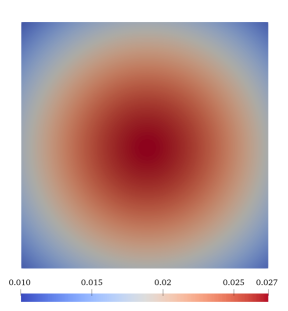
(a)

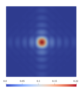
(b)

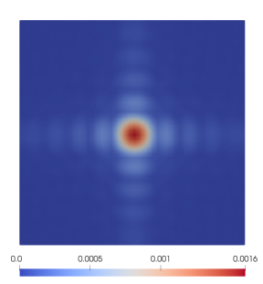
(c)

Figure 1: The absolute value of the simulated data without the noise for the inclusion 1 in Table 1. Here $k=16.2$. see (6.12). a) The measured data $f(\mathbf{x},k)$, b) the propagated data $g_{0}(\mathbf{x},q)$, c) the function $\phi_{0}(\mathbf{x},k)$. Hence, $x,y$ coordinates of inclusion are clearly seen on the propagated data, unlike the measured data. This indicates that the data propagation procedure is quite a useful one.

To propagate the function $f(\mathbf{x},k)$ close to an inclusion, we need to figure out first where this inclusion is located, i.e. we need to estimate the number $\xi$ in (2.1). Fortunately, the data propagation procedure allows us to do this. For example, consider two inclusions with the same size $r=0.3$, but with different dielectric constants $c=3$ and $c=5$. Centers of both are located at the point $\left(0,0,0\right).$ We solve the Lippmann-Schwinger equation for each of these two cases to generate the data at the measurement plane $P_{m}$ with $A=8,$ see (6.11). Next, we propagate the data to several propagated planes $P_{p,a}=\left\{z=a\right\},$ where $a=\left(-8,2\right]$. Here, we use $k=16.2$ (see (6.12)). The dependence of the maximal absolute value of the propagated data $M\left(a\right)=\max_{P_{p,a}}\left|u\left(x,y,a,16.2\right)\right|$ on the number $a$ for these inclusions is depicted in Fig. 2. We see that the function $M\left(a\right)$ attains its maximal value near the point $a_{0}=-0.5$ for both cases. This point is located reasonably close to the actual position of the front faces (at $z=-0.15)$ of the corresponding inclusions. The function $M\left(a\right)$ has attained its maximal value at points $a$ close to $a_{0}$ for all other inclusions we have tested. Therefore, we propagate the measured data for all inclusions to the propagated plane $P_{p,-0.5}=\left\{z=-0.5\right\}$ and we set in (2.1) $\xi=-0.5$.

Figure 2: The depedence of maximum absolute value of propagated data $g(\mathbf{x},k)$ on the locaton of propagation plane $a$ for inclusions with $c=3.0$ (solid line) and $c=5.0$ (dashed line).

We have found in our computations that the optimal interval of wavenumbers is:

$$k\in\left[15.2,16.2\right].$$ (6.12)

We divide this interval in ten (10) subintervals with the step size $\Delta k=0.1.$ For each $k=15.2,15.3,...16.1,16.2$ and for each inclusion under the consideration we solve Lippmann-Schwinger equation (6.10) to generate the function $f(\mathbf{x},k).$ Next, by propagating this data, we obtain the functions $g_{0}(\mathbf{x},k)$ and $g_{1}(\mathbf{x},k)$ in (2.7) and (2.8) respectively. Using (2.4), (3.3), (3.7) and (3.9), consider the function $q(\mathbf{x},k)$ on the propagated plane $P_{p}$, i.e. at the boundary $\Gamma$. In fact, this function is denoted as $\phi_{0}\left(\mathbf{x},k\right)$ in (3.14) and it is one of the two boundary conditions (the second one is $\phi_{1}\left(\mathbf{x},k\right)$ in (3.14)) which generate the function $F_{h}$ in the functional $J_{\lambda,\rho}^{h}\left(p_{h}\right)$ in (6.8). Fig. 1c displays the function $\phi_{0}(\mathbf{x},k)$ for the inclusion number 1 in Table 1 for $k=16.2$.

6.3 Computational domain

To model the experimental setup of [6, 7] we use the following measurement plane:

$$P_{m}=\left\{z=-8\right\},P_{meas}=\{\mathbf{x}:(x,y)\in(-3,3)\times(-3,3),z=-8\},$$

where $P_{meas}\subset P_{m}$ is the square on which measurements are conducted and $z=-8$ corresponds to the 80 cm. The latter is the approximate distance from the center of any inclusion to the plane $\left\{z=0\right\}$ where detectors are located in [6, 7]. Solving equation (6.10), we generate the function $f(\mathbf{x},k),k\in\left[15.2,16.2\right].$ Next, we propagate this function to $\Gamma,$

$$\Gamma=\{\mathbf{x}:(x,y)\in(-3,3)\times(-3,3),z=-0.5\}\subset P_{p}.$$

Here, $z=-0.5$ was found in section 6.2. Finally, we define our computational domain as

$$\Omega=\{\mathbf{x}:(x,y,z)\in(-3,3)\times(-3,3)\times(-0.5,4.5)\}.$$ (6.13)

6.4 Adding noise

We add a random noise to the simulated data $f(\mathbf{x},k)$ as follows:

$$f_{noisy}(\mathbf{x},k)=f(\mathbf{x},k)+\delta\|f(\mathbf{x},k)\|_{L^{2}(\Gamma)}\frac{\sigma(\mathbf{x},k)}{\|\sigma(\mathbf{x},k)\|_{L^{2}(\Gamma)}}.$$

Here, $\delta$ is the noise level. Next, $\sigma(\mathbf{x},k)=\sigma_{1}(\mathbf{x},k)+i\sigma_{2}(\mathbf{x},k)$, where $\sigma_{1}(\mathbf{x},k)$ and $\sigma_{2}(\mathbf{x},k)$ are random numbers uniformly distributed on the interval $(-1,1)$. We use below $\delta=0.15$, i.e. $15\%$ of the additive noise. Fig. 3 displays the absolute value of simulated data with noise $f_{noise}(\mathbf{x},k)$, the corresponding propagated data $g_{0,noisy}(\mathbf{x},k)$ and the function $\phi_{0,noisy}(\mathbf{x},k)$ for the same inclusion and the wavenumber $k=16.2$ as in Fig. 1. We see that the data propagation procedure has a smoothing effect on our noisy measured data, since $g_{0}(\mathbf{x},k)$ in Fig. 1b and $g_{0,noisy}(\mathbf{x},k)$ in Fig. 3b are almost identical.

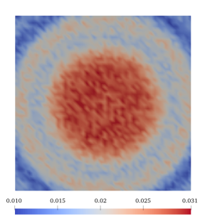
(a)

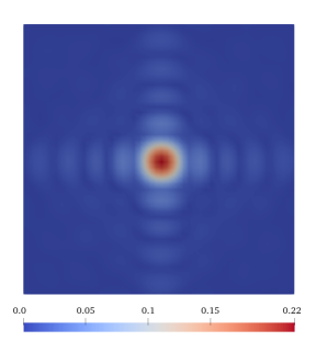
(b)

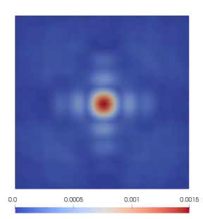
(c)

Figure 3: The absolute value of the computationally simulated data with noise for the inclusion 1 in Table 1. Here $k=16.2$, see (6.12). a) The measured data $f_{noisy}(\mathbf{x},k)$, b) the propagated data $g_{0,noisy}(\mathbf{x},k)$, c) and the function $\phi_{0,noisy}(\mathbf{x},k)$). Comparison of b) with Fig. 1b shows that the data propagation procedure has a significant smoothing effect. Also, just as in Fig. 1, comparison of b) and c) with a) shows that this procedure helps quite significantly to find $x,y$ coordinates of targets of interest.

6.5 The algorithm

Based on the above theory, we use the following algorithm for determining the function $c(\mathbf{x})$ from simulated data with noise $f(\mathbf{x},k)$ (here, the subscript “$noisy$” is left out for convenience, also see item 1 in Remarks 6.1):

1. Using the data propagation procedure, calculate the boundary data $g_{0}(\mathbf{x},k)$ and $g_{1}(\mathbf{x},k)$.

2. Calculate the subsequent boundary conditions $\phi_{0}(\mathbf{x},k)$, $\phi_{1}(\mathbf{x},k)$, $\psi_{0}(\mathbf{x})$, and $\psi_{1}(\mathbf{x})$.

3. Compute the auxiliary functions $Q_{h}(\mathbf{x})$ and $F_{h}(\mathbf{x},k)$.

4. Compute the minimizer $W_{\min,h}(\mathbf{x})$ of the functional $\widetilde{I}_{\mu,\alpha}^{h}\left(W_{h}\right)$ in (6.7).

5. Using the computed function $V_{h}(\mathbf{x})=W_{\min,h}(\mathbf{x})+Q_{h}(\mathbf{x})$, minimize the functional $J_{\lambda,\rho}^{h}(p_{h})$ in (6.8). Let the function $p_{h,\min}(\mathbf{x},k)$ be its minimizer. Calculate the function $q_{h}(\mathbf{x},k)=p_{h,\min}(\mathbf{x},k)+F_{h}(\mathbf{x},k)$.

6. Compute the function $v_{h}(\mathbf{x},k)$ for $k=\underline{k}$ as follows:

   $$v_{h}(\mathbf{x},\underline{k})=-\int_{\underline{k}}^{\overline{k}}q_{h}(\mathbf{x},\kappa)d\kappa+V_{h}(\mathbf{x}).$$

7. Calculate the approximation for the unknown coefficient $c(\mathbf{x})$ using the following formulae, see (2.6), (3.8)

   $$\beta(\mathbf{x})=-\Delta^{h}v_{h}(\mathbf{x},\underline{k})-\underline{k}^{2}\nabla v_{h}(\mathbf{x},\underline{k})\cdot\nabla v(\mathbf{x},\underline{k})+2i\underline{k}v_{z}(\mathbf{x},\underline{k}),$$

   $$c\left(\mathbf{x}\right)=\left\{\begin{array}[]{c}\mathop{\rm Re}\beta\left(\mathbf{x}\right)+1,\text{ if }\mathop{\rm Re}\beta\left(\mathbf{x}\right)\geq 0\text{ and }\mathbf{x}\in\Omega,\\ 1,\text{ otherwise.}\end{array}\right.$$

6.6 Numerical implementation

We now present some details of the numerical implementation. When minimizing functionals $\widetilde{I}_{\mu,\alpha}^{h}\left(W_{h}\right)$ and $J_{\lambda,\rho}^{h}\left(p_{h}\right)$ in (6.7) and (6.8), we use finite differences not only with respect to $x,y$ but with respect to $z$ as well. Thus, $z-$derivatives in these functionals are also written in finite differences. For brevity we use the same notations $\widetilde{I}_{\mu,\alpha}^{h}\left(W_{h}\right)$ and $J_{\lambda,\rho}^{h}\left(p_{h}\right)$ for these functionals.

This is the fully discrete case, unlike the semi-discrete case of (6.7), (6.8). The theory for the fully discrete cases of nonlinear ill-posed problems for PDEs is not yet developed well. It seems that such a theory is much more complicated than the one for the semi-discrete case. There are only a few results for the fully discrete case, and all are for linear ill-posed problems for PDEs, as opposed to our nonlinear case, see, e.g. [56, 57]. Since it is not yet clear to us how to extend above theorems for the fully discrete case, we are not concerned with such extensions here.

We minimize resulting functionals with respect to the values of corresponding functions at grid points. In the computational domain (6.13), we use the uniform grid with $N_{x}=N_{y}=N_{z}=51$ points with the corresponding step sizes $h_{x},h_{y},h_{z}$, where $h_{x}=h_{y}=h.$ The grid point labeled $(j,s,l)$ corresponds to $\mathbf{x}=(x,y,z)=(x_{j},y_{s},z_{l})$. In addition, the interval $k=[\underline{k},\overline{k}]$ of wavenumbers is divided into $N_{k}=11$ points $k_{n}$ with the step size $h_{k}$. Hence, we use the following discrete functions $W_{h}(\mathbf{x})=W(x_{j},y_{s},z_{l})=W_{j,s,l}$ and $p_{h}(\mathbf{x},k)=p_{h}(x_{j},y_{s},z_{l},k_{n})=p_{j,s,l,n}$ at grid points.

To minimize the functionals $\widetilde{I}_{\mu,\alpha}^{h}(W_{j,s,l})$ and $J_{\lambda,\rho}^{h}(p_{j,s,l,n}),$ we use the conjugate gradient method (CG) instead of the gradient projection method, which is suggested by our theory. Indeed, similarly with [1], we have observed that the results obtained by both these methods are practically the same. On the other hand, CG is easier to implement numerically than the gradient projection method. Note that we do not employ the standard line search algorithm for determining the step size of the CG. Instead, we start with the step size $10^{-4}$, which is reduced two times if the value of the corresponding functional on the current iteration exceeds its value on the previous iteration otherwise it remains the same. The minimization algorithm is stopped when the step size is less then $10^{-10}$. We use zero as the starting point of the CG for both functions $W_{j,s,l}$ and $p_{j,s,l,n}$.

Gradients of both functionals $\widetilde{I}_{\mu,\alpha}^{h}(W_{j,s,l})$ and $J_{\lambda,\rho}^{h}(p_{j,s,l,n})$ are calculated analytically on each step, and we do not provide details of this for brevity. Rather, we refer to formulae (7.7) and (7.8) of [58], where gradients of similar functionals are calculated analytically using the Kronecker delta function. Also, due to the difficulty with the numerical implementation of the $H^{2,h}(\Omega_{h})-$norm, we use the simpler $L_{2}$ norm in (6.7). As to (6.8), we have established numerically that the minimization of the functional $J_{\lambda,\rho}^{h}\left(p_{h}\right)$ works better if the regularization term is absent. Hence, we set $\rho=0$ in (6.8).

6.7 Reconstruction results

In this section we present the results of our reconstructions for the inclusions listed in Table 1 using the above algorithm. These results are obtained using the Carleman Weight Function (6.1) with $\mu=8$ in (6.7) and $\lambda=8$ in (6.8). We have found that these are optimal values of the parameters $\mu$ and $\lambda.$ Table 2 lists each inclusion with the maximal value $c_{exact}$ of the exact coefficient $c_{exact}=\max_{inclusion}c\left(\mathbf{x}\right)$, radius $r$, the maximal value of the computed coefficient $c_{comp}=\max_{inclusion}c(\mathbf{x})$, the relative computational error

$$\varepsilon=\frac{|c_{comp}-c_{exact}|}{c_{exact}}\cdot 100\%,$$

and location, i.e. the $z$ coordinate of the point where the value of $c_{comp}$ is achieved.

Note that while we have added $15\%$ noise in our simulated data, the relative computational errors of reconstructed coefficients do not exceed 9% in all cases, which is 1.67 times less than the level of noise in the data. Moreover, the locations of points where the values of $c_{comp}$ are achieved, are reconstructed with a good accuracy as well. Indeed, we need our reconstructed inclusions to be somewhere between $-r$ and $r$, where either $r=0.3$ or $r=0.5$. Fig. 4 displays the exact and computed images for the inclusion number 1 in Table 1. Images are obtained in Paraview.

Until now we have considered only the case of a single inclusion. The case of two inclusions, which is listed as number 4 in Table 1, is very similar. The absolute value of simulated data with noise $f_{noise}(\mathbf{x},k)$, the propagated data $g_{0,noisy}(\mathbf{x},k)$, and the function $\phi_{0,noisy}(\mathbf{x},k)$ for two inclusions and the wavenumber $k=16.2$ are displayed on Fig. 5.

Looking at the original data of Fig. 5a, we cannot clearly distinguish these two inclusions. However, Figures 5b and 5c show that these two inclusions can be clearly separated after the data propagation procedure. Furthermore, these figures also indicate that the left inclusion has a larger dielectric constant and a smaller size than the right one, which is true. The reconstruction results of Fig. 6 reflect this fact too. Here, the locations of both inclusions are computed accurately and the larger inclusion appears larger in the reconstructed image 6b. The values of $c_{comp}$ in both inclusions are also computed with a good accuracy, see Table 2. This result is obtained using the same parameters as in the case with a single inclusion.

Table 2: Reconstruction results

Inclusion number	Exact coef. $c_{exact}$	Radius $r$	Computed coef. $c_{comp}$, error	Location
1	3	0.3	3.17, 5.7%	0.01
2	3	0.5	2.88, 4.0%	0.01
3	5	0.3	5.15, 3.0%	-0.09
4.1	7	0.3	6.36, 9.0%	0.01
4.2	3	0.5	2.99, 0.3%	0.01

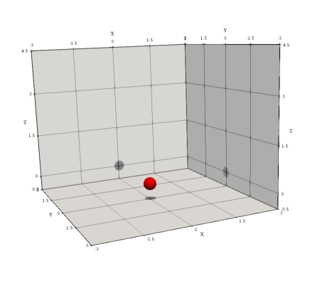
(a)

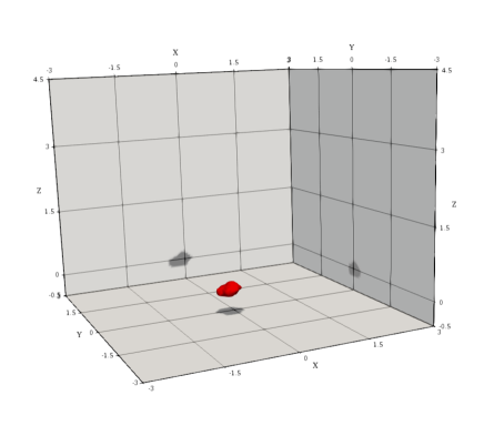
(b)

Figure 4: Reconstruction result for the inclusion number 1: exact image (a) and computed image (b)

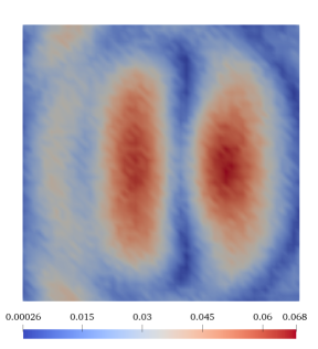
(a)

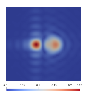
(b)

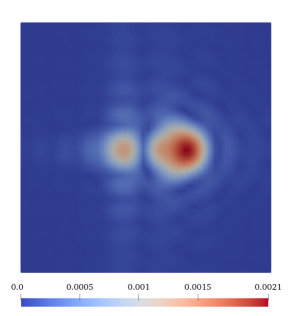
(c)

Figure 5: The absolute value of the simulated data with 15% noise for the case of two inclusions listed as number 4 in Table 1. Here $k=16.2.$ a) The measured data $f_{noisy}\left(\mathbf{x},k\right),$ b) the propagated data $g_{0,noisy}\left(\mathbf{x},k\right),$ c) the function $\phi_{0,noisy}.$ Observe that the data propagation procedure helps to separate these two inclusions. Also, it is clear from b), c) that the left inclusion has a larger dielectric constant and a smaller size than the right inclusion.

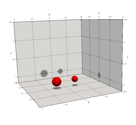
(a)

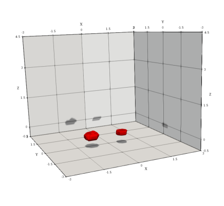
(b)

Figure 6: Reconstruction result for two inclusions: exact image (a) and computed image (b)

References

- [1] M. V. Klibanov, A. E. Kolesov, L. Nguyen, A. Sullivan, Globally strictly convex cost functional for a 1-D inverse medium scattering problem with experimental data, SIAM J. on Applied Mathematics 77 (5) (2017) 1733–1755.
- [2] L. Beilina, M. V. Klibanov, A globally convergent numerical method for a coefficient inverse problem, SIAM Journal on Scientific Computing 31 (1) (2008) 478–509.
- [3] L. Beilina, M. V. Klibanov, Approximate Global Convergence and Adaptivity for Coefficient Inverse Problems, Springer, 2012.
- [4] M. V. Klibanov, D.-L. Nguyen, L. H. Nguyen, H. Liu, A globally convergent numerical method for a 3D coefficient inverse problem with a single measurement of multi-frequency data, accepted for publication in Inverse Problems and Imaging, also available in arXiv: 1612.0414.
- [5] A. E. Kolesov, M. V. Klibanov, L. H. Nguyen, D.-L. Nguyen, N. T. Thanh, Single measurement experimental data for an inverse medium problem inverted by a multi-frequency globally convergent numerical method, Applied Numerical Mathematics 120 (2017) 176–196.
- [6] D.-L. Nguyen, M. V. Klibanov, L. H. Nguyen, M. A. Fiddy, Imaging of buried objects from multi-frequency experimental data using a globally convergent inversion method, J. Inverse and Ill-Posed Problems, accepted for publication (2017), available online, DOI: 10.1515/jiip-2017- 0047.
- [7] D.-L. Nguyen, M. V. Klibanov, L. H. Nguyen, A. E. Kolesov, M. A. Fiddy, H. Liu, Numerical solution of a coefficient inverse problem with multi-frequency experimental raw data by a globally convergent algorithm, Journal of Computational Physics 345 (2017) 17–32.
- [8] L. Beilina, M. V. Klibanov, Globally strongly convex cost functional for a coefficient inverse problem, Nonlinear Analysis: Real World Applications 22 (2015) 272–288.
- [9] M. V. Klibanov, O. V. Ioussoupova, Uniform strict convexity of a cost functional for three-dimensional inverse scattering problem, SIAM Journal on Mathematical Analysis 26 (1) (1995) 147–179.
- [10] M. V. Klibanov, Global convexity in a three-dimensional inverse acoustic Problem, SIAM Journal on Mathematical Analysis 28 (6) (1997) 1371–1388.
- [11] M. V. Klibanov, Global convexity in diffusion tomography, Nonlinear World 4 (1997) 247–265.
- [12] M. V. Klibanov, A. Timonov, Carleman Estimates for Coefficient Inverse Problems and Numerical Applications, de Gruyter, Utrecht, 2004.
- [13] M. V. Klibanov, V. G. Kamburg, Globally strictly convex cost functional for an inverse parabolic problem, Mathematical Methods in the Applied Sciences 39 (4) (2016) 930–940.
- [14] M. V. Klibanov, L. H. Nguyen, A. Sullivan, L. Nguyen, A globally convergent numerical method for a 1-d inverse medium problem with experimental data, Inverse Problems and Imaging 10 (4) (2016) 1057–1085.
- [15] M. V. Klibanov, N. T. Thành, Recovering dielectric constants of explosives via a globally strictly convex cost functional, SIAM Journal on Applied Mathematics 75 (2) (2015) 518–537.
- [16] G. Chavent, Nonlinear Least Squares for Inverse Problems - Theoretical Foundations and Step-by-Step Guide for Applications, Springer, 2009.
- [17] A. Goncharsky, S. Romanov, Supercomputer technologies in inverse problems of ultrasound tomography, Inverse Problems 29 (2013) 075004.
- [18] A. V. Goncharsky, S. Y. Romanov, Iterative methods for solving coefficient inverse problems of wave tomography in models with attenuation, Inverse Problems 33 (2) (2017) 025003.
- [19] J. A. Scales, M. L. Smith, T. L. Fischer, Global optimization methods for multimodal inverse problems, Journal of Computational Physics 103 (2) (1992) 258–268.
- [20] A. Lakhal, KAIRUAIN-algorithm applied on electromagnetic imaging, Inverse Problems 29 (2010) 095001.
- [21] A. Lakhal, A direct method for nonlinear ill-posed problems, Inverse Problems, accepted for publication, available online at http://iopscience.iop.org/article/10.1088/1361-6420/aa91e0/pdf.
- [22] M. V. Klibanov, N. A. Koshev, J. Li, A. G. Yagola, Numerical solution of an ill-posed Cauchy problem for a quasilinear parabolic equation using a Carleman weight function, Journal of Inverse and Ill-posed Problems 24 (2016) 761–776.
- [23] A. B. Bakushinskii, M. V. Klibanov, N. A. Koshev, Carleman weight functions for a globally convergent numerical method for ill-posed Cauchy problems for some quasilinear PDEs, Nonlinear Analysis: Real World Applications 34 (2017) 201–224.
- [24] M. V. Klibanov, Carleman weight functions for solving ill-posed Cauchy problems for quasilinear PDEs, Inverse Problems 31 (12) (2015) 125007.
- [25] A. Bukhgeim, M. Klibanov, Uniqueness in the large of a class of multidimensional inverse problems, Soviet Math. Doklady 17 (1981) 244–247.
- [26] M. V. Klibanov, Carleman estimates for global uniqueness, stability and numerical methods for coefficient inverse problems, Journal of Inverse and Ill-Posed Problems 21 (4) (2013) 477–560.
- [27] L. Baudouin, M. d. Buhan, S. Ervedoza, Convergent algorithm based on Carleman estimates for the recovert of a potential in the wave equation, SIAM J. on Numerical Analysis 55 (2017) 1578–1613.
- [28] H. Ammari, J. Garnier, W. Jing, H. Kang, M. Lim, K. Solna, H. Wang, Mathematical and statistical methods for multistatic imaging, Lecture Notes in Mathematics 2098 (2013) 125–157.
- [29] H. Ammari, Y. Chow, J. Zou, The concept of heterogeneous scattering and its applications in inverse medium scattering, SIAM J. Mathematical Analysis 46 (2014) 2905–2935.
- [30] H. Ammari, Y. Chow, J. Zou, Phased and phaseless domain reconstruction in inverse scattering problem via scattering coefficients, SIAM J. Applied Mathematics 76 (2016) 1000–1030.
- [31] G. Bao, P. Li, J. Lin, F. Triki, Inverse scattering problems with multi-frequencies, Inverse Problems 31 (2015) 093001.
- [32] M. de Buhan, M. Kray, A new approach to solve the inverse scattering problem for waves: combining the TRAC and the Adaptive Inversion methods, Inverse Problems 29 (2013) 085009.
- [33] Y. T. Chow, J. Zou, A numerical method for reconstructing the coefficient in a wave equation, Numerical Methods in Partial Differential Equations 31 (2015) 289–307.
- [34] Y. T. Chow, K. Ito, K. Liu, J. Zou, Direct sampling method in diffuse optical tomography, SIAM J. Scientific Computing 37 (2015) A1658–A1684.
- [35] K. Ito, B. Jin, J. Zou, A direct sampling method for inverse electromagnetic medium scattering, Inverse Problems 29 (9) (2013) 095018.
- [36] B. Jin, Z. Zhou, A finite element method with singularity reconstruction for fractional boundary value problems, ESAIM: Mathematical Modelling and Numerical Analysis 49 (2015) 1261–1283.
- [37] S. Kabanikhin, A. Satybaev, M. Shishlenin, Direct Methods of Solving Multidimensional Inverse Hyperbolic Problem, VSP, 2004.
- [38] S. Kabanikhin, K. Sabelfeld, N. Novikov, M. Shishlenin, Numerical solution of the multidimensional Gelfand-Levitan equation, J. Inverse and Ill-Posed Problems 23 (2015) 439–450.
- [39] S. Kabanikhin, N. Novikov, I. Osedelets, M. Shishlenin, Fast Toeplitz linear system inversion for solving two-dimensional acoustic inverse problem, J. Inverse and Ill-Posed Problems 23 (2015) 687–700.
- [40] A. Lakhal, A decoupling-based imaging method for inverse medium scattering for Maxwell’s equations, Inverse Problems 26 (2010) 015007.
- [41] J. Li, H. Liu, Q. Wang, Enhanced multilevel linear sampling methods for inverse scattering problems, J. Comput. Phys. 257 (2014) 554–571.
- [42] J. Li, P. Li, H. Liu, X. Liu, Recovering multiscale buried anomalies in a two-layered medium, Inverse Problems 31 (2015) 105006.
- [43] H. Liu, Y. Wang, C. Yang, Mathematical design of a novel gesture-based instruction/input device using wave detection, SIAM J. Imaging Sci. 9 (2016) 822–841.
- [44] M. V. Klibanov, D.-L. Nguyen, L. H. Nguyen, A coefficient inverse problem with a single measurement of phaseless scattering data, arXiv:1710.04804.
- [45] M. V. Klibanov, V. Romanov, Two reconstruction procedures for a 3-D phaseless inverse scattering problem for the generalized Helmholtz equation, Inverse Problems 32 (2016) 0150058.
- [46] V. Romanov, Inverse Problems of Mathematical Physics, VNU Science Press, 1987.
- [47] D. Gilbarg, N. Trudinger, Elliptic Partial Differential Equations of Second Order, Springer, 1984.
- [48] V. Romanov, Inverse problems for differential equations with memory, Eurasian J. of Mathematical and Computer Applications 2 (4) (2014) 51–80.
- [49] M. V. Klibanov, Carleman estimates for the regularization of ill-posed Cauchy problems, Applied Numerical Mathematics 94 (2015) 46–74.
- [50] A. Tikhonov, A. Goncharsky, V. Stepanov, A. Yagola, Numerical Methods for the Solution of Ill-Posed Problems, Kluwer, London, 1995.
- [51] N. T. Thành, L. Beilina, M. V. Klibanov, M. A. Fiddy, Imaging of buried objects from experimental backscattering time-dependent measurements using a globally convergent inverse algorithm, SIAM Journal on Imaging Sciences 8 (1) (2015) 757–786.
- [52] G. Vainikko, Fast solvers of the Lippmann-Schwinger equation, in: D. Newark (Ed.), Direct and Inverse Problems of Mathematical Physics, Int. Soc. Anal. Appl. Comput. 5, Kluwer, Dordrecht, 2000, p. 423.
- [53] A. Lechleiter, D.-L. Nguyen, A trigonometric Galerkin method for volume integral equations arising in TM grating scattering, Advanced Computational Mathematics 40 (2014) 1–25.
- [54] https://en.wikipedia.org/wiki/M14_mine.
- [55] L. Novotny, B. Hecht, Principles of Nano-Optics, 2nd Edition, Cambridge University Press, Cambridge, 2012.
- [56] E. Burman, J. Ish-Horowicz, L. Oksanen, Fully discrete finite element data assimilation method for the heat equation, arXiv:1707.06908.
- [57] M. Klibanov, F. Santosa, A computational quasi-reversibility method for Cauchy problems for Laplace’s equation, SIAM J. Applied Mathematics 51 (1991) 1653–1675.
- [58] A. V. Kuzhuget, M. Klibanov, Global convergence for a 1-D inverse problem with application to imaging of land mines, Applicable Analysis 89 (2010) 125–157.