Transport coefficients in the Polyakov quark meson coupling model: A quasi particle approach

Abstract

We compute the transport coefficients, namely, the coefficients of shear and bulk viscosities as well as thermal conductivity for hot and dense matter. The calculations are performed within the Polyakov loop extended quark meson model. The estimation of the transport coefficients is made using the Boltzmann kinetic equation within the relaxation time approximation. The energy dependent relaxation time is estimated from meson meson scattering, quark meson scattering and quark quark scattering within the model. In our calculations, the shear viscosity to entropy ratio and the coefficient of thermal conductivity show a minimum at the critical temperature, while the ratio of bulk viscosity to entropy density exhibits a peak at this transition point. The effect of confinement modelled through a Polyakov loop potential plays an important role in the estimation of these dissipative coefficients both below and above the critical temperature.

(To appear in Proceedings of Science, Proceedings of ”Critical Point and Onset of Deconfinement - CPOD2017 7-11 August, 2017 The Wang Center, Stony Brook University, Stony Brook, NY)

I Introduction

Transport coefficients of matter under extreme conditions of temperature, density or external fields are interesting and important for several reasons. In the context of relativistic heavy ion collisions, these properties enter as dissipative coefficients in the hydrodynamic evolution of the quark gluon plasma. They are also important for the cooling of neutron stars. The cooling of neutron stars at short time scales constrains the thermal conductivity chamel while the cooling through neutrino emission on a much larger time scales constrains the phase of the matter in the interior of the compact star yakovlev . Apart from these, the temperature and chemical potential dependence of the transport coefficients may actually reveal the location of phase transitions kapustabk .

Transport coefficients for QCD matter in principle can be calculated using Kubo formulation kubo . However, QCD is strongly interacting for both at energies accessible in heavy ion collision experiments as well as for the densities expected to be there in the core of the neutron stars making the perturbative estimations unreliable. Calculations using lattice QCD simulations at finite chemical potential is also challenging and is limited only to the equilibrium thermodynamic properties at small chemical potentials. This has motivated to estimate the transport coefficient in various effective models of strong interaction physics. These include chiral perturbation theory dobadoch , quasi-particle models quasip , linear sigma model purnendu and the Nambu- Jona-Lasinio model sasakinjl ; deb . The general temperature dependence of the viscosity coefficients turns out to be similar with the ratio of shear viscosity to entropy density ($\eta/s$) exhibiting a minimum at the transition temperature. The numerical value of $\eta$ at the minimum however differ by order of magnitude. Similarly, the bulk viscosity shows a maximum near the critical temperature. The numerical values of these coefficients however, vary over a large range of values e.g. $\zeta$ varies from $10^{-5}$ GeV³ souravsuk to $10^{-2}$ GeV³ around the critical temperature sasakinjl .

The other transport coefficient that is important at finite baryon density is the coefficient of thermal conductivity $\lambda$ denicolhydro ; denicolpre ; denicolheat . This coefficient has been evaluated in various effective models like Nambu Jona Lasinio model using Green-Kubo approach fukutome , relaxation time approximation deb and the instanton liquid model nam . The results, however, vary over a wide range of values, with $\lambda=0.008$ GeV^-2 as in Ref. nicola to $\lambda\sim 10$ GeV^-2 as in Ref. marty for a range of temperatures (0.12 GeV $<$T$<$ 0.17 GeV), which has been nicely tabulated in Ref. sabyath .

We shall here attempt to estimate these transport coefficients within an effective model of strong interaction, the Polyakov loop extended quark meson (PQM) model that incorporates the aspects of chiral symmetry breaking in strong interaction and takes care of confinement deconfinement transition partially while explicitly keeping pionic degrees of freedom at low temperature.

The transport coefficients are evaluated within the relaxation time approximation of Boltzmann equation which is a reasonable approximation for quasi particles quasip ; guru . The relaxation time is calculated from the scattering of the particles that constitute the dynamical degrees of freedom of the model - namely the meson scattering, as is considered in Ref.purnendu with medium dependent meson masses; quark scattering through meson exchanges similar to as considered in Ref.s sasakinjl ; deb ; marty with medium dependent quark and meson masses and quark meson scattering. As we shall see in the following, each of these processes bring out distinct features for the transport coefficients.

II Thermodynamics of PQM model

The thermodynamic potential in PQM model is given bybjschaefer ; bielich ; buballa ; ranjita

$$\Omega(T,\mu)=\Omega_{\bar{q}q}+U_{\chi}+U_{P}(\phi,\bar{\phi})$$ (1)

The fermionic (quark) part of the thermodynamic potential is given as

$$\Omega_{\bar{q}q} = -2N_{f}T\int\frac{d^{3}p}{(2\pi)^{3}}\bigg{[}\ln\left(1+3(\phi+\bar{\phi}e^{-\beta\omega_{-}})e^{-\beta\omega_{-}}+e^{-3\beta\omega_{-}}\right)$$ (2)

$$+ \ln\left(1+3(\bar{\phi}+\phi e^{-\beta\omega_{+}})e^{-\beta\omega_{+}}+e^{-3\beta\omega_{+}}\right)\bigg{]}$$

modulo a divergent vacuum part. In the above, $\omega_{\mp}=E_{p}\mp\mu$, with the single particle quark/anti-quark energy $E_{p}=\sqrt{{\bf{p}}^{2}+M^{2}}$. The constituent quark/anti-quark mass is defined to be

$$M^{2}=g_{\sigma}^{2}(\sigma^{2}+{\bf{\pi}}^{2}).$$ (3)

In Eq.(1), potential $U_{\chi}(\sigma,{\bf{\pi}})$ is the mesonic potential that essentially describes the chiral symmetry breaking pattern in strong interaction and is given by

$$U_{\chi}(\sigma,\mbox{\boldmath$\pi$})=\frac{\lambda}{4}(\sigma^{2}+\mbox{\boldmath$\pi$}^{2}-v^{2})-c\sigma$$ (4)

while, the last term in Eq.(1) is the Polyakov loop potential that essentially describes the confinement deconfinement transition. polynomial parametrization bjschaefer

$$U_{P}(\phi,\bar{\phi})=T^{4}\left[-\frac{b_{2}(T)}{2}\bar{\phi}\phi-\frac{b_{3}}{2}(\phi^{3}+\bar{\phi}^{3})+\frac{b_{4}}{4}(\bar{\phi}\phi)^{2}\right],$$ (5)

with the temperature dependent coefficient $b_{2}$ given as

$$b_{2}(T)=a_{0}+a_{1}(\frac{T_{0}}{T})+a_{2}(\frac{T_{0}}{T})^{2}+a_{3}(\frac{T_{0}}{T})^{3}$$ (6)

The numerical values of the parameters are $a_{0}=6.75,a_{1}=-1.95,a_{2}=2.625,a_{3}=-7.44,b_{3}=0.75,b_{4}=7.5$ The parameter $T_{0}$ corresponds to the transition temperature of Yang-Mills theory. However, for the full dynamical QCD, there is a flavor dependence on $T_{0}(N_{f})$. For two flavors we take it to be $T_{0}(2)=192$ MeV as in Ref.bjschaefer . The parameters of potential $U_{\chi}$,are so chosen that the chiral symmetry is broken spontaneously in vacuum with $\langle\sigma\rangle=f_{\pi}$, and $\langle\mbox{\boldmath$\pi$}\rangle=0$ with $f_{\pi}=93$MeV is the pion decay constant. The coefficient of symmetry breaking term is fixed from PCAC so that $c=f_{\pi}^{2}m_{\pi}^{2}$; $v^{2}=f_{\pi}^{2}-m_{\pi}^{2}/\lambda$, with $\lambda$ determined from mass of the $\sigma$ meson leading to $\lambda=19.7$ and $g_{\sigma}=3.3$ so that the constituent quark mass in the vacuum is about 300 MeVrischkeqm . The mean fields are obtained by minimizing $\Omega$ with respect to $\sigma$, $\phi$, $\bar{\phi}$, and $\pi$. For example, extremising the effective potential with respect to $\sigma$ field leads to

$$\lambda(\sigma^{2}+{\bf{\pi}}^{2}-v^{2})-c+g_{\sigma}\rho_{s}=0$$ (7)

where, the scalar density $\rho_{s}=-\langle\bar{\psi}\psi\rangle$ is given by

$$\rho_{s}=6N_{f}g_{\sigma}\sigma\int\frac{d{\bf{p}}}{(2\pi)^{3}}\frac{1}{E_{P}}\left[f_{-}({\bf{p}})+f_{+}({\bf{p}})\right].$$ (8)

In the above, $f_{\mp}({\bf{p}})$ are the distribution functions for the quarks and anti-quarks, with $\omega_{\mp}=E({\bf{p}})\mp\mu$, given as

$$f_{-}({\bf{p}})=\frac{\phi e^{-\beta\omega_{-}}+2\bar{\phi}e^{-2\beta\omega_{-}}+e^{-3\beta\omega_{-}}}{1+3\phi e^{-\beta\omega_{-}}+3\bar{\phi}e^{-2\beta\omega_{-}}+e^{-3\beta\omega_{-}}},$$ (9)

and,

$$f_{+}({\bf{p}})=\frac{\bar{\phi}e^{-\beta\omega_{+}}+2\phi e^{-2\beta\omega_{+}}+e^{-3\beta\omega_{+}}}{1+3\bar{\phi}e^{-\beta\omega_{+}}+3\phi e^{-2\beta\omega_{+}}+e^{-3\beta\omega_{+}}}.$$ (10)

It can be shown that for vanishing chemical potential, $\phi=\bar{\phi}$ and the distribution functions become

$$f_{\phi}({\bf{p}})=\frac{\phi e^{-\beta E_{-}}+2\phi e^{-2\beta E}+e^{-3\beta E}}{1+3\phi e^{-\beta E}+3\phi e^{-2\beta E}+e^{-3\beta E}},$$ (11)

where, $E({\bf{p}})$ is the single particle energy for the quarks.

The meson masses for $\sigma$ and $\pi$ are determined by the curvature of $\Omega$ at the global minimum

$$M_{\sigma}^{2}=\frac{\partial^{2}\Omega}{\partial\sigma^{2}}|_{\sigma=\sigma_{0},\pi=0},\quad\quad M_{\pi_{i}}^{2}=\frac{\partial^{2}\Omega}{\partial\pi_{i}^{2}|_{\sigma=\sigma_{0},\pi=0}}.$$ (12)

The energy density $\epsilon=\Omega-T\partial\Omega/\partial T+\mu\rho_{q}$ is given by

$$\epsilon=\frac{6}{\pi^{2}}\int p^{2}dpE({\bf{p}})\left(f_{-}({\bf{p}})+f_{+}({\bf{p}})\right)+U_{\chi}-3U_{P}(\phi,\bar{\phi})+\frac{T^{5}}{2}\frac{db_{2}(T)}{dT}\bar{\phi}\phi$$ (13)

In Fig.1(a), we have plotted the constituent quark mass, and the meson masses in the model as a function of temperature for vanishing baryon density. In the chirally broken phase, m_π, being the mass of an approximate Goldstone mode is protected and varies weakly with temperature. On the other hand, the mass of $\sigma$ , $M_{\sigma}$, which is approximately twice the constituent quark mass,$M$ drops significantly near the crossover temperature. At high temperature, being chiral partners, the masses of $\sigma$ and $\pi$ mesons become degenerate and increase linearly with temperature. In Fig. 1b, we have plotted the order parameters $\sigma$ and $\phi$ as a function of temperature for vanishing quark chemical potential. We also note that for $\mu=0$, the order parameters $\phi$ and $\bar{\phi}$ are the same. Because of the approximate chiral symmetry, the chiral order parameter decreases with temperatures to small values but never vanishes. The Polyakov loop parameter on the other hand grows from $\phi=0$ at zero temperature to about $\phi=1$ at high temperatures. We might mention here that at very high temperature exceeds unity, the value in the infinite quark mass limit.

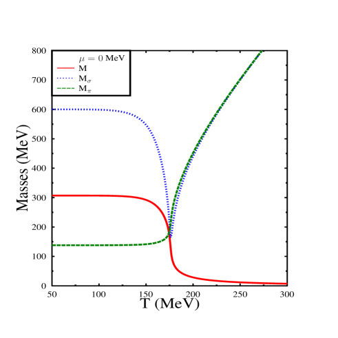
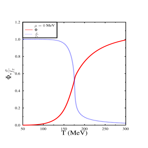
Fig. 1-a	Fig. 1-b

Figure 1: (Fig 1 a) Temperature dependence of the masses of constituent quarks ($M$), and pions ($M_{\pi}$) and sigma mesons ($M_{\sigma}$) and (Fig1-b) the order parameters $\sigma$ and $\phi$ as a function of temperature for $\mu=0$ MeV .

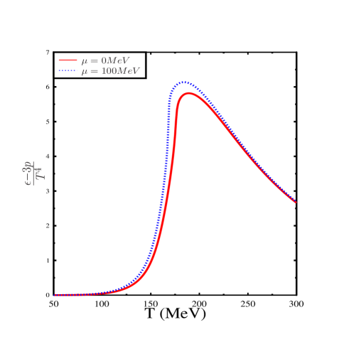
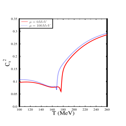
Fig. 2-a	Fig. 2-b

Figure 2: (Fig 2 a)Temperature dependence of the scaled trace anomaly $\frac{\epsilon-3p}{T^{4}}$ and (Fig2 b)Temperature dependence of the velocity of sound at constant density.

Next, in Fig 2a, we show the dependence of the trace anomaly $(\epsilon-3p)/T^{4}$ on temperature. The conformal symmetry is broken maximally at the critical temperature. Further finite chemical potential enhances this breaking as it breaks scale symmetry explicitly. As we shall see later this will have its implication on the bulk viscosity coefficient.

The other thermodynamic quantity that enters into the transport coefficient calculation is the velocity of sound. The same at constant density is defined as

$$c_{s}^{2}=\left(-\frac{\partial P}{\partial\epsilon}\right)_{n}=\frac{s\chi_{\mu\mu}-\rho\chi_{\mu T}}{T(\chi_{TT}\chi_{\mu\mu}-\chi_{\mu T}^{2})}$$ (14)

where, $P$,the pressure, is the negative of the thermodynamic potential given in Eq.(1). Further, $s=-\frac{\partial\Omega}{\partial T}$ is the entropy density and the susceptibilities are defined as $\chi_{xy}=-\frac{\partial^{2}\Omega}{\partial x\partial y}$. This is plotted in Fig. 2b. The velocity of sound shows a minimum near the crossover temperature. Within the model, at low temperature when the constituent quarks start contributing to the pressure, their contribution to the energy density is significant compared to their contribution to the pressure leading to decreasing behavior of velocity of sound till the crossover temperature beyond which it increases as the quarks become light and approach the massless limit of $c_{s}^{2}=\frac{1}{3}$. Such a dip in the velocity of sound is also observed in lattice simulation tanmoy . As we shall observe later this behavior will have important consequences for the behavior of bulk viscosity as a function of temperature. We might mention here that such a dip for the sound velocity was not observed for two flavor NJL deb . For in the linear sigma model calculations such a dip was observed only for a large sigma meson masspurnendu .

III Transport coefficients in relaxation time approximation

Within a quasi-particle approach, a kinetic theory treatment for estimation of transport coefficients can be a reasonable approximation quasip . To solve the relativistic Boltzmann equation, we shall further use the relaxation time approximation where the particle masses are medium dependent. Such attempts were made earlier for $\sigma$-modelpurnendu as well as NJL model to compute the shear and bulk viscosity coefficients. Such an approach was also made to estimate the viscosity coefficients of pure gluon matterquasip . The expressions for the viscosity coefficients were put on a firmer ground by deriving the expressions when there are mean fields and medium dependent masses in a quasi particle picture albright . The resulting expressions for the transport coefficients were manifestly positive definite as they should be. These expressions were derived explicitly for NJL model in Ref.deb . However, a direct generalization of the expressions for the transport coefficients in presence of background gluon fields is not straight forward. The reason being the equilibrium distribution functions for the quarks and antiquarks as given in Eq.s (9) and (10) are not Fermi distribution function. To make the discussion simpler let us consider the case of vanishing baryon chemical potential which we discuss in the following.

Let us first note that the background gluon field couple to quarks through covariant derivative as $D_{\mu}=\partial_{\mu}-\delta_{\mu 0}A_{0}$. In the Polyakov gauge, the Wilson line is $L$ is in the diagonal representation in the color space and therefore, the background gluon field act as an imaginary chemical potential for the colored particles. The corresponding color dependent equilibrium distribution function for the quarks and the anti-quarks are given by pisarskijhep

$$f_{i}(E)=\frac{1}{e^{\beta(E-iQ_{i})}+1};\quad\bar{f}_{i}(E)=\frac{1}{e^{\beta(E+iQ_{i})}+1}$$ (15)

where, we have written $A_{0}^{ij}=\frac{1}{g}\delta^{ij}Q^{i}$, without any summation over the index $i$. As $A_{0}$ is traceless, $\sum_{i}Q^{i}=0$. The Polyakov loop $\phi$ is thus related to $Q_{i}$ as $\phi=\frac{1}{3}\sum_{i}e^{i\beta Q_{i}}$. Further, for vanishing baryon density, one can choose $\phi$ to be real and parameterize $Q^{i}=2\pi T(-q,0,q)$ with $q$ as the dimension less condensate variable. The Polyakov loop variable $\Phi$ is therefore given by

$$\phi=\frac{1}{3}(1+2\cos{2\pi q}).$$ (16)

It is easy to check that the the distribution function of Eq.(9) is the color averaged distribution function .i.e $f_{\phi}(E)=\frac{1}{3}\sum_{i}f_{i}(E)$.

One can write down a Boltzmann kinetic equation for the color dependent the single particle distribution function $\phi_{i}$ of Eq.(15) as

$$\frac{df_{ia}}{dt}=\frac{P^{\mu}}{E_{a}}\partial_{\mu}f^{ia}-\frac{M}{E_{a}}\frac{\partial M}{\partial x^{i}}\frac{\partial f_{ia}}{\partial p^{i}}=-C^{ai}(f_{ia}).$$ (17)

To estimate the transport coefficient, one is interested in small departure from equilibrium and one writes f_ia=f${}_{ia}^{0}$+f${}_{ia}^{1}$, where f${}_{ia}^{0}$ is the equilibrium distribution function, f${}_{ia}^{0}=[exp(\beta)u_{\nu}({\bf{x}})\mp i\beta Q_{i}({\bf{x}})]^{-1}.$ Within the relaxation time approximation, in the collision term, all the distribution functions are given by the equilibrium distribution function except for $f_{ia}$. The collision term then, upto first order in deviation from the equilibrium distribution function, will be proportional to $f^{1}_{ia}$ as $C(f_{ia}^{0})=0$ by local detailed balance. The collision term is then given by

$$C(f_{ia})=-\frac{f^{1}_{ia}}{\tau_{ia}}.$$ (18)

where, $\tau_{ia}$ is the color dependent relaxation time and is in general a function of energy. One can follow he same procedure as in Ref.albright ; deb to calculate e.g. the shear viscosity coefficient $\eta$ and the expression for the same is given by

$$\eta=\frac{1}{45T}\sum_{i,a}\int\frac{d{\bf{p}}}{(2\pi)^{3}}\frac{p_{a}^{4}}{E_{a}^{2}}\tau_{i,a}(E_{a})f_{ia}^{0}(1-f_{i,a}^{0})$$ (19)

In the following we shall replace $\tau_{i,a}(E_{a})$ by its color averaged relaxation time $\tau_{a}(E_{a})$ which for $N_{c}$=3 is given as

$$\tau_{a}^{-1}=\frac{1}{3}\sum_{i}\tau_{ia}(E_{a})=\frac{1}{3}\sum_{i,j,k,l}\int d\Gamma^{b}d\Gamma^{c}d\Gamma^{d}W_{ia,jb\to kc,ld}\left[f_{jb}^{0}(1-f_{kc}^{0})(1-f_{ld}^{0})\right]$$ (20)

where, $d\Gamma_{a}=\frac{d{\bf{p}}_{a}}{(2\pi)^{3}2E_{a}}$, and,

$$W_{ia,jb\to kc,ld}=(2\pi)^{4}\delta^{4}(p_{a}+p_{b}-p_{c}-p_{d})|M_{ia,jb\to kc,ld}|^{2}$$ (21)

with $|M|^{2}$ being the corresponding square of the matrix element for the scattering process. Now, within the model, since we do not have dynamical gluons and we consider scattering through meson exchanges, the interactions are are color preserving and, $W_{ia,jb\to kc,ld}\propto\delta{ik}\delta{jl}$ so that,

$$\tau_{a}^{-1}(E_{a})=\frac{1}{3}\sum_{i,j}\int d\Gamma^{b}d\Gamma^{c}d\Gamma^{d}W_{ia,jb\to ic,jd}\left[f_{jb}^{0}(1-f_{ic}^{0})(1-f_{jd}^{0})\right]$$ (22)

The color sum of the distribution functions become

$${\cal F}(E_{a},E_{c}) \equiv \sum_{i}f_{i}^{0}(E_{a})(1-f_{i}^{0}(E_{c}))=3f_{\phi}-\frac{1}{D(E_{a})D(E_{c})}\bigg{[}3e^{-3\beta(E_{a}+E_{c})}+3\phi(3\phi-2)e^{-\beta(E_{a}+E_{c})}$$ (23)

$$+ 3\phi\left(e^{-\beta(E_{a}+3E_{c})}+e^{-\beta(E_{c}+3E_{a})}\right)+6\phi^{-2\beta(E_{a}+E_{c})}$$

$$+ 3\phi(3\phi-1)\left(e^{-\beta(E_{a}+2E_{c})}+e^{-\beta(E_{c}+2E_{a})}\right)\bigg{]},$$

where, $D(E)$ is the denominator of the Polyakov loop distribution function Eq.(11), $D(E)=1+3\phi e^{-\beta E}+3\phi e^{-2\beta E}+3e^{-3\beta E}$. Eq.(22) then reduces to

$$\tau_{a}^{-1}(E_{a})=\int d\Gamma^{b}d\Gamma^{c}d\Gamma^{d}W_{ia,jb\to ic,jd}(1-f_{\phi}^{0c}){\cal F}(E_{b},E_{d})$$ (24)

The expression for $\eta$, Eq.(19) using Eq.(23), becomes

$$\eta=\frac{1}{45T}\sum_{a}\int\frac{d{\bf{p}}}{(2\pi)^{3}}\frac{p_{a}^{4}}{E_{a}^{2}}\tau_{a}(E_{a}){\cal F}(E_{a},E_{a})$$ (25)

One can further approximate the expression for $\eta$ by replacing the distribution functions in Eq.(19) or equivalently in Eq.(23) by their color averaged value so that $\eta$ reduces to more familiar expression as $\eta$ becomes

$$\eta=\frac{1}{15T}\sum_{a}\int\frac{d{\bf{p}}}{(2\pi)^{3}}\frac{p_{a}^{4}}{E_{a}^{2}}\tau(E_{a})f_{a}^{0}(1\pm f_{a}^{0})$$ (26)

where, the sum is over all the different species contributing to the viscosity coefficients including the antiparticles, and, $\tau^{a}$ is the energy dependent relaxation time given in Eq.(20) which we shall estimate in the following subsection. Let us note that while such a replacement of the color averaged distribution function is exact in the Boltzmann limit, the leading term for difference between replacing the colored distribution function and their color averaged one in the expression $\sum_{i}f_{ia}(1-f_{ia})$ is proportional to $\phi(\phi-1)e^{-2\beta E}$. This difference is small both below and above the critical temperature while it can be relevant around the critical temperature. We have verified numerically that such a difference does not change the quantitative values for the transport coefficients except near the critical temperature.

The coefficient of bulk viscosity is given by

$$\zeta = \frac{1}{27T}\sum_{a}\int\frac{d{\bf{p}}}{(2\pi)^{3}}\frac{\tau^{a}}{E_{a}{}^{2}}{\cal F}(E_{a},E_{a})\bigg{[}{\bf{p}}^{2}\left(1-3v_{n}{}^{2}\right)-3v_{n}{}^{2}\left(M^{2}-TM\frac{dM}{dT}-{\mu M}\frac{{dM}}{d\mu}\right)$$ (27)

$$+ 3\left(\frac{\partial P}{\partial n}\right)_{\epsilon}\left(M\frac{dM}{d\mu}-E_{a}t^{a}\right)\bigg{]}^{2}$$

The thermal conductivity on the other hand is given by

$$\lambda=\frac{1}{3}\left(\frac{w}{nT}\right)^{2}\sum_{a}\int\frac{d{\bf{p}}}{(2\pi)^{3}}\frac{{\bf{p}}^{2}}{3E_{a}^{2}}\tau_{a}(E_{a})\left(t_{a}-\frac{nE_{a}}{w}\right)^{2}{\cal F}(E_{a},E_{a})$$ (28)

In the above, $t_{a}$ is the quark charge (1/3rd baryonic charge) of the constituent particles i.e. $t^{a}=$+1, -1, 0 for the quarks, the anti-quarks and the mesons respectively and $w=\epsilon+p$ is the enthalpy density.

III.1 Relaxation time estimation- meson scattering

In the following we shall first estimate the relaxation times involving meson scattering similar to Refpurnendu . The scattering amplitudes involving meson propagators yield divergent integrals due to poles in the s and u channels. So in these amplitudes, we have taken the limits when the Mandelstam variables are taken to be infinity so that the scattering amplitudes reduce to constants. The energy dependent relaxation time for the meson species ${}^{\prime}a^{\prime}$ arising from a scattering process $a,b\to c,d$ is given by, with $d\Gamma_{i}=\frac{d{\bf{p}}_{i}}{2E_{i}({\bf{p}})(2\pi)^{3}}$, deb

$$\tau(E_{a})^{-1}=\sum_{b}\frac{1}{1+\delta_{ab}}\int d\Gamma_{b}d\Gamma_{c}d\Gamma_{d}f_{M}(E_{b})(2\pi)^{4}\delta^{4}(p_{a}+p_{b}-p_{c}-p_{d})\\ |M|^{2}(1+f_{M}(E_{c}))(1+f_{M}(E_{d}))$$

In the above, the summation is over all the particles except the species $a$ with $a,b$ as the initial state and $f_{M}(E_{a})$ is the Bose distribution for the meson.

In the limit of constant $|M|^{2}$, Eq.(III.1), the relaxation time for species ’a’ reduces to

$$\tau(E_{a})^{-1}=\frac{1}{256\pi^{3}E_{a}}\sum_{b}\int_{m_{b}}^{\infty}dE_{b}\sqrt{E_{b}^{2}-m_{b}^{2}}f_{M}(E_{b})|M|^{2}\int_{-1}^{1}\frac{dx}{1+\delta_{ab}}\frac{\sqrt{\lambda(s,m_{a}^{2},m_{b}^{2})\lambda(s,m_{c}^{2},m_{d}^{2})}}{p_{ab}{s^{3/2}}}.$$ (29)

In the above, $p_{ab}(s)=1/(2\sqrt{s})\sqrt{\lambda(s,m_{a}^{2},m_{b}^{2})}$, and the kinematic function $\lambda(x,y,z)=x^{2}+y^{2}+z^{2}-2xy-2yz-2zx$. The center of mass energy s is given as

$$s=2E_{a}E_{b}\left(1+\frac{m_{a}^{2}+m_{b}^{2}}{2E_{a}E_{b}}-\frac{p_{a}p_{b}}{E_{a}E_{b}}x\right)$$

III.2 Relaxation time estimation- quark scattering

We next consider the quark scattering within the model through the exchange of pion and sigma meson resonances. The approach is similar to Ref.sdeb ; klevansky ; marty performed within NJL model to estimate the corresponding relaxation time for the quarks and anti-quarks. The transition frequency is again given by Eq.(24), with the corresponding $W_{ab}$ given as

$$W_{ia,jb\to ic,jd}^{q}(s)=\frac{2\sqrt{s(s-4m^{2})}}{3(1+\delta_{ab})}\int_{t_{min}}^{0}dt\left(\frac{d\sigma}{dt}|_{ia,jb\to ic,jd}\right){\cal F}(\frac{\sqrt{s}}{2},\frac{\sqrt{s}}{2})$$ (30)

where,

$$\frac{d\sigma}{dt}=\frac{1}{16\pi s(s-4m^{2})}\frac{1}{p^{2}_{ab}}|\bar{M}|_{ia,jb\to ic,jd}^{2}$$ (31)

For the quark scattering, in the present case for two flavors we consider the following twelve possible scattering processes: $u\bar{u}\rightarrow u\bar{u},\quad u\bar{d}\rightarrow u\bar{d},\quad u\bar{u}\rightarrow d\bar{d},$ $uu\rightarrow uu,\quad ud\rightarrow ud,\quad\bar{u}\bar{u}\rightarrow\bar{u}\bar{u},$ $\bar{u}\bar{d}\rightarrow\bar{u}\bar{d},\quad d\bar{d}\rightarrow d\bar{d},\quad d\bar{d}\rightarrow u\bar{u},$ $d\bar{u}\rightarrow d\bar{u},\quad dd\rightarrow dd,\quad\bar{d}\bar{d}\rightarrow\bar{d}\bar{d},$ One can use $i$-spin symmetry, charge conjugation symmetry and crossing symmetry to relate the matrix element square for the above 12 processes to get them related to one another and one has to evaluate only two independent matrix elements to evaluate all the 12 processes. We choose these, as in Ref. klevansky , to be the processes $u\bar{u}\rightarrow u\bar{u}$ and $u\bar{d}\rightarrow u\bar{d}$ and use the symmetry conditions to calculate the rest. The square of the matrix elements for these two processes are given explicitly in Refsdeb ; klevansky in terms of Mandelstam variables and the meson propagators. In the present model, the meson propagators $D_{a}(\sqrt{s},0)$, ($a=\sigma,{\bf{\pi}}$) are given by

$$D_{a}(\sqrt{s},{\bf{0}})=\frac{i}{s-M_{a}^{2}-iIm\Pi_{M_{a}}(\sqrt{s},{\bf{0}})}$$ (32)

In the above, the masses of the mesons are given by M_a’s which are medium dependent masses for mesons determined by the curvature of the thermodynamic potential. Further, in Eq.(32), $Im\Pi(\sqrt{s},0)$ which is related to the width of the resonance as $\Gamma_{a}=Im\Pi_{a}/M_{a}$ is given as klevansky

$$Im\Pi_{a}(\omega,{\bf{0}})=\theta(\omega^{2}-4m^{2})\frac{N_{c}N_{f}}{8\pi\omega}\left(\omega^{2}-\epsilon_{a}^{2}\right)\sqrt{\omega^{2}-4m^{2}}\left(1-f_{-}(\omega)-f_{+}(\omega)\right)$$ (33)

with $\epsilon_{a}=0$ for pions and $\epsilon_{a}=2m$ for sigma mesons.

III.3 Quark pion scattering and relaxation time

Next, we compute the contribution of quark meson scattering to the relaxation times for both mesons as well as quarks. In the following we consider the quark pion scattering only as the sigma meson contribution is negligible. The Lorentz invariant scattering matrix element can be written as $\bar{U}(p_{2})T_{ba}U(p_{1})$, with $\bar{U}U=2m_{q}$ and with $p_{1},p_{2}$ denoting the initial and final the quark momenta respectively and $q_{1},q_{2}$, being the momenta of the pions.

$$T_{ba}=\delta_{ba}\frac{1}{2}(q_{1}+q_{2})^{\mu}\gamma_{\mu}(\delta_{ab}B^{(+)}+i\epsilon_{abc}\tau_{c}B^{(-)})$$ (34)

where,

$$B^{(+)}=g^{2}\left(\frac{1}{u-m_{q}^{2}}-\frac{1}{s-m_{q}^{2}}\right),$$ (35)

and

$$B^{(-)}=-g^{2}\left(\frac{1}{u-m_{q}^{2}}+\frac{1}{s-m_{q}^{2}}\right).$$ (36)

Averaging over the spin and isospin factors, the matrix element square for the quark pion scattering is given by

$$|\bar{M}|^{2}=\frac{g_{\sigma}^{4}}{6}\left((s-u)^{2}-t(t-4m_{\pi}^{2})\right)\left(3B_{+}^{2}+2B_{-}^{2}\right)$$ (37)

The contribution to quark relaxation time from the quark pion scattering is given by, Eq,E_π being the center of mass energies of outgoing quark and pion respectively.

$$\tau_{q}(E_{q})|_{q\pi}=\frac{1}{32\pi E_{q}}\int d{\bf{\pi}}_{b}f_{\pi}(E_{b})\frac{1}{\sqrt{s}p_{0}}\int dt|\bar{M}_{q-\pi}|^{2}(1-f_{\phi}(Eq))(1+f_{\pi}(E_{\pi}))$$ (38)

In the above, $p_{0}^{2}=(s+m_{q}^{2}-m_{\pi}^{2})^{2}/(4s)-m_{q}^{2}$. On the other hand, the contribution to the pion relaxation time arising from quark pion scatterings is given by

$$\tau_{\pi}(E_{\pi})|_{q\pi}=\frac{1}{96\pi E_{\pi}}\int d{\bf{\pi}}_{b}\frac{1}{\sqrt{s}p_{0}}\int dt|\bar{M}_{q-\pi}|^{2}(1+f_{\pi}(\sqrt{s}/2)){\cal F}(E_{b},E_{q})$$ (39)

Let us note that there are poles in the u channel in the quark pion scattering term beyond the critical temperature when the pion mass become larger than the quark mass. However, this is taken care of once we include the imaginary part of the quark self energy in the propagators for the quarks in the calculation of the amplitude in Eq.s(35)-(36). lang

IV Results

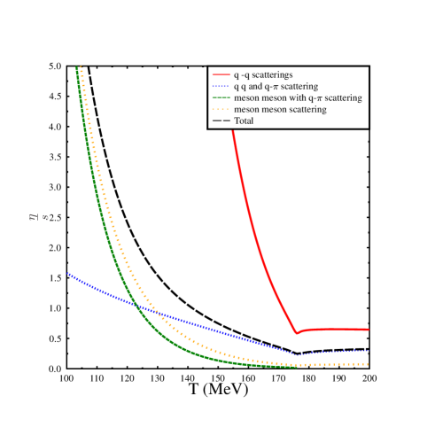
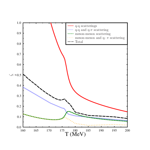
Fig. 3-a	Fig. 3-b

Figure 3: Different contributions for specific viscosity coefficients. $\eta/s$ is shown in the left while $\zeta/s$ is shown on the right. In both the figures, contributions from the quarks arising from quark quark scattering ( red solid line) and including quark meson scattering time for (blue dotted line) is shown as a function of temperature. The contribution of the mesons due to meson meson scattering (green dashed curve) and including meson quark scattering (orange short dashed curve) is also shown. The total contribution from the quarks and mesons are is shown by the black long dashed curve. All the curves correspond to $\mu=0$ case.

We now discuss about the contribution of different scatterings to the relaxation time and hence their contribution to the specific shear viscosity $\eta/s$. This is shown in Fig.3a for vanishing chemical potential. The contribution from the mesons to the shear viscosity is arising from the meson -meson scattering only is shown by the green dashed curve while the effect of including the meson quark scattering in the relaxation time estimation is shown by the orange dotted curve. Similarly the quark contribution to this ratio $\eta/s$ with a relaxation time arising from quark quark scattering is shown by the red solid line while the quark contribution to the viscosity with a relaxation time estimated including the quark pion scattering is shown by the blue dotted line. This also demonstrates the importance of the scattering of quarks and mesons to the total viscosity coefficient. The total contributions from both the quarks and mesons is shown as the black dashed curve in Fig.3a. Considering the contribution from the mesons, as may be see, including only the meson meson scattering the specific shear viscosity shows a minimum at the critical temperature with a numerical value $\eta/s\sim 0.053$which is lower than the KSS bound of $1/4\pi$. Inclusion of meson scattering with quarks however increase this value. With regards to the quark contributions (the red solid line in Fig 3a), the dominant contribution here comes from quark antiquark scattering through s-channel meson exchange. The masse of the $\sigma$-meson decreases with temperature becoming a minimum at $T_{c}$ leading to an enhancement of the cross section. Beyond $T_{c}$, the meson masses increase leading to a decrease of the cross section. This leads to a minimum of the relaxation time and hence the shear viscosity arising from quark quark scattering. Further, the effect of Polyakov loop lies in suppressing the cross section below the critical temperature as compared to e.g. Nambu JoanaLasinio modelsdeb leading to s sharp increase of the relaxation time and hence the viscosity below the $T_{c}$. However, when the quark meson scattering effects are included for one would have expected this contribution from the quark meson scattering would be suppressed due to increasing meson masses beyond $T_{c}$. However, beyond the critical temperature, there are poles in the u-channels for $q-\pi$ scattering as the $M_{\pi}$ become larger than the quark masses. This is however, regulated by the finite width of the quarks. None the less, the contribution of $q-\pi$ scatterings to the quark relaxation time remains non-negligible beyond $T_{c}$. The total contribution to the ratio $\eta/s$ is shown as black dashed curve. Clearly, the meson contributions to this ratio dominate at temperatures below $T_{c}$ while, the quark contribution dominate this ratio above $T_{c}$ as one would expect.

In a similar manner, various contributions to the specific bulk viscosity ($\zeta/s$) coefficient is shown in Fig3b. The notation regarding different contributions to $\zeta/s$ is same as in Fig.3a. As may be noted, while a peak structure is seen for the contribution arising from meson-meson scattering ( green dashed curve) at the critical temperature, such a peak is somewhat reduced when meson quark scattering is included. Similarly, for the $q-q$ scattering contribution, no such peak structure is seen and such a result is similar to what is seen in NJL models deb . On the other hand, when one includes the contribution of quark meson scatterings, a peak structure is seen for $\zeta/s$. The total effect is shown as the black dashed curve which shows a small peak structure near $T_{c}$.

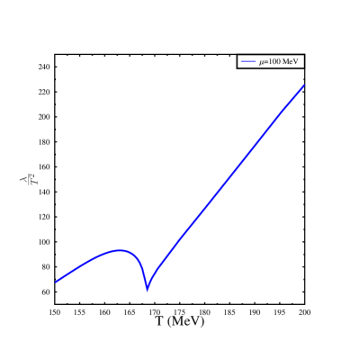
Figure 4: Thermal conductivity in units of $T^{2}$ as a function of temperature for $\mu=100$MeV.

In Fig.4, we have shown the results for thermal conductivity. We have plotted here the dimensionless quantity $\lambda/T^{2}$ as a function of temperature for $\mu=100$MeV. As is well known, thermal conductivity for relativistic particles actually diverges for $\mu=0$ and the heat conduction vanishes. However, for situations where e.g. pion number is conserved heat conductivity can be sustained by pions which themselves have zero baryon number. What we have shown in Fig.(4) is the thermal conductivity arising only from quark scattering. Similar to the behavior of relaxation time, the specific thermal conductivity has a minimum at $T_{c}$. This behavior of having a minimum at $T_{c}$ is similar to Ref.deb for NJL model. The sharp rise of $\lambda/{T}^{2}$ can be understood by performing a dimensional argument to show that at very high temperature when chiral symmetry is is restored the integral increases as $T^{3}$ while the prefactor $w/(nT)$ grows as $T^{2}$ for small chemical potentials. Apart from this kinematic consideration, as the integrand further is multiplied by $\tau(E)$ which itself is an increasing function of temperature beyond $T_{c}$, leads to the sharp rise of the ratio $\lambda/T^{2}$ beyond the critical temperature. Below, the critical temperature, however, the ratio decreases which is in contrast to NJL results of Ref.deb . The reason is two fold. Firstly the magnitude of relaxation time decrease when quark meson scattering is included as compared to quark quark scattering. This apart, in the integrand,the distribution functions are suppressed by Polyakov loops as compared to NJL model.

Summary

Transport coefficients of hot and dense matter are important inputs for the hydrodynamic evolution of the plasma that is produced following a heavy ion collision. In the present study, we have estimated coefficients taking into account the the non-perturbative effects related to chiral symmetry breaking and the confinement properties of strong interaction physics within an effective model, the Polyakov loop extended quark meson coupling model. These coefficients are estimated using relaxation time approximation for the solutions of the Boltzmann kinetic equation.

We first calculated the medium dependent masses of the mesons and quarks within a mean field approximation. The contribution of the mesons to the transport coefficients has been calculated through estimating the relaxation time for the mesons arising both from meson meson scattering and meson quark scattering. The contribution to the transport coefficients arises mostly from the meson scatterings at temperatures below the critical temperature while above the critical temperature the contributions arising from the quark scatterings become dominant. In particular, quark meson scattering contribute significantly to the relaxation time for the quarks both below and above the critical temperature. The quark pion scattering above the critical temperature gives significant contribution due to the pole structure of the corresponding scattering amplitude.

In general, the effect of Polyakov loops lies in suppressing the quark contribution below the critical temperature. This leads to, in particular, the suppression of thermal conductivity at lower temperature arising from quark scattering. The effect of Polyakov loop also is significant near and above the critical temperature. Indeed, both the quark masses as well as Polyakov loop order parameter remain significantly different from their asymptotic values near the critical temperature. It will be interesting to examine the consequences of such non-perturbative features on the transport coefficients of heavy quarks as well as on the collective modes of QGP above and near the critical temperature. Some of these works are in progress and will be reported elsewhere.

. .

References

- (1) N. Chamel and P. Hansel, Living Rev. Rel. 11, 10 (2008), arXiv:0812.3955[astro-ph]
- (2) D. G. Yakovlev, A. D. Kaminker, O. Y. Gnedin, and P. Haensel, Phys. Rept. 354, 1 (2001), arXiv:astro- ph/0012122 [astro-ph].
- (3) J. I. Kapusta,Relativistic Nuclear Collisions, Landolt-Bornstein new Series, Vol I/23, Ed. R. Stock (Springer Verlag, Berlin Heidelberg 2010).
- (4) R. Kubo,J. Phys. Soc. Jpn. 12,570,(1957).
- (5) A. Dobado,F.J.Llane-Estrada amd J. Torres Rincon, Phys. Lett. B 702, 43 (2011).
- (6) M. Bluhm, B. Kamfer and K. Redlich,Phys. Rev. C 84, 025201 (2011).
- (7) Guru Prakash Kadam, Hiranmaya Mishra,Phys. Rev. C 92, 035203 (2015);ibid,Phys. Rev. C 93, 025205 (2016); L. Thakur, P.K. Srivastava, G. Kadam, M. George,and H. Mishra,Phys. Rev. D 95, 096009 (2017).
- (8) P. Chakraborty and J.I. Kapusta Phys. Rev. C 83, 014906 (2011).
- (9) C. Sasaki and K.Redlich,Nucl. Phys. A 832, 62 (2010).
- (10) Paramita Deb, Guru Prakash Kadam, Hiranmaya Mishra, Phys. Rev. D 94, 094002 (2016).
- (11) P. Zhuang,J. Hufner, S.P. Klevansky and L. Neise,Phys. Rev. D 51, 3728 (1995).
- (12) S. Mitra and S. Sarkar, Phys. Rev. D 87, 094026 (2013), S. Mitra, S. Gangopadhyaya, S. Sarkar, Phys. Rev. D 91, 094012 (2015).
- (13) G.S. Denicol, H. Niemi, E. Molnar and D.H. Rischke,Phys. Rev. D 85, 114047 (2012).
- (14) M. Greif, F. Reining, I. Bouras , G.S. Denicol, Z. Xu and C. Greiner, Phys.Rev. E87 ,033019(2013).
- (15) G.S. Denicol, H. Niemi, I. Bouras E. Molnar , Z. Xu , D.H. Rischke, C. Greiner ,Phys. Rev. D 89, 074005 (2014).
- (16) M. Iwasaki and T. Fukutome, J. Phys. G36, 115012, 2009.
- (17) S. Nam, Mod. Phys. Lett. A 30, 1550054,2015.
- (18) D. Fernandiz-Fraile and A. Gomez Nicola, Eur. Phys. J. C 62, 37 (2009).
- (19) R. Marty, E. Bratkovskaya, W. Cassing, J. Aichelin and H . Berrehrah, Phys. Rev. C 88, 045204 (2013).
- (20) S. Ghosh, Int.J.Mod.Phys. E24 (2015) 07, 1550058
- (21) B. J. Schaefer, J. M. Pawlowski and J. Wambach, Phys. Rev. D 76, 074023 (2007).
- (22) B.W. Mintz, R.Stiele, R.O. Ramos, J.S. Bielich,Phys. Rev. D 87, 036004 (2013)
- (23) S. Carignano, M. Buballa, W.Elkamhawy,Phys. Rev. D 94, 034023 (2016)
- (24) H. Mishra, R.K. Mohapatra,Phys. Rev. D 95, 094014 (2017).
- (25) O. Scavenius, A. Mocsy, I. N. Mishustin, D. H. Rischke,Phys. Rev. C 64, 045202 (2001).
- (26) A. Bazavov etal, e-print:arXiv:1407.6387.
- (27) M. Albright and J.I. Kapusta,Phys. Rev. C 93, 014903 (2016).
- (28) Yoshimasa Hidaka, Shu Lin, Robert D. Pisarski and Daisuke Satow, JHEP10,005, (2015).
- (29) R. Lang, N. Kaiser, W. Weise, Eur. Phys. A48, 109, 2012.