Non-equilibrium electron relaxation in Graphene

Abstract

We apply the powerful method of memory function formalism to investigate non-equilibrium electron relaxation in graphene. Within the premises of Two Temperature Model (TTM), explicit expressions of the imaginary part of the Memory Function or generalized Drude scattering rate ($1/\tau$) are obtained. In the DC limit and in equilibrium case where electron temperature ($T_{e}$) is equal to phonon temperature (T), we reproduce the known results (i.e. $1/\tau\propto T^{4}$ when $T<<\Theta_{BG}$ and $1/\tau\propto T$ when $T>>\Theta_{BG}$, where $\Theta_{BG}$ is the Bloch-Grüneisen temperature). We report several new results for $1/\tau$ where $T\neq T_{e}$ relevant in pump-probe spectroscopic experiments. In the finite frequency regime we find that $1/\tau\propto\omega^{2}$ when $\omega<<\omega_{BG}$, and for $\omega>>\omega_{BG}$ it is $\omega$ independent and also electron temperature independent. These results can be verified in a typical pump-probe experimental setting for graphene.

I Introduction

Graphene is a unique two dimensional material consisting of a single atom thick layer of carbon atoms that are closely packed in honeycomb lattice structure. In recent times, the study of electronic transport of hot carriers in graphene has created an enormous research interest in both the experimental and theoretical aspects due to the potential applications in electronic devices Novoselov , Neto , Allen , Sarma , LI , NMR , Rao , Shah . In graphene, relaxation of hot (photoexcited) electrons has been investigated experimentally in Sarma , LI , Gabor , SW , KJT , Mak and theoretically in Dvgaev , Kim , Low , Iglesias , Tse , Butscher , EM , Efetov , EH , Tan , Fuhrer . In simple metals, electron relaxation dynamics is well understood and the two temperature model (TTM) is extensively used to analyze the relaxation dynamics Wong , Verburg , Majchrzak , Chen , NS , Das . While, in graphene due to Dirac physics and peculiar band structure, hot electron relaxation is different from that metal, and a detailed theoretical study is lacking.

In simple metals, hot electron relaxation happens via electron-phonon interactions. The mechanism of hot electron relaxation is as follows. A Femto-second laser pulse excites the electrons from equilibrium Fermi-Dirac (FD) distribution to a non-equilibrium distribution. This non-equilibrium electron distribution internally relaxes via electron-electron interactions to a hot FD-distribution in a time scale $\tau_{ee}$. Then through electron-phonon interactions, this “hot” FD-distribution relaxes to a state in which electron temperature becomes equal to the phonon temperature i.e., an equilibrium state. This process happens in a time scale $\tau_{e-ph}$. In simple metals the inequality $\tau_{ee}<<\tau_{e-ph}$ is true. And phonons remain in equilibrium during the whole process of relaxation (it is called the Bloch assumptionNS ). This motivates the two temperature model (TTM): one temperature for electron sub-system ($T_{e}$) and another for the phonon sub-system (T). The electron relaxation in metals is extensively studied within TTM model using the Bloch-Boltzmann kinetic equationMajchrzak , Chen , NS , Das . In the analysis an important energy scale is set by Debye temperature, and it turns out that when $T>>\Theta_{D}$, the relaxation rate from the Bloch-Boltzmann equation is given as $1/\tau\propto T$. In the opposite limit, i.e., $T<<\Theta_{D}$ it turns out that $1/\tau\propto T^{5}$.

In order to study the hot electron relaxation in graphene, several experiments like pump - probe spectroscopy and photo-emission spectroscopy has been used recently BAR , Paul , Liaros . On the theoretical side, the hot electron relaxation has been studied in graphene using the Bloch-Boltzmann equation Dvgaev , Kim , EM . But all these studies are restricted to the DC regime.

A detailed study of frequency and temperature dependent scattering rate in graphene has been lacking in the literature. In the present investigation, we solved this problem using the powerful method of memory function formalismSingh , GW , Kubo . We calculate the scattering rate in various frequency and temperature limits. Our main results are ;

In the DC case, scattering rate shows the fourth power law of both electron and phonon subsystem temperatures below the BG temperature. Above the BG temperature, scattering rate is linearly dependent on phonon temperature only. On the other hand, at higher frequency and at higher temperature, scattering rate is independent on frequency and electron temperature. It is observed that there is $\omega^{2}$-dependence in the lower frequency regime.

This paper is organized as follows. In section II, we introduce the model and memory function formalism. We then compute the memory function (generalised Drude scattering rate) using the Wölfle-Götze perturbative methodGW . Then various sub-cases are studied analytically. In section III, we present the numerical study of the general case. Finally, we summarize our results and present our conclusions.

II Theoretical Framework

To study the electron relaxation in graphene, we consider total Hamiltonian having three parts such as free electron ($H_{\text{e}}$), free phonon ($H_{\text{p}}$) and interacting part i.e electron-phonon ($H_{\text{ep}}$):

$$H = H_{\text{e}}+H_{\text{p}}+H_{\text{ep}}.$$ (1)

The different parts of Hamiltonian mentioned in the above equation are defined as

$$H_{\text{e}} = \sum_{\mathbf{k}\sigma}\epsilon_{k}c^{\dagger}_{\mathbf{k}\sigma}c_{\mathbf{k}\sigma},$$ (2)

$$H_{\text{p}} = \sum_{q}\omega_{q}\left(b^{\dagger}_{q}b_{q}+\frac{1}{2}\right),$$ (3)

$$H_{\text{ep}} = \sum_{\mathbf{k},\,\mathbf{k^{\prime}},\sigma}\left[D(\mathbf{k}-\mathbf{k^{\prime}})c^{\dagger}_{\mathbf{k}\sigma}c_{\mathbf{k^{\prime}}\sigma}b_{\mathbf{k}-\mathbf{k^{\prime}}}+\text{H.c.}\right].$$ (4)

Here, $c^{\dagger}_{\mathbf{k}\sigma}(c_{\mathbf{k}\sigma})$ and $b^{\dagger}_{q}(b_{q})$ are electron and phonon creation (annihilation) operators, $\sigma$ is a spin, $\mathbf{k}$ and $\mathbf{q}=\mathbf{k}-\mathbf{k^{\prime}}$ are electron and phonon momentum respectively. $\epsilon_{k}=\hbar v_{F}|\vec{k}|$ is the linear energy dispersion term in graphene. $D(\mathbf{k}-\mathbf{k^{\prime}})$ is the electron-phonon matrix element which is defined asEM , Mahan , Ziman

$$D(q) = -i\bigg{(}\frac{1}{2\rho_{m}\omega_{q}}\bigg{)}^{1/2}D_{0}\times q\left[1-\bigg{(}\frac{q}{2k_{F}}\bigg{)}^{2}\right]^{1/2}.$$ (5)

Here, $D_{0}$ is the deformation potential coupling constant for graphene, $\rho_{m}$ is surface mass density and $k_{F}$ is the Fermi momentum and $\omega_{q}$ is the phonon energy. Here, we set $\hbar=k_{B}=1$ throughout the calculations.

II.1 Calculation for generalized Drude scattering rate

Our aim is to calculate the generalized Drude scattering rate or imaginary part of the memory function. In a typical experimental set-up, reflectivity from a graphene sample is measured at various frequencies; and it is written as Mahan , Singh :

$$R(\omega) = \frac{(n(\omega)-1)^{2}+(k(\omega))^{2}}{(n(\omega)+1)^{2}+(k(\omega))^{2}},$$ (6)

Where,

$$n(\omega) = \frac{1}{\sqrt{2}}\sqrt{\sqrt{\epsilon_{1}^{2}(\omega)+\epsilon_{2}^{2}(\omega)}+\epsilon_{1}(\omega)},$$ (7)

$$k(\omega) = \frac{1}{\sqrt{2}}\sqrt{\sqrt{\epsilon_{1}^{2}(\omega)+\epsilon_{2}^{2}(\omega)}-\epsilon_{1}(\omega)}.$$ (8)

$\epsilon_{1}(\omega)$ and $\epsilon_{2}(\omega)$ are the real and imaginary parts of the dielectric function which are related to real and imaginary parts of the conductivity ($\sigma(\omega)$). Thus, from the reflectivity data, frequency dependent conductivity can be obtained Singh . From conductivity data, by Kramers-Kronig (KK) analysis, real and imaginary parts of the memory function are obtained as the conductivity can be written as GW :

$$\sigma(\omega) = -i\frac{1}{\omega+M(\omega)}.$$ (9)

For the calculation of generalized Drude scattering, we use the Götze-Wölfle formalism Das , Singh , LR . In this formalism, memory function is expressed as

$$M(z,T,T_{e}) = \frac{z\chi(z)}{\chi_{0}-\chi(z)}\simeq\frac{z\chi(z)}{\chi_{0}}\bigg{(}1+\frac{\chi(z)}{\chi_{0}}+....\bigg{)}$$ (10)

$$\simeq\frac{z\chi(z)}{\chi_{0}},$$

where, $\chi_{0}$ represents the static limit of correlation function (i.e. $\chi_{0}=Ne/m$) and $\chi(z)$ is the Fourier transform of the current-current correlation function:

$$\chi(z)=i\int_{0}^{\infty}e^{izt}\langle[j_{1},j_{1}]\rangle dt.$$ (11)

Here, $j_{1}=\Sigma_{k\sigma}(\vec{k}.\hat{n})c^{\dagger}_{\mathbf{k}\sigma}c_{\mathbf{k}\sigma}$ is the current density. $\hat{n}$ is the unit vector along the direction of current. Using the equation of motion (EOM) method GW , Singh it can be shown that

$$M(z,T,T_{e}) = \frac{\langle\langle[j_{1},H];[j_{1},H]\rangle\rangle_{z=0}-\langle\langle[j_{1},H];[j_{1},H]\rangle\rangle_{z}}{z\chi_{0}}.$$ (12)

Substituting equation (1) and the definition of current density operator into the above equation and on simplifying , we obtain:

$$M(z,T,T_{e}) = \frac{1}{\chi_{0}}\sum_{kk^{\prime}}\left|D(\mathbf{k}-\mathbf{k^{\prime}})\right|^{2}[(\vec{k}-\vec{k^{\prime}}).\hat{n}]^{2}$$

$$\times[{f(1-f^{\prime})(1+n))-f^{\prime}(1-f)n}]$$

$$\times\frac{1}{(\epsilon_{k}-\epsilon_{k^{\prime}}-\omega_{q})}\left[\frac{1}{(\epsilon_{k}-\epsilon_{k^{\prime}}-\omega_{q}+z)}+\frac{1}{(\epsilon_{k}-\epsilon_{k^{\prime}}-\omega_{q}-z)}\right].$$

Here, $f=f(\epsilon_{k},\beta_{e})$ and $f^{\prime}=f(\epsilon_{k^{\prime}},\beta_{e})$ are the Fermi-Dirac distribution functions at different energies such as $\epsilon_{k}$ and $\epsilon_{k^{\prime}}$ and, electron temperature $T_{e}=\frac{1}{\beta_{e}}$. $n=n({\omega_{q}},\beta)$ is the Bose-Einstein distribution function, $T=\frac{1}{\beta}$ is the phonon temperature. $z=\omega+i\delta$ and $\delta\rightarrow 0^{+}$. Here we assume a steady-state situation in which electron temperature stays constant at $T_{e}$, and phonon temperature also stays constant at T. This situation can be experimentally created by a continuous laser excitation of graphene. The memory function has real and imaginary parts: $M(z,T,T_{e})=M^{\prime}(\omega,T,T_{e})+M^{\prime\prime}(\omega,T,T_{e})$. We are interested in the scattering rate which is the imaginary part of the memory function (i.e.$M^{\prime\prime}(\omega,T,T_{e})=1/\tau(\omega,T,T_{e})$). In that case equation (LABEL:eq:MT) can be simplified to

$$\frac{1}{\tau(\omega,T,T_{e})} = \frac{\pi}{\chi_{0}}\sum_{kk^{\prime}}\left|D(\mathbf{k}-\mathbf{k^{\prime}})\right|^{2}[(\vec{k}-\vec{k^{\prime}}).\hat{n}]^{2}$$ (15)

$$\times[{f(1-f^{\prime})(1+n))-f^{\prime}(1-f)n}]$$

$$\times\frac{1}{\omega}\Bigg{[}\delta(\epsilon_{k}-\epsilon_{k^{\prime}}-\omega_{q}+\omega)-\delta(\epsilon_{k}-\epsilon_{k^{\prime}}-\omega_{q}-\omega)\Bigg{]}.$$

Converting the sums over momentum indices into integrals using the linear energy dispersion relation $\epsilon_{k}=v_{F}k$ and $\epsilon_{k}^{\prime}=v_{F}k^{\prime}$ and after further simplifying the above equation, we get,

$$\frac{1}{\tau(\omega,T,T_{e})} = \frac{1}{\tau_{0}}\int_{0}^{q_{BG}}dq\times q^{3}\sqrt{1-({q}/{2k_{f}})^{2}}$$ (16)

$$\times\Bigg{\{}(1-\frac{\omega_{q}}{\omega})\left[n(\beta,\omega_{q})-n(\beta_{e},\omega_{q}-\omega)\right]$$

$$+(\rm terms\,with\,\omega\,\rightarrow-\omega)..\Bigg{\}}.$$

Here, $1/\tau_{0}=\frac{N^{2}D_{0}^{2}}{32\pi^{3}\chi_{0}\rho_{m}k_{F}v_{s}}$ and $q_{BG}$ being the Bloch-Grüneisen momentum i.e. the maximum momentum for the phonon excitations (i.e. $v_{s}q_{BG}=2k_{F}v_{s}=\Theta_{BG}$). In graphene, a new temperature crossover known as Bloch-Grüneisen temperature ($\Theta_{BG}$) is introduced due to small Fermi surface($k_{F}$) as compared to Debye surface($k_{D}$)LR . Thus in this system when $k_{F}<<k_{D}$, below the Bloch-Grüneisen temperature, only small number of phonons with wave vector ($k_{ph}<2k_{F}$) can take part in scattering. Various limiting cases of equation (16) are studied in the next section.

II.2 Limiting cases for the generalised Drude scattering rate

Case-I: DC limit
Within this limit, curly bracket in equation (16) reduces to

$$2\lim_{\omega\to 0}\left[n(\beta,\omega_{q})-\sum_{m=0}^{\infty}\omega^{2m}\left\{\frac{\partial^{2m}}{\partial\omega_{q}^{2m}}n(\beta_{e},\omega_{q})+\omega_{q}\frac{\partial^{2m+1}}{\partial\omega_{q}^{2m+1}}n(\beta_{e},\omega_{q})\right\}\right],$$ (17)

Here we consider only m=0 i.e. the leading order case,

$$\frac{1}{\tau(\omega,T,T_{e})}=\frac{1}{\tau_{0}}\int_{0}^{q_{BG}}dq\times q^{3}\sqrt{1-\left(\frac{q}{2k_{f}}\right)^{2}}\bigg{(}n(\beta,\omega_{q})-n(\beta_{e},\omega_{q})-\omega_{q}n^{\prime}(\beta_{e},\omega_{q})\bigg{)}.$$ (18)

Using relations $\omega_{q}=v_{s}q$, $\omega_{BG}\simeq\Theta_{BG}=2v_{s}k_{F}$ and defining $\frac{\omega_{q}}{T}=x$, $\frac{\omega_{q}}{T_{e}}=y$, the above equation becomes,

$$\frac{1}{\tau(\omega,T,T_{e})} = \frac{1}{\tau_{0}}\frac{2}{v_{s}^{4}}\bigg{[}T^{4}\int_{0}^{\frac{\Theta_{BG}}{T}}dx\times\frac{x^{3}}{e^{x}-1}\sqrt{1-\left(\frac{x^{2}T^{2}}{\Theta_{BG}^{2}}\right)}+$$ (19)

$$T_{e}^{4}\int_{0}^{\frac{\Theta_{BG}}{T_{e}}}dy\times y^{3}\sqrt{1-\left(\frac{y^{2}T_{e}^{2}}{\Theta_{BG}^{2}}\right)}$$

$$\times\bigg{(}\frac{y-1}{e^{y}-1}+\frac{y}{(e^{y}-1)^{2}}\bigg{)}\bigg{]}$$

Subcase (a): $T,T_{e}<<\Theta_{BG}$, i.e., when both the phonon temperature and electron temperature are lower than the Bloch-Grüneisen temperature. Equation (19) gives

$$\frac{1}{\tau(T,T_{e})} = \frac{1}{\tau_{0}}\frac{2}{v_{s}^{4}}\bigg{[}T^{4}\times\frac{\pi^{4}}{15}+T_{e}^{4}\times\frac{\pi^{4}}{5})$$ (20)

$$= \frac{1}{\tau_{0}}\frac{2}{v_{s}^{4}}\bigg{[}A_{1}T^{4}+B_{1}T_{e}^{4}\bigg{]}.$$

Here $A_{1}=\frac{\pi^{4}}{15}$ and $B_{1}=3A_{1}$.
Subcase (b) In high temperature case, $T,T_{e}>>\Theta_{BG}$, equation (19) reduces to

$$\frac{1}{\tau(T,T_{e})} = \frac{1}{\tau_{0}}\frac{2}{v_{s}^{4}}\bigg{[}\frac{7}{30}T\Theta_{BG}^{3}+\frac{1}{6}\Theta_{BG}^{4}\bigg{]}$$ (21)

$$= \frac{1}{\tau_{0}}\frac{2}{v_{s}^{4}}\bigg{[}A_{2}T+B_{2}\bigg{]}$$

Here $A_{2}=\frac{7}{30}\Theta_{BG}^{3}$ and $B_{2}=\frac{1}{6}\Theta_{BG}^{4}$. It is notable here that the scattering rate is independent of electron temperature, and it only depends on the phonon temperature.
Subcase (c) $T>>\Theta_{BG},T_{e}<<\Theta_{BG}$. In this case scattering rate can be written as

$$\frac{1}{\tau(T,T_{e})} = \frac{1}{\tau_{0}}\frac{2}{v_{s}^{4}}\bigg{[}\frac{7}{30}T\Theta_{BG}^{3}+T_{e}^{4}\left(\frac{\pi^{4}}{5}\right)\bigg{]}$$ (22)

$$= \frac{1}{\tau_{0}}\frac{2}{v_{s}^{4}}\bigg{[}A_{3}T+B_{3}T_{e}^{4}\bigg{]}$$

Here $A_{3}=\frac{7}{30}\Theta_{BG}^{3}$ and $B_{3}=\frac{\pi^{4}}{5}$. In this case $1/\tau$ leads to the linear phonon temperature dependence in high temperature regime and shows the $T_{e}^{4}$- dependence below the BG temperature.
Subcase (d) $T<<\Theta_{BG},T_{e}>>\Theta_{BG}$. $\frac{1}{\tau(T,T_{e})}$ has $T^{4}$- dependence. Scattering rate is independent of the electron temperature. On the other hand, when $T=T_{e}$, the result of scattering rate is identical as obtained in an equilibrium electron-phonon interaction in graphene case EM , LR as expected. These results are tabulated in Table 1.
Case-II: Finite frequency regimes
Subcase (1): Consider $\omega>>\omega_{BG}$, then equation (16) becomes

$$\frac{1}{\tau(\omega,T,T_{e})} = \frac{1}{\tau_{0}}\int_{0}^{q_{BG}}dq\times q^{3}\sqrt{1-({q}/{2k_{f}})^{2}}$$ (23)

$$\times\Bigg{\{}2n(\beta,\omega_{q})-n(\beta_{e},-\omega)-n(\beta_{e},\omega)\Bigg{\}}.$$

This can be simplified by setting $\frac{\omega_{q}}{T}=x$, $\frac{\omega}{T_{e}}=\xi$, then we have

$$\frac{1}{\tau(\omega,T,T_{e})} = \frac{1}{\tau_{0}}\frac{2}{v_{s}^{4}}T^{4}\int_{0}^{\frac{\Theta_{BG}}{T}}dx\times x^{3}\sqrt{1-\left(\frac{x^{2}T^{2}}{\Theta_{BG}^{2}}\right)}$$ (24)

$$\left(\frac{2}{e^{x}-1}-\frac{1}{e^{-\xi}-1}-\frac{1}{e^{\xi}-1}\right).$$

After simplifying the above equation, it is observed that there is only the phonon contribution at higher frequency. To further simplify the above equation, we study the following subcases:

In the low temperature regime $T<<\Theta_{BG}$, equation (24) becomes

$$\frac{1}{\tau(\omega,T)} = \frac{1}{\tau_{0}}\frac{2}{v_{s}^{4}}T^{4}\bigg{[}\frac{2\pi^{4}}{15}-\frac{1}{4}\frac{\Theta_{BG}^{4}}{T^{4}}\bigg{]}$$ (25)

$$= \frac{1}{\tau_{0}}\frac{1}{v_{s}^{4}}\bigg{[}A_{5}T^{4}+B_{5}\bigg{]}$$

Here, $A_{5}=\frac{2\pi^{4}}{15}$ and $B_{5}=-\frac{\Theta_{BG}^{4}}{4}$.

In the high temperature regime $T>>\Theta_{BG}$, equation (24) takes the following form

$$\frac{1}{\tau(\omega,T)} = \frac{1}{\tau_{0}}\frac{1}{v_{s}^{4}}\bigg{[}\frac{7}{15}\Theta_{BG}^{3}T-\frac{1}{4}\frac{\Theta_{BG}^{4}}{T^{4}}\bigg{]}$$ (26)

$$= \frac{1}{\tau_{0}}\frac{1}{v_{s}^{4}}\bigg{[}A_{6}T+B_{5}\bigg{]}$$

Here $A_{6}=\frac{7}{15}\Theta_{BG}^{3}$. It is also noticeable here that in both the cases $\frac{1}{\tau(\omega,T)}$ shows the frequency independent behavior. At $T\rightarrow 0$ and higher frequency regimes, $\frac{1}{\tau(\omega)}$ shows saturation.
Subcase (2): At finite but lower frequency $\omega<<\omega_{BG}$ case, with relation $\omega_{q}=v_{s}q$ the equation (16) becomes

$$\frac{1}{\tau(\omega,T,T_{e})} = \frac{1}{\tau_{0}}\int_{0}^{\Theta_{BG}}dq\times\omega_{q}^{3}\sqrt{1-(\frac{\omega_{q}}{\Theta_{BG}})^{2}}\bigg{[}\frac{1}{e^{\frac{w_{q}}{T}}-1}-$$ (27)

$$\sum_{m=0}^{\infty}\omega^{2m}\left(\frac{\partial^{2m}}{\partial\omega_{q}^{2m}}\frac{1}{e^{\frac{w_{q}}{T_{e}}}-1}+\omega_{q}\frac{\partial^{2m+1}}{\partial\omega_{q}^{2m+1}}\frac{1}{e^{\frac{w_{q}}{T_{e}}}-1}\right)\bigg{]}$$

This is the general equation of the imaginary part of memory function when frequency is lower than the Bloch-Grüneisen frequency. The above equation can be further simplified by setting the variables $\frac{\omega_{q}}{T}=x$, $\frac{\omega_{q}}{T_{e}}=y$, and for m=1, the equation (27) reduces

$$\frac{1}{\tau(\omega,T,T_{e})} = \frac{1}{\tau_{0}}\frac{2}{v_{s}^{4}}\bigg{[}T^{4}\int_{0}^{\frac{\Theta_{BG}}{T}}dx\times x^{3}\sqrt{1-\left(\frac{x^{2}T^{2}}{\Theta_{BG}^{2}}\right)}\frac{1}{e^{x}-1}+$$ (28)

$$\omega^{2}T_{e}^{2}\int_{0}^{\frac{\Theta_{BG}}{T_{e}}}dy\times y^{3}\sqrt{1-\left(\frac{y^{2}T_{e}^{2}}{\Theta_{BG}^{2}}\right)}$$

$$\times\left(n_{y}+3n_{y}^{2}+2n_{y}^{3}-y\left(n_{y}-7n_{y}^{2}-12n_{y}^{3}-6n_{y}^{4}\right)\right)\bigg{]}$$

Here, $n_{y}=\frac{1}{e^{y}-1}$. Further we study the frequency dependent scattering rate at low and high temperature regimes of both electron and phonon sub-systems. We consider first two terms (m=0 and m=1) in the series of the equation (27). The analytic results obtained in the present subcase ($\omega<<\omega_{BG}$) are presented in Table 1. It is observed that there is $\omega^{2}$-dependence multiplied by the electron temperature in the lower frequency regime. In the general case, numerical computations of equation (16) is presented in the next section. And in the appropriate limiting cases, numerical results agree with analytical results presented in Table 1.

No	Regimes	$\frac{1}{\tau}$
1	$\omega=0;\,\,\,\,T_{e},T<<\Theta_{BG}$	$A_{1}T^{4}+B_{1}T_{e}^{4}.$
	$\omega=0;\,\,\,\,T_{e},T>>\Theta_{BG}$	$A_{2}T+B_{2}$
	$\omega=0;\,\,\,\,T>>\Theta_{BG},T_{e}<<\Theta_{BG}$	$A_{3}T+B_{3}T_{e}^{4}$.
	$\omega=0;\,\,\,\,T<<\Theta_{BG},T_{e}>>\Theta_{BG}$	$A_{4}T^{4}$+ constant.
2	$\omega>>\omega_{BG};\,\,\,\,T<<\Theta_{BG}$	$A_{5}T^{4}$.
	$\omega>>\omega_{BG};\,\,\,\,T>>\Theta_{BG}$	$A_{6}T$.
3	$\omega<<\omega_{BG};\,\,\,\,T,T_{e}>>\Theta_{BG}$	$A_{7}T+B_{7}T_{e}+C_{7}\omega^{2}T_{e}$.
	$\omega<<\omega_{BG};\,\,\,\,T,T_{e}<<\Theta_{BG}$	$A_{8}T^{4}+B_{8}T_{e}^{4}+C_{8}\omega^{2}T_{e}^{2}$.
	$\omega<<\omega_{BG};\,\,\,\,T>>\Theta_{BG},T_{e}<<\Theta_{BG}$	$A_{9}T+B_{9}T_{e}^{4}+C_{9}\omega^{2}T_{e}^{2}$.
	$\omega<<\omega_{BG};\,\,\,\,T<<\Theta_{BG},T_{e}>>\Theta_{BG}$	$A_{10}T^{4}+B_{10}T_{e}+C_{10}\omega^{2}T_{e}$.

Table 1: The results of electrical scattering rate due to the electron-phonon interactions in different limiting cases. Here, $A_{7}=\frac{7}{30}\Theta_{BG}^{3}$, $B_{7}=-\frac{7}{30}\Theta_{BG}^{3}$,$C_{7}=\frac{20}{3}\Theta_{BG}$, and $A_{8}=\frac{\pi^{4}}{15}$, $B_{8}=\frac{\pi^{4}}{5}$, $C_{8}=5\pi^{2}-\zeta(5)$ and $A_{9}=\frac{7}{30}\Theta_{BG}^{3}$, $B_{9}=\frac{\pi^{4}}{5}$, $C_{9}=C_{8}=constant$, and $A_{10}=\frac{\pi^{4}}{15}$, $B_{10}=-\frac{7}{30}\Theta_{BG}^{3}$ and $C_{10}=\frac{20}{3}\Theta_{BG}$.

III Numerical analysis

We have numerically computed the equation (16) in different frequency and temperature regimes. In Fig.1(a), we depict the phonon temperature dependence of scattering rate $1/\tau(T,T_{e})$ normalized by $1/\tau_{0}(=\frac{N^{2}D_{0}^{2}}{16\pi^{3}\chi_{0}\rho_{m}k_{F}v_{s}^{5}})$ at zero frequency and at different electron temperatures. From Fig.1(a), we observe that at high temperatures ($T_{e},T>>\Theta_{BG}$), $1/\tau(T,T_{e})\propto T$. This can also be seen in the corresponding case ($T_{e},T>>\Theta_{BG}$) in Table 1. At very low temperature ($T,T_{e}<<\Theta_{BG}$), $1/\tau\propto T^{4}\,and\,T_{e}^{4}$. Fig.1(b) shows the dependence of $1/\tau$ on $T_{e}$ in the DC limit. It is observed that $1/\tau$ is independent of $T_{e}$ when $T_{e}>>\Theta_{BG}$. Contour plots (Fig.1(c) and Fig.1(d)) depict the constant value of $1/\tau$ in $T_{e}$ and T plane. The contour for higher values of T and $T_{e}$ are for higher $1/\tau$.

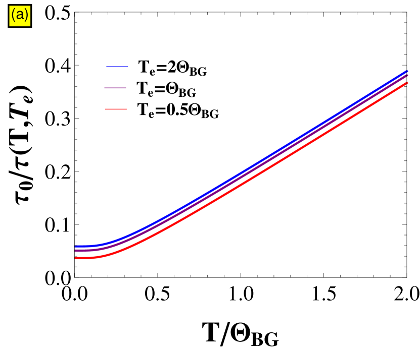
(a)

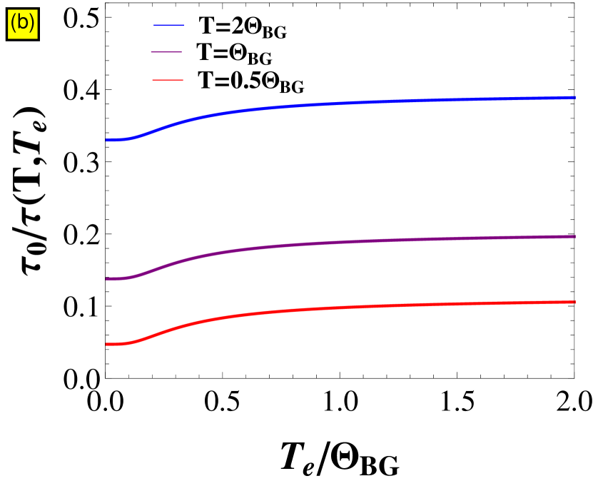
(b)

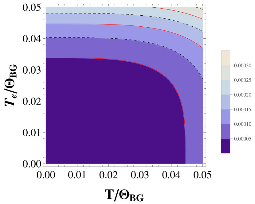
(c)

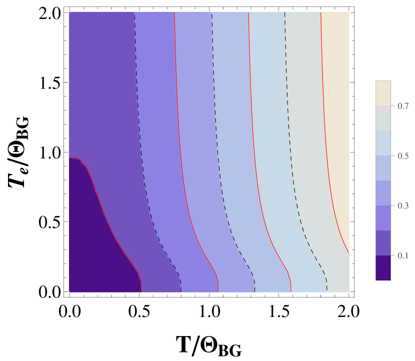
(d)

Figure 1: (a) Variation of the scattering rate with phonon temperature at zero frequency and different electron temperatures. (b) Variation of the scattering rate with electron temperature at zero frequency and different phonon temperatures. Here both the electron and phonon temperatures are scaled with the Bloch-Grüneisen temperature and $1/\tau(T,T_{e})$ is scaled with $1/\tau_{0}$. Figures (c) and (d) depict contour plots T vs $T_{e}$ for the scattering rate at zero frequency.

From the contour plots, we notice that they are not symmetric around $T=T_{e}$ line. The physical reason for this asymmetry is that the scattering rate is differently effected by phonon temperature and electron temperature (the pre-factor $A_{1}$ of $T^{4}$ term is not equal to the prefactor $B_{1}$ of $T_{e}^{4}$ terms). At very low temperature $T^{4}$ behavior is due to Pauli blocking effect. We notice that at high temperature ($T_{e},T>>\Theta_{BG}$), $1/\tau(T,T_{e})$ is proportional to $T$, not $T_{e}$. The reason for this behavior is that at high temperatures phonon modes scale as $k_{B}T(<n_{q}>=\frac{1}{e^{\beta\omega_{q}}-1}\propto k_{B}T)$, thus scattering increases with increasing temperatures linearly. For $T_{e}>>\Theta_{BG}$ the electron distribution can be approximated as Boltzmann distributions because $\Theta_{BG}\simeq T_{F}$ (the Fermi temperature). The temperature effect is exponentially reduced in this case as compared to phonons ($<n_{q}>\propto T$). Thus at high temperatures, the scattering rate is proportional to T.

In Fig.2(a), we plot the phonon temperature dependency of scattering rate $\tau_{0}/\tau(\omega,T,T_{e})$ at lower frequency and at different temperatures of electrons. It is observed that at lower phonon temperature range, the magnitude of scattering rate increases with increasing temperature as $T^{4}$ behavior. At higher T it shows T-linear behavior. In Fig.2(b), the variation of electron temperature dependence of $\tau_{0}/\tau(\omega,T,T_{e})$ at different phonon temperature scaled with BG temperature is shown. The insets of both the figures show low temperature behavior ($T,T_{e}<<\Theta_{BG}$). The low frequency behavior is similar to the DC case.

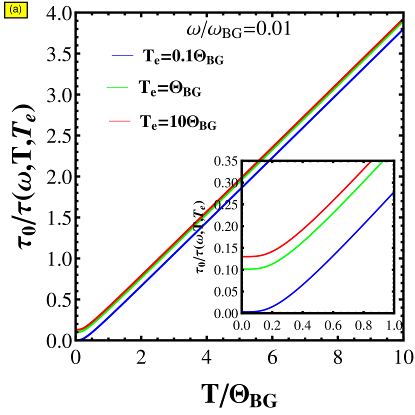
(a)

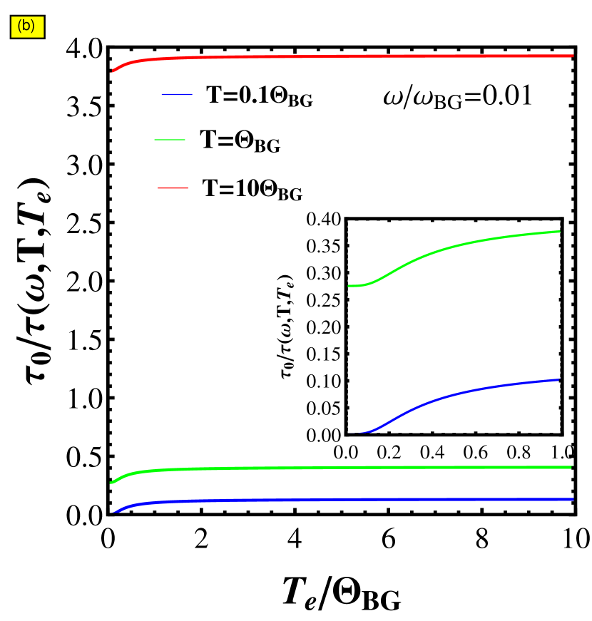
(b)

Figure 2: (a)Variation of the scattering rate with phonon temperature at finite but lower frequency and at different electron temperatures, and inset shows the lower phonon temperature range. (b)Variation of the scattering rate with electron temperature at finite frequency and at different phonon temperatures, and inset shows the lower electron temperature range.

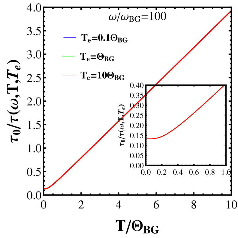
(a)

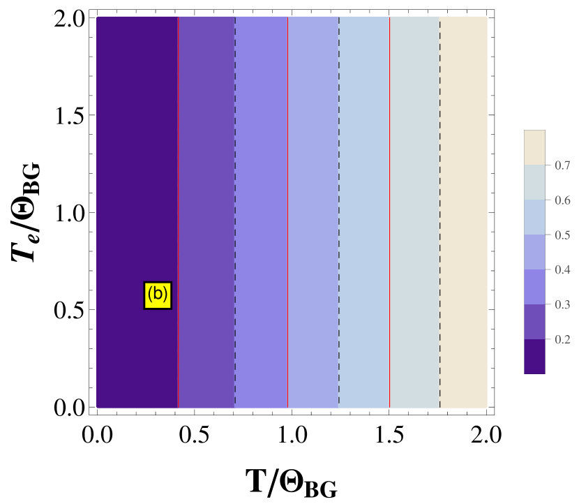
(b)

Figure 3: (a)Variation of the scattering rate with phonon temperature at higher frequency ($\omega/\omega_{BG}=100$) and at different electron temperatures, and inset shows the same plot with lower phonon temperature range over $\Theta_{BG}$. The inset also shows finite scattering rate even at zero phonon temperature which is nothing but the non-equilibrium generalization of the Holstein mechanism Das , Singh , LR . (b) The contour plot depicts the behavior of scattering rate at higher frequency ($\omega/\omega_{BG}=100$).

In order to study the higher frequency regime, we plot the variation of the scattering rate with phonon temperature at higher frequency ($\omega/\omega_{BG}=100$) and at different electron temperatures in Fig.3(a). It is observed that at higher frequency, scattering rate is independent of the electron temperature (compare with the corresponding entry given in Table 1). Plot shows the T-linear behavior above BG temperature and $T^{4}$ behavior below lower BG temperature. These results agree with the result of Efetov , EH . At higher frequency, the scattering rate is controlled by phonon temperature. The independence of $1/\tau$ from $T_{e}$ is also shown in the contour plot (Fig.3(b)).

We further analyzed the scattering rate at zero temperature in which both electron subsystem and phonon subsystem are at zero temperature. In this regime $1/\tau$ scales as $\omega^{4}$ as depicted in Fig.4.

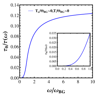
Figure 4: (a)Variation of the scattering rate with frequency at zero electron and phonon temperatures, and inset shows the same plot at lower frequency over Bloch-Grüneisen frequency.

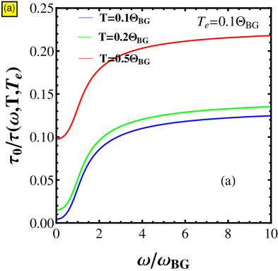
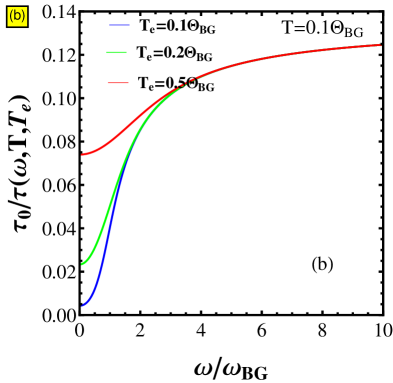
Figure 5: Variation of the scattering rate with frequency at different electron and phonon temperatures.

To order to study the scattering rate with frequency, we plot the frequency dependence behavior of the scattering rate $1/\tau(\omega,T,T_{e})$ at different temperatures of electron and phonon subsystems in Fig.5. Fig.5(a) depicts the variation of scattering rate with frequency at different phonon temperatures and at fixed electron temperature. At higher frequency, $1/\tau$ saturates and at lower frequency it shows $\omega^{2}$ behavior.

In Fig.5(b), we plot the variation of scattering rate with frequency at different electron temperatures and fixed phonon temperature. From Fig.5(b), it is clear that on increasing the electron temperature, scattering rate increases in lower frequency regime but scattering rate goes into saturation trend in the high frequency regimes, and become independent of electron temperature. This can also be obtained from Table 1 (in the $\omega>>\omega_{BG}$ case).

IV Conclusion and discussion

We presented a theoretical study of non-equilibrium relaxation of electrons due to their coupling with phonons in graphene by using the memory function approach. In our results at zero frequency limit, it is observed that if both the electron and phonon temperature are not same, DC scattering rate has a fourth power law behavior of both the electron and phonon temperaures i.e. ($A_{1}T^{4}+B_{1}T_{e}^{4}$) below the BG temperature. While at higher temperature, $1/\tau$ shows the T-linear dependency only (it does not depend on $T_{e}$). Further, it is important to notice here that DC scattering rate and AC scattering rate shows the similar T-linear behavior at higher temperature.

No	Regimes	Graphene $\bigg{(}\dfrac{1}{\tau}\bigg{)}$	Metals $\bigg{(}\dfrac{1}{\tau}\bigg{)}$Das
		2D	3D
		Bloch Grünisen	Debye
		Temperature $(\Theta_{BG})$	Temperature $(\Theta_{D})$
1	$\omega=0;\,\,\,\,T_{e},T<<\Theta_{BG},\Theta_{D}$	$A_{1}T^{4}+B_{1}T_{e}^{4}.$	$a_{1}T^{5}+b_{1}T_{e}^{5}.$
	$\omega=0;\,\,\,\,T_{e},T>>\Theta_{BG},\Theta_{D}$	$A_{2}T$.	$a_{2}+b_{2}T$
	$\omega=0;\,\,\,\,T>>\Theta_{BG},T_{e}<<\Theta_{BG}$	$A_{3}T+B_{3}T_{e}^{4}$.	-
	$\omega=0;\,\,\,\,T<<\Theta_{BG},T_{e}>>\Theta_{BG}$	$A_{4}T^{4}$.	-
2	$\omega>>\omega_{BG},\omega_{D};\,\,\,\,T>>\Theta_{BG},\Theta_{D}$	$A_{5}T$.	$a_{3}+b_{3}T$.
	$\omega>>\omega_{BG},\omega_{D};\,\,\,\,T<<\Theta_{BG},\Theta_{D}$	$A_{6}T^{4}$.	$a_{4}+b_{4}T^{5}$
3	$\omega<<\omega_{BG},\omega_{D};\,\,\,\,T,T_{e}>>\Theta_{BG},\Theta_{D}$	$A_{7}T+B_{7}T_{e}+C_{7}\omega^{2}T_{e}$.	$a_{5}T+b_{5}\omega^{2}T_{e}$
	$\omega<<\omega_{BG},\omega_{D};\,\,\,\,T,T_{e}<<\Theta_{BG},\Theta_{D}$	$A_{8}T^{4}+B_{8}T_{e}^{4}+C_{8}\omega^{2}T_{e}^{2}$.	$a_{6}T^{5}+b_{6}T_{e}^{5}+c_{6}T_{e}^{5}\omega^{2}$
	$\omega<<\omega_{BG};\,\,\,\,T>>\Theta_{BG},T_{e}<<\Theta_{BG}$	$A_{9}T+B_{9}T_{e}^{4}+C_{9}\omega^{2}T_{e}^{2}$.	-
	$\omega<<\omega_{BG};\,\,\,\,T<<\Theta_{BG},T_{e}>>\Theta_{BG}$	$A_{10}T^{4}+B_{10}T_{e}+C_{10}\omega^{2}T_{e}$.	-

Table 2: Comparison of non-equilibrium electron relaxation in metals and in graphene

In Table 2, we compare the results of scattering rates for the simple metals and the present case of graphene. We observed that $T^{5}$-law of $1/\tau$ in the case of metals (in regimes $\omega=0,\,T<<\Theta_{D}$) changes to $T^{4}$-law in the corresponding case in graphene. However, in the case of high temperatures and high frequencies, temperature dependence of $1/\tau$ in both metals and in graphene remains the same.

At higher frequency, the scattering rate is controlled by phonon temperature in both the cases (of metals and graphene). In the low frequency case ($\omega<<\omega_{D}$) and in lower temperature regimes ($T,T_{e}<<\Theta_{D}$) $1/\tau$ in metals has three terms ($a_{6}T^{5}+b_{6}T_{e}^{5}+c_{6}T_{e}^{5}\omega^{2}$) whereas in the corresponding case of graphene this dependence changes to ($A_{8}T^{4}+B_{8}T_{e}^{4}+C_{8}\omega^{2}T_{e}^{2}$). These results can be verified that in a typical pump-probe experiments Shah , Verburg , Liaros .

References

• [1] K. S. Novoselov, A. K. Geim, S. V. Morozov, D. Jiang, M. I. Katsnelson, I. V. Grigorieva, S. V. Dubonos and A. A. Firsov (2005) Two-dimensional gas of massless Dirac fermions in graphene Nature 438 197
• [2] A. H. Castro Neto, F. Guinea, N. M. R. Peres, K. S. Novoselov and A. K. Geim (2009) The electronic properties of graphene Rev. Mod. Phys. 81 109
• [3] M. J. Allen, V. C. Tung and R. B. Kaner (2010) Honeycomb carbon: a review of graphene Chem. Rev. 110 132
• [4] S. D. Sarma, S. Adam, E. H. Hwang and E. Rossi (2011) Electronic transport in two-dimensional graphene Rev.Mod. Phys. 83 407
• [5] Z. Q. Li, E. A. Henriksen, Z. Jiang, Z. Hao, M. C. Martin, P. Kim, H. L. Stormer and D. N. Basov (2008) Dirac charge dynamics in graphene by infrared spectroscopy Nat. Phys. Lett. 4 532
• [6] N. M. R. Peres, T Stauber and A. H. C. Neto (2008) The infrared conductivity of graphene on top of silicon oxide Euro. Phys. Lett. 84 38002
• [7] C. N. R. Rao, A. K. Sood, K. S. Subrahmanyam, and A. Govindaraj (2009) , Graphene: The New Two-Dimensional Nanomaterial Angew. Chem. Int. Ed. 48 7752
• [8] J. Shah, Hot Carrier in Semiconductor Nanostructures (Academic,London, 1992).
• [9] N. M. Gabor (2011) Hot carrier–assisted intrinsic photoresponse in graphene Science 334 648-652
• [10] S. Winnerl and M. Orlita (2011) Carrier Relaxation in Epitaxial Graphene Photoexcited Near the Dirac Point, Phys. Rev. Lett. 107, 237401
• [11] K. J. Tielrooij, L. Piatkowski, M. Massicotte, A. Woessner, Q. Ma,Y. Lee, K.S. Myhro, C. N. Lau, P. Jarillo-Herrero, N. F. van Hulst and F. H. L. Koppens (2015) Generation of photovoltage in graphene on a femtosecond timescale through efficient carrier heating Nature Nanotechnology 10 437
• [12] K. F. Mak , M. Y. Sfeir, Y. Wu, C H Lui, J. A. Misewich and T. F. Heinz (2008) Measurement of the Optical Conductivity of Graphene Phys. Rev. Lett. 101 196405
• [13] V. K. Dugaev and M. I. Katsnelson (2013) Edge scattering of electrons in graphene: Boltzmann equation approach to the transport in graphene nanoribbons and nanodisks, Phys. Rev. B 88 235432
• [14] R. Kim, V. Perebeinos and P. Avouris (2011) Relaxation of optically excited carriers in graphene, Phys.Rev. B 84 075449
• [15] T. Low, V. Perebeinos, R. Kim, M. Freitag and P. Avouris (2012) Cooling of photoexcited carriers in graphene by internal and substrate phonon, Phys. Rev. B 86 045413
• [16] J. M. Iglesias, M. J. Martín, E. Pascual, and R. Rengel (2016) Hot carrier and hot phonon coupling during ultrafast relaxation of photoexcited electrons in graphene, Appl. Phys. Lett. 108 043105
• [17] W.-K. Tse and S. D. Sarma (2009) Energy relaxation of hot electrons in graphene Phys. Rev. B 79 235406
• [18] S. Butscher, F. Milde (2007) Hot electron relaxation and phonon dynamics in graphene Appl. Phys. Lett. 91 203103
• [19] E. Muñoz (2012) Phonon-limited transport coefficients in extrinsic graphene J. Phys.: Condens. Matter 24 195302 .
• [20] D. K. Efetov and P. Kim (2010) Controlling electron-phonon interactions in Graphene at ultrahigh carrier densities Phys. Rev. Lett. 105 256805
• [21] E. H. Hwang and S. D. Sarma (2008) Acoustic phonon scattering limited carrier mobility in two-dimensional extrinsic graphene Phys. Rev. B 77, 115449
• [22] Y.-W Tan, Y. Zhang , H. L. Stormer and P Kim (2007) Temperature dependent electron transport in graphene Eur. Phys. J. Special Topics148 15
• [23] M. S. Fuhrer (2010) Textbook physics from a cutting-edge material Phys. 3 106
• [24] B. T. Wong and M. P.Mengüç (2008) Two-Temperature Model Coupled with e-Beam Transport. In: Thermal Transport for Applications in Micro/Nanomachining. Microtechnology and MEMS. Springer, Berlin, Heidelberg
• [25] P. C. Verburg, G. R. B. E. Römer A. J. Huis in ’t Veld (2014) Two-temperature model for pulsed-laser-induced subsurface modifications in Si Appl. Phys. A 114 1135
• [26] E. Majchrzak, J. Dziatkiewicz (2012 ) Application of the Two-Temperature Model for a numerical study of multiple laser pulses interactions with thin metal films Sci. Res. Inst. Math. Comput. Sci. 11 63-70
• [27] J. K. Chen, D. Y. Tzou, J. E. Beraun (2006) A semiclassical two-temperature model for ultrafast laser heating Int.J. of Heat and Mass Transfer 49 307
• [28] N. Singh (2010) Two-Temperature Model of non equilibrium electron relaxation: a review Int. J. Mod. Phys. B 24, 1141
• [29] N. Das and N. Singh (2016) Hot electron relaxation in metals within the Götze-Wölfle memory function formalism Int. J. Mod. Phys. B 30 1650071
• [30] B. A. Ruzicka, S. Wang, J. Liu, K.-P. Loh, J. Z. Wu and H. Zhao (2012) Spatially resolved pump-probe study of single-layer graphene produced by chemical vapor deposition Optical Material Express 2 708
• [31] P. A. George, J. Strait, J. Dawlaty, S. Shivaraman (2008) Ultrafast Optical-Pump Terahertz-Probe Spectroscopy of the Carrier Relaxation and Recombination Dynamics in Epitaxial Graphene Nano Lett. 12 4248
• [32] N. Liaros, S. Couris, E. Koudoumas and P. A. Loukakos (2016) Ultrafast Processes in Graphene Oxide during Femtosecond Laser Excitation J. Phys. Chem. C, 120 (7), 4104
• [33] W. Götze and P. Wölfle (1972) Homogeneous dynamical conductivity of simple metals Phys. Rev. B 6 1226
• [34] R. Kubo (1957) Statistical-mechanical theory of irreversible processes. I. General theory and simple applications to magnetic and conduction problems J. Phys. Soc. Japan 12 570
• [35] N. Singh (2016) Electronic Transport Theories: From Weakly to Strongly Correlated Materials (Taylor and Francis Group, CRC Press)
• [36] G. D. Mahan (2000) Many-Particle Physics (Physics of Solids and Liquids), Kluwer Academic/Plenum Publishers
• [37] J. M. Ziman (2001) Electrons and Phonons: The Theory of Transport Phenomena in Solids (Oxford Classic Texts in the Physical Sciences)
• [38] L. Rani and N. Singh (2017) Dynamical electrical conductivity of graphene, J. Phys.: Condens. Matter 29 255602 .