Transverse mode coupling instability of the bunch
with oscillating wake field and space charge

Abstract

Transverse mode coupling instability of a single bunch caused by oscillating wake field is considered in the paper. The instability threshold is found at different frequencies of the wake with space charge tune shift taken into account. The wake phase advance in the bunch length from 0 up to $4\pi$ is investigated. It is shown that the space charge can push the instability threshold up or down dependent on the phase advance. Transition region is investigated thoroughly, and simple asymptotic formulas for the threshold are represented.

I INTRODUCTION

The transverse mode coupling instability (TMCI) of a bunch with both wake field (WF) and space charge (SC) was first considered in paper Bl1 . It has been shown there that, at a moderate ratio of the SC tune shift to the synchrotron tune $(\Delta Q/Q_{s})$, the SC pushes up threshold of the instability caused by a negative wake. Hereafter the result has been confirmed in papers Bu1 -Bl2 .

However, more confusing picture appears at the larger value of this ratio like a hundred or over. It has been suggested in Ref. Bu1 that the threshold growth ceases behind this border coming to 0 at $\,\Delta Q/Q_{s}\rightarrow\infty$. By contrast, it was asserted in Ref. Ba1 that negative wake cannot excite the TMCI in this limiting case.

An explanation of the collision has been proposed in Ref. Ba2 where it has been noted that approximate methods of solution were applied in all mentioned articles. Typically, an expansion of the bunch coherent displacement in terms of some series of basic functions was used there, with subsequent truncation of the series. It turns out that, with this approach, the TMCI threshold can strongly and not monotonously depend from the actual number of used basic functions.

The problem has been clarified in recent publication Ba3 where the method of solution has been developed which does not use the expansion technique at all, and therefore is applicable at arbitrary SC tune shift. In particular, it has been shown that the TMCI threshold of negative wakes is asymptotically proportional to $\,\Delta Q/Q_{s}$ in contrast with the case of positive wake whose threshold is $\,\propto Q_{s}/\Delta Q$. The statement has been extended in the paper on any monotonous WF, e.g. on the resistive wall impedance.

In the presented paper, this method is applied for investigation of oscillating (resonant) wake fields. It is shown that the SC tune shift can suppress or intensify the instability, dependent on the wake phase advance from the bunch head to its tail. It is shown as well that, at some conditions, the dependence of the TMCI rate on the wake amplitude is a non-monotonic function.

Some of these problems were considered earlier using other models and techniques of the calculations Ba2 , Bu2 . All the results are in rather good consent to be convinced of applicability of the used methods. Their detailed comparison is carried out at the end of Sec. V.

II PHYSICAL MODEL

Following Ba3 , we represent the bunch transverse coherent displacement in the rest frame as the part of the function

$$\bar{X}(z,t)=\bar{Y}(z)\exp\big{[}-iQ_{\beta}(z/R+\Omega_{0}t)-i\Omega_{0}\nu t\big{]}$$ (1)

where $\,z$ is the longitudinal coordinate, $\,t\,$ is time, $\,R$ is the machine radius, $\,\Omega_{0}$ is the revolution frequency, $\,Q_{\beta}$ and $\,\nu$ are the central betatron tune and the addition to it due to the wake field. The machine chromaticity in not included in the expression as a factor of a small importance for the TMCI threshold Ba2 .

In framework of the model, it is convenient to use another longitudinal coordinate $\,\vartheta\propto z$ which is adjusted to the bunch located on the interval $\,0\leq\vartheta\leq\pi$. Then the rearranged function $\,\bar{Y}$ satisfies the equation

$$Q_{s0}^{2}\bar{Y}^{\prime\prime}(\vartheta)+\nu\hat{\nu}\bar{Y}(\vartheta)=\frac{2\hat{\nu}}{\pi}\int_{\vartheta}^{\pi}q(\vartheta^{\prime}-\vartheta)\bar{Y}(\vartheta^{\prime})\,d\vartheta^{\prime}$$ (2)

with the boundary conditions

$$\bar{Y}^{\prime}(0)=\bar{Y}^{\prime}(\pi)=0$$ (3)

where $\,Q_{s0}$ is the synchrotron tune, and $\,\hat{\nu}=\nu+\Delta Q$ with $\,\Delta Q$ as the space charge tune shift Ba3 . The function $\,q(\vartheta)$ is proportional to the usual transverse wake function at corresponding distance $\,W_{1}(z_{\vartheta})$:

$$q(\vartheta)=\frac{r_{0}RN_{b}W_{1}}{8\pi\beta^{2}\gamma Q_{\beta}}$$ (4)

where $\,r_{0}=e^{2}/mc^{2}$ is the particle electromagnetic radius, $\,N_{b}$ is the bunch population, $\,\beta$ and $\,\gamma$ are the normalized velocity and energy of the particles.

The oscillating wake of the form

$$q(\vartheta)=q_{0}\exp(-\alpha\theta)\cos\kappa\vartheta$$ (5)

will be considered in this paper. Then Eq. (2) obtains the form

$$\bar{Y}^{\prime\prime}(\vartheta)+{\cal P}\bar{Y}(\vartheta)=$$

$$\frac{2{\cal Q}}{\pi}\exp(\alpha\theta)\int_{\vartheta}^{\pi}\exp(-\alpha\theta^{\prime})\cos\kappa(\vartheta^{\prime}-\vartheta)\bar{Y}(\theta^{\prime})\,d\vartheta^{\prime}$$ (6)

with the notations

$${\cal P}=\frac{\nu\hat{\nu}}{Q_{s0}^{2}},\qquad{\cal Q}=\frac{q_{0}\hat{\nu}}{Q_{s0}^{2}}$$ (7)

It is easy to see that the integral-differential Eq. (6) is reducible to the net differential equation of $4^{th}$ order:

$$\bar{Y}^{IV}-\alpha\bar{Y}^{\prime\prime\prime}+({\cal P}+\kappa^{2})\bar{Y}^{\prime\prime}+$$

$$\left(\frac{2{\cal Q}}{\pi}-\alpha{\cal P}\right)\bar{Y}^{\prime}+\kappa^{2}{\cal P}\bar{Y}=0$$ (8)

with boundary conditions given by Eq. (3) and more

$$\bar{Y}^{\prime\prime}(\pi)=-{\cal P}\bar{Y}(\pi),\qquad\bar{Y}^{\prime\prime\prime}(\pi)=-\frac{2{\cal Q}}{\pi}\,\bar{Y}(\pi).$$ (9)

Similar in appearance equations of third order were considered in Ref. Ba3 . Like them, it is possible to solve Eq. (8) step-by-step starting from the point $\,\vartheta=\pi$ with initial conditions

$$\bar{Y}(\pi)=1,\qquad\bar{Y}^{\prime}(\pi)=0,$$ (10a)

$$\bar{Y}^{\prime\prime}(\pi)=-{\cal P},\qquad\bar{Y}^{\prime\prime\prime}(\pi)=\!-\frac{{\cal Q}}{\pi}$$ (10b)

and going down to the point $\,\vartheta=0$. Some trial value of $\,\cal{P}$ has to be used each time with chosen parameters $\,\kappa,\;\alpha$ and $\,{\cal Q}$; however, only those of them resulting in the relation $\,Y^{\prime}(0)=0$ should be taken as the valid solutions satisfying all the required conditions. With any $\,\cal Q$, there is an infinite discrete sequence of the eigennumbers $\;{\cal P}_{n}$ satisfying these conditions.

III EIGENNUMBERS OF THE EQUATION

It is the general requirement for applicability of the single bunch approximation that the damping coefficient is large enough to neglect the bunch-to-bunch or the turn-by-turn interaction. However, it does not exclude that the damping is negligible within the bunch: $\,\exp(-\pi\alpha)\simeq 1$. Therefore the case $\,\alpha=0$ is considered for the beginning.

Several eigennumbers of Eq. (8) are represented in Figs. 1-3 where different frequencies of the wake are considered (the used value of $\,\kappa$ is designated right in the graph). Six lowest real eigennumbers $\,{\cal P}_{n}$ are plotted against $\,{\cal Q}$ in each the case. As one would expect, $\,{\cal P}_{n}=n^{2}$ at $\,{\cal Q}=0$ independently on $\,\kappa$. The index $\,n$ will be used further to mark the lines.

The overall behavior of the plots considerably depends on the frequency. The upper graph $(\kappa=0.5)$ is similar to the case of rectangular wake $\,\kappa=0$, both qualitative and quantitative Ba3 . The next case $\,\kappa=1$ has a different appearance because its lowest line $\,n=0$ outspreads far to the right where it connects with the upper line $\,n=5$. Figure 3 with $\,\kappa=1.5$ differs ever stronger because it contains the lines $\,n=0$ and $\,n=1$ starting together in the point $\,{\cal Q}\simeq-1$ and separately going to the right.

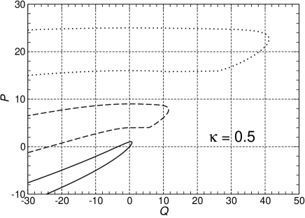
Figure 1: Several lowest real eigennumbers of Eq. (6) and Eq. (8) at $\,\alpha=0,\;\kappa=0.5$. The picture insubstantially differs from the case of rectangular wake $\,\kappa=0$ Ba3 . In particular, numbers of the coalescence lines are: $\,n=$ (0,1); (2,3); (4,5); etc. All the lines diverge at $\,{\cal Q}\rightarrow-\infty.$

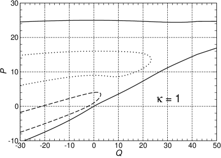
Figure 2: The same as in Fig. 1 at $\,\kappa=1$. The main difference is other combinations of the coalesced modes. In particular, the modes $\,n=0$ and $\,n=5$ join smoothly at $\,{\cal Q}\simeq 70$.

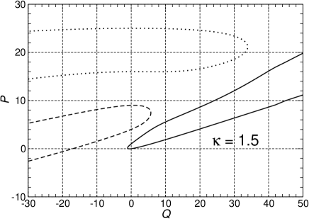
Figure 3: The same as Fig. 1 at $\,\kappa=1.5$. The main difference is that real parts of the modes $\,n=0$ and $\,n=1$ are coalecsed at $\,{\cal Q}<-1$, and diverge at $\,{\cal Q}\rightarrow\infty$.

IV THE BUNCH EIGENTUNES

Obtained functions $\,{\cal P}_{n}(\cal{Q)}\,$ have to be imaged into the plane $\,(q_{0},\hat{\nu})\,$ with help of the transformations

$$\hat{\nu}_{\pm n}=\frac{\Delta Q}{2}\pm\sqrt{\frac{\Delta Q^{2}}{4}+{\cal P}_{n}Q_{0}^{2}},\qquad q_{0}=\frac{Q_{0}^{2}{\cal Q}}{\hat{\nu}_{\pm n}}$$ (11)

which follow from Eq. (7). Any point of the family is the real eigentune of the bunch with given SC tune shift. They form several lines representing tunes of different head-tail modes which depend on the wake frequency.

As it has been shown above, $\,{\cal P}_{n}=n^{2}$ at $\,{\cal Q}=0$. Corresponding solutions are Bu1 :

$$\hat{\nu}_{\pm n}=\frac{\Delta Q}{2}\pm\sqrt{\frac{\Delta Q^{2}}{4}+n^{2}Q_{0}^{2}},\qquad{\rm at}\qquad q_{0}=0$$ (12)

At $\,\Delta Q=0$, it results in $\,\hat{\nu}_{m}=mQ_{s0}$ where $\,m=\pm n$. Such oscillations are known as multipoles. Any eigenmode of the bunch is a combination of several multipoles. Nevertheless, the multipole numbers $\,m$ can be used for the classification of the lines in the plots. For example, a line index $\,\,m=-2$ means that the line passes through the point $\,\hat{\nu}=-2\,\Omega_{s0}$ at $\,q_{0}=0$ and $\,\Delta Q=0$. An important role in this consideration play coalescing curves. We will use the symbol $\,m=(m_{1},m_{2})$ to mark the coalescence of the lines of kinds $\,m_{1}$ and $\,m_{2}$.

Using Figs. 1-3 and Eq. (11), one can get the bunch tunes at selected wake frequency and different $\,\Delta Q$. Some results are plotted in Figs.4-6 where the solid or the dashed lines are used repeating appearance of the origin blocks of Figs. 1-3. Different colors are used in the resulting figures for different SC tune shifts: $\,\Delta Q=0$ (blue), or $\,\Delta Q/Q_{s0}=1.5$ (green), or $\,\Delta Q/Q_{s0}=3$ (red). The extreme points of the lines characterized by the relation $\,dq_{0}=0$ highlight beginning of the instability regions.

The case $\,\kappa=0.5$ is represented in Fig. 4. It bears the great resemblance to the case of $\,\kappa=0$ which has been considered in Ref. Ba3 with help of the square wake model. In particular, the blue lines form the chart which is well known as the TMCI tunes without space charge $\,\Delta Q=0$ (see e.g. Ng1 ). At $\,\kappa=0.5$, the instability appears because of coalescence of the modes $\,m=0$ and $\,m=\pm 1$ having the threshold $|q_{0}|/Q_{s0}$ = 0.81 (0.57 at $\,\kappa=0$ or with the square wake model).

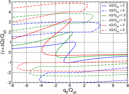
Figure 4: The bunch eigentunes with different $\,\Delta Q$ at $\,\kappa=0.5$

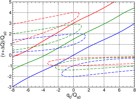
Figure 5: The bunch eigentunes with different $\,\Delta Q$ at $\,\kappa=1$. The same legends as in Fig. 4 are used.

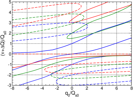
Figure 6: The bunch eigentunes with different $\,\Delta Q$ at $\,\kappa=1.5$ The same legends as in Fig. 4 are used.

All the lines move to the left-up at increasing $\,\Delta Q$. It means formally that the TMCI threshold increases in modulus tending to $-\infty$ at $\,q_{0}<0$, and decreases tending to 0 at $\,q_{0}>0$. The coinciding results have been obtained with the square wake model Ba3 . However, only the case $\,q_{0}<0$ has a physical sense for the oscillating wake given by Eq. (5). It means that the SC tune shift stabilizes the TMCI, at least at $\,\kappa\leq 0.5$. It is necessary to take into account that the mode $\,m=(-2,-3)$ depends less on $\,\Delta Q$ and moves slower to the left than the mode $\,m=(0,-1)$. Therefore it is the most unstable at $\,\Delta Q/Q_{s0}<\sim 5-6$. It has been stated in Ref. Ba3 at $\,\kappa=0$, and remains in force at the moderate value of $\,\kappa$.

Similar picture takes place at $\,\kappa=1$ (Fig. 5). The main difference is that the instability appears because of a coalescence of the modes $\,m=-1$ and $\,m=-2$ which effect has the threshold $\,q_{0}/Q_{s0}=-1.56$ at $\,\Delta Q=0$ (the dashed blue lines). The mode $\,m=0$ could participate only by the coalescence with the mode $\,m=-5$ which is possible at much higher amplitude of the wake beyond the graph.

Very different picture has a place at $\,\kappa=1.5$ as it follows from Fig. 6. At $\,\Delta Q=0$, the instability arises by a coalescence of the modes $\,m=-2$ and $\,m=-3$ having the threshold $\,q_{0}/Q_{s0}=-2.13$ (dashed blue lines). However, the lower modes $\,m=0$ and $\,m=1$ come in to play at $\,\Delta Q\neq 0$ resulting in the instability with the threshold $\,q_{0}/Q_{s0}=-0.66$ at $\,\Delta Q/Q_{s0}=1.5$ and $\,q_{0}/Q_{s0}=-0.34$ at $\,\Delta Q/Q_{s0}=3$. The appearance of positive multipoles as well as the lowering of the TMCI threshold at increasing $\,\Delta Q$ is the characteristic of a positive wake Ba3 . It is an expected effect in the case because the wake is mostly positive in the bunch at $\,q_{0}<0$ and phase advance $\,1.5\pi$.

Evolution of the spectral lines $\,m=0$ and $\,m=1$ at $\,\kappa=1.5$ and increasing $\,\Delta Q$ is represented in more details in Fig. 7. The blue lines, showing their initial position at $\,\Delta Q=0$, move toward each other to meet at $\,\Delta Q/Q_{s0}\simeq 0.3$ and to split up in other direction immediately after that. The magenta lines show their position and shape at $\,\Delta Q/Q_{s0}=0.35$. It is seen that very narrow region of instability $\,-3.5<q_{0}/Q_{s0}<-3$ arises in this case. However, it expands very rapidly at increasing $\,\Delta Q$ obtaining the location $\,-7.0<q_{0}/Q_{s0}<-1.3$ at $\,\Delta Q/Q_{s0}=0.7$ (brown lines), and $\,-11.4<q_{0}/Q_{s0}<-0.7$ at $\,\Delta Q/Q_{s0}=1.5$ (green lines) Nevertheless, the bunch does take stable in the left ot this area because threshold of the mode $\,m=(-1,-2)$ is essentially lower as it follows from Fig. 6.

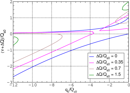
Figure 7: The lowest bunch mode $\,m=(0,1)$ as a function of the wake amplitude at $\,\kappa=1.5$ and different $\,\Delta Q/Q_{s0}$. At $\,\Delta Q/Q_{s0}>0.35$, the mode becomes unstable at sufficiently large $\,q_{0}$ but obtains the stability again at the further increase of the wake. However, the bunch can remain unstable because of excitation of the mode $\,m=(-2,-3)$.

V THE INSTABILITY THRESHOLD

The developed method allows to find the TMCI threshold with any set of parameters. Some results are represented in this section.

Dependence of the threshold on the wake frequency is shown in Fig. 8 at $\,\Delta Q/Q_{s0}=0$, 1.5, and 3. One can see the oscillations of the threshold and the slow growth of its average value with frequency at $\,\kappa>1.5$, which effects have to be expected. However, the most important conclusion is that the SC stabilizes the TMCI at $\,\Delta Q/Q_{s0}<1$ and destabilizes it at $\,\Delta Q/Q_{s0}>1.5$. The transition takes place rather rapidly at $\,\Delta Q\simeq 1.25$.

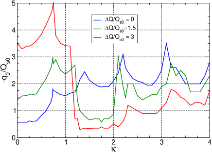
Figure 8: The TMCI threshold against the wake frequency at relatively low space charge tune shift. The shift stabilizes the bunch at $\,\kappa<1$ and destabilizes it at $\,\kappa>1.5$.

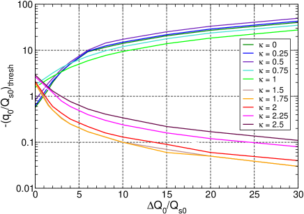
Figure 9: The TMCI threshold against the SC tune shift at different wake frequencies. The parts with frequencies $\,\kappa<1$ and $\kappa>1.5$ are clearly separated.

.

Dependence of the threshold on the SC tune shift is shown in Fig. 9 over a wider range of the parameters. The most remarkable effect is that the lines representing different wake frequencies are distinctly broken down into two groups: with upper threshold at $\,\Delta Q/Q_{s0}<1$ and with lower one at $\,\Delta Q/Q_{s0}>1.5$. They have different asymptotic behavior: $\,q_{0}\sim\Delta Q$ in the upper group and $\,q_{0}\sim Q_{s0}^{2}/\Delta Q$ in the lower one. Such a behavior can be obtained with help of Eq. (11) at the assumption

$$|{\cal P}|\ll(\Delta Q/2Q)^{2}.$$ (13)

With sign ’–’ before the root, it gives

$$\hat{\nu}\simeq-\frac{{\cal P}Q_{s0}^{2}}{\Delta Q},\qquad q_{0}\simeq-\frac{\cal Q}{\cal P}\Delta Q$$ (14)

According these equations, the value of $\,q_{0}$ varies when the point $({\cal Q},{\cal P})$ moves along one of the curves like shown in Fig. 4 or Fig. 5. The TMCI threshold obtained by the last Eq. (14) appears in the point where the condition $\,dq_{0}=0$ is fulfilled that is $\,d{\cal P}/{\cal P}=d{\cal Q}/{\cal Q}$. It is the point of tangency of the curve with the straight line ${\cal P}=k_{tg}{\cal Q}$. Therefore the asymptotic expression for the threshold is:

$$q_{0}=k_{th}\Delta Q$$

where the constant depends on the wake frequency $\,\kappa$ as it is represented in Table I

Another possibility follows from Eq. (11) and Eq. (13) with sign ’+’ before the root:

$$\hat{\nu}\simeq\Delta Q,\qquad q_{0}\simeq\frac{{Q_{s0}^{2}\cal Q}}{\Delta Q}$$

According these equations the value of $\,q_{0}$ varies when the point $({\cal Q},{\cal P})$ moves along one of the curves like shown in Fig. 6. The relation $\,dq_{0}=0$, that is $\,d{\cal Q}=0$, should be applied additionally to find the instability threshold. It follows from Fig. 6 that the corresponding value of the $\,{\cal Q}_{ex}\simeq-1.1$ at $\kappa=1.5$. Other values are represented in Table II. The results are in a conflict with the output of Ref. Bu1 where it is predicated that the space charge has almost no affects on the TMCI threshold at $\,\kappa=2$.

Table 1: Dependence of the asymptotic coefficients on the wake frequency: $q_{0}=k_{tg}(\kappa)\Delta Q$

$~{}~{}\kappa$	0	0.25	0.5	0.75	1
$~{}~{}k_{tg}~{}~{}$	-1.34	-1.43	-1.65	-1.17	-0.92

Table 2: Dependence of the asymptotic coefficients on the wake frequency: $q_{0}=Q_{s0}^{2}{\cal Q}_{ex}(\kappa)/\Delta Q$

$~{}~{}\kappa$	1.5	1.75	2	2.25	2.5
$~{}~{}{\cal Q}_{ex}~{}~{}$	-1.1	-1.1	-1.3	-2.4	-3.4

The data submitted in Fig. 9 at $\,\kappa\leq 1$ are in a good agreement with results of the paper Ba2 where synchrotron oscillations in a parabolic potential well have been studied using the standard expansion technique. TMCI in the parabolic well has been considered also in recent paper Bu2 on the base of the asymptotic equations at $\,\Delta Q\gg Q_{s0}$. The coincidence of the plots like shown in Fig. 8 confirms that the TMCI threshold is not very sensitive to used models of the bunch and of the potential well. The thresholds presented in Fig. 9 at $\,\kappa>1.5$ are in a satisfactory quantitative compliance with the ”non-vanishing TMCI” of Ref. Bu2 where the square well model has been used also but other algorithm of the calculations has been applied.

VI TRANSITIONAL WAKE FREQUENCY.

The broad blank area between the top and bottom parts of Fig. 9 is assigned for the wake of the frequency $\,1<\kappa<1.5$. However, the transition is not a smooth process in the case. Actually, at constant SC tune shift and increasing wake, the instability can arise, disappear, appear again in other form, etc. This statement is illustrated below on the example of the wake with $\,\kappa=1.25$.

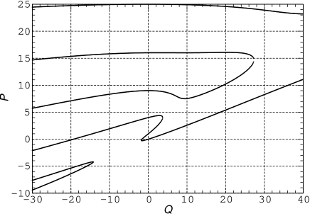
Figure 10: Several lowest real eigennumbers of Eq. (6) and Eq. (8) at $\,\alpha=0,\;\kappa=1.25$. In comparison with Figs. 2 and 3, there is an additional curl of the lower line

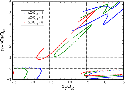
Figure 11: The bunch eigentunes at the wake parameters $\,\alpha=0,\,\kappa=1.25$. The eigentunes at $\,\Delta Q/Q_{s0}=4$ are shown by dotted blue lines the lower of them representing the mode $\,m=(-2,-3)$. There are the islands of stability at $\,\Delta Q/Q_{s0}=5$ and 6 (green and red ovals).

Several lowest eigennumbers of Eq. (8) are shown on Fig. 10. The distinction from Figs. 1-3 consists in the appearance of the additional curl with the branches starting from the point $\,{\cal Q}\simeq-14,\,{\cal P}\simeq-4$ and steering to the left and down. It leads to appearance of the specific areas on the plane $(q_{0},\hat{\nu})$ which are shown on Fig. 11. Like Fig. 7, instability of the mode $\,m=(0,-1)$ appears not at once but at sufficiently large SC tune shift. For example, with $\,\Delta Q/Q_{s0}=1$, the instability arises at $\,q_{0}/Q_{s0}\simeq-3$. However, it disappears already at $\,q_{0}/Q_{s0}\simeq-3.1$ that is, in practice, the instability is behind the scenes at such tune shift. Other examples are given in Fig. 11 where the larger tune shifts are considered. It is seen that the instability band extends very quickly at increasing $\,\Delta Q$ reaching approximately the area $-17<q_{0}/Q_{s0}<-0.5$ at $\,\Delta Q/Q_{s0}=4$ This case is shown by the blue lines in the top-right corner and in the bottom-left one of Fig. 11. It should be noted that the mode $\,m=(-2,-3)$ has the threshold $\,q_{0}/Q_{s0}=-4.7$ at $\,\Delta Q/Q_{s0}=4$ which tune is shown by the blue dotted line in the bottom-right corner of Fig. 11. Therefore, with such SC tune sift, the broad picture is:

The bunch is stable at $\,|q_{0}/Q_{s0}|<0.5$;

The mode $\,m=(0,-1)$ becomes unstable at

$0.5<|q_{0}/Q_{s0}|<4.7$;

Both modes $\,m=(0,-1)$ and $\,m=(-2,-3)$

are unstable at $\,4.7<|q_{0}/Q_{s0}|<17$;

Only the mode $\,m=(-2,-3)$ is unstable at

$\,|q_{0}/Q_{s0}|>17$.

At larger SC tune shifts, the picture becomes even more complicated because of an appearance of the additional islands of stability of the mode $\,m=(0,-1)$. They are shown in Fig. 11 by green and red ovals related to the cases $\,\Delta Q/Q_{s0}=5$ or 6, correspondingly. As a result, following picture is played e.g. at $\,\Delta Q/Q_{s0}=6$ (red lines):

The bunch is stable at $|q_{0}/Q_{s0}|<0.3$;

The mode $\,m=(0,-1)$ becomes unstable at

$\,0.3<|q_{0}/Q_{s0}|<2.8$;

The instability disappears at $2.8<|q_{0}/Q_{s0}|<6.4$;

The mode $\,m=(-2,-3)$ becomes unstable at

$6.4<|q_{0}/Q_{s0}|<18.2$;

Both modes $\,m=(0,-1)$ and $\,m=(-2,-3)$

are unstable at $\,18.2<|q_{0}/Q_{s0}|<24.8$;

Only the mode $\,m=(-2,-3)$ remains unstable at

$\,|q_{0}/Q_{s0}|>24.8$;

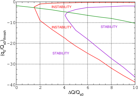
Figure 12: Thresholds of different bunch modes at $\,\kappa=1.25$. Red and violet: $\,m=(0,-1)$, green: $\,m=(-2,-3)$.

The process is illustrated also by Fig. 12. The mode $\,m=(0,-1)$ may be unstable in the regions between the red lines, or between the red and the violet lines but not between the violet lines. The legends in the picture concern namely this mode. Another mode $\,m=(-2,-3)$ is unstable everywhere below the green line. The asymptotic of this threshold is $\,q_{0}=-0.9\Delta Q$ which expression is quite coordinated with Table II.

Thus, with the oscillating wake, the TMCI threshold can be a nonmonotonic function of both the SC tune shift and the WF amlitude. The result is similar to that found in Ref. Bl1 in framework of the expansion technique.

VII Conclusions

The TMCI threshold of the oscillating wake without space charge increases at increase of the wake frequency. The space charge effect depends on the wake phase advance on the bunch length $\,\phi$.

At $\,\phi<\pi$, the threshold is about proportional to the space charge tune shift $\,\Delta Q$.

At $\,\phi>1.5\pi$, the threshold is about $\,\propto Q_{s}^{2}/\Delta Q$ with $\,Q_{s}$ as the synchronron tune.

At $\,\phi\simeq 1.25\pi$, the TMCI threshold can be a non-monotonic function of both the space charge tune shift and the wake amplitude. The variability occurs because different multipole numbers are responsible for the instability at different conditions.

The phase advance more of $4\pi$ is not considered in the paper.

VIII Acknowledgment

Fermi National Accelerator Laboratory is operated by Fermi Research Alliance, LLC under Contract No. DEAC02-07CH11395 with the United States Department of Energy.

References

- (1) M. Blaskiewicz, Fast head-tail instability with space charge, Phys. Rev. ST Accel. Beams 1, 044201 (1998).
- (2) A. Burov, Head-tail modes for strong space charge, Phys. Rev. ST Accel. Beams 12, 044202 and 12, 109901 (2009).
- (3) V. Balbekov, Transverse instability of a bunched beam with space charge and wakefield, Phys. Rev. ST Accel. Beams 14, 094401 (2011).
- (4) M. Blaskiewicz, Comparing new models of transverse instability with simulations, in Proceedings of the 3rd International Particle Accelerator Conference. New Orleans, LA, 2012 (IEEE, Piscataway, NJ, 2012)
- (5) V. Balbekov, Transverse mode coupling instability with space charge and different wakefields, Phys. Rev. Accel. Beams 20, 034401 (2017).
- (6) V. Balbekov, Threshold of transverse mode coupling instability with arbitrary space charge, Phys. Rev. Accel. Beams 20, 114401 (2017).
- (7) T. Zolkin, A. Burov, B. Pandey, TMCI and Space Charge II, http://arxiv.org/pdf/1711.11110/pdf (2017).
- (8) B. Ng, Report No. Fermilab-FN-07-13 (2002).