DESY 18-005

Higgs Inflation at the LC
W. G. Hollik

Deutsches Elektronen-Synchrotron (DESY),

Notkestraße 85, D-22607 Hamburg, Germany.

Most cosmological models of inflation are far away from providing a smoking gun at low energies. A model of Higgs inflation in the Next-to-Minimal Supersymmetric Standard Model, however, changes the NMSSM phenomenology drastically and may be well distinguished from the pure NMSSM or MSSM at a future Linear Collider. We point out certain differences of the inflationary model to the ordinary NMSSM and discuss the Higgs and neutralino/chargino sector in particular to identify the smoking gun of inflation at electroweak energies.

Talk presented at the International Workshop on Future Linear Colliders (LCWS2017), Strasbourg, France, 23-27 October 2017. C17-10-23.2

1 Introduction

Cosmological models that can be tested in the laboratory are typically very rare. A smoking gun at low energies of a model acting at a very large scale like the Planck scale requires a precision machine like a Linear Collider. Precise electroweak observations may then distinguish between an ordinary extension of the Standard Model (SM) or an extension which simultaneously grasps cosmological problems. Early universe inflation is to be seen as a cosmological fact which has to be addressed. If it is addressed in a way that interrelates the Planck-scale physics with Fermi-scale physics, such a model will most probably modify the Higgs sector of the SM. On an economic basis, employing the SM Higgs field as the inflaton field of cosmology, such a model can be called minimal. While Higgs inflation in the SM tends to become “unnatural” towards the high scales, see Ref. [1], a more viable candidate is the scale-free Supersymmetric Standard Model. The scale-free model requires compared to the Minimal Supersymmetric Standard Model (MSSM) an additional singlet superfield and thus is known as the Next-to-Minimal Supersymmetric Standard Model (NMSSM).

The Higgs sector of the NMSSM is characterised by the $\mathbb{Z}_{3}$-invariant superpotential

$$\mathcal{W}_{\text{Higgs}}=\lambda\;\hat{S}\,\hat{H}_{u}\cdot\hat{H}_{d}+\frac{\kappa}{3}\;{\hat{S}}^{3},$$ (1)

where $\hat{H}_{u}$ and $\hat{H}_{d}$ are the $\mathrm{SU}(2)_{L}$ doublet Higgs superfields and $\hat{S}$ the singlet superfield. The scalar components of the doublet fields decompose as

$$H_{u}=\begin{pmatrix}H_{u}^{+}\\ H_{u}^{0}\end{pmatrix},\qquad H_{d}=\begin{pmatrix}H_{d}^{0}\\ H_{d}^{-}\end{pmatrix},$$ (2)

such that $H_{u}\cdot H_{d}=H_{u}^{+}H_{d}^{-}-H_{u}^{0}H_{d}^{0}$. This superpotential has an accidental $\mathbb{Z}_{3}$-invariance under the transformation

$$\hat{\Phi}\to e^{i\frac{2\pi}{3}k}\hat{\Phi},\quad k\in\mathbb{Z},\quad\text{for }\hat{\Phi}=\hat{H}_{u},\hat{H}_{d},\hat{S},$$

such that only trilinear terms are allowed. Especially the $\mu$-term of the MSSM, $\mu\;H_{u}\cdot H_{d}$, is forbidden if the $\mathbb{Z}_{3}$ symmetry is imposed. After electroweak symmetry breaking, however, the singlet scalar acquires a vacuum expectation value (vev) and dynamically induces a $\mu$-term via the $\lambda$ coupling, which plays the role of an effective higgsino mass term:

$$\mu_{\text{eff}}=\lambda\langle S\rangle.$$ (3)

Non-minimal coupling in Canonical Superconformal Supergravity

The implementation of Higgs inflation in superconformal theories follows the non-minimal coupling of the Higgs field content to supergravity, as suggested by Ref. [1], and comes with a single dimensionless and holomorphic coupling $X(\hat{\Phi})$:

$$\mathcal{L}=-6\int\operatorname{d}^{2}\theta\mathcal{E}\left[R+X(\hat{\Phi})R-\frac{1}{4}\left(\bar{\mathcal{D}}^{2}-8R\right){\hat{\Phi}}^{\dagger}\hat{\Phi}+\mathcal{W}(\hat{\Phi})\right]+\text{h.\,c.\ }+\ldots,$$ (4)

where $\mathcal{E}$ is the vierbein multiplet, $R$ the curvature multiplet and $\bar{\mathcal{D}}$ a covariant derivative. The chiral superfields $\hat{\Phi}$ shall be any of the fields $H_{u}$, $H_{d}$ or $S$. A realization of such a non-minimal coupling involving the doublet Higgs fields only can be found to be

$$X=\chi\;\hat{H}_{u}\cdot\hat{H}_{d},$$ (5)

with a numerical factor $\chi$. Note that this term breaks the $\mathbb{Z}_{3}$ symmetry of the NMSSM and the superconformal symmetry.

The addition of the superconformal symmetry breaking term changes the frame function in Jordan frame supergravity and affects the Kähler potential in such a way that the NMSSM superpotential gets modified [2, 3]. In Planck units ($M_{P}=1$), the frame function $\Omega=\hat{\Phi}_{i}^{*}\hat{\Phi}_{i}-3$ gets extended by the $\chi$-term to

$$\Omega_{\chi}=\Omega-\frac{3}{2}\left(X(\hat{\Phi})+\text{h.\,c.\ }\right),$$ (6)

and similarly the Kähler potential

$$\mathcal{K}=-3\log(-\Omega/3)\to\mathcal{K}_{\chi}=-3\log(-\Omega_{\chi}/3).$$ (7)

In the canonical superconformal supergravity (CSS) model, the frame function is explicitly given by [4, 3]

$$\Omega_{\text{CSS}}=-3+|\hat{S}|^{2}+|\hat{H}_{u}|^{2}+|\hat{H}_{d}|^{2}+\frac{3}{2}\chi\left(\hat{H}_{u}\cdot\hat{H}_{d}+\text{h.\,c.\ }\right).$$ (8)

In order to have successful inflation in the NMSSM, however, a stabilisator term $\zeta(\hat{S}\hat{\bar{S}})^{2}$ has to be added [4, 3], which disappears from the low-energy phenomenology (Planck-suppressed).

The $\chi$-term breaks a continuous $\mathcal{R}$ symmetry and its discrete $\mathbb{Z}_{3}$ subgroup at dimension six $\sim\chi\tfrac{\lambda^{2}h^{6}}{M_{P}^{2}}$. Much below the Planck scale, the additional term induces a correction in the superpotential

$$\mathcal{W}_{\text{eff}}\to\mathcal{W}e^{\frac{3}{2}\chi H_{u}\cdot H_{d}/M_{P}^{2}}\approx\mathcal{W}+\frac{\langle\mathcal{W}_{\text{hid}}\rangle}{M_{P}^{2}}\frac{3}{2}\chi H_{u}\cdot H_{d}\equiv\mathcal{W}+\frac{3}{2}\chi m_{3/2}H_{u}\cdot H_{d},$$ (9)

where the vev of the hidden sector superpotential can be related to the gravitino mass scale

$$m_{3/2}\approx\frac{\langle\mathcal{W}_{\text{hid}}\rangle}{M_{P}^{2}}.$$ (10)

Effectively, the superpotential of the NMSSM gets modified by an additional $\mu$-like term,

$$\mathcal{W}_{\text{iNMSSM}}=\lambda\;SH_{u}\cdot H_{d}+\frac{\kappa}{3}\;S^{3}+\mu\;H_{u}\cdot H_{d},$$ (11)

with $\mu=\frac{3}{2}\chi m_{3/2}$. Thus, the effective higgsino mass term of the NMSSM Eq. (3) gets shifted by the contribution from the non-minimal coupling to supergravity leading to inflation as

$$\mu_{\text{eff}}^{\prime}=\lambda\;\langle S\rangle+\frac{3}{2}\chi m_{3/2}=\mu_{\text{eff}}+\mu.$$ (12)

The low-energy smoking gun of Higgs inflation in the superconformal setup appears to be the NMSSM extended with an MSSM-like $\mu$-term and can be quite well distinguished from either the pure MSSM or NMSSM as will be discussed in the following. We refer to this model setup as the inflationary NMSSM, or short iNMSSM.

2 A short introduction to the iNMSSM

We consider the NMSSM extended with the additional $\mu$-term as described above only. Its presence can be motivated from a non-minimal coupling to supergravity and a proceeding transformation in the Kähler potential in such a way that only the term $\mu\;H_{u}\cdot H_{d}$ is present in the superpotential with $\mu=\frac{3}{2}\chi m_{3/2}$. Cosmological observations require the size of this non-minimal coupling to be

$$\chi\simeq 10^{5}\lambda.$$ (13)

The size of the $\mu$-term is then mainly given by the gravitino mass $m_{3/2}$ and the $\lambda$ coupling, which we will assume to be $\mathcal{O}(0.1)$ in order to have sizeable NMSSM effects. Generically, we also assume $\mu\sim\mathcal{O}(1\,\mathrm{TeV})$, which in combination requires rather light gravitinos of $m_{3/2}\sim 10\,\mathrm{MeV}$. This might cause the cosmological gravitino problem, see Ref. [5]. Overabundance of gravitino dark matter, however, can be constrained by constraining the reheating temperature after inflation [6]. We assume that the details of the inflationary model can accommodate this problem as outlined in [3].

Soft SUSY breaking in the iNMSSM and the Higgs potential

The additional $\mathds{Z}_{3}$-breaking $\mu$-term may generate an additional soft Supersymmetry (SUSY) breaking bilinear parameter in a similar manner as the Higgs $B_{\mu}$-term exists in the MSSM. All further $\mathds{Z}_{3}$-breaking soft SUSY breaking terms that are in general allowed, see [7] and [8], are assumed to be suppressed [9] and cannot be generated to sizeable amount by radiative corrections. Therefore, the soft SUSY breaking potential can be summarised as the usual trilinear terms of the NMSSM $\sim A_{\lambda},A_{\kappa}$ plus the bilinear term from the non-minimal coupling to supergravity:

$$V_{\text{soft}}=\lambda A_{\lambda}\,SH_{u}\cdot H_{d}+\frac{1}{3}\kappa A_{\kappa}\,S^{3}+\frac{3}{2}B_{\mu}\chi m_{3/2}\left(H_{u}\cdot H_{d}+\text{h.\,c.\ }\right).$$ (14)

The scalar potential for the two doublet and one singlet Higgs fields is defined according to the rules of SUSY and consists of the $F$- and $D$-terms as well as the contribution from SUSY breaking. In comparison to the $\mathds{Z}_{3}$-symmetric NMSSM, we have the additional $\mu$-term appearing as mass term for the doublet fields and the bilinear soft breaking term $\sim H_{u}\cdot H_{d}$. The full Higgs potential is thus given by

$$V_{\text{Higgs}}= \left[m_{H_{d}}^{2}+(\mu+\lambda S)^{2}\right]|H_{d}|^{2}+\left[m_{H_{u}}^{2}+(\mu+\lambda S)^{2}\right]|H_{u}|^{2}+m_{S}^{2}\,|S|^{2}$$ (15)

$$+\frac{2}{3}\kappa A_{\kappa}\,S^{3}+\left[\kappa\,S^{2}+\lambda\,H_{u}\cdot H_{d}\right]^{2}+2\left(B_{\mu}\mu+\lambda A_{\lambda}\,S\right)H_{u}\cdot H_{d}$$

$$+\frac{g_{1}^{2}+g_{2}^{2}}{8}\left(|H_{d}|^{2}-|H_{d}|^{2}\right)^{2}+\frac{g_{2}^{2}}{2}|H_{d}^{\dagger}H_{u}|^{2},$$

where we assume all parameters to be real.

The potential of Eq. (15) can easily provide the observed phenomenology of electroweak symmetry breaking meaning Higgs vevs of the neutral doublet Higgs field components, $\langle H^{0}_{u}\rangle=v_{u}$ and $\langle H^{0}_{d}\rangle=v_{d}$, with $v_{u}^{2}+v_{d}^{2}=v^{2}=(174\,\mathrm{GeV})^{2}$ and $\tan\beta=v_{u}/v_{d}$ a free parameter; additionally, the singlet vev generates the effective $\mu$-term of the NMSSM, $\mu_{\text{eff}}=\lambda\langle S\rangle=\lambda v_{s}$. In order to do so, the soft SUSY breaking masses $m_{H_{d}}^{2}$, $m_{H_{u}}^{2}$ and $m_{S}^{2}$ are adjusted in such a way, that the minimisation conditions

$$\frac{\partial V_{\text{Higgs}}}{\partial H^{0}_{d}}\bigg{|}_{\text{vev}}=\;2m_{H_{d}}^{2}v_{d}+\ldots,\leavevmode\nobreak\ \frac{\partial V_{\text{Higgs}}}{\partial H^{0}_{u}}\bigg{|}_{\text{vev}}=\;2m_{H_{u}}^{2}v_{u}+\ldots,\leavevmode\nobreak\ \frac{\partial V_{\text{Higgs}}}{\partial S}\bigg{|}_{\text{vev}}=\;2m_{H_{d}}^{2}v_{s}+\ldots$$ (16)

are fulfiled. Solving for the mass parameters is trivial and we obtain

$$m_{H_{d}}^{2} =-(\mu+\mu_{\text{eff}})^{2}-v^{2}\lambda^{2}\sin^{2}\beta-\frac{1}{2}M_{Z}^{2}\cos(2\beta)+a_{1}\tan\beta,$$ (17a)

$$m_{H_{u}}^{2} =-(\mu+\mu_{\text{eff}})^{2}-v^{2}\lambda^{2}\cos^{2}\beta+\frac{1}{2}M_{Z}^{2}\cos(2\beta)+a_{1}\cot\beta,$$ (17b)

$$m_{S}^{2} =a_{4}-a_{5}-a_{7}-v^{2}\lambda^{2}-2\mu_{\text{eff}}^{2}\left(\frac{\kappa}{\lambda}\right)^{2},$$ (17c)

where $M_{Z}^{2}=\tfrac{g_{1}^{2}+g_{2}^{2}}{2}v^{2}$ and the abbreviations $a_{i}$ are defined in Appendix A.

The electroweak breaking conditions have to be taken with great care, since the potential possesses multiple minima and even if one particular minimum is selected to be the electroweak (desired) vacuum by the above definition, there might be other minima deeper than the desired vacuum and thus the true vacuum, i. e. the global minimum, is not the desired one anymore. At tree-level, the minimisation can only be done numerically; at the loop-level, the situation even gets worse and one has to guess suitable starting values for the numerical routines, which have the potential to miss several of the minima. We take those constraints at the tree-level seriously and therefore exclude parameter points leading to a non-standard true vacuum of the theory. Typically, this global minimum appears at larger vevs for the fields and thus gets more easily selected by the cosmological history of the universe after inflation [10]. Since we start with vevs shortly below the Planck scale after inflation ends, the universe while cooling down may get stuck in the higher scale vacuum. If it is a local minimum, one should consider the tunneling to the desired one. Typically, however, the larger vev vacuum appears to be deeper than the desired vacuum.

Besides the fact that there are multiple vacua implying alternative vevs in the Higgs potential, the Higgs mass matrices (defined in Appendix A) show tachyonic states at the tree-level depending on the input parameters. Tachyonic states have negative masses squared and simply invalidate the electroweak expansion point because the potential at that point appears to be a local maximum (the “minimisation” conditions are rather conditions for stationary points and may also result in maxima or saddle points) and thus pointing towards the deeper minimum in the tachyonic direction. Actually, radiative corrections may lift up the potential in some cases leading to rather light instead of tachyonic states. We take these constraints nevertheless seriously and exclude tachyonic parameter configurations irrespective whether radiative corrections lift the masses up or not.

The tachyonic constraints already confine clear portions of parameter space that remain valid. In addition, vacuum stability considerations exclude additional parts at the borderline.

3 Electroweak phenomenology of the iNMSSM

The phenomenology of the iNMSSM at the electroweak scale deviates significantly from the usual NMSSM. On the one hand, the number of states remain the same which may look like the same phenomenology. On the other hand, the dependence on certain parameters appears to be very different and the additional $\mu$-term changes the interpretation of the higgsino mass parameter as well as the functional dependence of the Higgs masses on it.

First of all, the tachyonic selection rule excludes large as well as very small ($\lesssim\sqrt{2}v$) values of $\mu_{\text{eff}}$. Moreover, both values $\mu$ and $\mu_{\text{eff}}$ appear to be correlated. This can be seen from Figure 1. The tachyonic boundaries can be easily understood from a look at the mass matrices, see Appendix A, where the small $\mu_{\text{eff}}$ value sets $A_{\lambda}$ to be large, which sits on the off-diagonal elements and thus is responsible for a large mixing which potentially drives one state negative. Similarly, if the combination $\mu+\mu_{\text{eff}}$ appears to be large; therefore same signs of $\mu$ and $\mu_{\text{eff}}$ are excluded in most cases. The trilinear soft SUSY breaking parameter $A_{\kappa}$ mainly influences the pseudoscalar singlet-like state. If this one appears to be tachyonic for small $A_{\kappa}$, larger values of this parameter have the ability to lift this mass up and open up parameter space that is excluded with a vanishing $A_{\kappa}$. This can be clearly seen in the comparison of the allowed and excluded parameter space in the $\mu$-$\mu_{\text{eff}}$-plane shown in Figure 1.

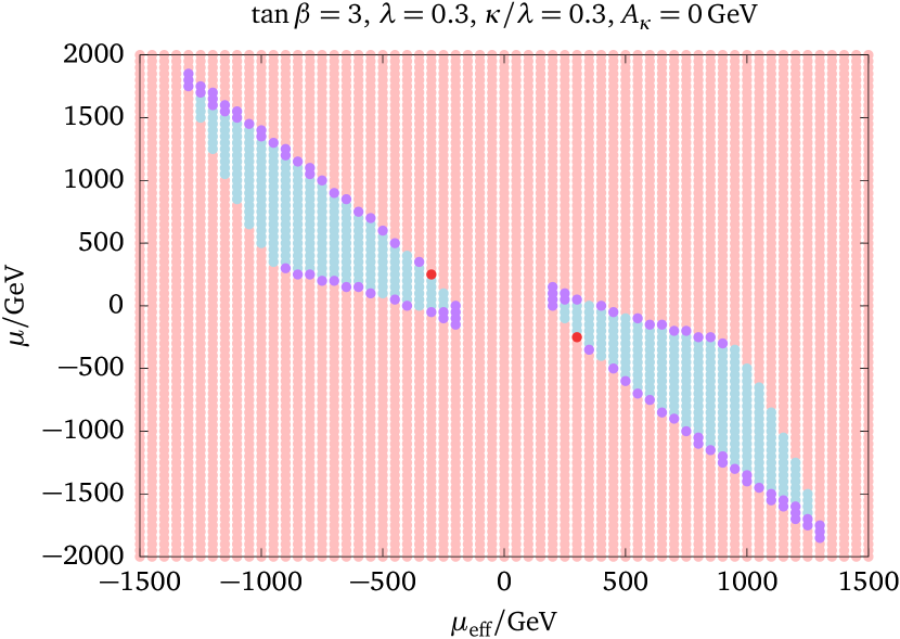
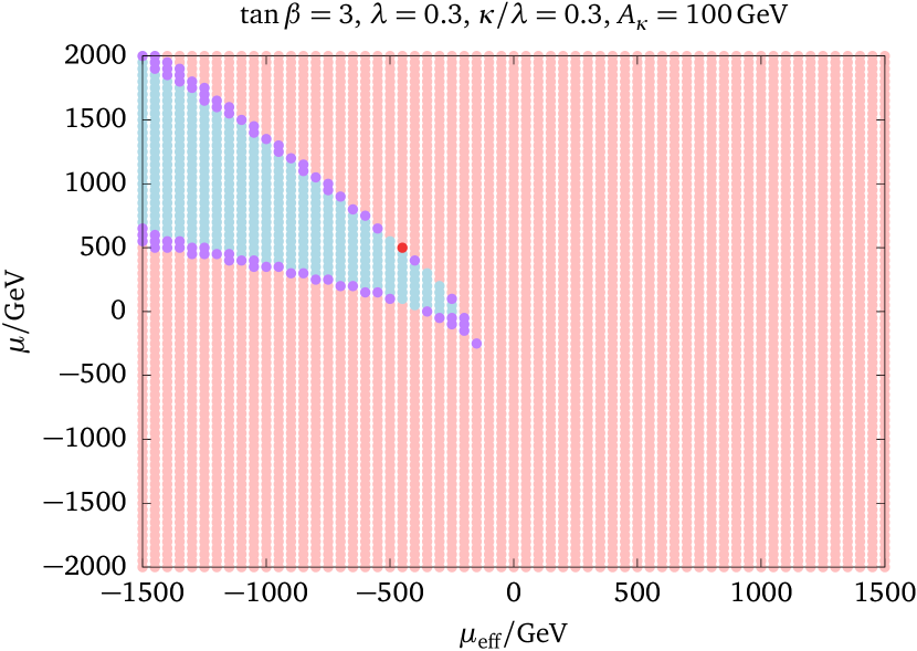
Figure 1: Mainly tachyonic constraints (pink points) confine the allowed parameter space (light blue). In addition, there exist other global minima than the electroweak vevs with a mostly long-lived desired vacuum (purple) and rarely short-lived configurations (red). On the left panel, $A_{\kappa}$ is taken to be $0\,\mathrm{GeV}$, where on the right panel $A_{\kappa}=100\,\mathrm{GeV}$. The positive value of $A_{\kappa}$ disallows the right wing for positive $\mu_{\text{eff}}$ that was allowed for vanishing $A_{\kappa}$ (in this case, there is a reflection symmetry). Moreover, there is a clear correlation between the allowed signs of $\mu$ and $\mu_{\text{eff}}$, which in most cases have to differ unless $\mu$ appears to be small. The other sign of $A_{\kappa}$ reversed the situation.

The effect of both $\mu$ and $\mu_{\text{eff}}$ on the tachyonicity of states can be seen from the dependence of the Higgs spectra on these parameters. In Figure 2, we show the functional dependence of the two lightest scalar and the lightest pseudoscalar masses on $\mu_{\text{eff}}$ for several values of $\mu$. The heavy states are mainly dominated by the input $m_{H^{\pm}}=800\,\mathrm{GeV}$.

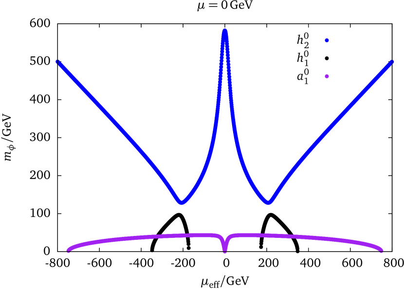
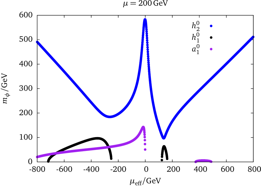
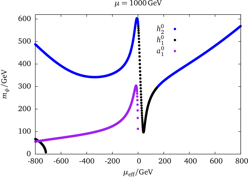
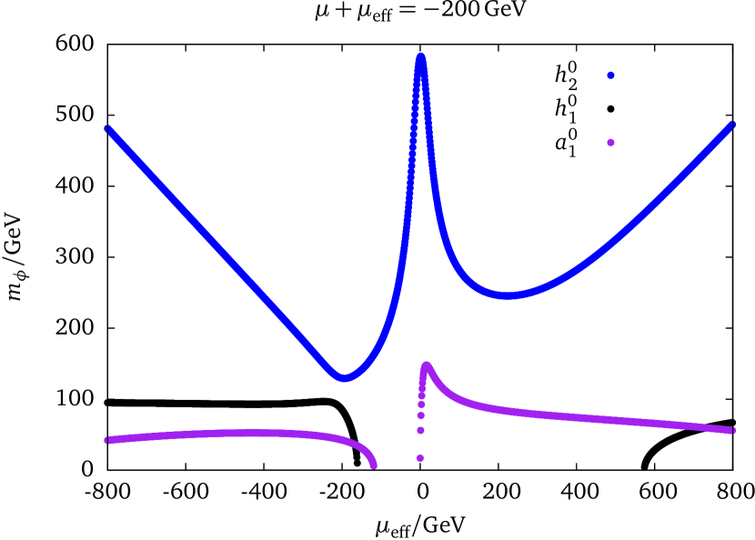
Figure 2: The spectra of the lightest states and how they vary with varying $\mu_{\text{eff}}$, exemplarily for some choice of parameters. In each plot, the $\mu$ value is fixed to a given value, where the lower right plot has a fixed sum $\mu+\mu_{\text{eff}}=-200\,\mathrm{GeV}$. It can be clearly seen which intervals are allowed (those with all three states appearing in the plot; where one or more are missing, these are tachyonic). In the case with $\mu=1000\,\mathrm{GeV}$ $h_{1}^{0}$ and $h_{2}^{0}$ apparently change their role which is due to the fact that the absolute value of the tachyonic state grows above the corresponding value of $h_{2}^{0}$. The scenario with $\mu=200\,\mathrm{GeV}$ shows the feature that the tachyonic exclusions are exclusive in the sense that one tachyonic state (scalar or pseudoscalar) is enough to exclude the spectrum. Here, both the lightest scalar and pseudoscalar have some small interval for positive $\mu_{\text{eff}}$ where they are non-tachyonic but the respective other one is and thus all the range for positive $\mu_{\text{eff}}$ is excluded (where $a_{1}^{0}$ turns tachyonic the first time for growing $\mu_{\text{eff}}$) and additionally already the light scalar mass gets tachyonic at larger negative values of $\mu_{\text{eff}}$. This artefact can be also seen in the region plot of Figure 1.

A precise knowledge of the Higgs sector in the NMSSM hence allows to distinguish between the pure $\mathds{Z}_{3}$-symmetric NMSSM and the inflation-inspired iNMSSM with the additional $\mathds{Z}_{3}$-breaking $\mu$-term. So far, we have not considered the additional soft SUSY breaking bilinear and kept it zero. In combination with a measurement of the neutralino sector, which in contrast rather mimics the NMSSM, there is a clear smoking gun of inflation that can be detected at an electroweak precision machine like a future Linear Collider. The Higgs spectrum varies severely with varying $\mu$ as we show in Figure 3. Here, we compare the light pseudoscalar case with vanishing $A_{\kappa}$ with the heavier scenario where $A_{\kappa}=100\,\mathrm{GeV}$ for illustrative reasons. While the light pseudoscalar mass is lifted up mainly by the amount of $A_{\kappa}$, the tachyonic state for $\mu=1000\,\mathrm{GeV}$ gets non-tachyonic and the scalar spectrum only changes marginally. The heavy states are merely fixed by the input value of the charged Higgs mass $m_{H^{\pm}}=800\,\mathrm{GeV}$.

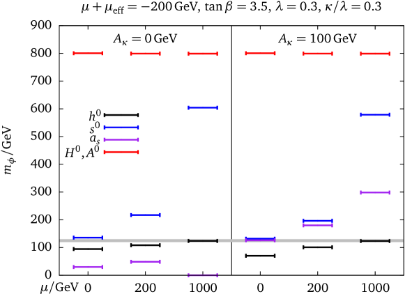
Figure 3: The Higgs spectra change with different choice of $\mu$ from $0$, $200$ to $1000\,\mathrm{GeV}$, where the black line corresponds to the SM-like state. The grey band around $125\,\mathrm{GeV}$ shows the experimentally favoured region with an error of $\pm 3\,\mathrm{GeV}$. The effective higgsino parameter was fixed to a value of $\mu+\mu_{\text{eff}}=-200\,\mathrm{GeV}$. On the right side, with respect to the left side, the $A_{\kappa}$ contribution is risen from $0$ to $100\,\mathrm{GeV}$ which lifts the pseudoscalar singlet mass of $a_{s}$ up and turns the tachyonic point at $A_{\kappa}=0\,\mathrm{GeV}$ and $\mu=1000\,\mathrm{GeV}$ non-tachyonic with a rather large $a_{s}$ mass.

The electroweakino sector is defined and briefly described in Appendix A, where it can be seen from the neutralino mass matrix that the singlino mass is governed by $\tfrac{\kappa}{\lambda}\mu_{\text{eff}}$, where the higgsino mass is determined by $\mu+\mu_{\text{eff}}$. Thus, a small higgsino mass, and therefore especially also a small charged higgsino mass, which is preferably detectable at a Linear Collider, is somewhat naturally selected in the iNMSSM where $\mu$ and $\mu_{\text{eff}}$ have to have opposite signs and rather the same magnitude. Such a cancellation, however, if $\mu$ is significantly large, tends to produce a heavy singlino in the iNMSSM in contrast to the NMSSM. This effect can be removed by adjusting the ratio $\kappa/\lambda$ in such a way that both singlino and higgsino masses scale the same with $\mu$. By this redefinition, however, if $\lambda$ is kept fixed, the value of $\kappa$ changes dramatically. While the electroweakino sector may look the same as in the NMSSM even in the presence of a large $\mu$-term, the (pseudo)scalar sector still has a strong dependence on the additional $\mu$-term which is shown in Figure 4.

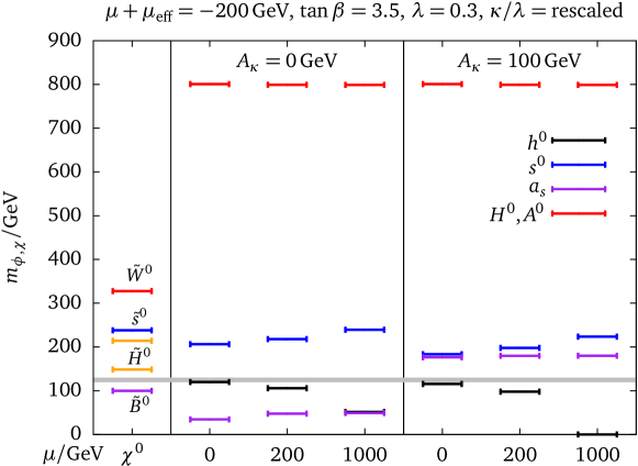
Figure 4: While the neutralino spectrum stays invariant under change of $\mu$, where the sum $\mu+\mu_{\text{eff}}=-200\,\mathrm{GeV}$ is fixed and the ratio $\kappa/\lambda$ rescaled in such a way to keep the singlino mass fixed as well, the scalar and pseudoscalar Higgs spectrum still change with varying $\mu$.

All the considerations and predictions presented above still depend on other, previously suppressed parameters. For the illustrative purpose, these additional parameters have been fixed to some values, variation of them also changes the structure of the plots shown in this talk. Especially the top/stop sector enters the determination of the SM-like Higgs mass, where we show mass contours in an interesting slice of parameter space in the following. The Higgs mass predictions contain the full iNMSSM one-loop and leading two-loop contributions, where the stop contribution in all cases was fixed to be sizeable and beyond the direct limits on stop searches in such a way that $m_{\tilde{t}}=2\,\mathrm{TeV}$ and the mixing was chosen to be $A_{t}=2m_{\tilde{t}}$. This particular choice, of course, can and has to be adjusted in a precision analysis. Moreover, the influence of the other input parameters as $\tan\beta$, $\lambda$, $\kappa$, and to some extend $A_{\kappa}$, still has to be tackled down in order to clearly determine the precision needed to distinguish two different scenarios of the NMSSM and the iNMSSM generating similar spectra. In addition, the electroweak phenomenology also involves production and decay rates of the Higgs states and thus one has an additional handle to distinguish the two models. In any case, a precise measurement of the electroweak sector at a future collider will give clear insights whether there is a smoking gun of inflation at the Linear Collider or not. This will be discussed in a forthcoming publication [11].

We have discussed above that an interesting slice of parameter space is defined by the sum of the two $\mu$-terms, $\mu+\mu_{\text{eff}}$, and the ratio $\kappa/\lambda$. The couplings $\lambda$ and $\kappa$ are known to run into a Landau pole below the GUT scale in the NMSSM, and the same is true for the iNMSSM since the additional $\mu$-term does not change the running. This non-perturbativity can be avoided, if $\lambda$ and $\kappa$ are taken to be constrained by $\lambda^{2}+\kappa^{2}\lesssim 0.5$, which will be always the case in the region plots shown in the following. The phenomenologically interesting regions are those where the SM-like Higgs state can accommodate for the observed $125\,\mathrm{GeV}$, the branching ratios are in those cases SM-like as well. There is an experimental exclusion from direct higgsino searches which constrains the chargino mass to be $\lesssim 94\,\mathrm{GeV}$; this bound approximately transfers to $\mu+\mu_{\text{eff}}$.

Parameter scans and results

The parameter space of the iNMSSM gets enlarged by two dimensions ($\mu$ and $B_{\mu}$) with respect to the NMSSM. Additionally, the new parameters may invalidate certain allowed regions of the NMSSM that become e. g. tachyonic once a sufficiently large $\mu$ parameter is turned on. On the other hand, as we have seen, there might be cancellations between $\mu$ and $\mu_{\text{eff}}$. The surviving parameter space appears to be rather constrained, which allows to have some clear predictions, especially on the hierarchy of Higgs boson masses. Unfortunately, as there are many parameters available, modification of one of these where the others remain fixed, relax the constraints and thus diminish the predictability. This, however, comes along with a different phenomenology and thus clearly distinguish different scenarios.

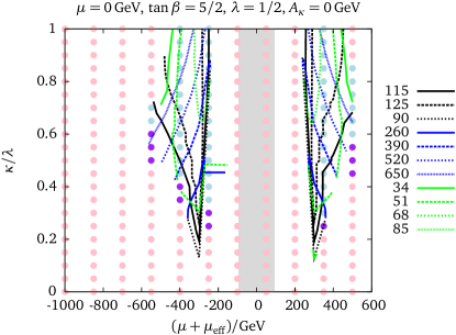
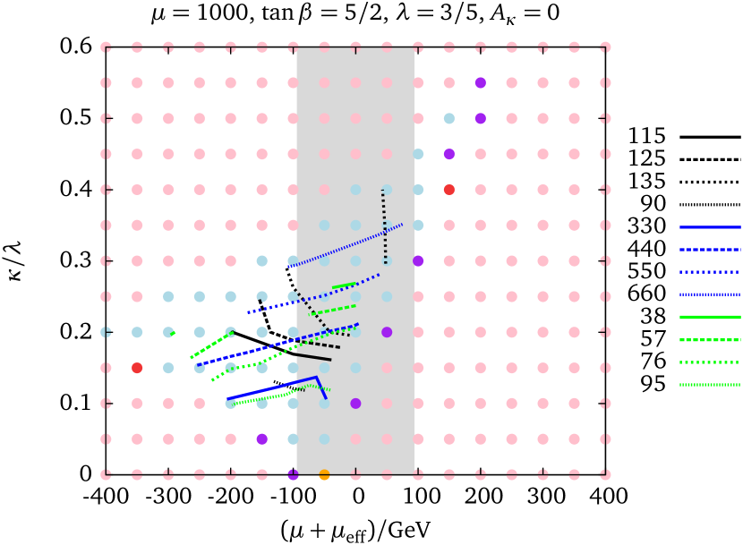
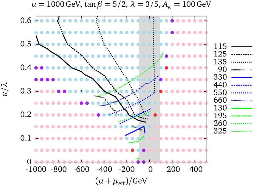
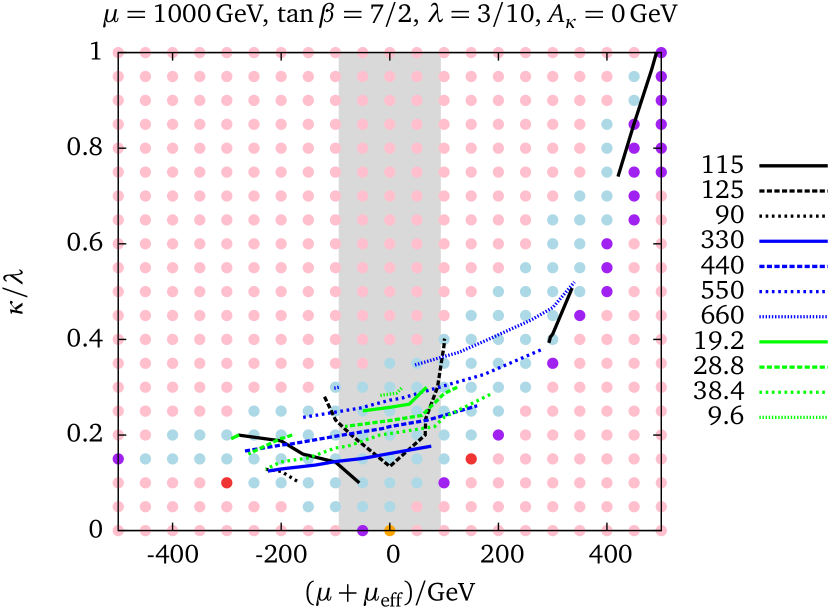
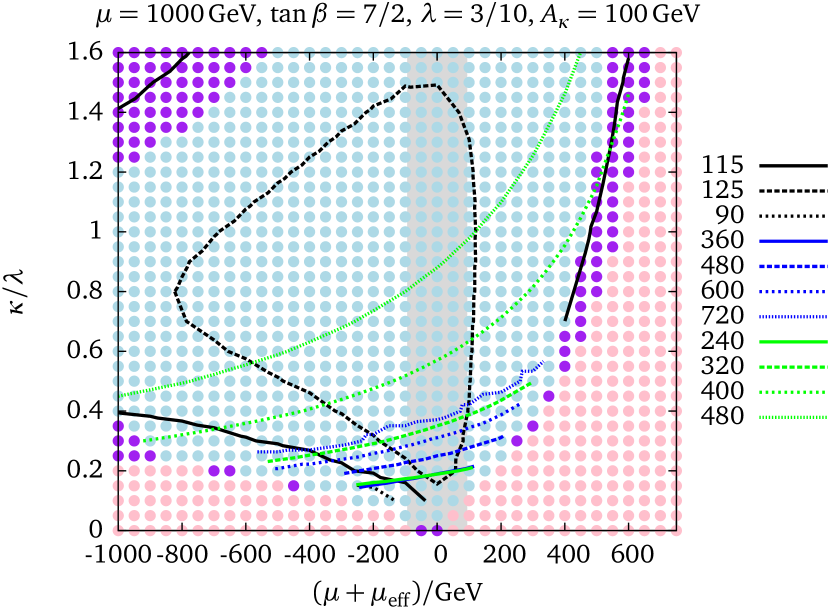
Figure 5: This selection shows some typical features of the iNMSSM and NMSSM. The upper plot has the situation with a vanishing $\mu$ and $A_{\kappa}$ which is symmetric around $\mu_{\text{eff}}=0\,\mathrm{GeV}$. The lower plots have a larger $\mu=1\,\mathrm{TeV}$ and show the effect of $A_{\kappa}$ on the allowed space and the Higgs masses. The contour lines give lines of equal masses for the SM-like Higgs (black), the singlet-like scalar (blue) and singlet-like pseudoscalar (green) which can be light for small $A_{\kappa}$. The colour code for the points describes the stability of the electroweak ground state: light blue points have a global electroweak vacuum, purple ones a long-lived and red points a short-lived desired vacuum. Tachyonic points are shown in pink, where the orange points do not fulfil the NMSSM constraint $A_{\kappa}^{2}>9m_{S}^{2}$ for a non-vanishing singlet vev.

One crucial parameter, as already discussed above, is given by $A_{\kappa}$ which controls the mass of the singlet pseudoscalar state. Low values of $A_{\kappa}$ produce a rather light state, heavier masses can be generated by lifting $A_{\kappa}$ up and simultaneously removing tachyons from the spectrum. There appears to be a larger fraction in the parameter space allowed, if one takes a look at the $\kappa/\lambda$ vs. $\mu+\mu_{\text{eff}}$ slice. This is shown in the samples of Figure 5. Comparing the cases with $A_{\kappa}=0$ and $100\,\mathrm{GeV}$, the effect of opening up excluded tachyonic parameter space can be clearly seen for the cost of a heavier singlet pseudoscalar (green contours). The other parameters only have a minor effect, so $\tan\beta$ is enhanced from $2.5$ to $3.5$ from the second to the third row of Figure 5 and simultaneously $\lambda$ reduced from $0.6$ to $0.3$, where $\mu=1\,\mathrm{TeV}$ in all cases. The single plot on top of Figure 5 illustrates the “NMSSM-limit” with vanishing $\mu$. Here, apparently only a very constrained region is allowed (note that $A_{\kappa}=0\,\mathrm{GeV}$) and the singlet-like pseudoscalar can be rather light. The grey bands show a rough experimental exclusion on the higgsino mass given by the LEP-limit on the chargino mass $m_{\chi^{\pm}_{1}}>94\,\mathrm{GeV}$ [12]. The chargino mass in the iNMSSM is mainly given by $\mu+\mu_{\text{eff}}$, see Appendix A, up to small modifications from the mixing.

Figure 5 also reveals information about the vacuum structure of the scanned points: light blue points denote an absolutely stable electroweak vacuum, where tachyonic states (at the tree-level!) appear in the pink points. Interestingly, the allowed regions can also easily accommodate for a $125\,\mathrm{GeV}$ SM-like Higgs state, where we added a uniform stop contribution as discussed above. Unstable or metastable desired vacua are coded in purple (long-lived) and red (short-lived). We briefly describe in Appendix B how we estimate the life-time. In the NMSSM there exists a bound on $A_{\kappa}$,

$$A_{\kappa}^{2}>9m_{S}^{2},$$ (18)

relating the trilinear soft SUSY breaking singlet coupling with the soft SUSY breaking singlet mass. This constraint is needed to generate a sufficiently large singlet vev and therefore higgsino mass. In the presence of the $\mathds{Z}_{3}$-breaking $\mu$-term, this unequation does not have to be necessarily fulfiled. Eq. (18) can be easily derived from the singlet-only potential with the requirement that the minimum $\langle S\rangle\neq 0$ is the true vacuum and thus a non-vanishing singlet vev is generated. This is needed in the $\mathds{Z}_{3}$-invariant NMSSM to produce the correct electroweak phenomenology. In the iNMSSM, however, the $\mathds{Z}_{3}$-breaking MSSM-like $\mu$-term is generated by the non-minimal coupling to supergravity and related to the scale of SUSY breaking and the gravitino mass. If both $\mu$ and $\mu_{\text{eff}}$ are present, there can be cancellations since they have to have different signs and hence a small higgsino mass still can be valid even if both $\mu$ parameters are in the $\mathrm{TeV}$ range.

Constraints on $B_{\mu}$

The iNMSSM has in addition to the superpotential parameter one more soft SUSY breaking term, the bilinear $B_{\mu}$-term, which has been ignored to far in the discussion above. It turns out that it cannot be arbitrarily large anyway and thus there are good reasons to keep it small. If it is non-zero, the effect is merely under control as the contribution from $B_{\mu}$ grows linearly with $\mu$ (note that it appears as $\mu B_{\mu}$ in the soft breaking potential). Together with $A_{\lambda}$ it influences the charged Higgs mass and therefore, in our approach where we treat $A_{\lambda}$ for $m_{H^{\pm}}$ as input, it enters the determination of $A_{\lambda}$, see Eq. (24) and Appendix A.

Unfortunately, the role of $B_{\mu}$ is less clear than compared to the MSSM where it can easily be replaced by the pseudoscalar mass $m_{A}$. However, its impact on the Higgs boson masses is very well-defined as it always enters in sum with $\mu_{\text{eff}}\tfrac{\kappa}{\lambda}$ and $\mu_{\text{eff}}A_{\lambda}$. Thus, it might be absorbed in $A_{\lambda}$, which nevertheless appears also at different places. Treating the charged Higgs mass $m_{H^{\pm}}$ as input and solving for $A_{\lambda}$, $\mu B_{\mu}$ enters the determination of $A_{\lambda}$. For too large values of $B_{\mu}$, tachyonic states are generated again. There is, however, a valley that allows for non-tachyonic states even for large but negative $B_{\mu}$ values as can be seen from Figure 6. It has nevertheless the power to destabilize the desired electroweak ground state of the theory as such large values of $B_{\mu}$ induce a global minimum different from the standard vacuum. The desired but local vacuum now appears to be rather short-lived with respect to the life-time of the universe, which is depicted by the red points of Figure 6. In the boundary region, the electroweak vacuum is sufficiently long-lived (purple points). The scalar singlet mass (blue lines) appears to be rather independent of $B_{\mu}$, where the pseudoscalar singlet (green) shows a striking behaviour depending on $A_{\kappa}$. The mass of the SM-like Higgs boson is very much aligned with the allowed valley and explains very well the tachyonic boundary (together with the pseudoscalar singlet as can be already seen from Figure 2, where $B_{\mu}=0\,\mathrm{GeV}$ but the two light states running tachyonic at different places).

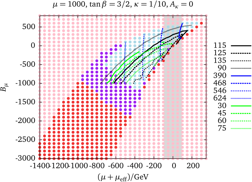
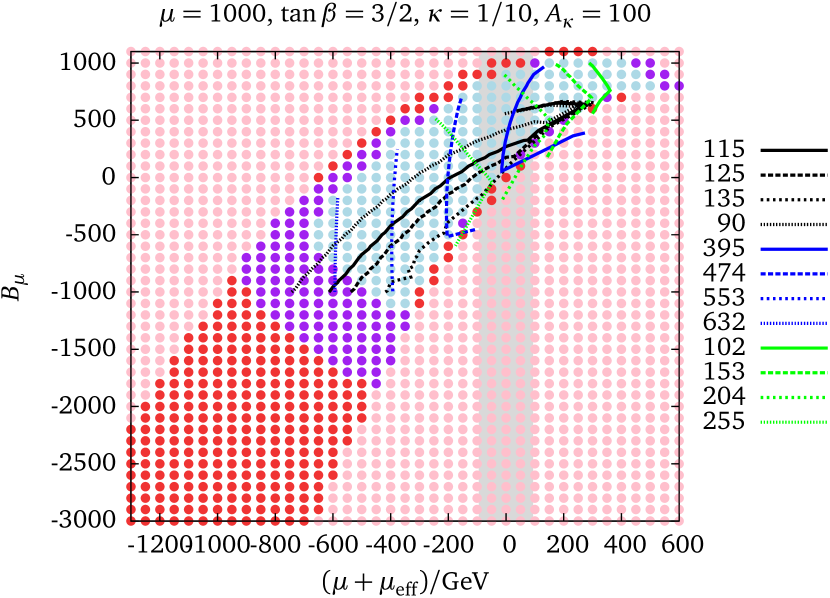
Figure 6: The color code of the points and lines is as in Figure 5. Now we show for fixed values of $\kappa=0.1$ and $\lambda=0.5$ a different slice in parameter space for non-vanishing $B_{\mu}$. In this region, the influence from $A_{\kappa}$ is apparently very mild (left $A_{\kappa}=0\,\mathrm{GeV}$, right $A_{\kappa}=100\,\mathrm{GeV}$). For too large negative values of $B_{\mu}$, the electroweak vacuum gets severely short-lived (red points) with a broad band of long-lived desired vacua in between (purple).

4 Conclusions

We have presented the electroweak phenomenology of an inflation-inspired NMSSM as first discussed in Refs. [1, 2, 3]. We briefly summarized the idea of Higgs inflation in the superconformal sector and showed how the non-minimal coupling of the Higgs sector to supergravity shows up in the effective low-energy superpotential. The remaining model can be described by the NMSSM augmented with an MSSM-like $\mu$-term $\mu\;H_{u}\cdot H_{d}$, which breaks the accidental $\mathds{Z}_{3}$ invariance of the NMSSM. Additionally, a soft SUSY breaking term $\mu B_{\mu}$ is generated and has to be taken into account. The rules of supergravity dictate $\mu$ and together with the effective $\mu$-term of the NMSSM arising from the singlet vev, both sum up to an effective higgsino mass $\mu+\mu_{\text{eff}}$. This combination plays an important role for the phenomenology, especially since the signs of both contributions appear to be anticorrelated and thus a natural cancellation among those fundamentally different contributions to the higgsino mass appears. Thus, scenarios with light higgsinos but heavy singlinos exist and a precise knowledge of the Higgs and electroweakino sector as it might be achieved at a future Linear Collider helps to clearly distinguish this model from the ordinary NMSSM. A smoking gun of the inflationary remnant exists as a footprint in the electroweak spectrum.

We have extensively discussed the influence of the model parameters on the Higgs masses and how tachyonic states are generated at the tree-level. Tachyonic masses invalidate the expansion point in such a way that the electroweak point appears to be a local maximum instead of a minimum and thus the tachyonic direction points towards the global minimum. In addition, the iNMSSM as well as the NMSSM may reveal several vacua out of which the desired vacuum appears to be a false vacuum. A numerical analysis minimising the scalar potential finds the global minimum of the theory, which in some cases is the electroweak vacuum in others not. If the desired vacuum is a local minimum, vacuum decay rates have been estimated to compare the life-time of the false vacuum with the life-time of the universe. Only in the case of large and negative $B_{\mu}$ values, reasonable amounts of short-lived vacua have been found.

Higgs inflation embedded into a superconformal framework appears to be distinguishable at low energies from the common SUSY models beyond the SM. The iNMSSM needs an additional singlet as the NMSSM; the spectrum, however, appears to be different and cannot be matched to the parameters of the NMSSM. The model is also different from the MSSM, in which Higgs inflation cannot be accommodated.

The results presented in this talk are going to be discussed in more detail in a forthcoming publication [11].

Appendix A Higgs boson and neutralino/chargino mass matrices

We define the Higgs mass matrices via the second derivatives of the potential, where we distinguish between scalar and pseudoscalar neutral states by the decomposition

$$H_{u} =\begin{pmatrix}H_{u}^{+}\\ H_{u}^{0}\end{pmatrix}=\begin{pmatrix}\phi^{+}_{u}\\ v_{u}+\tfrac{1}{\sqrt{2}}\left(\sigma_{u}+\mathrm{i}\,\phi_{d}\right)\end{pmatrix},\qquad H_{u}=\begin{pmatrix}H_{d}^{0}\\ H_{d}^{-}\end{pmatrix}=\begin{pmatrix}v_{d}+\tfrac{1}{\sqrt{2}}\left(\sigma_{d}+\mathrm{i}\,\phi_{d}\right)\\ \phi_{d}^{-}\end{pmatrix},$$ (19)

$$S =v_{s}+\tfrac{1}{\sqrt{2}}\left(\sigma_{s}+\mathrm{i}\,\phi_{s}\right).$$

The mass matrices for the scalar and pseudoscalar states $\mathcal{M}^{2}_{S}$ and $\mathcal{M}^{2}_{P}$, respectively, are then given by the expressions

$$\mathcal{M}^{2}_{S} =\begin{pmatrix}M_{Z}^{2}c_{\beta}^{2}+a_{1}t_{\beta}&\left(2v^{2}\lambda^{2}-M_{Z}^{2}\right)c_{\beta}s_{\beta}-a_{1}&a_{2}c_{\beta}-a_{3}s_{\beta}\\ *&M_{Z}^{2}s_{\beta}^{2}+a_{1}/t_{\beta}&a_{2}s_{\beta}-a_{3}c_{\beta}\\ *&*&a_{4}+a_{5}\end{pmatrix},$$ (20a)

$$\mathcal{M}^{2}_{P} =\begin{pmatrix}a_{1}t_{\beta}&a_{1}&-a_{6}s_{\beta}\\ *&a_{1}/t_{\beta}&-a_{6}c_{\beta}\\ *&*&a_{4}-3a_{5}-2a_{7}\end{pmatrix},$$ (20b)

with $s_{\beta}=\sin\beta$, $c_{\beta}=\cos\beta$, $t_{\beta}=\tan\beta$ and where the abbreviations $a_{i}$ are

$$a_{1} =B_{\mu}\mu+\mu_{\text{eff}}\left(\frac{\kappa}{\lambda}\mu_{\text{eff}}+A_{\lambda}\right),$$ (21a)

$$a_{2} =2v\lambda\left(\mu+\mu_{\text{eff}}\right),$$ (21b)

$$a_{3} =v\lambda\left(2\frac{\kappa}{\lambda}\mu_{\text{eff}}+A_{\lambda}\right),$$ (21c)

$$a_{4} =\frac{1}{\mu_{\text{eff}}}\left[v^{2}\lambda^{2}c_{\beta}s_{\beta}\left(\frac{\kappa}{\lambda}\mu_{\text{eff}}+A_{\lambda}\right)-v^{2}\lambda^{2}\mu\right],$$ (21d)

$$a_{5} =4\left(\frac{\kappa}{\lambda}\right)^{2}\mu_{\text{eff}}^{2}+\frac{\kappa}{\lambda}\left[\mu_{\text{eff}}\,A_{\kappa}-v^{2}\lambda^{2}c_{\beta}s_{\beta}\right],$$ (21e)

$$a_{6} =v\lambda\left(2\frac{\kappa}{\lambda}\mu_{\text{eff}}-A_{\lambda}\right),$$ (21f)

$$a_{7} =-6\left(\frac{\kappa}{\lambda}\right)^{2}\mu_{\text{eff}}^{2}\;.$$ (21g)

Note, that the pseudoscalar mass matrix comprises one massless state, the Goldstone mode. The charged Higgs mass matrix is given by

$$\mathcal{M}^{2}_{C}=\left[\left(M_{W}^{2}-v^{2}\lambda^{2}\right)c_{\beta}s_{\beta}+a_{1}\right]\begin{pmatrix}t_{\beta}&1\\ 1&1/t_{\beta}\end{pmatrix},$$ (22)

with the $W$ boson mass $M_{W}^{2}=\tfrac{1}{2}g_{2}^{2}v^{2}$ and the eigenvalue given by

$$m_{H^{\pm}}=M_{W}^{2}-v^{2}\lambda^{2}+\frac{a_{1}}{c_{\beta}s_{\beta}},$$ (23)

which can be used to eliminate $A_{\lambda}$ as a free parameter for the sake of the charged Higgs boson mass $m_{H^{\pm}}$ as input value (for the numerical analyses presented in this talk, we used allover the scenarios $m_{H^{\pm}}=800\,\mathrm{GeV}$), such that

$$A_{\lambda}=\frac{c_{\beta}s_{\beta}}{\mu_{\text{eff}}}\left(m_{H^{\pm}}^{2}-M_{W}^{2}+v^{2}\lambda^{2}\right)-\frac{B_{\mu}\mu}{\mu_{\text{eff}}}-\mu_{\text{eff}}\frac{\kappa}{\lambda}.$$ (24)

The mass matrices of charginos and neutralinos resemble very much the ordinary NMSSM, where the effective higgsino parameter is replaced by $\mu+\mu_{\text{eff}}$. However, the singlino mass is only governed by $\mu_{\text{eff}}$, since the additional $\mu$ term couples the doublet superfields. Therefore, the neutralino mass matrix is given by

$$\mathcal{M}_{\chi^{0}}=\begin{pmatrix}M_{1}&0&-M_{Z}s_{w}c_{\beta}&M_{Z}s_{w}s_{\beta}&0\\ *&M_{2}&M_{Z}c_{w}c_{\beta}&-M_{Z}c_{w}s_{\beta}&0\\ *&*&0&-(\mu+\mu_{\text{eff}})&-\lambda vs_{\beta}\\ *&*&*&0&-\lambda vc_{\beta}\\ *&*&*&*&2\tfrac{\kappa}{\lambda}\mu_{\text{eff}}\end{pmatrix},$$ (25)

where $M_{1}$ and $M_{2}$ are the gaugino masses for the $\mathrm{U}(1)_{Y}$ and $SU(2)_{L}$ gauginos, respectively, and the weak mixing angle $\theta_{w}$ enters via $\tan\theta_{w}=s_{w}/c_{w}=g_{1}/g_{2}$. Apparently, the neutralino spectrum in the iNMSSM can be rescaled via the ratio $\tfrac{\kappa}{\lambda}$ in such a way to match the NMSSM neutralino spectrum for a given higgsino mass $\mu+\mu_{\text{eff}}$.

The chargino mass matrix is given by

$$\mathcal{M}_{\chi^{\pm}}=\begin{pmatrix}M_{2}&\sqrt{2}M_{W}s_{\beta}\\ \sqrt{2}M_{W}c_{\beta}&\mu+\mu_{\text{eff}}\end{pmatrix}.$$ (26)

Appendix B Vacuum tunneling

We briefly describe our estimate on the tunneling rates in the case where the desired vacuum appears to be a false vacuum. The electroweak input parameters determine the position and depth of the local minimum, where the global minimum and true vacuum is found by numerical minimisation of the tree-level potential. In general, the true vacuum has vevs $\langle H^{0}_{u}\rangle\neq v_{u}$, $\langle H^{0}_{d}\rangle\neq v_{d}$ and $\langle S\rangle\neq v_{s}$. We approximate the potential barrier between the two minima by a one-dimensional quartic potential potential

$$V(\phi)=g\;\phi^{4}-a\;\phi^{3}+b\;\phi^{2}+c\;\phi+d,$$ (27)

which allows for an exact solution of the bounce action [13]. This is given by

$$B=\frac{\pi^{4}}{3g}(2-\delta)^{-3}\left[\alpha_{1}\delta+\alpha_{2}\delta^{2}+\alpha_{3}\delta^{3}\right],$$ (28)

with $\delta=8g^{2}b/a^{2}$ and $\alpha_{1,2,3}$ numerical coefficients. By comparison of the decay rate of the false vacuum per unit volume [14]

$$\Gamma/V=Ae^{-B/\hbar}\left[1+\mathcal{O}(\hbar)\right],$$ (29)

one estimates bounce actions $B\gtrsim 400$ to be sufficiently long-lived. The prefactor $A$ is difficult to calculate and usually approximated by the height of the potential or the electroweak scale, $A\sim(100\,\mathrm{GeV})^{4}$, where the error enters only logarithmically the decay time.

The interpolation between the two minima is done by a straight line, where the electroweak point is shifted to the origin. Therefore, in the expression of the neutral Higgs potential, we have the replacement

$$V(\phi)=V\left(H_{u}^{0}=v_{u}+(V_{u}-v_{u})\frac{\phi}{\sqrt{2}},H_{d}^{0}=v_{d}+(V_{d}-v_{d})\frac{\phi}{\sqrt{2}},S=v_{s}+(V_{s}-v_{s})\frac{\phi}{\sqrt{2}}\right),$$ (30)

with the “true” vevs $V_{u}$, $V_{d}$ and $V_{s}$. The factor $1/\sqrt{2}$ is employed to keep the $\phi$-field canonically normalised. This way, the field $\phi$ interpolates between the desired, false vacuum ($\phi=0$) and the true vacuum ($\phi=\sqrt{2}$). It is, however, more convenient to keep $\phi$ dimensionful and thus the coefficients of the potential in Eq. (27) of the same order of magnitude as the original coefficients. Therefore, we use a normalised field in the one-field potential, $V(\overline{\phi})$, with

$$\overline{\phi}=\frac{\phi}{\sqrt{(V_{u}-v_{u})^{2}/2+(V_{d}-v_{d})^{2}/2+(V_{s}-v_{s})^{2}/2}}.$$ (31)

References

- [1] M. B. Einhorn and D. R. T. Jones, “Inflation with Non-minimal Gravitational Couplings in Supergravity”, JHEP 03 (2010) 026, arXiv:0912.2718 [hep-ph].
- [2] S. Ferrara, R. Kallosh, A. Linde, A. Marrani, and A. Van Proeyen, “Jordan Frame Supergravity and Inflation in NMSSM”, Phys. Rev. D82 (2010) 045003, arXiv:1004.0712 [hep-th].
- [3] S. Ferrara, R. Kallosh, A. Linde, A. Marrani, and A. Van Proeyen, “Superconformal Symmetry, NMSSM, and Inflation”, Phys. Rev. D83 (2011) 025008, arXiv:1008.2942 [hep-th].
- [4] H. M. Lee, “Chaotic inflation in Jordan frame supergravity”, JCAP 1008 (2010) 003, arXiv:1005.2735 [hep-ph].
- [5] T. Moroi, H. Murayama, and M. Yamaguchi, “Cosmological constraints on the light stable gravitino”, Phys. Lett. B303 (1993) 289–294.
- [6] J. R. Ellis, J. E. Kim, and D. V. Nanopoulos, “Cosmological Gravitino Regeneration and Decay”, Phys. Lett. 145B (1984) 181–186.
- [7] U. Ellwanger, C. Hugonie, and A. M. Teixeira, “The Next-to-Minimal Supersymmetric Standard Model”, Phys.Rept. 496 (2010) 1–77, arXiv:0910.1785 [hep-ph].
- [8] G. G. Ross and K. Schmidt-Hoberg, “The Fine-Tuning of the Generalised NMSSM”, Nucl. Phys. B862 (2012) 710–719, arXiv:1108.1284 [hep-ph].
- [9] H. M. Lee, S. Raby, M. Ratz, G. G. Ross, R. Schieren, K. Schmidt-Hoberg, and P. K. S. Vaudrevange, “Discrete R symmetries for the MSSM and its singlet extensions”, Nucl. Phys. B850 (2011) 1–30, arXiv:1102.3595 [hep-ph].
- [10] A. Strumia, “Charge and color breaking minima and constraints on the MSSM parameters”, Nucl. Phys. B482 (1996) 24–38, arXiv:hep-ph/9604417 [hep-ph].
- [11] W. G. Hollik, S. Liebler, G. Moortgat-Pick, S. Paßehr, and G. Weiglein, “Phenomenology of the inflation-inspired NMSSM at the electroweak scale”, DESY-17-075, to be published.
- [12] Particle Data Group , C. Patrignani et al., “Review of Particle Physics”, Chin. Phys. C40 no. 10, (2016) 100001.
- [13] F. C. Adams, “General solutions for tunneling of scalar fields with quartic potentials”, Phys. Rev. D48 (1993) 2800–2805, arXiv:hep-ph/9302321 [hep-ph].
- [14] S. R. Coleman, “The Fate of the False Vacuum. 1. Semiclassical Theory”, Phys.Rev. D15 (1977) 2929–2936.