Weak mixing below the weak scale in dark-matter direct detection

Abstract

If dark matter couples predominantly to the axial-vector currents with heavy quarks, the leading contribution to dark-matter scattering on nuclei is either due to one-loop weak corrections or due to the heavy-quark axial charges of the nucleons. We calculate the effects of Higgs and weak gauge-boson exchanges for dark matter coupling to heavy-quark axial-vector currents in an effective theory below the weak scale. By explicit computation, we show that the leading-logarithmic QCD corrections are important, and thus resum them to all orders using the renormalization group.

I Introduction

A useful approach to describe the results of Dark Matter (DM) direct-detection experiments is to relate them to an Effective Field Theory (EFT) of DM coupling to quarks, gluons, leptons, and photons Bagnasco et al. (1994); Kurylov and Kamionkowski (2004); Kopp et al. (2010); Goodman et al. (2011, 2010); Bai et al. (2010); Hill and Solon (2012); Cirelli et al. (2013); Hill and Solon (2015); Crivellin et al. (2014); D’Eramo and Procura (2015); Hill and Solon (2014); Hoferichter et al. (2015); Bishara et al. (2017a); D’Eramo et al. (2016); Bishara et al. (2017b); D’Eramo et al. (2017). In this EFT, the level of suppression of DM interactions with the Standard Model (SM) depends on the mass dimension of the interaction operators, i.e., the higher the mass dimension the more suppressed the operator is. The mass dimension of operators is thus the organizing principle in capturing the phenomenologically most relevant effects, which is why in phenomenological analyses one keeps all relevant terms up to some mass dimension, $d$. An important question is, at which value of $d$ one can truncate the expansion. The obvious choice would be to keep all operators of dimension five and six, and a subset of dimension-seven operators that do not involve derivatives, as in this case one covers most of the UV models of DM.

In this work, we show that the leading contribution to the scattering cross section originates from double insertions of dimension-six operators if the DM interaction is predominantly due to DM vector currents coupling to heavy-quark axial-vector currents. This effectively means that in such a case it is necessary to extend the EFT to include operators of mass dimension eight. That such corrections are important was first pointed out in Refs. Crivellin et al. (2014); D’Eramo and Procura (2015), with the phenomenological implications further discussed in D’Eramo et al. (2017). We improve on the analysis of Ref. D’Eramo and Procura (2015) in two ways: i) we clarify how to consistently include the double-insertion contributions in the EFT framework, ii) we also perform the resummation of the QCD corrections at leading-logarithmic accuracy. Moreover, the generality of our approach covers also the case of non-singlet DM in the theory above the electroweak scale.

The paper is structured as follows. In Sections II–VI we derive our results for the case of Dirac-fermion DM. These are then extended to the case of Majorana-fermion DM and to the case of scalar DM in Section VII. In Section II we first show that the electroweak corrections have to be included if DM couples only to vector or axial-vector currents with heavy quarks. The weak interactions below the weak scale are encoded in an effective Lagrangian, which is introduced in Section III. Section IV contains our results for the anomalous dimensions controlling the operator mixing, while the renormalization-group evolution is given in Section V. In Section VI we show how our results connect to the physics above the electroweak scale. Section VIII contains conclusions, while Appendix A collects some unphysical operators entering in intermediate steps of our calculation.

II The importance of weak corrections for axial currents

We start by considering the DM EFT valid below the electroweak scale, $\mu_{b}<\mu<\mu_{\rm ew}$, for Dirac-fermion DM when five quark flavors are active,

$${\mathscr{L}}_{\chi}=\sum_{a,d}\frac{{\cal C}_{a}^{(d)}}{\Lambda^{d-4}}{\cal Q}_{a}^{(d)}\,.$$ (1)

The sums run over the dimensions of the operators, $d$, and the operator labels, $a$. The operators are multiplied by dimensionless Wilson coefficients, ${\cal C}_{a}^{(d)}$, and the appropriate powers of the mediator mass scale, $\Lambda$. Since we are interested in the theory below the electroweak scale, any interactions with the top quark, $W$, $Z$ bosons, and the Higgs are integrated out and are part of the Wilson coefficients ${\cal C}_{a}^{(d)}$. In this work, we focus on dimension-six operators, namely

$${\cal Q}_{1,f}^{(6)} =(\bar{\chi}\gamma_{\mu}\chi)(\bar{f}\gamma^{\mu}f)\,, {\cal Q}_{2,f}^{(6)} =(\bar{\chi}\gamma_{\mu}\gamma_{5}\chi)(\bar{f}\gamma^{\mu}f)\,,$$ (2)

$${\cal Q}_{3,f}^{(6)} =(\bar{\chi}\gamma_{\mu}\chi)(\bar{f}\gamma^{\mu}\gamma_{5}f)\,, {\cal Q}_{4,f}^{(6)} =(\bar{\chi}\gamma_{\mu}\gamma_{5}\chi)(\bar{f}\gamma^{\mu}\gamma_{5}f)\,,$$ (3)

where $f$ can be any of the SM fermions apart from the top quark. Our dimension counting follows Refs. Bishara et al. (2017b, c), such that scalar four-fermion operators are considered to be dimension seven, i.e., we assume they originate from a Higgs field insertion above the electroweak scale.

As we show below, a proper description of DM scattering on nuclei due to dimension-six operators requires including corrections from QED and the weak interactions. By contrast, such corrections are always subleading for dimension-five and dimension-seven operators. The basis of dimension-five operators, which couple DM to photons, can be found, e.g., in Refs. Bishara et al. (2017b, c), while the full basis of dimension-seven operators was derived in Ref. Brod et al. (2017).

If only a single operator in Eqs. (2)–(3) contributes, the cross section for DM–nucleus scattering can be written as

$$\sigma\propto\left(\frac{{\cal C}_{a}^{(d)}}{\Lambda^{d-4}}{\cal A}[{\cal Q}_{a}^{(d)}]\right)^{2},$$ (4)

where ${\cal A}[{\cal Q}_{a}^{(d)}]$ is an “effective scattering amplitude”. It is a product of the scattering amplitude, the nuclear response functions Fitzpatrick et al. (2013, 2012); Anand et al. (2014); Hoferichter et al. (2015, 2016); Bishara et al. (2017a), and all the relevant kinematic factors. We estimate ${\cal A}[{\cal Q}_{a}^{(d)}]$ in three different limits: i) in the limit of only strong interactions, ii) including QED corrections, and iii) also including corrections from weak interactions.

i) Switching off QED and weak interactions, the effective scattering amplitudes for dimension-six operators have the following parametric sizes (see Ref. Bishara et al. (2017c)):

$${\cal A}[{\cal Q}_{1,u(d)}^{(6)}] \sim A\,, {\cal A}[{\cal Q}_{1,s}^{(6)}] =0\,, {\cal A}[{\cal Q}_{1,c(b)}^{(6)}] =0\,,$$ (5)

$${\cal A}[{\cal Q}_{2,u(d)}^{(6)}] \sim{\rm max}\left\{v_{T}A,\frac{q}{m_{N}}\right\}\,, {\cal A}[{\cal Q}_{2,s}^{(6)}] =0\,, {\cal A}[{\cal Q}_{2,c(b)}^{(6)}] =0\,,$$ (6)

$${\cal A}[{\cal Q}_{3,u(d)}^{(6)}] \sim{\rm max}\left\{v_{T},\frac{q}{m_{\chi}}\right\}\,, {\cal A}[{\cal Q}_{3,s}^{(6)}] \sim\Delta s{\cal A}[{\cal Q}_{3,q}^{(6)}]\,, {\cal A}[{\cal Q}_{3,c(b)}^{(6)}] \sim\Delta c(b){\cal A}[{\cal Q}_{3,q}^{(6)}]\,,$$ (7)

$${\cal A}[{\cal Q}_{4,u(d)}^{(6)}] \sim 1\,, {\cal A}[{\cal Q}_{4,s}^{(6)}] \sim\Delta s{\cal A}[{\cal Q}_{4,q}^{(6)}]\,, {\cal A}[{\cal Q}_{4,c(b)}^{(6)}] \sim\Delta c(b){\cal A}[{\cal Q}_{4,q}^{(6)}]\,,$$ (8)

where in the subscript $q=u,d$. Here, $v_{T}\sim 10^{-3}$ is the typical DM velocity in the laboratory frame, $q$ is the typical momentum exchange, $q/m_{N}\lesssim 0.1$, where $m_{N}$ is the nucleon mass, and $A$ is the nuclear mass number (for heavy nuclei $A\sim 10^{2}$). The approximate expressions for the effective scattering amplitudes in Eqs. (5)–(8) include the parametric ${\mathcal{O}}(A)$ coherent enhancement of the spin-independent nuclear response function, $W_{M}(q)$, while all the other response functions were counted as ${\mathcal{O}}(1)$. The vector and axial form factors at zero recoil are ${\mathcal{O}}(1)$ for $u,d$ quarks. For the strange, charm and bottom quarks the vector form factors vanish. The axial charge for the strange quark is reasonably well known, $\Delta s=-0.031(5)$ Bishara et al. (2017b); Bali et al. (2012); Engelhardt (2012); Bhattacharya et al. (2014); Alexandrou et al. (2017). The axial charges of charm and bottom quarks currently have a much larger uncertainty. Ref. Polyakov et al. (1999) obtained $\Delta c\approx-5\cdot 10^{-4}$, $\Delta b\approx-5\cdot 10^{-5}$, with probably at least a factor of two uncertainty on these estimates.

Due to the non-relativistic nature of the problem and the sizes of the nuclear matrix elements, there are large hierarchies between the effective scattering amplitudes. For light quarks this hierarchy can be as large as $v_{T}/A\sim 10^{-5}$. For heavy quarks the effective amplitudes either vanish or are very small. This indicates that subleading corrections from QED and weak interactions may be important.

Figure 1: Photon penguin diagrams that induce mixing of DM vector interactions with leptons or heavy quarks into DM vector interactions with light quarks. Here, $f=u,d,s,c,b,e,\mu,\tau$ can denote any of the quarks or charged leptons.

ii) We now switch on corrections due to QED interactions. The diagrams with a closed fermion loop and a photon exchange, see Fig. 1, generate couplings to light quarks for all DM interactions with quark and lepton vector currents. The parametric estimates in Eqs. (5)–(6) are therefore modified to

$${\cal A}[{\cal Q}_{1,u(d)}^{(6)}] \sim A\,, {\cal A}[{\cal Q}_{1,s}^{(6)}] \sim\frac{\alpha}{4\pi}{\cal A}[{\cal Q}_{1,q}^{(6)}]\,, {\cal A}[{\cal Q}_{1,c(b)}^{(6)}] \sim\frac{\alpha}{4\pi}{\cal A}[{\cal Q}_{1,q}^{(6)}]\,,$$ (9)

$${\cal A}[{\cal Q}_{2,u(d)}^{(6)}] \sim{\rm max}\left\{v_{T}A,\frac{q}{m_{N}}\right\}\,, {\cal A}[{\cal Q}_{2,s}^{(6)}] \sim\frac{\alpha}{4\pi}{\cal A}[{\cal Q}_{2,q}^{(6)}]\,, {\cal A}[{\cal Q}_{2,c(b)}^{(6)}] \sim\frac{\alpha}{4\pi}{\cal A}[{\cal Q}_{2,q}^{(6)}],$$ (10)

while the parametric estimates for the operators with quark axial-vector currents, i.e., Eqs. (7)–(8), are not modified by the presence of QED corrections.

iii) Potentially important corrections to the effective amplitudes for operators with heavy-quark axial currents in Eqs. (7)–(8) are induced once weak interactions are included. Below the weak scale the $W$ and $Z$ bosons are integrated out, generating an effective weak Lagrangian ${{\mathscr{L}}}_{\text{eff}}^{\rm SM}$ composed of dimension-six four-fermion operators, see Eq. (12) in the next section. A double insertion of one four-fermion operator from ${{\mathscr{L}}}_{\text{eff}}^{\rm SM}$ and one from ${\mathscr{L}}_{\chi}$, see Fig. 2, induces the additional contributions to

$${\cal A}[{\cal Q}_{3,c(b)}^{(6)}]\sim\frac{\alpha}{4\pi s_{w}^{2}}\frac{m_{c(b)}^{2}}{m_{Z}^{2}}A\,,\qquad{\cal A}[{\cal Q}_{4,c(b)}^{(6)}]\sim\frac{\alpha}{4\pi s_{w}^{2}}\frac{m_{c(b)}^{2}}{m_{Z}^{2}}{\rm max}\left\{v_{T}A,\frac{q}{m_{N}}\right\}\,,$$ (11)

where $s_{w}$ is the sine of the weak mixing angle. The proportionality to the square of the heavy-quark mass $m_{c(b)}$ — necessary for dimensional reasons — can be deduced from the fact that it is the only relevant mass scale in the regime $\mu_{c(b)}<\mu<\mu_{\rm ew}$. For ${\cal Q}_{3,c(b)}^{(6)}$ these contributions dominate over the axial charge contribution, Eq. (7), by several orders of magnitude, while for ${\cal Q}_{4,c(b)}^{(6)}$ the electroweak corrections are either comparable or smaller than in Eq. (8). More details follow in the next sections.

The above estimates show that QED and weak corrections are essential to capture the leading contributions for the dimension-six operators in Eqs. (2)–(3) that involve heavy quarks. The same type of QED and weak radiative corrections also induce the leading effective amplitudes for the scattering on nucleons when the DM couples, at tree level, only to leptons. The logarithmically enhanced QED contributions are known, see for instance Refs. Hill and Solon (2015); D’Eramo and Procura (2015); Bishara et al. (2017c). In the present work, we calculate the logarithmically enhanced contributions due to the weak interactions. They arise, via double insertions, at second order in the dimension-six effective interactions, cf. Eq. (11). Accordingly, they can mix into dimension-eight operators, which, therefore, also have to be included.

It turns out that the weak corrections are numerically irrelevant for operators coupling DM to light quarks at tree level. Since the weak interactions do not conserve parity, they can lift the velocity suppression in the matrix elements of $Q_{3,q}^{(6)}$ through the mixing into the coherently enhanced operator $Q_{1,q}^{(6)}$. However, the resulting relative enhancement of order $A/v_{T}\sim 10^{5}$ is not enough to compensate for the large suppression of the weak corrections, of order $\alpha/(4\pi s_{w}^{2})(m_{q}/m_{Z})^{2}\lesssim 10^{-9}(m_{q}/100{\rm\leavevmode\nobreak\ MeV})^{2}$.

The weak corrections are also much less important for the dimension-five and dimension-seven operators coupling DM to the SM fields Bishara et al. (2017c); Brod et al. (2017). Most of these operators have a nonzero nucleon matrix element already without including electroweak corrections, in which case the latter only give subleading corrections. This is the case for the operators coupling DM to gluons or photons, for pseudoscalar currents with light quarks, and for scalar quark currents, including the ones with heavy bottom and charm quarks. In the special case where DM couples only to pseudoscalar heavy-quark currents the nuclear matrix elements vanish. This remains true also after one-loop electroweak corrections are included.

In the next two sections, we will obtain the leading-logarithmic expressions for the electroweak contributions in Eq. (11) and also resum the QCD corrections by performing the RG running from the weak scale, $\mu_{\rm ew}\sim{\mathcal{O}}(m_{Z})$, to the hadronic scale, $\mu_{\rm had}\sim{\mathcal{O}}(2{\rm\leavevmode\nobreak\ GeV})$, where we match to the nonrelativistic theory.

III Standard Model weak effective Lagrangian

The SM interactions below the weak scale are described by an effective Lagrangian, obtained by integrating out the top quark and the $Z$, $W$, and Higgs bosons at the scale $\mu_{\rm ew}\sim m_{Z}$. In this section we focus on quark interactions. We discuss leptons in Section VI. We can neglect any operators involving flavor-changing neutral currents as well as terms suppressed by off-diagonal Cabibbo–Kobayashi–Maskawa (CKM) matrix elements. The only necessary operators are

$$\begin{split}{{\mathscr{L}}}_{\text{eff}}^{\rm SM}\supset-\sqrt{2}G_{F}\,\bigg{\{}&\sum_{q\neq q^{\prime}}\bigg{[}\frac{1}{2}\sum_{i=1,2,4,5}{\cal D}_{i,qq^{\prime}}^{(6)}{\cal O}_{i,qq^{\prime}}^{(6)}+\sum_{i=3,6}{\cal D}_{i,qq^{\prime}}^{(6)}{\cal O}_{i,qq^{\prime}}^{(6)}\bigg{]}+\sum_{q}\!\!\sum_{i=1,\ldots,4}{\cal D}_{i,q}^{(6)}{\cal O}_{i,q}^{(6)}\bigg{\}}\,,\end{split}$$ (12)

where $G_{F}$ is the Fermi constant and ${\cal D}_{a}^{(6)}$ are dimensionless Wilson coefficients. The sums run over all light quarks, $q,q^{\prime}=u,d,s,c,b$, and the labels of the operators with two different quark flavors ($q\neq q^{\prime}$)

$${\cal O}_{1,qq^{\prime}}^{(6)} =(\bar{q}\gamma_{\mu}q)\,(\bar{q}^{\prime}\gamma^{\mu}q^{\prime})\,, {\cal O}_{2,qq^{\prime}}^{(6)} =(\bar{q}\gamma_{\mu}\gamma_{5}q)\,(\bar{q}^{\prime}\gamma^{\mu}\gamma_{5}q^{\prime})\,,$$ (13)

$${\cal O}_{3,qq^{\prime}}^{(6)} =(\bar{q}\gamma_{\mu}\gamma_{5}q)\,(\bar{q}^{\prime}\gamma^{\mu}q^{\prime})\,, {\cal O}_{4,qq^{\prime}}^{(6)} =(\bar{q}\gamma_{\mu}\,T^{a}q)\,(\bar{q}^{\prime}\gamma^{\mu}\,T^{a}q^{\prime})\,,$$ (14)

$${\cal O}_{5,qq^{\prime}}^{(6)} =(\bar{q}\gamma_{\mu}\gamma_{5}\,T^{a}q)\,(\bar{q}^{\prime}\gamma^{\mu}\gamma_{5}\,T^{a}q^{\prime})\,, {\cal O}_{6,qq^{\prime}}^{(6)} =(\bar{q}\gamma_{\mu}\gamma_{5}\,T^{a}q)\,(\bar{q}^{\prime}\gamma^{\mu}\,T^{a}q^{\prime})\,,$$ (15)

and a single quark flavor,

$${\cal O}_{1,q}^{(6)} =(\bar{q}\gamma_{\mu}q)\,(\bar{q}\gamma^{\mu}q)\,, {\cal O}_{2,q}^{(6)} =(\bar{q}\gamma_{\mu}\gamma_{5}q)\,(\bar{q}\gamma^{\mu}\gamma_{5}q)\,,$$ (16)

$${\cal O}_{3,q}^{(6)} =(\bar{q}\gamma_{\mu}\gamma_{5}q)\,(\bar{q}\gamma^{\mu}q)\,, {\cal O}_{4,q}^{(6)} =(\bar{q}\gamma_{\mu}\,T^{a}q)\,(\bar{q}\gamma^{\mu}\,T^{a}q)\,.$$ (17)

Here, $T^{a}$ are the $SU(3)_{c}$ generators normalised as ${\rm Tr}(T^{a}T^{b})=\frac{1}{2}\delta^{ab}$. As seen from the above operator basis, there are fewer linearly independent operators with a single quark than with two different quarks. The reason is that Fierz identities relate operators, like for instance the counterpart of ${\cal O}^{(6)}_{qq^{\prime}}$ with four equal quark fields, to the operators ${\cal O}_{i,q}^{(6)}$ with $i=1,\dots,4$. One way of implementing the Fierz relations is to project Green’s functions onto the basis that includes so-called Fierz-evanescent operators, like ${\cal E}_{7}^{q}$ and ${\cal E}_{8}^{q}$ in Eq. (87) of Appendix A, that vanish due to Fierz identities. SM operators with scalar or tensor currents do not contribute in our calculation. This is most easily seen by inspecting their chiral and Lorentz structure, neglecting operators with derivatives (see below).

Integrating out the $W$ and the $Z$ bosons at tree level gives the following values for the Wilson coefficients at $\mu_{\rm ew}$

$${\cal D}_{1,qq^{\prime}}^{(6)} =4s_{w}^{2}c_{w}^{2}v_{q}v_{q^{\prime}}+\frac{|I_{q}^{3}-I_{q^{\prime}}^{3}|}{6}|V_{qq^{\prime}}|^{2}\,, {\cal D}_{2,qq^{\prime}}^{(6)} =4s_{w}^{2}c_{w}^{2}a_{q}a_{q^{\prime}}+\frac{|I_{q}^{3}-I_{q^{\prime}}^{3}|}{6}|V_{qq^{\prime}}|^{2}\,,$$ (18)

$${\cal D}_{3,qq^{\prime}}^{(6)} =4s_{w}^{2}c_{w}^{2}a_{q}v_{q^{\prime}}-\frac{|I_{q}^{3}-I_{q^{\prime}}^{3}|}{6}|V_{qq^{\prime}}|^{2}\,, {\cal D}_{4,qq^{\prime}}^{(6)} ={\cal D}_{5,qq^{\prime}}^{(6)}=-{\cal D}_{6,qq^{\prime}}^{(6)}=|I_{q}^{3}-I_{q^{\prime}}^{3}||V_{qq^{\prime}}|^{2}\,,$$ (19)

and

$${\cal D}_{1,q}^{(6)}=2s_{w}^{2}c_{w}^{2}v_{q}^{2}\,, {\cal D}_{2,q}^{(6)}=2s_{w}^{2}c_{w}^{2}a_{q}^{2}\,, {\cal D}_{3,q}^{(6)}=4s_{w}^{2}c_{w}^{2}v_{q}a_{q}\,, {\cal D}_{4,q}^{(6)}=0\,.$$ (20)

Here, $s_{w}\equiv\sin\theta_{w}$, $c_{w}\equiv\cos\theta_{w}$, with $\theta_{w}$ the weak mixing angle, while $I_{q}^{3}$ is the third component of the weak isospin for the corresponding left-handed quark, i.e., $I_{q}^{3}=1/2$ for $q=u,c$ and $I_{q}^{3}=-1/2$ for $q=d,s,b$. The CKM matrix, $V_{qq^{\prime}}$, will be set to unity unless specified otherwise, while the vector and axial-vector couplings of the $Z$ boson to the quarks are encoded in

$$v_{q}\equiv\frac{I_{q}^{3}-2s_{w}^{2}Q_{q}}{2s_{w}c_{w}}\,, a_{q}\equiv-\frac{I_{q}^{3}}{2s_{w}c_{w}}\,,$$ (21)

where $Q_{q}$ is the electric charge of the corresponding quark. Note that ${\cal D}_{i,qq^{\prime}}^{(6)}\equiv{\cal D}_{i,q^{\prime}q}^{(6)}$ for $i=1,2,4,5$, since the corresponding operators are symmetric under $q\leftrightarrow q^{\prime}$.

IV Operator mixing and anomalous dimensions

Figure 2: A generic Feynman diagram with a double insertion of dimension-six operators, leading to the mixing into dimension-eight operators.

We are now ready to derive the leading contributions to the DM–nucleon scattering rates for the case that, at the weak scale, DM interacts with the visible sector only through the dimension-six operators ${\cal Q}_{3,q}^{(6)}$ or ${\cal Q}_{4,q}^{(6)}$, with $q=b,c$. To properly describe all the leading DM interactions we need to extend the dimension-six effective Lagrangian ${{\mathscr{L}}}_{\chi}$, Eq. (1), to include the following dimension-eight operators

$${{\mathscr{L}}}_{\chi}\supset-\frac{\sqrt{2}G_{F}}{\Lambda^{2}}\,\sum_{\begin{subarray}{c}q=u,d,s\\ i=1,\ldots,4\end{subarray}}{\cal C}_{i,q}^{(8)}{\cal Q}_{i,q}^{(8)}\,,$$ (22)

where

$${\cal Q}_{1,q}^{(8)} =\frac{m_{q}^{2}}{g_{s}^{2}}\,(\bar{\chi}\gamma_{\mu}\chi)(\bar{q}\gamma^{\mu}q)\,, {\cal Q}_{2,q}^{(8)} =\frac{m_{q}^{2}}{g_{s}^{2}}\,(\bar{\chi}\gamma_{\mu}\gamma_{5}\chi)(\bar{q}\gamma^{\mu}q)\,,$$ (23)

$${\cal Q}_{3,q}^{(8)} =\frac{m_{q}^{2}}{g_{s}^{2}}\,(\bar{\chi}\gamma_{\mu}\chi)(\bar{q}\gamma^{\mu}\gamma_{5}q)\,, {\cal Q}_{4,q}^{(8)} =\frac{m_{q}^{2}}{g_{s}^{2}}\,(\bar{\chi}\gamma_{\mu}\gamma_{5}\chi)(\bar{q}\gamma^{\mu}\gamma_{5}q)\,.$$ (24)

For future convenience, we defined the operators including two inverse powers of the strong coupling constant. Even if the Wilson coefficient of the dimension-eight operators are zero at $\mu_{\rm ew}$, they are generated below the electroweak scale from a double insertion of one of the dimension-six operators in ${{\mathscr{L}}}_{\chi}$ in Eq. (1) and one of the dimension-six operator from ${{\mathscr{L}}}_{\text{eff}}^{\rm SM}$ in Eq. (12), see Fig. 2. The logarithmic part of the running from $\mu_{\rm ew}$ to $\mu_{\rm had}$ gives

$$-\frac{\sqrt{2}G_{F}}{\Lambda^{2}}\frac{m_{q}^{2}}{g_{s}^{2}}{\cal C}_{1(2),q}^{(8)}(\mu_{\rm had}) \simeq\frac{\sqrt{2}G_{F}}{\Lambda^{2}}\frac{12}{\pi^{2}}a_{q}s_{w}^{2}c_{w}^{2}\sum_{q^{\prime}=c,b}m_{q^{\prime}}^{2}v_{q^{\prime}}{\cal C}_{3(4),q^{\prime}}^{(6)}(m_{Z})\log\Big{(}\frac{m_{q^{\prime}}}{m_{Z}}\Big{)},$$ (25)

where we set $\mu_{\rm ew}=m_{Z}$. This equation shows that the operators with derivatives, for instance, $(\bar{\chi}\gamma_{\mu}\chi)\partial^{2}(\bar{q}\gamma^{\mu}q)$, can be neglected because their effect on the scattering rates is not enhanced by the large ratio $m_{b,c}^{2}/m_{q}^{2}$. Furthermore, the set of operators in Eqs. (23)–(24) is closed under RG running up to mass-dimension eight, if we keep only terms proportional to two powers of the bottom- or charm-quark mass in the RG evolution. At higher orders in QCD the purely electroweak expression Eq. (25) gets corrected by terms of the order of $\alpha_{s}^{n-1}\log^{n}(m_{b(c)}/m_{Z})$. Since $m_{b(c)}\ll m_{Z}$, these terms can amount to ${\mathcal{O}}(1)$ corrections. In the following we resum these large QCD logarithms to leading-logarithmic order.

The techniques for the calculation of leading-logarithmic QCD corrections with double insertions are standard Witten (1977); Gilman and Wise (1983); Flynn (1990); Datta et al. (1990); Herrlich and Nierste (1995, 1996); Brod and Zupan (2014); Brod (2015). We first replace the bare Wilson coefficients in Eqs. (1), (12), and (22) with their renormalized counterparts. The corresponding effective Lagrangian reads

$$\begin{split}{{\mathscr{L}}}_{\text{eff}}=&\frac{1}{\Lambda^{2}}\sum_{a}{\cal C}_{a}^{(6)}{\cal Q}_{a}^{(6)}-\sqrt{2}G_{F}\sum_{ab}{\cal D}_{a}^{(6)}Z_{ab}{\cal O}_{b}^{(6)}\\ &-\frac{\sqrt{2}G_{F}}{\Lambda^{2}}\bigg{\{}\sum_{ab}{\cal C}_{a}^{(8)}\tilde{Z}_{ab}{\cal Q}_{b}^{(8)}+\sum_{abc}{\cal D}_{a}^{(6)}{\cal C}_{b}^{(6)}\hat{Z}_{ab,c}{\cal Q}_{c}^{(8)}\bigg{\}}\,.\end{split}$$ (26)

The compound indices $a$, $b$, $c$, run over both the operator labels and quark-flavor indices. In Eq. (26), we have already made use of the fact that the QCD anomalous dimensions of the operators ${\cal Q}_{a}^{(6)}$ in Eqs. (2)–(3) are zero, and have not introduced the corresponding renormalization constants.

In dimension regularization around $d=4-2\epsilon$ space-time dimensions, the renormalization constants admit a double expansion in the strong coupling constant and $\epsilon$

$$Z_{ab}=\delta_{ab}+\frac{\alpha_{s}}{4\pi}\sum_{k=0,1}\frac{1}{\epsilon^{k}}Z_{ab}^{(1,k)}+{\cal O}(\alpha_{s}^{2})\,,$$ (27)

and similarly for $\tilde{Z}$ and $\hat{Z}$.

The RG evolution of the dimension-six Wilson coefficients is determined by a RG equation that is linear in the Wilson coefficients,

$$\mu\frac{d}{d\mu}{\cal D}_{a}^{(6)}(\mu)=\sum_{b}{\cal D}_{b}^{(6)}(\mu)\gamma_{ba}\,,\qquad\text{with}\quad\gamma=-\frac{d\log Z}{d\log\mu}\,.$$ (28)

On the other hand, the running of the dimension-eight Wilson coefficients receives two contributions. In addition to the running of the $m_{q}^{2}/g_{s}^{2}$ prefactor, encoded in $\tilde{\gamma}$, there are contributions from double insertions of dimension-six operators, see Fig. 2. This leads to a RG equation that is quadratic in dimension-six Wilson coefficients Herrlich and Nierste (1995, 1996),

$$\mu\frac{d}{d\mu}{\cal C}_{a}^{(8)}(\mu)=\sum_{b}{\cal C}_{b}^{(8)}(\mu)\tilde{\gamma}_{ba}+\sum_{bc}{\cal D}_{b}^{(6)}(\mu){\cal C}_{c}^{(6)}(\mu)\hat{\gamma}_{bc,a}\,.$$ (29)

To leading order in the strong coupling constant the rank-three anomalous dimension tensor $\hat{\gamma}_{ab,c}$ Herrlich and Nierste (1995, 1996) is given by

$$\hat{\gamma}_{ab,c}=\frac{\alpha_{s}}{2\pi}\hat{Z}_{ab,c}^{(1,1)}+{\cal O}(\alpha_{s}^{2})\,.$$ (30)

Next we provide the explicit values for the anomalous dimensions. In our notation, the anomalous dimensions are expanded in powers of $\alpha_{s}$,

$$\gamma=\gamma^{(1)}+\gamma^{(2)}+\cdots\,,$$ (31)

with $\gamma^{(n)}\propto(\alpha_{s}/4\pi)^{n}$, and similarly for $\tilde{\gamma}$ and $\hat{\gamma}$.

We start by giving the results for the mixing of the dimension-eight operators coupling DM to quarks, Eqs. (23) and (24). This mixing is encoded in the $\tilde{\gamma}$ and $\hat{\gamma}$ anomalous dimensions. We obtain the $\hat{\gamma}$ from the poles of the double insertions, Fig. 2. The only nonzero entries leading to mixing into operators with light-quark currents are

$$\hat{\gamma}_{{\cal O}_{3,q^{\prime}q}^{(6)},{\cal Q}_{3,q^{\prime}}^{(6)};{\cal Q}_{1,q}^{(8)}}^{(1)}=\hat{\gamma}_{{\cal O}_{3,q^{\prime}q}^{(6)},{\cal Q}_{4,q^{\prime}}^{(6)};{\cal Q}_{2,q}^{(8)}}^{(1)}=\hat{\gamma}_{{\cal O}_{2,qq^{\prime}}^{(6)},{\cal Q}_{3,q^{\prime}}^{(6)};{\cal Q}_{3,q}^{(8)}}^{(1)}=\hat{\gamma}_{{\cal O}_{2,qq^{\prime}}^{(6)},{\cal Q}_{4,q^{\prime}}^{(6)};{\cal Q}_{4,q}^{(8)}}^{(1)}=-16N_{c}\frac{m_{q^{\prime}}^{2}}{m_{q}^{2}}\frac{\alpha_{s}}{4\pi}\,.$$ (32)

The remaining contribution to the RG running of the dimension-eight operators is entirely due to the $m_{q}^{2}/g_{s}^{2}$ prefactors in the definition of the operators, namely

$$\tilde{\gamma}_{ab}=2(\gamma_{m}^{(0)}-\beta_{0})\frac{\alpha_{s}}{4\pi}\delta_{ab}\,,\quad\text{where}\quad\gamma_{m}^{(0)}=6C_{F}\quad\text{and}\quad\beta_{0}=11-\frac{2}{3}N_{f}\,,$$ (33)

with $C_{F}=4/3$ for QCD, and $N_{f}$ the number of active quark flavors.

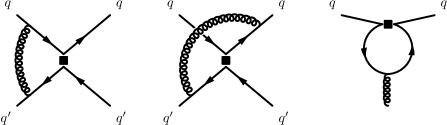
Figure 3: Selection of diagrams entering the computation of QCD one-loop anomalous dimension of four-fermion operators. The poles of QCD penguin diagrams affect the mixing via the e.o.m.-vanishing operators defined in Appendix A.

The RG running of the dimension-six operators in the SM weak effective Lagrangian is due to one-loop gluon exchange diagrams, see Fig. 3. Since the corresponding anomalous dimension matrix $\gamma$ has many entries, we split the result into several blocks.

The anomalous dimension matrix in the subsector spanned by the operators in Eqs. (16)–(17),

$$\big{(}{\cal O}_{1,q}^{(6)},\,{\cal O}_{2,q}^{(6)},\,{\cal O}_{3,q}^{(6)},\,{\cal O}_{4,q}^{(6)}\big{)}\,,$$ (34)

reads

$$\gamma^{(1)}=\frac{\alpha_{s}}{4\pi}\begin{pmatrix}4&4&0&-\frac{28}{3}\\ 0&0&0&\frac{44}{3}\\ 0&0&\frac{44}{9}&0\\ \frac{5}{3}&\frac{13}{3}&0&-\frac{106}{9}\end{pmatrix}.$$ (35)

Note that, at one-loop, there is no mixing into operators with a different quark flavor.

The anomalous dimensions describing the mixing of the same operators,

$$\big{(}{\cal O}_{1,q}^{(6)},\,{\cal O}_{2,q}^{(6)},\,{\cal O}_{3,q}^{(6)},\,{\cal O}_{4,q}^{(6)}\big{)}\,,$$ (36)

into the operators

$$\big{(}{\cal O}_{1,qq^{\prime}}^{(6)},\,{\cal O}_{2,qq^{\prime}}^{(6)},\,{\cal O}_{3,qq^{\prime}}^{(6)},\,{\cal O}_{3,q^{\prime}q}^{(6)},\,{\cal O}_{4,qq^{\prime}}^{(6)},\,{\cal O}_{5,qq^{\prime}}^{(6)},\,{\cal O}_{6,qq^{\prime}}^{(6)},\,{\cal O}_{6,q^{\prime}q}^{(6)}\big{)}\,,$$ (37)

read

$$\gamma^{(1)}=\frac{\alpha_{s}}{4\pi}\begin{pmatrix}0&0&0&0&\frac{8}{3}&0&0&0\\ 0&0&0&0&\frac{8}{3}&0&0&0\\ 0&0&0&0&0&0&\frac{8}{3}&0\\ 0&0&0&0&\frac{20}{9}&0&0&0\end{pmatrix}.$$ (38)

The anomalous dimension matrix in the subsector spanned by the operators in Eqs. (13)–(15),

$$\big{(}{\cal O}_{1,qq^{\prime}}^{(6)},\,{\cal O}_{2,qq^{\prime}}^{(6)},\,{\cal O}_{3,qq^{\prime}}^{(6)},\,{\cal O}_{3,q^{\prime}q}^{(6)},\,{\cal O}_{4,qq^{\prime}}^{(6)},\,{\cal O}_{5,qq^{\prime}}^{(6)},\,{\cal O}_{6,qq^{\prime}}^{(6)},\,{\cal O}_{6,q^{\prime}q}^{(6)}\big{)}\,,$$ (39)

reads

$$\gamma^{(1)}=\frac{\alpha_{s}}{4\pi}\begin{pmatrix}0&0&0&0&0&12&0&0\\ 0&0&0&0&12&0&0&0\\ 0&0&0&0&0&0&0&12\\ 0&0&0&0&0&0&12&0\\ 0&\frac{8}{3}&0&0&-\frac{19}{3}&5&0&0\\ \frac{8}{3}&0&0&0&5&-9&0&0\\ 0&0&0&\frac{8}{3}&0&0&-\frac{23}{3}&5\\ 0&0&\frac{8}{3}&0&0&0&5&-\frac{23}{3}\end{pmatrix}.$$ (40)

The part of the anomalous dimension matrix mixing the operators,

$$\big{(}{\cal O}_{1,qq^{\prime}}^{(6)},\,{\cal O}_{2,qq^{\prime}}^{(6)},\,{\cal O}_{3,qq^{\prime}}^{(6)},\,{\cal O}_{3,q^{\prime}q}^{(6)},\,{\cal O}_{4,qq^{\prime}}^{(6)},\,{\cal O}_{5,qq^{\prime}}^{(6)},\,{\cal O}_{6,qq^{\prime}}^{(6)},\,{\cal O}_{6,q^{\prime}q}^{(6)}\big{)}\,,$$ (41)

into the same operators, but with different quark flavor structure, $q^{\prime\prime}\neq q^{\prime}$,

$$\big{(}{\cal O}_{1,qq^{\prime\prime}}^{(6)},\,{\cal O}_{2,qq^{\prime\prime}}^{(6)},\,{\cal O}_{3,qq^{\prime\prime}}^{(6)},\,{\cal O}_{3,q^{\prime\prime}q}^{(6)},\,{\cal O}_{4,qq^{\prime\prime}}^{(6)},\,{\cal O}_{5,qq^{\prime\prime}}^{(6)},\,{\cal O}_{6,qq^{\prime\prime}}^{(6)},\,{\cal O}_{6,q^{\prime\prime}q}^{(6)}\big{)}\,,$$ (42)

is

$$\gamma^{(1)}=\frac{\alpha_{s}}{4\pi}\operatorname{diag}\Big{(}0,0,0,0,\frac{4}{3},0,\frac{4}{3},0\Big{)}.$$ (43)

Finally, the part of the anomalous dimension matrix mixing the operators

$$\big{(}{\cal O}_{1,qq^{\prime}}^{(6)},{\cal O}_{2,qq^{\prime}}^{(6)},{\cal O}_{3,qq^{\prime}}^{(6)},{\cal O}_{3,q^{\prime}q}^{(6)},{\cal O}_{4,qq^{\prime}}^{(6)},{\cal O}_{5,qq^{\prime}}^{(6)},{\cal O}_{6,qq^{\prime}}^{(6)},{\cal O}_{6,q^{\prime}q}^{(6)}\big{)}$$ (44)

into the operators

$$\big{(}{\cal O}_{1,q}^{(6)},{\cal O}_{2,q}^{(6)},{\cal O}_{3,q}^{(6)},{\cal O}_{4,q}^{(6)}\big{)}$$ (45)

has only two nonzero entries,

$$\gamma^{(1)}=\frac{\alpha_{s}}{4\pi}\begin{pmatrix}0&0&0&0\\ 0&0&0&0\\ 0&0&0&0\\ 0&0&0&0\\ 0&0&0&\frac{4}{3}\\ 0&0&0&0\\ 0&0&\frac{4}{9}&0\\ 0&0&0&0\end{pmatrix}.$$ (46)

All the remaining entries in $\gamma$ vanish. We extracted the anomalous dimensions from the off-shell renormalization of Green’s functions with appropriate external states. We checked explicitly that our results are gauge-parameter independent. In Appendix A, we list the evanescent and e.o.m.-vanishing operators that enter at intermediate stages of the computation.

V Renormalization Group evolution

With the anomalous dimensions of Section IV, we can now compute the Wilson coefficients at $\mu_{\rm had}\sim 2$ GeV in terms of initial conditions at the weak scale. The Wilson coefficients ${\cal C}_{b}^{(6)}$ do not run, thus ${\cal C}_{b}^{(6)}(\mu_{\rm had})={\cal C}_{b}^{(6)}(\mu_{\rm ew})$. The RG running for the remaining Wilson coefficients is controlled by the RG equations in Eqs. (28) and (29), which we combine into a single expression,

$$\mu\frac{d}{d\mu}\mathscr{C}_{a}(\mu)=\sum_{b}\mathscr{C}_{b}(\mu)\gamma_{ba}^{\text{eff}}\,.$$ (47)

Here, we defined a vector of Wilson coefficients as

$$\mathscr{C}(\mu)\equiv\begin{pmatrix}{\cal D}^{(6)}(\mu)\\ {\cal C}^{(8)}(\mu)\end{pmatrix}.$$ (48)

and absorbed the (scale-independent) Wilson coefficients ${\cal C}_{a}^{(6)}$ into the effective anomalous-dimension matrix

$$\gamma^{\text{eff}}\equiv\begin{pmatrix}\gamma&{\cal C}^{(6)}\cdot\hat{\gamma}\\ 0&\tilde{\gamma}\end{pmatrix}\qquad\text{with}\qquad({\cal C}^{(6)}\cdot\hat{\gamma})_{ba}\equiv\sum_{c}{\cal C}_{c}^{(6)}\hat{\gamma}_{bc,a}\,.$$ (49)

Since the ${\cal C}_{a}^{(6)}$ Wilson coefficients are RG invariant, the tensor product effectively transforms the rank-three tensor $\hat{\gamma}_{ab,c}$ into an equivalent matrix, ${\cal C}^{(6)}\cdot\hat{\gamma}$, with all its entries constant, that is equivalent to the tensor for the purpose of RG running. This has the advantage that one can use the standard methods for single insertions to solve the RG equations.

The RG evolution proceeds in multiple steps. The first step is the matching of the (complete or effective) theory of DM interactions above the weak scale onto the five-flavor EFT. This matching computation yields the initial conditions for ${\cal C}_{a}^{(6)}(\mu_{\rm ew})$ and ${\cal C}_{a}^{(8)}(\mu_{\rm ew})$ at the weak scale. At leading-logarithmic order it suffices to perform the matching at $\mu_{\rm ew}$ at tree-level. If the mediators have weak-scale masses, we obtain ${\cal C}_{a}^{(6)}(\mu_{\rm ew})\neq 0$ and ${\cal C}_{a}^{(8)}(\mu_{\rm ew})=0$. If the mediators are much heavier than the weak scale, with masses of order $M\gg m_{Z}$, the RG running above the electroweak scale can induce nonzero ${\cal C}_{a}^{(8)}(\mu_{\rm ew})\sim\log(\mu_{\rm ew}/M)$. We discuss the latter case in Section VI. For the RG evolution below the electroweak scale one also needs the coefficients ${\cal D}_{a}^{(6)}(\mu_{\rm ew})$. The SM contributions to the tree-level initial conditions for ${\cal D}_{a}^{(6)}(\mu_{\rm ew})$ are provided in Eqs. (18)–(20).

The second step is to evolve ${\cal C}_{a}^{(8)}(\mu)$ and ${\cal D}_{a}^{(6)}(\mu)$ from the electroweak scale to lower scales according to Eq. (47). The RG evolution is in a theory with $N_{f}=5$ quark flavors, when $\mu_{b}\leq\mu\leq\mu_{\rm ew}$, with $N_{f}=4$, when $\mu_{c}\leq\mu\leq\mu_{b}$, and with $N_{f}=3$, when $\mu_{\rm had}\leq\mu\leq\mu_{c}$. Here the $\mu_{b(c)}$ denote the threshold scale at which the bottom(charm)-quark is removed from the theory. In our numerical analysis we will use $\mu_{b}=4.18$ GeV and $\mu_{c}=2$ GeV. At leading-logarithmic order, there are no non-trivial matching corrections at the bottom- and charm-quark thresholds, and we simply have

$${\cal C}_{a}^{(d)}(\mu_{b})\big{|}_{N_{f}=4}={\cal C}_{a}^{(d)}(\mu_{b})\big{|}_{N_{f}=5}\,,\qquad\quad{\cal C}_{a}^{(d)}(\mu_{c})\big{|}_{N_{f}=3}={\cal C}_{a}^{(d)}(\mu_{c})\big{|}_{N_{f}=4}\,.$$ (50)

This means that we can switch to the EFT with four active quark flavors by simply dropping all operators in Eq. (26) that involve a bottom-quark field, and to the EFT with three active quark flavors by simply dropping all operators with charm-quark fields. The leading-order matching at $\mu_{q^{\prime}}\sim m_{q^{\prime}}$ comes with a small uncertainty due to the choice of matching scale that is of order $\log(\mu_{q^{\prime}}/m_{q^{\prime}})$. This is formally of higher order in the RG-improved perturbation theory. The uncertainty is canceled in a calculation at next-to-leading-logarithmic order by finite threshold corrections at the respective threshold scale.

This is a good point to pause and compare our results with the literature. The RG evolution of the operators in Eqs. (2)–(3) below the electroweak scale has been studied in Ref. D’Eramo and Procura (2015), which effectively resummed the large logarithms $\log(\mu_{\rm had}/\mu_{\rm ew})$ to all orders in the Yukawa couplings. Such a resummation is problematic for two reasons. Firstly, it does not take into account that the RG evolution stops at the heavy-quark thresholds, below which the Wilson coefficients are RG invariant. (Below the heavy-quark thresholds, there are no double insertions with heavy quarks and the running of the factor $m_{q}^{2}/g_{s}^{2}$ is precisely canceled by the running of the Wilson coefficients of the dimension-eight operators.) This introduces a spurious scale dependence of the Wilson coefficients in the three-flavor EFT, of the order of $|\log(\mu_{\rm had}/m_{b(c)})|\lesssim 50\%$, that is not canceled by the hadronic matrix elements. Secondly, such a resummation is not consistent within the EFT framework. Since there are no Higgs-boson exchanges in the EFT below the weak scale, the scheme-dependence of the anomalous dimensions and the residual matching scale dependence at the heavy-quark thresholds is not consistently canceled by higher-orders, leading to unphysical results.

Continuing with our analysis, the final step is to match the three-flavor EFT onto the EFT with nonrelativistic neutrons and protons that is then used to predict the scattering rates for DM on nuclei using nuclear response functions. The matching for the dimension-eight contributions proceeds in exactly the same way as described in Refs. Bishara et al. (2017a, b) for the operators up to dimension seven. In practice, this means that we obtain the following contributions to the nonrelativistic coefficients (see Refs. Fitzpatrick et al. (2013); Anand et al. (2014); Bishara et al. (2017a, b, c)),

$$c_{1}^{p} =-\frac{1}{4\pi\alpha_{s}}\frac{\sqrt{2}G_{F}}{\Lambda^{2}}\sum_{q=u,d,s}m_{q}^{2}{\cal C}_{1,q}^{(8)}\,F_{1}^{q/p}+\cdots\,,$$ (51)

$$c_{4}^{p} =\leavevmode\nobreak\ \,\phantom{+}\frac{1}{\pi\alpha_{s}}\frac{\sqrt{2}G_{F}}{\Lambda^{2}}\sum_{q=u,d,s}m_{q}^{2}{\cal C}_{4,q}^{(8)}\,F_{A}^{q/p}+\cdots\,,$$ (52)

$$c_{6}^{p} =-\frac{1}{4\pi\alpha_{s}}\frac{\sqrt{2}G_{F}}{\Lambda^{2}}\sum_{q=u,d,s}m_{q}^{2}{\cal C}_{4,q}^{(8)}\,F_{P^{\prime}}^{q/p}+\cdots\,,$$ (53)

$$c_{7}^{p} =\phantom{+}\frac{1}{2\pi\alpha_{s}}\frac{\sqrt{2}G_{F}}{\Lambda^{2}}\sum_{q=u,d,s}m_{q}^{2}{\cal C}_{3,q}^{(8)}\,F_{A}^{q/p}+\cdots\,,$$ (54)

$$c_{8}^{p} =-\frac{1}{2\pi\alpha_{s}}\frac{\sqrt{2}G_{F}}{\Lambda^{2}}\sum_{q=u,d,s}m_{q}^{2}{\cal C}_{2,q}^{(8)}\,F_{1}^{q/p}+\cdots\,,$$ (55)

$$c_{9}^{p} =-\frac{1}{2\pi\alpha_{s}}\frac{\sqrt{2}G_{F}}{\Lambda^{2}}\sum_{q=u,d,s}m_{q}^{2}\Big{[}{\cal C}_{2,q}^{(8)}\big{(}F_{1}^{q/p}+F_{2}^{q/p}\big{)}+\frac{m_{p}}{m_{\chi}}\,{\cal C}_{3,q}^{(8)}\,F_{A}^{q/p}\Big{]}+\cdots\,,$$ (56)

and similarly for neutrons, with $p\to n$. The quark masses and the strong-coupling constant in these expressions should be evaluated in the three-flavor theory at the same scale as the nuclear response functions, i.e., $\mu_{\rm had}=2\,$GeV. The ellipses denote the contributions from dimension-six interactions proportional to ${\cal C}_{a}^{(6)}$ as well as the contributions due to dimension-five and dimension-seven operators, which can be found in Eqs. (17)–(24) of Ref. Bishara et al. (2017b).

The strong coupling $\alpha_{s}$ appears in Eqs. (51)–(56) as a consequence of the $1/g_{s}^{2}$ prefactor in the definition of the dimension-eight operators in Eqs. (23)–(24). When expanding the resummed results in the strong coupling constant, the $\alpha_{s}$ cancels in the leading expressions, and we find

$$c_{1}^{p} \simeq\phantom{+}\frac{3}{\pi^{2}}\frac{\sqrt{2}G_{F}}{\Lambda^{2}}\sum_{q^{\prime}=c,b}m_{q^{\prime}}^{2}\,\log({\mu_{q^{\prime}}}/{m_{Z}})\,{\cal C}_{3,q^{\prime}}^{(6)}(m_{Z})\,\sum_{q=u,d,s}{\cal D}_{3,q^{\prime}q}\,F_{1}^{q/p}+{\mathcal{O}}(\alpha_{s})+\ldots\,,$$ (57)

$$c_{4}^{p} \simeq-\frac{12}{\pi^{2}}\frac{\sqrt{2}G_{F}}{\Lambda^{2}}\sum_{q^{\prime}=c,b}m_{q^{\prime}}^{2}\,\log({\mu_{q^{\prime}}}/{m_{Z}})\,{\cal C}_{4,q^{\prime}}^{(6)}(m_{Z})\,\sum_{q=u,d,s}{\cal D}_{2,qq^{\prime}}\,F_{A}^{q/p}+{\mathcal{O}}(\alpha_{s})+\ldots\,,$$ (58)

$$c_{6}^{p} \simeq\phantom{+}\frac{3}{\pi^{2}}\frac{\sqrt{2}G_{F}}{\Lambda^{2}}\sum_{q^{\prime}=c,b}m_{q^{\prime}}^{2}\,\log({\mu_{q^{\prime}}}/{m_{Z}})\,{\cal C}_{4,q^{\prime}}^{(6)}(m_{Z})\,\sum_{q=u,d,s}{\cal D}_{2,qq^{\prime}}\,F_{P^{\prime}}^{q/p}+{\mathcal{O}}(\alpha_{s})+\ldots\,,$$ (59)

$$c_{7}^{p} \simeq-\frac{6}{\pi^{2}}\frac{\sqrt{2}G_{F}}{\Lambda^{2}}\sum_{q^{\prime}=c,b}m_{q^{\prime}}^{2}\,\log({\mu_{q^{\prime}}}/{m_{Z}})\,{\cal C}_{3,q^{\prime}}^{(6)}(m_{Z})\,\sum_{q=u,d,s}{\cal D}_{2,qq^{\prime}}\,F_{A}^{q/p}+{\mathcal{O}}(\alpha_{s})+\ldots\,,$$ (60)

$$c_{8}^{p} =\phantom{+}\frac{6}{\pi^{2}}\frac{\sqrt{2}G_{F}}{\Lambda^{2}}\sum_{q^{\prime}=c,b}m_{q^{\prime}}^{2}\,\log({\mu_{q^{\prime}}}/{m_{Z}})\,{\cal C}_{4,q^{\prime}}^{(6)}(m_{Z})\,\sum_{q=u,d,s}{\cal D}_{3,q^{\prime}q}\,F_{1}^{q/p}+{\mathcal{O}}(\alpha_{s})+\ldots\,,$$ (61)

$$\begin{split}c_{9}^{p}&=\phantom{+}\frac{6}{\pi^{2}}\frac{\sqrt{2}G_{F}}{\Lambda^{2}}\sum_{q^{\prime}=c,b}m_{q^{\prime}}^{2}\,\log({\mu_{q^{\prime}}}/{m_{Z}})\,\sum_{q=u,d,s}\Big{\{}{\cal C}_{4,q^{\prime}}^{(6)}(m_{Z})\,{\cal D}_{3,q^{\prime}q}\,\big{(}F_{1}^{q/p}+F_{2}^{q/p}\big{)}\\ &\hskip 162.00021pt+\frac{m_{N}}{m_{\chi}}{\cal C}_{3,q^{\prime}}^{(6)}(m_{Z})\,{\cal D}_{2,qq^{\prime}}\,F_{A}^{q/p}\Big{\}}+{\mathcal{O}}(\alpha_{s})+\ldots\,.\end{split}$$ (62)

The quark masses in these expressions should be evaluated at the weak scale, $m_{q^{\prime}}=m_{q^{\prime}}(m_{Z})$, while $\mu_{q^{\prime}}$ is the scale at which the $q^{\prime}$ quark is integrated out. We have provided the SM Wilson coefficients, ${\cal D}_{2,qq^{\prime}}$ and ${\cal D}_{3,q^{\prime}q}$, in Eqs. (18) and (19). The expanded equations clearly illustrate that the leading terms are of electroweak origin, and thus of ${\mathcal{O}}(\alpha_{s}^{0})$, while the corrections due to QCD resummation start at ${\mathcal{O}}(\alpha_{s})$.

V.1 Numerical analysis and the impact of resummation

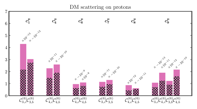
Figure 4: In magenta: the values of nonrelativistic coefficients $c^{p}_{i}$, Eqs. (51)–(56), controlling the scattering of DM on protons, taking only one of the Wilson coefficients nonzero, setting it to ${\cal C}^{(d)}_{a}=1/\Lambda^{2}$, with $\Lambda=1$ TeV. Hatched: the results without QCD resummation, Eqs. (57)–(62).

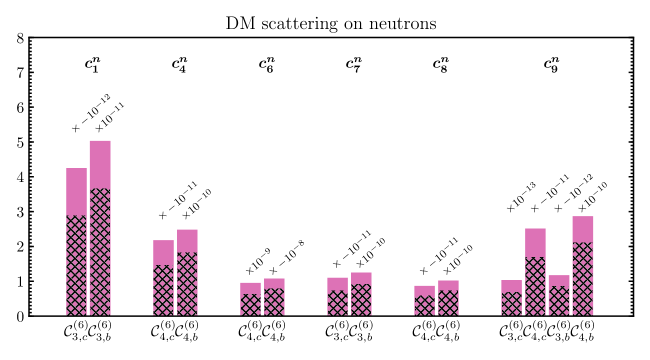
Figure 5: The same as in Fig. 4 but for DM couplings to neutrons, $c^{n}_{i}$.

In Figs. 4 and 5 we show two numerical examples that illustrate the relative importance of the above results. We set $\Lambda=1$ TeV and switch on a single dimension-six Wilson coefficient, ${\cal C}^{(d)}_{3,c}$, ${\cal C}^{(d)}_{4,c}$, ${\cal C}^{(d)}_{3,b}$, or ${\cal C}^{(d)}_{4,b}$ at a time, setting it to ${\cal C}^{(d)}_{a}=1$. Fig. 4 shows the resulting nonrelativistic couplings for SM scattering on protons, $c_{i}^{p}$. The magenta columns are the full results, including QCD resummation. The hatched columns give the results without the QCD resummation from Eqs. (57)–(62). Fig. 5 shows the corresponding results for DM couplings to neutrons, $c_{i}^{n}$.

In these examples we set $\mu_{\rm had}=\mu_{c}=2$ GeV and used the following quark masses at $\mu=m_{Z}$,

$$m_{u}(m_{Z}) =1.4\,\text{MeV}\,, m_{d}(m_{Z}) =3.1\,\text{MeV}\,, m_{s}(m_{Z}) =63\,\text{MeV}\,,$$

$$m_{c}(m_{Z}) =0.78\,\text{GeV}\,, m_{b}(m_{Z}) =3.1\,\text{GeV}\,.$$

These were obtained using the one-loop QCD running to evolve the $\overline{\rm MS}$ quark masses $m_{u,d,s}(2\,\text{GeV})$ and $m_{c(b)}(m_{c(b)})$, taken from Ref. Patrignani et al. (2016), to the common scale $\mu=m_{Z}$. For the nuclear coefficients that depend on the DM mass and/or the momentum transfer, we choose $m_{\chi}=100\,$GeV and a momentum transfer of $q=50\,$MeV.

As seen from Figs. 4 and 5, the resummation of QCD logarithms enhances $c^{p(n)}_{i}$ by approximately $10\%$ to $50\%$ depending on the specific case. The typical enhancement is ${\cal O}(30\%)$. In the numerics we have set the CKM matrix element to unity, thus ignoring all flavor changing transitions. This is a very good approximation for operators with bottom quarks. For charm quarks the effect of flavor off-diagonal CKM matrix elements is more important, yet still subleading. If we including the off-diagonal terms in Eqs. (18)–(19), then the largest correction reaches $16\%$ for $c_{1}^{p}$ induced from ${\cal C}^{(6)}_{3,c}$ ($31\%$ for the result without resummation), as there is an up to $10\%$ cancellation between the ${\cal D}_{3,cu}$ and ${\cal D}_{3,cd}$ contributions with respect to the case of unit CKM matrix. For all other cases the error due to setting the CKM matrix to unity is less than $10\%$.

Finally, we compare the contributions to DM scattering originating from electroweak corrections as opposed to the intrinsic charm and bottom axial charges. For the case of axial-vector–axial-vector interactions (${\cal C}_{4,c}^{(6)}\neq 0$, ${\cal C}_{4,b}^{(6)}\neq 0$) we have

weak: $$c_{4}^{p} \simeq\phantom{+}\frac{1}{\Lambda^{2}}\Big{(}0.02\,{\cal C}_{4,c}^{(6)}-0.26\,{\cal C}_{4,b}^{(6)}\Big{)}\cdot 10^{-3},$$ (63)

intrinsic: $$c_{4}^{p} \simeq-\frac{4}{\Lambda^{2}}\Big{(}\Delta c\,{\cal C}_{4,c}^{(6)}+\Delta b\,{\cal C}_{4,b}^{(6)}\Big{)}\sim-\frac{1}{\Lambda^{2}}\Big{(}2\,{\cal C}_{4,c}^{(6)}+0.2{\cal C}_{4,b}^{(6)}\Big{)}\cdot 10^{-3}.$$ (64)

We see that for the bottom quarks the weak contribution, Eq. (58), is comparable to the contribution from the intrinsic bottom axial charge, while for charm quarks the contribution due to the intrinsic charm axial charge dominates.

For vector–axial-vector interactions (${\cal C}_{3,c}^{(6)}\neq 0$, ${\cal C}_{3,b}^{(6)}\neq 0$) we have

weak: $$c_{1}^{p} \simeq\phantom{+}\frac{1}{\Lambda^{2}}\Big{(}0.4\,{\cal C}_{3,c}^{(6)}-3.0\,{\cal C}_{3,b}^{(6)}\Big{)}\cdot 10^{-6},$$ (65)

intrinsic: $$c_{7}^{p} \simeq-\frac{2}{\Lambda^{2}}\Big{(}\Delta c\,{\cal C}_{3,c}^{(6)}+\Delta b\,{\cal C}_{3,b}^{(6)}\Big{)}\sim-\frac{1}{\Lambda^{2}}\Big{(}{\cal C}_{3,c}^{(6)}+0.1{\cal C}_{3,b}^{(6)}\Big{)}\cdot 10^{-3},$$ (66)

$$c_{9}^{p} \simeq\frac{2}{\Lambda^{2}}\frac{m_{N}}{m_{\chi}}\Big{(}\Delta c\,{\cal C}_{3,c}^{(6)}+\Delta b\,{\cal C}_{3,b}^{(6)}\Big{)}\sim-\frac{1}{\Lambda^{2}}\Big{(}9\,{\cal C}_{3,c}^{(6)}+0.9{\cal C}_{3,b}^{(6)}\Big{)}\cdot 10^{-6},$$ (67)

where in the last equality we set $m_{\chi}=100$ GeV. The effective scattering amplitude is parametrically given by

$${\cal A}\sim Ac_{1}^{p}+v_{T}c_{7}^{p}+\frac{q}{m_{N}}c_{9}^{p},$$ (68)

where $v_{T}\sim 10^{-3}$, $q/m_{N}\lesssim 0.1$, and $A\sim 100$ for heavy nuclei. The loop-induced weak contributions thus dominate the scattering rates of weak scale DM.

VI Connecting to the physics above the weak scale

We now describe how to apply and extend our results for the case in which there is a separation between the mediator scale and the electroweak scale, i.e., if $\Lambda\gg m_{Z}$. In this case, the effective Lagrangian valid above the weak scale is

$${{\mathscr{L}}}_{\chi}=\sum_{a,d}\frac{C_{a}^{(d)}}{\Lambda^{d-4}}Q_{a}^{(d)}\,,$$ (69)

with the operators $Q_{a}^{(d)}$ manifestly invariant under the full SM gauge group. We focus on the dimension-six effective interactions involving DM and quarks currents, analogous to those in Eqs. (2)–(3). For the case of Dirac-fermion DM in a generic $SU(2)_{L}$ representation with generators $\tilde{\tau}^{a}$ and hypercharge $Y_{\chi}$, the basis of dimension-six operators is Bishara et al. (2018)

$$Q_{1,i}^{(6)} =(\bar{\chi}\gamma_{\mu}\tilde{\tau}^{a}\chi)(\bar{Q}_{L}^{i}\gamma^{\mu}\tau^{a}Q_{L}^{i})\,, Q_{5,i}^{(6)} =(\bar{\chi}\gamma_{\mu}\gamma_{5}\tilde{\tau}^{a}\chi)(\bar{Q}_{L}^{i}\gamma^{\mu}\tau^{a}Q_{L}^{i})\,,$$ (70)

$$Q_{2,i}^{(6)} =(\bar{\chi}\gamma_{\mu}\chi)(\bar{Q}_{L}^{i}\gamma^{\mu}Q_{L}^{i})\,, Q_{6,i}^{(6)} =(\bar{\chi}\gamma_{\mu}\gamma_{5}\chi)(\bar{Q}_{L}^{i}\gamma^{\mu}Q_{L}^{i})\,,$$ (71)

$$Q_{3,i}^{(6)} =(\bar{\chi}\gamma_{\mu}\chi)(\bar{u}_{R}^{i}\gamma^{\mu}u_{R}^{i})\,, Q_{7,i}^{(6)} =(\bar{\chi}\gamma_{\mu}\gamma_{5}\chi)(\bar{u}_{R}^{i}\gamma^{\mu}u_{R}^{i})\,,$$ (72)

$$Q_{4,i}^{(6)} =(\bar{\chi}\gamma_{\mu}\chi)(\bar{d}_{R}^{i}\gamma^{\mu}d_{R}^{i})\,, Q_{8,i}^{(6)} =(\bar{\chi}\gamma_{\mu}\gamma_{5}\chi)(\bar{d}_{R}^{i}\gamma^{\mu}d_{R}^{i})\,,$$ (73)

where the index $i=1,2,3$ labels the generation, and $\tau^{a}=\sigma^{a}/2$, with the Pauli matrices $\sigma^{a}$. If $\chi$ is an electroweak singlet, the operators $Q_{1,i}^{(6)}$ and $Q_{5,i}^{(6)}$ do not exist. Below the weak scale the above operators, $Q_{n,i}^{(d)}$, match onto the operators ${\cal Q}_{m,f}^{(d)}$ in Eqs. (2)–(3).

For certain patterns of Wilson coefficients, DM couples only to bottom- and/or charm-quark axial-vector currents. Such possibilities are the main focus of this work. For instance, DM couples (at the mediator scale $\mu\simeq\Lambda\gg m_{Z}$) only to the axial bottom-quark current if the only nonzero Wilson coefficients are $C_{5,3}^{(6)}$, $C_{6,3}^{(6)}$, and $C_{8,3}^{(6)}$, and such that they satisfy the relation

$$Y_{\chi}C_{5,3}^{(6)}=4C_{6,3}^{(6)}=-2C_{8,3}^{(6)}\,.$$ (74)

We first derive the leading electroweak contribution to DM–nucleon scattering rates for this case and then discuss the case in which DM couples only to charm axial currents.

To this end, we fist assume that the initial conditions at $\mu\simeq\Lambda$ satisfy Eq. (74). At scales $\mu_{\rm ew}<\mu<\Lambda$, the operators $Q_{a,i}^{(6)}$ mix at one-loop via the SM Yukawa interactions into the Higgs-current operators Crivellin et al. (2014); D’Eramo and Procura (2015); Bishara et al. (2018)

$$Q_{16}^{(6)} =(\bar{\chi}\gamma^{\mu}\chi)(H^{\dagger}i\overset{\leftrightarrow}{D}_{\mu}H)\,, Q_{18}^{(6)} =(\bar{\chi}\gamma^{\mu}\gamma_{5}\chi)(H^{\dagger}i\overset{\leftrightarrow}{D}_{\mu}H)\,,$$ (75)

and a similar set of operators with the $\tilde{\tau}^{a}\otimes\tau^{a}$ structure (above, $\overset{\leftrightarrow}{D}_{\mu}\,\equiv\,D_{\mu}-\overset{\leftarrow}{D}_{\mu}$). This mixing is generated by “electroweak fish” diagrams, see Fig. 6 (left), and induces at $\mu_{\rm ew}\simeq m_{Z}$

$$C_{16}^{(6)}(m_{Z})\sim\frac{y_{b}^{2}}{16\pi^{2}}C^{(6)}_{a,3}(\Lambda)\log\frac{m_{Z}}{\Lambda}\,,$$ (76)

Here, we only show the parametric dependence and suppress ${\cal O}(1)$ coefficients from the actual value of the anomalous dimensions.

At energies close to the electroweak scale, at which the Higgs obtains its vacuum expectation value, the two operators in Eq. (75) result in couplings of DM currents to the $Z$ boson. Integrating out the $Z$ boson at tree-level induces DM couplings to quarks, see Fig. 6 (right). The Higgs-current operators in Eq. (75) therefore match, at $\mu_{\rm ew}$, onto four-fermion operators of the five-flavor EFT that couple DM to quarks with an interaction strength of parametric size $\sim G_{F}\,C_{16}^{(6)}(m_{Z})\,v^{2}/\Lambda^{2}$. The factor $v^{2}$ originates from the two Higgs fields relaxing to their vacuum expectation values and the factor $G_{F}$ from integrating out the $Z$ boson.

Since the one-loop RG running from $\Lambda$ to $\mu_{\rm ew}$, Eq. (76), followed by tree-level matching at $\mu_{\rm ew}$, induces interactions proportional to $y_{b}^{2}v^{2}$, it is convenient to match such corrections to initial conditions of the dimension-eight operators in Eqs. (24). For the pattern of initial conditions in Eq. (74), we then find that the Wilson coefficient of the dimension-eight operator ${\cal Q}^{(8)}_{4,b}$ at $\mu_{\rm ew}\simeq m_{Z}$ is

$${\cal C}^{(8)}_{4,b}(m_{Z})\sim\frac{g_{s}^{2}}{16\pi^{2}}C_{a,3}^{(6)}(\Lambda)\log\frac{m_{Z}}{\Lambda}\,,$$ (77)

and the Wilson coefficient of the dimension-six operator ${\cal Q}^{(6)}_{4,b}$ is

$${\cal C}^{(6)}_{4,b}(m_{Z})\sim C_{a,3}^{(6)}(\Lambda)\,.$$ (78)

Again, we only show the parametric dependence, including loop factors, but omit ${\mathcal{O}}(1)$ factors, e.g., from the actual values of anomalous dimensions (for details see Ref. Bishara et al. (2018)). In particular, $C_{a,3}^{(6)}(\Lambda)$ denotes a linear combination of the Wilson coefficients with $a=5,6,8$.

The subsequent RG evolution from $\mu_{\rm ew}$ to $\mu_{\rm had}$ proceeds as described in Section V, Eqs. (47)–(50). The only difference is that the initial conditions ${\cal C}^{(8)}_{4,b}(m_{Z})$ are now nonzero. For instance, in the result for the non-relativistic coefficient $c_{4}^{p}$ in Eq. (58), there is an additional contribution from ${\cal C}^{(8)}_{4,b}(m_{Z})\propto\log({m_{Z}}/{\Lambda})$. If one neglects the QCD effects, the two contributions amount to adding up two logarithmically enhanced terms with exactly the same prefactors. The net effect is to replace $\log(m_{q^{\prime}}/m_{Z})$ with $\log(m_{q^{\prime}}/\Lambda)=\log(m_{q^{\prime}}/m_{Z})+\log(m_{Z}/\Lambda)$ in Eqs. (57)–(62). This is equivalent to simply calculating the electroweak fish diagram, with $u,d,s$ fermions attached to the $Z$ line, and keeping only the $\log(m_{b}/\Lambda)$-enhanced part.

Figure 6: Left: “electroweak fish” diagram that induces the mixing of $Q_{a,i}^{(6)}$ operators into the Higgs operators, $Q_{16}^{(6)}$. Right: tree-level diagram that generates the dimension-eight operators from the Higgs operators through matching at the weak scale.

An analogous analysis applies if the only nonzero Wilson coefficients satisfy $Y_{\chi}C_{5,2}^{(6)}=-4C_{6,2}^{(6)}=2C_{7,2}^{(6)}$, so that just the $(\bar{\chi}\gamma_{\mu}\gamma_{5}\chi)(\bar{c}\gamma^{\mu}\gamma_{5}c)$ operator is generated (setting the CKM matrix to unity for simplicity). Similarly, if the only nonzero Wilson coefficients satisfy $Y_{\chi}C_{1,3}^{(6)}=4C_{2,3}^{(6)}=-2C_{4,3}^{(6)}\neq 0$ or $Y_{\chi}C_{1,2}^{(6)}=-4C_{2,2}^{(6)}=2C_{3,2}^{(6)}\neq 0$ this means that just the $(\bar{\chi}\gamma_{\mu}\chi)(\bar{b}\gamma^{\mu}\gamma_{5}b)$ or $(\bar{\chi}\gamma_{\mu}\chi)(\bar{c}\gamma^{\mu}\gamma_{5}c)$ operators are generated. Such relations do not necessarily imply fine-tuning, as they can originate from the quantum number assignments for the mediators, DM, and quark fields in the UV theory. They do require the DM hypercharge $Y_{\chi}$ to be nonzero. This conclusion changes, if at $\mu\simeq\Lambda$ we also include dimension-eight operators of the form $(\bar{\chi}\gamma_{\mu}\chi)(\bar{Q}_{L}H\gamma^{\mu}HQ_{L})$ alongside the dimension-six $(\bar{\chi}\gamma_{\mu}\chi)(\bar{b}_{R}\gamma^{\mu}b_{R})$ operators. In this case, it is possible to induce only the $(\bar{\chi}\gamma_{\mu}\chi)(\bar{b}\gamma^{\mu}\gamma_{5}b)$ or $(\bar{\chi}\gamma_{\mu}\chi)(\bar{c}\gamma^{\mu}\gamma_{5}c)$ operators even for DM with zero hypercharge (and thus without a renormalizable interaction to the $Z$ boson). This, however, requires fine-tuning of dimension-six and dimension-eight contributions.

Note that the relation in Eq. (74) also requires DM to be part of an electroweak multiplet. For singlet DM there is no operator $Q_{5,i}^{(6)}$ and so $C_{5,i}^{(6)}$ is trivially zero. Therefore, for singlet DM a coupling to an axial-vector bottom-quark current is always accompanied by couplings to top quarks. In this case our results get corrected by terms of order $y_{t}^{2}\log(\mu_{\rm ew}/\Lambda)$ from the RG evolution above the electroweak scale due to top-Yukawa interactions Bishara et al. (2018).

Another phenomenologically interesting case is the one of DM coupling only to leptons at $\mu_{\rm ew}$, i.e., through operators in Eqs. (2)–(3) with $f=e,\mu,\tau$. We can readily adapt our results to this case by replacing in Eqs. (13)–(17) the bottom- and charm-quarks with leptons. The new operators are either color-singlets or conserved QCD currents so that their anomalous dimensions vanish. The hadronic functions $c_{i}^{p(n)}$, controlling DM scattering on nuclei, are then given by Eqs. (57)–(62) after substituting $q^{\prime}\to{\ell=\tau,\mu}$, and dividing by the number of colors, $N_{c}=3$, implicit in these equations. For $\ell=\mu,\tau$ there are no other numerically competing contributions from other dimension-eight operators apart from the ones we discussed here. However, for the electron case, $\ell=e$, we expect dimension-eight operators with derivatives, which we have not considered here, to contribute to the scattering on nuclei at approximately the same order.

VII Majorana and scalar dark matter

So far we focused on DM that is a Dirac fermion. However, the RG results discussed in this work do not depend on the precise form of the DM current. We can, therefore, generalize our results to the case of Majorana and scalar DM.

VII.1 Majorana dark matter

Our results apply for Majorana DM with only small modifications. It is sufficient to drop from the operator basis the operators ${\cal Q}_{1,f}^{(6)}$ and ${\cal Q}_{3,f}^{(6)}$ in Eqs. (2)–(3) and likewise the operators ${\cal Q}_{1,q}^{(8)}$ and ${\cal Q}_{3,q}^{(8)}$ in Eqs. (23)–(24). The Lagrangian terms proportional to the remaining operators, ${\cal Q}_{2,f}^{(6)}$, ${\cal Q}_{4,f}^{(6)}$, ${\cal Q}_{2,f}^{(8)}$, and ${\cal Q}_{4,f}^{(8)}$ should be multiplied by a factor of $1/2$ to account for the additional Wick contractions (see, for instance, Ref. Bishara et al. (2017c)). With these modifications, the coefficients of the nuclear effective theory are still given by Eqs. (51)–(56).

VII.2 Scalar dark matter

The relevant set of operators for scalar DM is

$${\cal Q}_{1,f}^{(6)} =\big{(}\varphi^{*}i\overset{\!\!\leftrightarrow}{\partial_{\mu}}\varphi\big{)}(\bar{f}\gamma^{\mu}f)\,, {\cal Q}_{2,f}^{(6)} =\big{(}\varphi^{*}i\overset{\!\!\leftrightarrow}{\partial_{\mu}}\varphi\big{)}(\bar{f}\gamma^{\mu}\gamma_{5}f)\,,$$ (79)

where $\varphi^{*}\overset{\!\!\leftrightarrow}{\partial_{\mu}}\varphi\equiv\varphi^{*}\partial_{\mu}\varphi-(\partial_{\mu}\varphi^{*})\varphi$. These operators are part of the dimension-six effective Lagrangian for scalar DM, cf., Ref. Bishara et al. (2017a),

$${{\mathscr{L}}}_{\varphi}=\sum_{a}\frac{{\cal C}_{a}^{(6)}}{\Lambda^{2}}{\cal Q}_{a}^{(6)}\,,$$ (80)

with ${\cal C}_{a}^{(6)}$ the dimensionless Wilson coefficients. Note that we adopt the same notation for operators and Wilson coefficients in the case of scalar DM as we did for fermionic DM. No confusion should arise as this abuse of notation is restricted to this subsection.

Apart from having a different DM current, nothing changes in our calculations. Therefore, after defining the dimension-eight effective Lagrangian in the three-flavor theory as

$${{\mathscr{L}}}_{\varphi}^{(8)}=-\frac{\sqrt{2}G_{F}}{\Lambda^{2}}\sum_{q=u,d,s}\Big{(}{\cal C}_{1,q}^{(8)}\frac{m_{q}^{2}}{g_{s}^{2}}\big{(}\varphi^{*}i\overset{\!\!\leftrightarrow}{\partial_{\mu}}\varphi\big{)}(\bar{q}\gamma^{\mu}q)+{\cal C}_{2,f}^{(8)}\frac{m_{q}^{2}}{g_{s}^{2}}\big{(}\varphi^{*}i\overset{\!\!\leftrightarrow}{\partial_{\mu}}\varphi\big{)}(\bar{q}\gamma^{\mu}\gamma_{5}q)\Big{)}\,,$$ (81)

the additional contributions to the nuclear coefficients are given, for complex scalar DM, by (cf. Ref. Bishara et al. (2017c))

$$c_{1}^{N} =-\frac{1}{2\pi\alpha_{s}}\frac{\sqrt{2}G_{F}}{\Lambda^{2}}m_{\varphi}\sum_{q=u,d,s}m_{q}^{2}\,{\cal C}_{1q}^{(8)}\,F_{1}^{q/N}\,,$$ (82)

$$c_{7}^{N} =\phantom{+}\leavevmode\nobreak\ \,\frac{1}{\pi\alpha_{s}}\frac{\sqrt{2}G_{F}}{\Lambda^{2}}m_{\varphi}\sum_{q=u,d,s}m_{q}^{2}\,{\cal C}_{2q}^{(8)}\,F_{A}^{q/N}\,.$$ (83)

For real scalar DM, the operators in Eq. (79) vanish. For completeness, we display also the dimension-eight contributions to the nuclear coefficients, expanded to leading order in the strong coupling constant,

$$c_{1}^{N}\simeq \phantom{+}\leavevmode\nobreak\ \,\leavevmode\nobreak\ \frac{6m_{\varphi}}{\pi^{2}}\frac{\sqrt{2}G_{F}}{\Lambda^{2}}\sum_{q^{\prime}=c,b}m_{q^{\prime}}^{2}\,\log\frac{\mu_{q^{\prime}}}{m_{Z}}\,{\cal C}_{2,q^{\prime}}^{(6)}(m_{Z})\,\sum_{q=u,d,s}{\cal D}_{3,q^{\prime}q}F_{1}^{q/N}+{\mathcal{O}}(\alpha_{s})\,,$$ (84)

$$c_{7}^{N}\simeq -\frac{12m_{\varphi}}{\pi^{2}}\frac{\sqrt{2}G_{F}}{\Lambda^{2}}\sum_{q^{\prime}=c,b}m_{q^{\prime}}^{2}\,\log\frac{\mu_{q^{\prime}}}{m_{Z}}\,{\cal C}_{2,q^{\prime}}^{(6)}(m_{Z})\,\sum_{q=u,d,s}{\cal D}_{2,qq^{\prime}}F_{A}^{q/N}+{\mathcal{O}}(\alpha_{s})\,.$$ (85)

VIII Conclusions

If DM couples only to bottom- or charm-quark axial-vector currents, the dominant contribution to DM scattering on nuclei is either due to one-loop electroweak corrections or due to the intrinsic bottom and charm axial charges of the nucleons. Below the weak scale the electroweak contributions are captured by double insertions of both the DM effective Lagrangian and the SM weak effective Lagrangian. These convert the heavy-quark currents to the currents with $u,d$, and $s$ quarks that have nonzero nuclear matrix elements. In this paper we calculated the nonrelativistic couplings of DM to neutrons and protons that result from such electroweak corrections, including the resummation of the leading-logarithmic QCD corrections. The latter are numerically important, as they lead to ${\mathcal{O}}(1)$ changes in the scattering rates on nuclei. Our results can be readily included in the general framework of EFT for DM direct detection, and will be implemented in a future version of the public code DirectDM Bishara et al. (2017c).

Acknowledgements. We thank Francesco D’Eramo for useful discussions, and especially Fady Bishara for checking several equations. JZ acknowledges support in part by the DOE grant DE-SC0011784. The research of BG was supported in part by the DOE Grant No. DE-SC0009919.

Appendix A Unphysical operators

We extract the anomalous dimensions by renormalizing off-shell Green’s functions in $d=4-2\epsilon$ dimensions. In some intermediate stages of the computation it is thus necessary to introduce some unphysical operators.

A.1 Evanescent operators

The one-loop mixing among the “physical” operators is not affected by the definition of evanescent operators, i.e., operators that are required to project one-loop Green’s functions in $d=4-2\epsilon$ dimensions but vanish in $d=4$. Indeed, our one-loop results could also have been obtained by performing the Dirac algebra in $d=4$ instead off in non-integer dimensions. Since i) this no longer possible at next-to-leading order computations and ii) we use dimensional regularization to extract the poles of loop integrals, we find it convenient to also perform the Dirac algebra in non-integer dimensions. To project the $d=4-2\epsilon$ amplitudes we thus need to also include some evanescent operators in the basis. For completeness and future reference, we list below the ones entering the one-loop computations.

$$\begin{split}{\cal E}_{1}^{qq^{\prime}}&=(\bar{q}\gamma^{\mu}\gamma^{\nu}\gamma^{\rho}q)\,(\bar{q}^{\prime}\gamma_{\mu}\gamma_{\nu}\gamma_{\rho}q^{\prime})-10{\cal O}_{1}^{qq^{\prime}}-6{\cal O}_{2}^{qq^{\prime}}\,,\\[5.0pt] {\cal E}_{2}^{qq^{\prime}}&=(\bar{q}\gamma^{\mu}\gamma^{\nu}\gamma^{\rho}\gamma_{5}q)\,(\bar{q}^{\prime}\gamma_{\mu}\gamma_{\nu}\gamma_{\rho}\gamma_{5}q^{\prime})-6{\cal O}_{1}^{qq^{\prime}}-10{\cal O}_{2}^{qq^{\prime}}\,,\\[5.0pt] {\cal E}_{3}^{qq^{\prime}}&=(\bar{q}\gamma^{\mu}\gamma^{\nu}\gamma^{\rho}\gamma_{5}q)\,(\bar{q}^{\prime}\gamma_{\mu}\gamma_{\nu}\gamma_{\rho}q^{\prime})-10{\cal O}_{3}^{qq^{\prime}}-6{\cal O}_{3}^{q^{\prime}q}\,,\\[5.0pt] {\cal E}_{4}^{qq^{\prime}}&=(\bar{q}\gamma^{\mu}\gamma^{\nu}\gamma^{\rho}\,T^{a}q)\,(\bar{q}^{\prime}\gamma_{\mu}\gamma_{\nu}\gamma_{\rho}\,T^{a}q^{\prime})-10{\cal O}_{4}^{qq^{\prime}}-6{\cal O}_{5}^{q^{\prime}q}\,,\\[5.0pt] {\cal E}_{5}^{qq^{\prime}}&=(\bar{q}\gamma^{\mu}\gamma^{\nu}\gamma^{\rho}\gamma_{5}\,T^{a}q)\,(\bar{q}^{\prime}\gamma_{\mu}\gamma_{\nu}\gamma_{\rho}\gamma_{5}\,T^{a}q^{\prime})-6{\cal O}_{4}^{qq^{\prime}}-10{\cal O}_{5}^{q^{\prime}q}\,,\\[5.0pt] {\cal E}_{6}^{qq^{\prime}}&=(\bar{q}\gamma^{\mu}\gamma^{\nu}\gamma^{\rho}\gamma_{5}\,T^{a}q)\,(\bar{q}^{\prime}\gamma_{\mu}\gamma_{\nu}\gamma_{\rho}\,T^{a}q^{\prime})-10{\cal O}_{6}^{qq^{\prime}}-6{\cal O}_{6}^{q^{\prime}q}\,,\end{split}$$ (86)

and

$$\begin{split}{\cal E}_{1}^{q}&=(\bar{q}\gamma^{\mu}\gamma^{\nu}\gamma^{\rho}q)\,(\bar{q}\gamma_{\mu}\gamma_{\nu}\gamma_{\rho}q)-10{\cal O}_{1}^{q}-6{\cal O}_{2}^{q}\,,\\[5.0pt] {\cal E}_{2}^{q}&=(\bar{q}\gamma^{\mu}\gamma^{\nu}\gamma^{\rho}\gamma_{5}q)\,(\bar{q}\gamma_{\mu}\gamma_{\nu}\gamma_{\rho}\gamma_{5}q)-6{\cal O}_{1}^{q}-10{\cal O}_{2}^{q}\,,\\[5.0pt] {\cal E}_{3}^{q}&=(\bar{q}\gamma^{\mu}\gamma^{\nu}\gamma^{\rho}\gamma_{5}q)\,(\bar{q}\gamma_{\mu}\gamma_{\nu}\gamma_{\rho}q)-16{\cal O}_{3}^{q}\,,\\[5.0pt] {\cal E}_{4}^{q}&=(\bar{q}\gamma^{\mu}\gamma^{\nu}\gamma^{\rho}\,T^{a}q)\,(\bar{q}\gamma_{\mu}\gamma_{\nu}\gamma_{\rho}\,T^{a}q)-3\bigg{(}1-\frac{1}{N_{c}}\bigg{)}\big{(}{\cal O}_{1}^{q}+{\cal O}_{2}^{q}\big{)}-4{\cal O}_{4}^{q}\,,\\[5.0pt] {\cal E}_{5}^{q}&=(\bar{q}\gamma^{\mu}\gamma^{\nu}\gamma^{\rho}\gamma_{5}\,T^{a}q)\,(\bar{q}\gamma_{\mu}\gamma_{\nu}\gamma_{\rho}\gamma_{5}\,T^{a}q)-5\bigg{(}1-\frac{1}{N_{c}}\bigg{)}\big{(}{\cal O}_{1}^{q}+{\cal O}_{2}^{q}\big{)}+4{\cal O}_{4}^{q}\,,\\[5.0pt] {\cal E}_{6}^{q}&=(\bar{q}\gamma^{\mu}\gamma^{\nu}\gamma^{\rho}\gamma_{5}\,T^{a}q)\,(\bar{q}\gamma_{\mu}\gamma_{\nu}\gamma_{\rho}\,T^{a}q)-8\bigg{(}1-\frac{1}{N_{c}}\bigg{)}{\cal O}_{3}^{q}\,,\\[5.0pt] {\cal E}_{7}^{q}&=(\bar{q}\gamma^{\mu}\gamma_{5}\,T^{a}q)\,(\bar{q}\gamma_{\mu}\gamma_{5}\,T^{a}q)-\frac{1}{2}\bigg{(}1-\frac{1}{N_{c}}\bigg{)}\big{(}{\cal O}_{1}^{q}+{\cal O}_{2}^{q}\big{)}+{\cal O}_{4}^{q}\,,\\[5.0pt] {\cal E}_{8}^{q}&=(\bar{q}\gamma^{\mu}\gamma_{5}\,T^{a}q)\,(\bar{q}\gamma_{\mu}\,T^{a}q)-\frac{1}{2}\bigg{(}1-\frac{1}{N_{c}}\bigg{)}{\cal O}_{3}^{q}\,.\end{split}$$ (87)

Here, $N_{c}=3$ denotes the number of colors. The operators ${\cal E}^{q}_{7}$ and ${\cal E}^{q}_{8}$ are Fierz-evanenscent operators, i.e., they vanish due to Fierz identities and not due to special $d=4$ relations of the Dirac algebra.

A.2 E.o.m.-vanishing operators

In our conventions the equation of motion (e.o.m.) for the gluon field reads

$$\begin{split}D^{\nu}G^{a}_{\nu\mu}\equiv(\partial^{\nu}\delta^{ab}-g_{s}f^{abc}G^{\nu,c})G^{b}_{\nu\mu}=-g_{s}\sum_{q}\bar{q}T^{a}\gamma_{\mu}q\,,\end{split}$$ (88)

up to gauge-fixing and ghost terms. The sum is over all active quark fields. Hence the following operators vanish via the e.o.m.

$$\begin{split}{\cal N}_{1,\text{e.o.m.}}^{q}&=\frac{1}{g_{s}}(\bar{q}\gamma^{\mu}\,T^{a}q)D^{\nu}G^{a}_{\nu\mu}+{\cal O}_{4,q}^{(6)}+\sum_{q^{\prime}\neq q}{\cal O}_{4,qq^{\prime}}^{(6)}\,,\\ {\cal N}_{2,\text{e.o.m.}}^{q}&=\frac{1}{g_{s}}(\bar{q}\gamma^{\mu}\gamma_{5}\,T^{a}q)D^{\nu}G^{a}_{\nu\mu}+\frac{1}{2}\bigg{(}1-\frac{1}{N_{c}}\bigg{)}{\cal O}_{3}^{q}+\sum_{q^{\prime}\neq q}{\cal O}_{6,qq^{\prime}}^{(6)}\,.\end{split}$$ (89)

The four-fermion pieces of these e.o.m.-vanishing operators contribute to the same amplitudes as the physical four-fermion operators. Therefore, the mixing of physical operators into the e.o.m.-vanishing operators (computed from QCD penguin diagrams, Fig. 3) affects the anomalous dimensions of four-fermion operators.

References

• Bagnasco et al. (1994) J. Bagnasco, M. Dine, and S. D. Thomas, Phys. Lett. B320, 99 (1994), eprint hep-ph/9310290.
• Kurylov and Kamionkowski (2004) A. Kurylov and M. Kamionkowski, Phys. Rev. D69, 063503 (2004), eprint hep-ph/0307185.
• Kopp et al. (2010) J. Kopp, T. Schwetz, and J. Zupan, JCAP 1002, 014 (2010), eprint 0912.4264.
• Goodman et al. (2011) J. Goodman, M. Ibe, A. Rajaraman, W. Shepherd, T. M. P. Tait, and H.-B. Yu, Nucl. Phys. B844, 55 (2011), eprint 1009.0008.
• Goodman et al. (2010) J. Goodman, M. Ibe, A. Rajaraman, W. Shepherd, T. M. Tait, et al., Phys.Rev. D82, 116010 (2010), eprint 1008.1783.
• Bai et al. (2010) Y. Bai, P. J. Fox, and R. Harnik, JHEP 12, 048 (2010), eprint 1005.3797.
• Hill and Solon (2012) R. J. Hill and M. P. Solon, Phys.Lett. B707, 539 (2012), eprint 1111.0016.
• Cirelli et al. (2013) M. Cirelli, E. Del Nobile, and P. Panci, JCAP 1310, 019 (2013), eprint 1307.5955.
• Hill and Solon (2015) R. J. Hill and M. P. Solon, Phys.Rev. D91, 043505 (2015), eprint 1409.8290.
• Crivellin et al. (2014) A. Crivellin, F. D’Eramo, and M. Procura, Phys. Rev. Lett. 112, 191304 (2014), eprint 1402.1173.
• D’Eramo and Procura (2015) F. D’Eramo and M. Procura, JHEP 04, 054 (2015), eprint 1411.3342.
• Hill and Solon (2014) R. J. Hill and M. P. Solon, Phys. Rev. Lett. 112, 211602 (2014), eprint 1309.4092.
• Hoferichter et al. (2015) M. Hoferichter, P. Klos, and A. Schwenk, Phys. Lett. B746, 410 (2015), eprint 1503.04811.
• Bishara et al. (2017a) F. Bishara, J. Brod, B. Grinstein, and J. Zupan, JCAP 1702, 009 (2017a), eprint 1611.00368.
• D’Eramo et al. (2016) F. D’Eramo, B. J. Kavanagh, and P. Panci, JHEP 08, 111 (2016), eprint 1605.04917.
• Bishara et al. (2017b) F. Bishara, J. Brod, B. Grinstein, and J. Zupan, JHEP 11, 059 (2017b), eprint 1707.06998.
• D’Eramo et al. (2017) F. D’Eramo, B. J. Kavanagh, and P. Panci, Phys. Lett. B771, 339 (2017), eprint 1702.00016.
• Bishara et al. (2017c) F. Bishara, J. Brod, B. Grinstein, and J. Zupan (2017c), eprint 1708.02678.
• Brod et al. (2017) J. Brod, A. Gootjes-Dreesbach, M. Tammaro, and J. Zupan (2017), eprint 1710.10218.
• Fitzpatrick et al. (2013) A. L. Fitzpatrick, W. Haxton, E. Katz, N. Lubbers, and Y. Xu, JCAP 1302, 004 (2013), eprint 1203.3542.
• Fitzpatrick et al. (2012) A. L. Fitzpatrick, W. Haxton, E. Katz, N. Lubbers, and Y. Xu (2012), eprint 1211.2818.
• Anand et al. (2014) N. Anand, A. L. Fitzpatrick, and W. C. Haxton, Phys. Rev. C89, 065501 (2014), eprint 1308.6288.
• Hoferichter et al. (2016) M. Hoferichter, P. Klos, J. Menéndez, and A. Schwenk, Phys. Rev. D94, 063505 (2016), eprint 1605.08043.
• Bali et al. (2012) G. S. Bali et al. (QCDSF), Phys. Rev. Lett. 108, 222001 (2012), eprint 1112.3354.
• Engelhardt (2012) M. Engelhardt, Phys. Rev. D86, 114510 (2012), eprint 1210.0025.
• Bhattacharya et al. (2014) T. Bhattacharya, R. Gupta, and B. Yoon, PoS LATTICE2014, 141 (2014), eprint 1503.05975.
• Alexandrou et al. (2017) C. Alexandrou, M. Constantinou, K. Hadjiyiannakou, K. Jansen, C. Kallidonis, G. Koutsou, and A. Vaquero Aviles-Casco (2017), eprint 1705.03399.
• Polyakov et al. (1999) M. V. Polyakov, A. Schafer, and O. V. Teryaev, Phys. Rev. D60, 051502 (1999), eprint hep-ph/9812393.
• Witten (1977) E. Witten, Nucl. Phys. B122, 109 (1977).
• Gilman and Wise (1983) F. J. Gilman and M. B. Wise, Phys. Rev. D27, 1128 (1983).
• Flynn (1990) J. M. Flynn, Mod. Phys. Lett. A5, 877 (1990).
• Datta et al. (1990) A. Datta, J. Frohlich, and E. A. Paschos, Z. Phys. C46, 63 (1990).
• Herrlich and Nierste (1995) S. Herrlich and U. Nierste, Nucl. Phys. B455, 39 (1995), eprint hep-ph/9412375.
• Herrlich and Nierste (1996) S. Herrlich and U. Nierste, Nucl. Phys. B476, 27 (1996), eprint hep-ph/9604330.
• Brod and Zupan (2014) J. Brod and J. Zupan, JHEP 01, 051 (2014), eprint 1308.5663.
• Brod (2015) J. Brod, Phys. Lett. B743, 56 (2015), eprint 1412.3173.
• Patrignani et al. (2016) C. Patrignani et al. (Particle Data Group), Chin. Phys. C40, 100001 (2016).
• Bishara et al. (2018) F. Bishara, J. Brod, B. Grinstein, and J. Zupan, to appear (2018).