A Simple and Efficient Estimation Method for Models with Nonignorable Missing Data

Abstract

This paper proposes a simple and efficient estimation procedure for the model with non-ignorable missing data studied by Morikawa and Kim (2016). Their semiparametrically efficient estimator requires explicit nonparametric estimation and so suffers from the curse of dimensionality and requires a bandwidth selection. We propose an estimation method based on the Generalized Method of Moments (hereafter GMM). Our method is consistent and asymptotically normal regardless of the number of moments chosen. Furthermore, if the number of moments increases appropriately our estimator can achieve the semiparametric efficiency bound derived in Morikawa and Kim (2016), but under weaker regularity conditions. Moreover, our proposed estimator and its consistent covariance matrix are easily computed with the widely available GMM package. We propose two data-based methods for selection of the number of moments. A small scale simulation study reveals that the proposed estimation indeed out-performs the existing alternatives in finite samples.

Keywords: Nonignorable nonresponse; Generalized method of moments; Semiparametric efficiency.

1 Introduction

Missing data is common in many fields of applications. One way to deal with the missing data problem is to delete observations containing missing data. In doing so we may produce biased estimates and erroneous conclusions, depending on the data missing mechanism. If data are missing completely at random, standard estimation and inference procedures are still consistent when the missing data observations are ignored, see Heitjan and Basu (1996), Little (1988) among others. If data are missing at random (MAR) in the sense that the propensity of missingness depends only on the observed covariates, consistent estimation can still be obtained through covariate balancing, see Rubin (1976a, b), Little and Rubin (1989), Robins and Rotnitzky (1995), Robins et al. (1995), Bang and Robins (2005), Qin and Zhang (2007), Chen et al. (2008), Tan (2010), Rotnitzky et al. (2012), Little and Rubin (2014) among others. In many applications, data are missing not at random (MNAR). For example, the income question in sample surveys is often not answered by people at the top end of the distribution, that is, their response frequency depends on an outcome variable that is often the key focus. An investigator is examining the effect of sleep on pain by calling subjects daily to ask them about last night’s sleep and their pain today. Patients who are experiencing severe pain are more likely to not come to the phone leaving the data missing for that particular day; again this would violate the MAR assumption. From political science, roll-call votes, which measure legislatures ideological positions, are subject to non-ignorable nonresponse because, unsurprisingly, politicians behave strategically. In the MNAR case, the parameter of interest may not even be identified (e.g., Robins et al. (1997)), let alone be consistently estimated. To be more specific, let $T\in\{0,1\}$ denote the binary random variable indicating the missing status of the outcome variable $Y$: $Y$ is observed if $T$ takes the value one and $Y$ is not observed if $T$ takes the value zero. Let $\boldsymbol{X}$ denote a vector of explanatory variables, let $\pi(\boldsymbol{x},y)=\mathbb{P}(T=1|\boldsymbol{X}=\boldsymbol{x},Y=y)$ denote the propensity score function and let $f_{Y|\boldsymbol{X}}(y|\boldsymbol{x})$ denote the conditional density function of $Y$ given $\boldsymbol{X}$. Robins et al. (1997) shows that if both the propensity score function and the conditional density function are completely unknown, the joint  distribution of $(T,Y)$ given $\boldsymbol{X}$ is not point identifiable. In this case, a necessary identification condition is the parameterization of either the propensity score function or the conditional density function. Molenberghs and Kenward (2007) proposes the parameterization of both the propensity score function and the conditional density function as an identification strategy, while Sverchkov (2008) and Riddles et al. (2016) parameterize the propensity score function and only a component of the conditional density function: $f_{Y|\boldsymbol{X},T}(y|\boldsymbol{x},T=1)$.

If the joint distribution is not the parameter of interest, the identification strategy above can be modified. For example, if the parameter of interest is the conditional density of $Y$ given $\boldsymbol{X}$ (i.e., $f_{Y|\boldsymbol{X}}(y|\boldsymbol{x})$), parameterization of the propensity score function is not needed. However, parameterization of $f_{Y|\boldsymbol{X}}(y|\boldsymbol{x})$ in this case is not sufficient for identification due to missing data. Tang et al. (2003) suggests parameterization of the marginal density $f_{\boldsymbol{X}}(\boldsymbol{x})$ as well, while Zhao and Shao (2015) imposes an exclusion retriction. In both studies, $f_{Y|\boldsymbol{X}}(y|\boldsymbol{x})$ is identified and consistently estimated.

We consider estimation of the parameter $\theta_{0}=\mathbb{E}[U(\boldsymbol{X},Y)]$, where $U(\cdot)$ is any known function. We suppose that the propensity score $\pi$ is parameterized but do not restrict the conditional density function of the outcome variable. In earlier work in this framework, either the coefficients in the propensity score function are known or consistently estimated from an external sample (Kim and Yu (2011)) or an exclusion restriction is imposed (Wang et al. (2014) and Shao and Wang (2016)). Morikawa and Kim (2016) study the efficient estimation of $\theta_{0}$. They derive the efficient score function (and hence the semiparametric efficiency bound) for $\theta_{0}$ in this model. They propose to estimate the efficient score function by estimating $f_{Y|\boldsymbol{X},T}(y|,\boldsymbol{x},1)$ by a working parametric model (MK1) or by kernel nonparametric estimation (MK2). Their approach MK1 is not efficient unless the working parametric model is correct, although it is consistent. Their method MK2 suffers from the curse of dimensionality (their smoothness conditions depend on the dimensionality of the covariates through their conditions C14) and the bandwidth selection problem (about which they give no guidance).

We study the same estimation problem as in Morikawa and Kim (2016) but propose a simpler yet equally efficient estimation procedure. Our proposed method does not require explicit nonparametric estimation and hence does not suffer from the curse of dimensionality. The proposed estimator is motivated by the key insight that the model parameter satisfies a parametric conditional moment restriction, of which the semiparametric efficiency bound is identical to the bound derived in Morikawa and Kim (2016). The conditional moment restriction is then turned into an expanding set of unconditional moment restrictions and the parameter of interest is estimated by applying the widely available and easy to compute GMM estimation (see Hansen (1982)). Under some sufficient conditions, we establish that the proposed estimator is consistent and asymptotically normally distributed even if the set of unconditional moment restrictions does not expand, thereby freeing us from the curse of dimensionality and the bandwidth selection problem; when the set does expand, the proposed estimator attains the semiparametric efficiency bound. This is in contrast with the MK2 method of Morikawa and Kim (2016), which is inconsistent if the bandwidth does not go to zero at a certain rate.

The paper is organized as follows. Section 2 describes the estimation, Section 3 derives the large sample properties of the estimator, Section 4 provides a consistent asymptotic variance estimator, Section 5 suggests two data driven approaches to determine the number of unconditional moment restrictions, Section 6 reports on a small scale simulation study, followed by some concluding remarks in Section 7. All technical proofs are relegated to the Appendix.

2 Basic Framework and Estimation

We begin by setting up the basic framework. Denote $\boldsymbol{Z}=(\boldsymbol{X}^{\top},Y)^{\top}$. The following assumption shall be maintained throughout the paper:

Assumption 2.1. (i) Parameterization of data missing mechanism: $\mathbb{P}(T=1|Y,\boldsymbol{X})=\pi(Y,\boldsymbol{X};\gamma_{0})=\pi(\boldsymbol{Z};\gamma_{0})$ holds for some known function $\pi(.;.)$, where $\gamma_{0}\in\mathbb{R}^{p}$ for some known $p\in\mathbb{N}$ is the true (unknown) value; (ii) exclusion restriction: there exists some nonresponse instrument variables $\boldsymbol{X}_{1}$ in $\boldsymbol{X}=(\boldsymbol{X}_{1}^{\top},\boldsymbol{X}_{2}^{\top})^{\top}$ so that $\boldsymbol{X}_{2}$ is independent of $T$ given both $\boldsymbol{X}_{1}$ and $Y$; and (iii) the parameter of interest is $\theta_{0}=\mathbb{E}[U(\boldsymbol{Z})]$ for some known function $U(\cdot)$.

Under Assumption 2.1 and by applying the law of iterated expectations, we obtain the following conditional moment restrictions:

$$\mathbb{E}\left[1-\frac{T}{\pi(\boldsymbol{Z};\gamma_{0})}\bigg{|}\boldsymbol{X}\right]=0,$$ (1)

$$\mathbb{E}\left[\theta_{0}-\frac{T}{\pi(\boldsymbol{Z};\gamma_{0})}U(\boldsymbol{Z})\right]=0,$$ (2)

which will form the basis for the proposed estimation. We notice that the parameters of interest in (1)-(2) are finite dimensional (and there is no explicit infinite dimensional nuisance parameter) and can be easily estimated with GMM estimation. We also notice that it is a special case of the model studied in Ai and Chen (2012). By applying their result (Remark 2.1, pp. 446), we obtain the semiparametric efficiency bound for model (1)-(2), which is identical to the bound derived in Morikawa and Kim (2016), thereby suggesting a simple and efficient estimation.

The (nuisance) parameter $\gamma_{0}$ is identified by (1) and the parameter of interest $\theta_{0}$ is identified by (2). The following condition shall also be maintained throughout the paper:

Assumption 2.2. The parameter space $\Gamma$ is a compact subset of $\mathbb{R}^{p}$. The true value $\gamma_{0}$ lies in the interior of $\Gamma$ and is the only solution to (1). The parameter space $\Theta$ is a compact subset of $\mathbb{R}$ and the true value $\theta_{0}$ lies in the interior of $\Theta$.

To estimate model (1)-(2), we first turn it into a set of unconditional moment restrictions. We work with a set of known basis functions: for each integer $\ K\in\mathbb{N}\ \text{with}\ K\geq p\$, let

$$u_{K}(\boldsymbol{X})=(u_{1K}(\boldsymbol{X}),\ldots,u_{KK}(\boldsymbol{X}))^{\top}.\$$

Discussion on the choice of $u_{K}(\boldsymbol{X})$ and its properties can be found in Section 8.2 in Appendix. Model (1)-(2) implies the unconditional moment restrictions:

$$\mathbb{E}\left[\left(1-\frac{T}{\pi(\boldsymbol{Z};\gamma_{0})}\right)u_{K}(\boldsymbol{X})\right]=0,$$ (3)

$$\mathbb{E}\left[\theta_{0}-\frac{T}{\pi(\boldsymbol{Z};\gamma_{0})}U(\boldsymbol{Z})\right]=0.$$ (4)

To avoid redundant moment restrictions, we require $\mathbb{E}\left[u_{K}(\boldsymbol{X})u_{K}(\boldsymbol{X})^{\top}\right]$ to be nonsingular for every $K$. The following somewhat stronger identification condition shall be maintained throughout the paper:

Assumption 2.2’. The parameter space $\Gamma$ is a compact subset of $\mathbb{R}^{p}$. The true value $\gamma_{0}$ lies in the interior of $\Gamma$ and is the only solution to (3). The parameter space $\Theta$ is a compact subset of $\mathbb{R}$ and the true value $\theta_{0}$ lies in the interior of $\Theta$.

We can estimate the parameter of interest by the GMM method. Let $\{T_{i},\boldsymbol{Z}_{i}\}_{i=1}^{N}$ denote an $i.i.d\text{.}$ sample drawn from the joint distribution of $(T,\boldsymbol{Z})$. Denote

$$\boldsymbol{G}_{K}(\gamma,\theta): = \left(\sum_{i=1}^{N}\left[1-\frac{T_{i}}{\pi(\boldsymbol{Z}_{i};\gamma)}\right]u_{K}(\boldsymbol{X}_{i})^{\top},\sum_{i=1}^{N}\left[\theta-\frac{T_{i}}{\pi(\boldsymbol{Z}_{i};\gamma)}U(\boldsymbol{Z}_{i})\right]\right)^{\top}$$

$$= \sum_{i=1}^{N}g_{K}(T_{i},\boldsymbol{Z}_{i};\gamma,\theta)\text{,}$$

where $g_{K}(T,\boldsymbol{Z};\gamma,\theta):=\left(\left[1-\frac{T}{\pi(\boldsymbol{Z};\gamma)}\right]u_{K}(\boldsymbol{X})^{\top},\theta-\frac{T}{\pi(\boldsymbol{Z};\gamma)}U(\boldsymbol{Z})\right)^{\top}$. The GMM estimator of $\gamma_{0}$ and $\theta_{0}$ is defined as

$$(\check{\gamma},\check{\theta})=\arg\underset{\gamma\in\Gamma,\theta\in\Theta}{\min}\boldsymbol{G}_{K}(\gamma,\theta)^{T}\cdot\mathbf{W}\cdot\boldsymbol{G}_{K}(\gamma,\theta)$$

where $\mathbf{W}$ is a $(K+1)\times(K+1)$ symmetric weighting matrix. For every fixed $K\geq p$, Hansen (1982) shows that, under some regularity conditions, the estimator

$${(\check{\gamma}-\gamma_{0},\check{\theta}-\theta_{0})=\color[rgb]{0,0,0}O_{p}({N}^{-1/2})}$$ (5)

is asymptotically normally distributed, but generally not the best unless the best weighting matrix is used. The best weighting matrix is the inverse of

$$\boldsymbol{D}_{(K+1)\times(K+1)}:=\mathbb{E}\left[g_{K}(T,\boldsymbol{Z};\gamma_{0},\theta_{0})g_{K}(T,\boldsymbol{Z};\gamma_{0},\theta_{0})^{\top}\right].$$

The best estimator (within the class defined by the specific unconditional moments) is defined as

$$(\overline{\gamma},\overline{\theta})=\arg\underset{\gamma\in\Gamma,\theta\in\Theta}{\min}\boldsymbol{G}_{K}(\gamma,\theta)^{T}\cdot\boldsymbol{D}_{(K+1)\times(K+1)}^{-1}\cdot\boldsymbol{G}_{K}(\gamma,\theta).$$

Suppose that the propensity score function is differentiable with respect to $\gamma$. Denote

$$\boldsymbol{B}_{(K+1)\times(p+1)}=\nabla_{\gamma,\theta}\mathbb{E}\left[\frac{1}{N}\boldsymbol{G}_{K}(\gamma_{0},\theta_{0})\right]=\left(\begin{array}[]{cc}\mathbb{E}\left[u_{K}(\boldsymbol{X})\frac{\nabla_{\gamma}\pi(\boldsymbol{Z};\gamma_{0})^{\top}}{\pi(\boldsymbol{Z};\gamma_{0})}\right]\text{,}\vspace{4mm}&\mathbf{0}_{K\times 1}\\ \mathbb{E}\left[U(\boldsymbol{Z})\frac{\nabla_{\gamma}\pi(\boldsymbol{Z};\gamma_{0})^{\top}}{\pi(\boldsymbol{Z};\gamma_{0})}\right]\text{,}&1\end{array}\right)$$

and

$$\boldsymbol{V}_{K}=\left\{\left(\boldsymbol{B}_{(K+1)\times(p+1)}\right)^{\top}\boldsymbol{D}_{(K+1)\times(K+1)}^{-1}\left(\boldsymbol{B}_{(K+1)\times(p+1)}\right)\right\}^{-1}.$$

Hansen (1982) shows that, for every fixed $K\geq p$,

$$\boldsymbol{V}_{K}^{-1/2}\binom{\sqrt{N}(\overline{\gamma}-\gamma_{0})}{\sqrt{N}(\overline{\theta}-\theta_{0})}\rightarrow N\left(0,I_{(p+1)\times(p+1)}\right)\text{ in distribution.}$$ (6)

Since the best weighting matrix depends on the unknown parameter value, the best estimator $(\overline{\gamma},\overline{\theta})$ is infeasible. Hansen (1982) suggests the following two-step procedure:

Step I. Compute the initial $\sqrt{N}$-consistent estimator

$$\widehat{\boldsymbol{W}}_{0}:=\begin{pmatrix}\frac{1}{N}\sum_{i=1}^{N}u_{K}(\mathbb{X}_{i})u_{K}(\mathbb{X}_{i})^{\top}&\boldsymbol{0}_{K\times 1}\\[5.69054pt] \boldsymbol{0}_{K\times 1}^{\top}&1\end{pmatrix}\ ,$$

$$(\check{\gamma},\check{\theta})=\arg\underset{(\gamma,\theta)\in\Gamma\times\Theta}{\min}\boldsymbol{G}_{K}(\gamma,\theta)^{T}\cdot\widehat{\boldsymbol{W}}^{-1}_{0}\cdot\boldsymbol{G}_{K}(\gamma,\theta).$$

Step II. Compute the best weighting matrix and the best estimator

$$\hat{\boldsymbol{D}}_{(K+1)\times(K+1)}:=\frac{1}{N}\sum_{i=1}^{N}g_{K}(T_{i},\boldsymbol{Z}_{i};\check{\gamma},\check{\theta})g_{K}(T_{i},\boldsymbol{Z}_{i};\check{\gamma},\check{\theta})^{\top}\;\text{,}$$

$$(\widehat{\gamma},\widehat{\theta})=\arg\underset{\gamma\in\Gamma,\theta\in\Theta}{\min}\boldsymbol{G}_{K}(\gamma,\theta)^{T}\cdot\widehat{\boldsymbol{D}}_{(K+1)\times(K+1)}^{-1}\cdot\boldsymbol{G}_{K}(\gamma,\theta).$$

Hansen (1982) establishes that, for every fixed $K\geq p$,

$$\boldsymbol{V}_{K}^{-1/2}\binom{\sqrt{N}(\widehat{\gamma}-\gamma_{0})}{\sqrt{N}(\widehat{\theta}-\theta_{0})}\rightarrow N\left(0,I_{(p+1)\times(p+1)}\right)\text{ in distribution.}$$ (7)

Moreover, denote

$$\widehat{\boldsymbol{B}}_{(K+1)\times(p+1)}:=\left(\begin{array}[]{cc}N^{-1}\sum_{i=1}^{N}u_{K}(\boldsymbol{X}_{i})\frac{\nabla_{\gamma}\pi(\boldsymbol{Z}_{i};\widehat{\gamma})^{\top}}{\pi(\boldsymbol{Z}_{i};\widehat{\gamma})}\text{,}\vspace{4mm}&\mathbf{0}_{K\times 1}\\ N^{-1}\sum_{i=1}^{N}U(\boldsymbol{Z}_{i})\frac{\nabla_{\gamma}\pi(\boldsymbol{Z}_{i};\widehat{\gamma})^{\top}}{\pi(\boldsymbol{Z}_{i};\widehat{\gamma})}\text{,}&1\end{array}\right)$$

and

$$\widehat{\boldsymbol{V}}_{K}:=\left\{\left(\widehat{\boldsymbol{B}}_{(K+1)\times(p+1)}\right)^{\top}\widehat{\boldsymbol{D}}_{(K+1)\times(K+1)}^{-1}\left(\widehat{\boldsymbol{B}}_{(K+1)\times(p+1)}\right)\right\}^{-1}.$$

Hansen (1982) proves that, for every fixed $K\geq p$,

$$\widehat{\boldsymbol{V}}_{K}\rightarrow\boldsymbol{V}_{K}\text{ in probability.}$$ (8)

The best estimator (within the class defined by the specific unconditional moments) is generally not semiparametrically efficient. To obtain the efficient estimator, we shall allow $K$ to increase with the sample size at the rate $o(N^{1/3})$ so that $\{u_{K}(\boldsymbol{X})\}$ span the space of measureable functions (see also Geman and Hwang (1982) and Newey (1997)). In the next two sections, we shall establish that results in (5)-(8) still hold with expanding $K=o(N^{1/3})$.

The advantage of our proposed estimator over the existing estimators is evident. Our estimation problem is a parametric one, requiring no modeling of or nonparametric estimation of $f_{Y|\boldsymbol{X},T}(y|x,1)$. In contrast, the estimators proposed in Riddles et al. (2016) and Morikawa and Kim (2016) could be inconsistent if $f_{Y|\boldsymbol{X},T}(y|x,1)$ is incorrectly specified or suffers from the curve of dimensionality and bandwith selection problem of the nonparametric estimation of $f_{Y|\boldsymbol{X},T}(y|x,1)$.

3 Asymptotic Theory

In this section, we show that results in  (5)- (7) still hold with expanding $K$, all technical proof can be found in the supplemental material Ai et al. (2018). First, we establish the convergence rate of the first step estimator $(\check{\gamma},\check{\theta})$.

Theorem 1.

Under Assumptions 2.1-2.2 and Assumptions 1, 2, 4, 5, 7, and 8 listed in Appendix, with $K=o(N^{1/3})$, the first step estimator satisfies

$$(\check{\gamma}-\gamma_{0},\check{\theta}-\theta_{0})=O_{p}\left(N^{-1/2}\right).$$

Next, we establish the large sample properties of the infeasible best estimator $(\overline{\gamma},\overline{\theta})$ without imposing the smoothness Assumptions 3 and 6 listed in Appendix.

Theorem 2.

Under Assumptions 2.1-2.2 and Assumptions 1, 2, 4, 5, 7, and 8 listed in Appendix, with $K=o(N^{1/3})$, the infeasible best estimator satisfies

$$\boldsymbol{V}_{K}^{-1/2}\binom{\sqrt{N}(\overline{\gamma}-\gamma_{0})}{\sqrt{N}(\overline{\theta}-\theta_{0})}\rightarrow N\left(0,I_{(p+1)\times(p+1)}\right)\text{ in distribution.}$$

If in addition the smoothness Assumptions 3 and 6 are satisfied, the next result shows that $\boldsymbol{V}_{K}\rightarrow\boldsymbol{V}_{eff}$ in probability, where $\boldsymbol{V}_{eff}$ is the semiparametric efficiency bound of $(\gamma_{0},\theta_{0})$ derived in Morikawa and Kim (2016), see Lemma 1 in Section 8.3 of Appendix.

Theorem 3.

Under Assumption 2.1-2.2 and Assumption 1-8 listed in Appendix, with $K=o(N^{1/3})$, we obtain

$$\boldsymbol{V}_{K}\rightarrow\boldsymbol{V}_{eff}\text{ in probability.}$$

By Theorem 1-3, the infeasible best estimator attains the semiparametric efficiency bound. The next result establishes the equivalence between the best estimator $(\widehat{\gamma},\widehat{\theta})$ and the infeasible best estimator $(\overline{\gamma},\overline{\theta})$, implying that the best estimator also attains the semiparametric efficiency bound.

Theorem 4.

Under Assumption 2.1-2.2 and Assumption 1-8 listed in Appendix, with $K=o(N^{1/3})$, we obtain

$$\binom{\sqrt{N}(\overline{\gamma}-\widehat{\gamma})}{\sqrt{N}(\overline{\theta}-\widehat{\theta})}=o_{p}(1).$$

4 Variance Estimation

In order to conduct statistical inference, we need a consistent covariance estimator. Notice that  (5) implies that $\widehat{\boldsymbol{V}}_{K}$ is a consistent estimator of $\boldsymbol{V}_{K}$ for every fixed $K\geq p$. We now show that this result still holds true with expanding $K$, thereby providing a consistent covariance estimator.

Theorem 5.

Under Assumption 2.1-2.2 and Assumption 1-8 listed in Appendix, with $K=o(N^{1/3})$, we obtain

$$\widehat{\boldsymbol{V}}_{K}\rightarrow\boldsymbol{V}_{K}\text{ in probability.}$$

We notice that our covariance estimator is much simpler and more natural than the one suggested in Morikawa and Kim (2016), which requires nonprametric estimation of $f_{Y|\boldsymbol{X},T}(y|x,1)$ and tends to have poor performance in finite samples. Our covariance estimator is the GMM covariance estimator and is easily computed by existing statistical packages.

5 Selection of $K$

The large sample properties of the proposed estimator established in the previous sections allow for a wide range of values for $K$, and theoretically the sensitivity of the estimator to the choice of $K$ is not so pronounced, it affects higher order terms in a way that does not affect consistency and asymptotic normality. Nevertheless, there may be some higher order effect of the choice of $K$ on perfomance. In this section, we present two data-driven approaches to select $K$. Both approaches strike a balance between bias and variance.

Covariate balancing approach. The first approach attempts to balance the distribution of the covariates between the whole population and the non-missing population through weighting. Notice that

$$\mathbb{E}\left[\frac{T}{\pi(\boldsymbol{Z};\gamma_{0})}I(X_{j}\leq x_{j})\right]=\mathbb{E}[I(X_{j}\leq x_{j})]\ ,\ j\in\{1,...,r\}\ ,$$

where $X_{j}$ is the $j^{th}$ component of $\boldsymbol{X}$ and $I(X_{j}\leq x_{j})$ is the indicator function. Obviously the propensity score function $\pi(\boldsymbol{Z};\gamma_{0})$ plays the role of balancing. Notice that the estimator $\hat{\gamma}$ depends on $K.$ For a given $K$, we compute

$$\hat{F}_{N,K}^{j}(x_{j}):=\frac{1}{N}\sum_{i=1}^{N}\frac{T_{i}}{\pi(\boldsymbol{X}_{i};\hat{\gamma})}I(X_{ij}\leq x_{j}),\;j\in\{1,\ldots,r\}\text{.}$$

We compute the empirical distributions of the covariates

$$\tilde{F}_{N}^{j}(x_{j}):=\frac{1}{N}\sum_{i=1}^{N}I(X_{ij}\leq x_{j}),\;j\in\{1,\ldots,r\}\text{.}$$

We choose the lowest $K$ so that the difference between $\{\hat{F}_{N,K}^{j}\}_{j=1}^{r}$ and $\{\hat{F}_{N}^{j}\}_{j=1}^{r}$ is small. Denote the upper bound of $K$ by $\bar{K}$ (e.g. $\bar{K}=7$ in our simulation studies). We choose $K\in\{1,...,\bar{K}\}$ to minimize the aggregate Kolmogorov-Smirnov distance between $\{\hat{F}_{N,K}^{j}\}_{j=1}^{r}$ and $\{\hat{F}_{N}^{j}\}_{j=1}^{r}$:

$$\hat{K}=\arg\min_{K\in\{1,...,\bar{K}\}}{D}_{N}(K)=\sum_{j=1}^{r}\sup_{x_{j}\in\mathbb{R}}\left|\tilde{F}_{N}^{j}(x_{j})-\hat{F}_{N,K}^{j}(x_{j})\right|.$$

Higher order MSE approach. The second approach chooses $K$ to minimize the mean-squared error of the estimator. Donald et al. (2009) derives the higher-order asymptotic mean-square error (MSE) of a linear combination $\mathbf{t}^{\top}\hat{\gamma}$ for some fixed $\mathbf{t}\in\mathbb{R}^{p}$.

Let $\check{\gamma}$ be some preliminary estimator. Define:

$$\widehat{\Pi}(K;\boldsymbol{t})=\sum_{i=1}^{N}\hat{\xi}_{ii}\rho(T_{i},\boldsymbol{X}_{i},Y_{i};\check{\gamma})\cdot(\mathbf{t}^{\top}\hat{\Omega}_{p\times p}^{-1}\tilde{\mathbf{\eta}}_{i})\text{,}$$

$$\hat{\Phi}(K;\boldsymbol{t})=\sum_{i=1}^{N}\hat{\xi}_{ii}\left\{\mathbf{t}^{\top}\hat{\Omega}_{p\times p}^{-1}\left[\widehat{\mathbf{D}}_{i}^{\ast}\rho(T_{i},\boldsymbol{X}_{i},Y_{i};\check{\gamma})^{2}-\nabla_{\gamma}\rho(T_{i},\boldsymbol{X}_{i},Y_{i};\check{\gamma})\right]\right\}^{2}$$

$$\text{\quad\quad\quad\quad\quad\quad}-\mathbf{t}^{\top}\hat{\Omega}_{p\times p}^{-1}(\hat{\Gamma}_{K\times p})^{\top}\hat{\Upsilon}_{K\times K}^{-1}\hat{\Gamma}_{K\times p}\hat{\Omega}_{p\times p}^{-1}\boldsymbol{t}\;\text{.}$$

where $\rho(T_{i},\boldsymbol{X}_{i},Y_{i};\check{\gamma})$, $\hat{\Omega}_{p\times p}$, $\tilde{\eta}_{i}$, $\hat{\xi}_{ii}$, $\hat{\boldsymbol{D}}_{i}^{*}$, $\hat{\Gamma}_{K\times p}$, and $\hat{\Upsilon}_{K\times K}$ are defined in Section 8.2 of Appendix. Notice that $\widehat{\Pi}(K;\boldsymbol{t})^{2}/N$ is an estimate of the squared bias term derived in Newey and Smith (2004) and $\hat{\Phi}(K;\boldsymbol{t})$ is the asymptotic variance.

The second approach chooses $K$ to minimize the following higher-order MSEs of $\hat{\gamma}_{j},j=1,\ldots,p$:

$$S_{GMM}(K)=\sum_{j=1}^{p}\left\{\frac{1}{N}\widehat{\Pi}(K;e_{j})^{2}+\hat{\Phi}(K;e_{j})\right\}\;\text{,}$$ (9)

where $e_{j}$ is the $j^{th}$ column of the $p$-dimensional identity matrix. In practice, we set the upper bound $\bar{K}$ and then choose $K\in\{1,2,\ldots,\bar{K}\}$ to minimize the criteria (9) .

Table 1: Simulation results under Scenorio I

$n=200$
	$\hat{\alpha}$	$\hat{\beta}$	$\hat{\theta}$	$\hat{\alpha}_{MK}$	$\hat{\beta}_{MK}$	$\hat{\theta}_{MK}$	$\tilde{\alpha}_{MAR}$	$\tilde{\beta}_{MAR}$	$\tilde{\theta}_{MAR}$
Bias	0.028	-0.125	0.039	0.055	0.120	0.106	-0.997	0.167	0.301
Stdev	0.254	0.413	0.129	0.229	0.272	0.118	0.197	0.266	0.101
MSE	0.065	0.186	0.018	0.055	0.088	0.025	1.033	0.099	0.101
CP	—	—	0.908	—	—	0.908	—	—	0.22
$n=500$
	$\hat{\alpha}$	$\hat{\beta}$	$\hat{\theta}$	$\hat{\alpha}_{MK}$	$\hat{\beta}_{MK}$	$\hat{\theta}_{MK}$	$\tilde{\alpha}_{MAR}$	$\tilde{\beta}_{MAR}$	$\tilde{\theta}_{MAR}$
Bias	0.011	-0.067	0.016	0.048	0.058	0.063	-0.966	0.220	0.299
Stdev	0.161	0.282	0.090	0.151	0.193	0.077	0.126	0.160	0.063
MSE	0.026	0.084	0.008	0.025	0.040	0.010	0.949	0.074	0.093
CP	—	—	0.928	—	—	0.892	—	—	0.034
$n=1000$
	$\hat{\alpha}$	$\hat{\beta}$	$\hat{\theta}$	$\hat{\alpha}_{MK}$	$\hat{\beta}_{MK}$	$\hat{\theta}_{MK}$	$\tilde{\alpha}_{MAR}$	$\tilde{\beta}_{MAR}$	$\tilde{\theta}_{MAR}$
Bias	0.005	-0.040	0.008	0.034	0.023	0.040	-0.962	0.235	0.298
Stdev	0.103	0.187	0.065	0.102	0.132	0.055	0.078	0.099	0.045
MSE	0.010	0.036	0.004	0.011	0.018	0.004	0.932	0.065	0.091
CP	—	—	0.934	—	—	0.906	—	—	0.012

Stdev: standard deviation ; MSE: mean squared error; CP: coverage probability. The bandwith used in computing the nonparametric kernel estimators $(\hat{\alpha}_{MK},\hat{\beta}_{MK},\hat{\theta}_{MK})$ is $h=0.15$.

Table 2: Simulation results under Scenorio II

$n=200$
	$\hat{\alpha}$	$\hat{\beta}$	$\hat{\theta}$	$\hat{\alpha}_{MK}$	$\hat{\beta}_{MK}$	$\hat{\theta}_{MK}$	$\tilde{\alpha}_{MAR}$	$\tilde{\beta}_{MAR}$	$\tilde{\theta}_{MAR}$
Bias	-0.208	0.096	0.084	-0.552	0.588	0.173	-2.053	1.215	0.530
Stdev	0.646	0.555	0.201	0.372	0.245	0.125	0.809	0.148	0.205
MSE	0.462	0.318	0.047	0.443	0.406	0.045	4.873	1.498	0.323
CP	—	—	0.95	—	—	0.784	—	—	0.138
$n=500$
	$\hat{\alpha}$	$\hat{\beta}$	$\hat{\theta}$	$\hat{\alpha}_{MK}$	$\hat{\beta}_{MK}$	$\hat{\theta}_{MK}$	$\tilde{\alpha}_{MAR}$	$\tilde{\beta}_{MAR}$	$\tilde{\theta}_{MAR}$
Bias	-0.081	0.040	0.044	-0.313	0.392	0.122	-1.924	1.203	0.583
Stdev	0.406	0.363	0.131	0.261	0.186	0.085	0.175	0.064	0.132
MSE	0.171	0.134	0.019	0.166	0.188	0.022	3.732	1.451	0.357
CP	—	—	0.932	—	—	0.764	—	—	0.06
$n=1000$
	$\hat{\alpha}$	$\hat{\beta}$	$\hat{\theta}$	$\hat{\alpha}_{MK}$	$\hat{\beta}_{MK}$	$\hat{\theta}_{MK}$	$\tilde{\alpha}_{MAR}$	$\tilde{\beta}_{MAR}$	$\tilde{\theta}_{MAR}$
Bias	-0.036	0.019	0.019	-0.198	0.268	0.085	-1.900	1.201	0.590
Stdev	0.260	0.225	0.086	0.203	0.164	0.061	0.086	0.044	0.078
MSE	0.069	0.051	0.007	0.080	0.098	0.011	3.618	1.445	0.354
CP	—	—	0.932	—	—	0.768	—	—	0.018

Stdev: standard deviation ; MSE: mean squared error; CP: coverage probability. The bandwith used in computing the nonparametric kernel estimators $(\hat{\alpha}_{MK},\hat{\beta}_{MK},\hat{\theta}_{MK})$ is $h=0.05$.

Table 3: Simulation results under Scenorio III

$n=200$
	$\hat{\alpha}$	$\hat{\beta}$	$\hat{\theta}$	$\hat{\alpha}_{MK}$	$\hat{\beta}_{MK}$	$\hat{\theta}_{MK}$	$\tilde{\alpha}_{MAR}$	$\tilde{\beta}_{MAR}$	$\tilde{\theta}_{MAR}$
Bias	0.155	-0.171	0.003	0.047	0.015	0.071	-2.794	0.954	-1.146
Stdev	0.584	0.585	0.155	0.376	0.190	0.131	1.395	0.396	0.263
MSE	0.365	0.372	0.024	0.144	0.036	0.022	9.758	1.069	1.384
CP	—	—	0.934	—	—	0.884	—	—	0.032
$n=500$
	$\hat{\alpha}$	$\hat{\beta}$	$\hat{\theta}$	$\hat{\alpha}_{MK}$	$\hat{\beta}_{MK}$	$\hat{\theta}_{MK}$	$\tilde{\alpha}_{MAR}$	$\tilde{\beta}_{MAR}$	$\tilde{\theta}_{MAR}$
Bias	0.034	-0.036	0.000	0.012	0.012	0.034	0.782	0.355	0.123
Stdev	0.305	0.224	0.103	0.250	0.128	0.085	0.433	0.113	0.101
MSE	0.094	0.051	0.010	0.062	0.016	0.008	0.799	0.139	0.025
CP	—	—	0.902	—	—	0.894	—	—	0.698
$n=1000$
	$\hat{\alpha}$	$\hat{\beta}$	$\hat{\theta}$	$\hat{\alpha}_{MK}$	$\hat{\beta}_{MK}$	$\hat{\theta}_{MK}$	$\tilde{\alpha}_{MAR}$	$\tilde{\beta}_{MAR}$	$\tilde{\theta}_{MAR}$
Bias	0.009	-0.010	0.002	0.002	0.009	0.017	0.728	0.372	0.126
Stdev	0.215	0.157	0.069	0.167	0.083	0.056	0.302	0.078	0.067
MSE	0.046	0.024	0.004	0.028	0.007	0.003	0.621	0.144	0.020
CP	—	—	0.932	—	—	0.934	—	—	0.454

Stdev: standard deviation ; MSE: mean squared error; CP: coverage probability. The bandwith used in computing the nonparametric kernel estimators $(\hat{\alpha}_{MK},\hat{\beta}_{MK},\hat{\theta}_{MK})$ is $h=0.1$.

Table 4: Simulation results under Scenorio IV

$n=200$
	$\hat{\alpha}$	$\hat{\beta}$	$\hat{\theta}$	$\hat{\alpha}_{MK}$	$\hat{\beta}_{MK}$	$\hat{\theta}_{MK}$	$\tilde{\alpha}_{MAR}$	$\tilde{\beta}_{MAR}$	$\tilde{\theta}_{MAR}$
Bias	0.097	-0.114	0.005	-0.018	0.027	0.043	-1.002	1.003	0.136
Stdev	1.140	0.721	0.118	0.308	0.185	0.103	0.081	0.139	0.348
MSE	1.310	0.533	0.014	0.095	0.035	0.013	1.011	1.026	0.139
CP	—	—	0.914	—	—	0.92	—	—	0.998
$n=500$
	$\hat{\alpha}$	$\hat{\beta}$	$\hat{\theta}$	$\hat{\alpha}_{MK}$	$\hat{\beta}_{MK}$	$\hat{\theta}_{MK}$	$\tilde{\alpha}_{MAR}$	$\tilde{\beta}_{MAR}$	$\tilde{\theta}_{MAR}$
Bias	-0.001	-0.026	0.003	-0.042	0.041	0.022	-1.003	1.000	0.146
Stdev	0.203	0.139	0.071	0.172	0.100	0.067	0.048	0.088	0.199
MSE	0.041	0.020	0.005	0.031	0.011	0.005	1.010	1.009	0.061
CP	—	—	0.944	—	—	0.946	—	—	1.000
$n=1000$
	$\hat{\alpha}$	$\hat{\beta}$	$\hat{\theta}$	$\hat{\alpha}_{MK}$	$\hat{\beta}_{MK}$	$\hat{\theta}_{MK}$	$\tilde{\alpha}_{MAR}$	$\tilde{\beta}_{MAR}$	$\tilde{\theta}_{MAR}$
Bias	0.010	-0.034	-0.001	-0.027	0.024	0.011	-1.000	0.997	0.134
Stdev	0.262	0.264	0.052	0.122	0.070	0.048	0.035	0.065	0.148
MSE	0.068	0.070	0.002	0.015	0.005	0.002	1.003	1.000	0.039
CP	—	—	0.936	—	—	0.932	—	—	1.000

Stdev: standard deviation ; MSE: mean squared error; CP: coverage probability. The bandwith used in computing the nonparametric kernel estimators $(\hat{\alpha}_{MK},\hat{\beta}_{MK},\hat{\theta}_{MK})$ is $h=0.2$.

6 Simulations

After establishing the large sample properties of the proposed estimator, we now evaluate its finite sample performance through a small scale simulation study. We consider four scenarios. In all scenarios, the parameter of interest is $\theta_{0}=\mathbb{E}[Y]$ and the sample size is set respectively at $N=200,500$ and $1000$.

• Scenario I: $X$ is generated from the normal distribution $N(0,1)$, and the outcome $Y$ is generated from the normal distribution with mean $X+1$ and unit variance, i.e. $Y\sim N(X+1,1)$. The relationship between the outcome variable and the covariate is linear, and the distribution of outcome is normal. The missing mechanism is modeled by

  $$\mathbb{P}(T=1|Y,X)=[1+\exp(\alpha_{0}+\beta_{0}Y)]^{-1}\ ,$$

  with the true value $(\alpha_{0},\beta_{0})=(0,-1.2)$. The true value of the parameter of interest is $\theta_{0}=\mathbb{E}[Y]=1$.
  

• Scenario II: $X$ is generated from the normal distribution $N(0,1)$, and the outcome $Y$ is generated from the normal distribution with mean $X^{2}+1$ and unit variance, i.e. $Y\sim N(X^{2}+1,1)$. Thus the relationship between the outcome variable and the covariate is nonlinear, and the distribution of outcome is non-normal. The missing mechanism is modeled as

  $$\mathbb{P}(T=1|Y,X)=[1+\exp(\alpha_{0}+\beta_{0}Y)]^{-1}\$$

  with the true value $(\alpha_{0},\beta_{0})=(1.25,-1.2)$. The true value of the parameter of interest is $\theta_{0}=\mathbb{E}[Y]=2$.
  

• Scenario III. The design follows Qin et al. (2002). We generate the outcome from

  $$Y=0.1X^{2}+ZX^{1/2}/5\ ,$$

  where $Z$ and $X$ are independent, $Z$ is standard normal random variable, and $X$ follows the $\chi_{(6)}^{2}/2$ distribution. The missing mechanism is modeled as

  $$\mathbb{P}(T=1|Y,X)=\left[1+\exp(\alpha_{0}+\beta_{0}Y)\right]^{-1}\$$

  with the true value $(\alpha_{0},\beta_{0})=(3,-1)$. The true value of the target parameter is $\theta_{0}=\mathbb{E}[Y]=1.2$.
  

• Scenario IV. The design is similar to that in Kang and Schafer (2007). $\boldsymbol{Z}=(Z_{1},Z_{2})$ is generated from the standard bivariate normal distribution, and $Y$ is generated from the normal distribution with mean $2+Z_{1}$ and unit variance. The missing mechanism is modeled as

  $$\mathbb{P}(T=1|Y,X_{1},X_{2})=[1+\exp(\alpha_{0}Z_{1}+\beta_{0}Y)]^{-1}\$$

  with $(\alpha_{0},\beta_{0})=(1,-1)$. The true value of the parameter of interest is $\theta_{0}=\mathbb{E}[Y]=2$. Instead of directly observing covariates $\boldsymbol{Z}$, we observe a non-linear transformation of $\boldsymbol{Z}$: $X_{1}=\exp(Z_{1}/2)$ and $X_{2}=Z_{2}/(1+\exp(Z_{1}))$.

In all scenarios, we generate $J=500$ random samples, and for each sample, we compute the following three estimators:

1. Naive estimator. We compute the missing at random estimator $(\tilde{\alpha}_{MAR},\tilde{\beta}_{MAR},\tilde{\theta}_{MAR})$ as

   $$\tilde{\theta}_{MAR}=\frac{1}{N}\sum_{i=1}^{N}\frac{T_{i}}{\pi(\boldsymbol{X}_{i};\tilde{\alpha}_{MAR},\tilde{\beta}_{MAR})}Y_{i}\ ,$$

   where $\pi(\boldsymbol{X}_{i};\tilde{\alpha}_{MAR},\tilde{\beta}_{MAR})$ is an estimated response model. In Scenarios I, II & III, $\pi(\boldsymbol{X}_{i};\tilde{\alpha}_{MAR},\tilde{\beta}_{MAR})=\left[1+\exp(\tilde{\alpha}_{MAR}+\tilde{\beta}_{MAR}X_{i})\right]^{-1}$ and in Scenario IV $\pi(\boldsymbol{X}_{i};\tilde{\alpha}_{MAR},\tilde{\beta}_{MAR})=\left[1+\exp(\tilde{\alpha}_{MAR}Z_{1i}+\tilde{\beta}_{MAR}X_{2i})\right]^{-1}$, where $(\tilde{\alpha}_{MAR},\tilde{\beta}_{MAR})$ are estimated by GMM.

2. MK2 estimator. We compute $(\hat{\alpha}_{MK},\hat{\beta}_{MK},\hat{\theta}_{MK})$ using the approach of Morikawa and Kim (2016), i.e. $(\hat{\alpha}_{MK},\hat{\beta}_{MK},\hat{\theta}_{MK})$ is the solution of

   $$\sum_{i=1}^{N}\left(\hat{\boldsymbol{S}}_{1}(T_{i},\boldsymbol{Z}_{i};\alpha,\beta)^{\top},\hat{S}_{2}(T_{i},\boldsymbol{Z}_{i};\alpha,\beta,\theta)\right)^{\top}=0\ ,$$

   where

   $$\hat{\boldsymbol{S}}_{1}(T,\boldsymbol{Z};\alpha,\beta)=-\left(1-\frac{T}{\pi(\boldsymbol{Z};\alpha,\beta)}\right)\mathbb{E}^{\star}\left[\frac{\nabla_{\gamma}\pi(\boldsymbol{Z};\alpha,\beta)}{1-\pi(\boldsymbol{Z};\alpha,\beta)}\bigg{|}\boldsymbol{X}\right]\ ,$$

   $$\hat{S}_{2}(T,\boldsymbol{Z};\alpha,\beta,\theta)=-\frac{T}{\pi(\boldsymbol{Z};\alpha,\beta)}U(\boldsymbol{Z})+\theta-\left(1-\frac{T}{\pi(\boldsymbol{Z};\alpha,\beta)}\right)\mathbb{E}^{\star}\left[U(\boldsymbol{Z})|\boldsymbol{X}\right]\ ,$$

   and for any function $g(\boldsymbol{Z})$ the quantity $\mathbb{E}^{\star}[g(\boldsymbol{Z})|\boldsymbol{X}]$ is defined by

   $$\mathbb{E}^{\star}[g(\boldsymbol{Z})|\boldsymbol{X}=\boldsymbol{x}]:=\frac{\sum_{j=1}^{N}T_{j}K_{h}(\boldsymbol{x}-\boldsymbol{X}_{j})T_{j}\pi(\boldsymbol{Z}_{j};\alpha,\beta)^{-1}O(\boldsymbol{x},Y_{j};\alpha,\beta)g(\boldsymbol{x},Y_{j})}{\sum_{j=1}^{N}K_{h}(\boldsymbol{x}-\boldsymbol{X}_{j})T_{j}\pi(\boldsymbol{Z}_{j};\alpha,\beta)^{-1}O(\boldsymbol{x},Y_{j};\alpha,\beta)}\ ;$$

   $$O(\boldsymbol{z};\alpha,\beta)=\frac{1-\pi(\boldsymbol{z};\alpha,\beta)}{\pi(\boldsymbol{z};\alpha,\beta)}\ ,$$

   $K_{h}(\boldsymbol{x}-\boldsymbol{w})=K\left((\boldsymbol{x}-\boldsymbol{w}/h)\right)$, $K(\cdot)$ is Gaussian kernel function and $h$ is the bandwidth.

3. Our GMM estimator. We compute $(\hat{\alpha},\hat{\beta},\hat{\theta})$ using the proposed approach and the covariate balancing approach to select $K$, with $\bar{K}=7$ in Scenarios I, II, III, and with $\bar{K}=10$ in Scenario IV. Here $\bar{K}$ is the maximal number of candidate moments to be considered.

The simulation results (the bias, the standard deviation (Stdev), the mean squared error (MSE), and the coverage probability (CP) (for significance level $\alpha=0.05$) of the point estimates) for all scenarios are reported in Tables 1, 2, 3, and 4 respectively. The histogram of selected $K^{\prime}$s (based on $500$ Monte Carlo samples) in all scenarios is reported in Figure 1. Glancing at these tables, we find:

1. In all scenarios, the naive estimator using the missing at random assumption has a large bias, because this assumption does not hold.

2. In all scenarios, our proposed estimator of $\mathbb{E}[Y]$ out-performs the MK estimator.

3. In all scenarios, our proposed variance estimator has coverage probability close to $95\%$, even the sample size is small. The MK’s variance estimator performs well in Scenario IV, but badly in other scenarios: in Scenarios I, the coverage probability using MK’s approach converges to $90\%$ rather than $95\%$; in Scenarios II, the CP values are far from $95\%$ in Scenario 2 no matter the sample size is small or large; in Scenarios III, the MK’s variance estimaotr is consistent only when the sample size is large.

4. When the sample size is small the optimal $K$ tends to be $2$. When the sample size is large, the optimal $K$ tends to be $3$. The growing rate of $K$ is extremely slow comparing to that of the sample size $n$, which is consistent with our theoretical Assumption 8.

These results clearly show that the proposed approach has better finite sample performance.

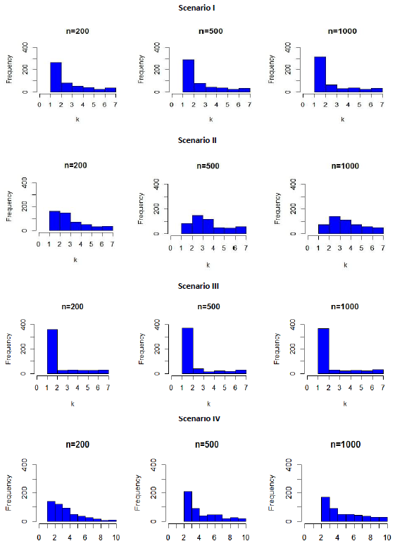
Figure 1: Histogram of $K$

The Monte Carlo sample size used to plot the histogram of $K$ is $J=500$.

7 Discussion

The data missing not at random problem is common in applications. Morikawa and Kim (2016) studies the efficient estimation of a class of missing not at random problems. But their approach requires nonparametric estimation of the conditional density function and thus suffers from the curse of dimensionality and smoothing parameter selection problem. In this paper, we study the same class of missing not at random problems but present a much simpler and more natural efficient estimator. Our approach is based on a parametric moment restriction model that does not require nonparametric estimation and hence does not suffer from the curse of dimensionality problem nor the bandwidth selection problem. Indeed the simulation results confirm that the proposed approach out-performs their approach in finite samples. The GMM approach is also easy to adapt to stratified sampling and other sampling schemes common in survey data.

Both approaches require correct parameterization of the propensity score function. If the propensity score function is misspecified, then both approaches yield inconsistent estimates. There is some attempt in the literature to mitigate this problem. For instance, Zhao and Shao (2015) introduce a partial linear index to model missing mechanism. The proposed approach can be extended in this direction. Such extension shall be pursued in a future study.

8 Appendix

8.1 Assumptions

We first introduce the smoothness classes of functions used in the nonparametric estimation; see e.g. Stone (1982, 1994), Robinson (1988), Newey (1997), Horowitz (2012) and Chen (2007). Suppose that $\mathcal{X}$ is the Cartesian product of $r$-compact intervals. Let $0<\delta\leq 1$. A fucntion $f$ on $\mathcal{X}$ is said to satisfy a H$\ddot{\text{o}}$lder condition with exponent $\delta$ if there is a positive constant $L$ usch that $\|f(\boldsymbol{x}_{1})-f(\boldsymbol{x}_{2})\|\leq L\|\boldsymbol{x}_{1}-\boldsymbol{x}_{2}\|^{\delta}$ for all $\boldsymbol{x}_{1},\boldsymbol{x}_{2}\in\mathcal{X}$. Given a $r$-tuple $\boldsymbol{\alpha}=(\alpha_{1},...,\alpha_{r})$ of nonnegative integer, denote $[\boldsymbol{\alpha}]=\alpha_{1}+\cdots+\alpha_{r}$ and let $D^{\boldsymbol{\alpha}}$ denote the differential operator defined by $D^{\boldsymbol{\alpha}}=\frac{\partial^{[\boldsymbol{\alpha}]}}{\partial x_{1}^{\alpha_{1}}\cdots\partial x_{r}^{\alpha_{r}}}$, where $\boldsymbol{x}=(x_{1},...,x_{r})$.

Definition 1.

Let $s$ be a nonnegative integer and $s:=s_{0}+\delta$. The function $f$ on $\mathcal{X}$ is said to be $s$-smooth if it is $s$ times continuously differentiable on $\mathcal{X}$ and $D^{\boldsymbol{\alpha}}f$ satisfies a H$\ddot{\text{o}}$lder condition with exponent $\delta$ for all $\boldsymbol{\alpha}$ with $[\boldsymbol{\alpha}]=s_{0}$.

The following notations are needed for presenting the efficiency bounds:

$$O(\boldsymbol{Z}):=\frac{1-\pi(\boldsymbol{Z};\gamma_{0})}{\pi(\boldsymbol{Z};\gamma_{0})},\text{\quad}\boldsymbol{S}_{0}(\boldsymbol{Z}):=-\frac{\nabla_{\gamma}\pi(\boldsymbol{Z};\gamma_{0})}{1-\pi(\boldsymbol{Z};\gamma_{0})}\ ,$$ (10)

$$m(\boldsymbol{X}):=\frac{\mathbb{E}[O(\boldsymbol{Z})\boldsymbol{S}_{0}(\boldsymbol{Z})|\boldsymbol{X}]}{\mathbb{E}[O(\boldsymbol{Z})|\boldsymbol{X}]},\text{\quad}R(\boldsymbol{X}):=\frac{\mathbb{E}[O(\boldsymbol{Z})U(\boldsymbol{Z})|\boldsymbol{X}]}{\mathbb{E}[O(\boldsymbol{Z})|\boldsymbol{X}]}\;\ ,$$ (11)

$$\boldsymbol{S}_{1}(T,\boldsymbol{Z};\gamma_{0}):=\left(1-\frac{T}{\pi(\boldsymbol{Z};\gamma_{0})}\right)m(\boldsymbol{X})\;\text{,}$$ (12)

$$S_{2}(T,\boldsymbol{Z};\gamma_{0},\theta_{0}):=-\frac{T}{\pi(\boldsymbol{Z};\gamma_{0})}U(\boldsymbol{Z})+\theta_{0}-\left(1-\frac{T}{\pi(\boldsymbol{Z};\gamma_{0})}\right)R(\boldsymbol{X})\;\text{.}$$ (13)

The following assumptions are required in this paper:

Assumption 1.

There exists a nonresponse instrumental variable $\mathbf{X}_{\mathbf{2}}$, i.e., $\mathbf{X}=(\mathbf{X}_{1}^{{}^{\intercal}},\mathbf{X}_{2}^{{}^{\intercal}})^{{}^{\intercal}}\text{,}$ such that $\boldsymbol{X}_{2}$ is independent of $T$ given $\boldsymbol{X}_{1}$ and $Y$; furthermore, $\boldsymbol{X}_{2}$ is correlated with $Y$.

Assumption 2.

The support of $\mathbf{X}$, which is denoted by $\mathcal{X}$, is a Cartesian product of $r$-compact intervals, and we denote $\boldsymbol{X}=(X_{1},...,X_{r})^{\top}$.

Assumption 3.

The functions $\mathbb{E}[O(\boldsymbol{Z})S_{0}(\boldsymbol{Z})|\mathbb{X}=\boldsymbol{x}]$, $\mathbb{E}[O(\boldsymbol{Z})U(\boldsymbol{Z})|\mathbb{X}=\boldsymbol{x}]$ and $\mathbb{E}[O(\boldsymbol{Z})|\boldsymbol{X}=\boldsymbol{x}]$ are $s$-smooth in $\boldsymbol{x}$, where $s>0$.

Assumption 4.

There exists two finite positive constants $\underline{a}$ and $\overline{a}$ such that the smallest (resp. largest) eigenvalue of $\mathbb{E}[u_{K}(\boldsymbol{X})u_{K}^{\top}(\boldsymbol{X})]$ is bounded away from $\underline{a}$ (resp. $\overline{a}$) uniformly in $K$, i.e.,

$$0<\underline{a}\leq\lambda_{\min}(\mathbb{E}[u_{K}(\boldsymbol{X})u_{K}(\boldsymbol{X})^{\top}])\leq\lambda_{\max}(\mathbb{E}[u_{K}(\boldsymbol{X})u_{K}(\boldsymbol{X})^{\top}])\leq\overline{a}<\infty\ .$$

Remark: Asssumption 4 implies that following results:

1. $$\mathbb{E}[\|u_{K}(\boldsymbol{X})\|^{2}]=\text{tr}\left(\mathbb{E}\left[u_{K}(\boldsymbol{X})u_{K}(\boldsymbol{X})^{\top}\right]\right)=O(K)\ ;$$ (14)

2. the matrices $\bar{a}\cdot I_{K\times K}-\mathbb{E}[u_{K}(\boldsymbol{X})u_{K}(\boldsymbol{X})^{\top}]$ and $\mathbb{E}[u_{K}(\boldsymbol{X})u_{K}(\boldsymbol{X})^{\top}]-\underline{a}\cdot I_{K\times K}$ are positive definite, and

   $$\underline{a}\leq\inf_{k\in\{1,...,K\}}\mathbb{E}[u_{kK}(\boldsymbol{X})^{2}]\leq\sup_{k\in\{1,...,K\}}\mathbb{E}[u_{kK}(\boldsymbol{X})^{2}]\leq\overline{a}\ .$$ (15)

Assumption 5.

The full data $\{(T_{i},\boldsymbol{X}_{i},Y_{i})\}_{i=1}^{N}$ are independently and identically distributed.

Assumption 6.

$\boldsymbol{S}_{eff}(T,\boldsymbol{Z};\gamma,\theta):=(\boldsymbol{S}_{1}^{{}^{\intercal}}(T,\boldsymbol{Z};\gamma),S_{2}(T,\boldsymbol{Z};\gamma,\theta))^{{}^{\intercal}}$ is continuously differentiable at each $(\gamma,\theta)\in\Gamma\times\Theta$ with probability one, and $\mathbb{E}\left[\partial\boldsymbol{S}_{eff}(\gamma,\theta)/\partial(\gamma^{\top},\theta)\right]$ is nonsingular at $(\gamma_{0},\theta_{0})$.

Assumption 7.

The response probability $\pi$ satisfies the following conditions:

1. there exists two positive constants $\bar{c}$ and $\underline{c}$ such that $0<\underline{c}\leq\pi(\boldsymbol{x},y;\gamma)\leq\bar{c}<1$ for all $\gamma\in\Gamma$ and $(\boldsymbol{x},y)\in\mathcal{X}\times\mathbb{R}$;

2. the propensity score $\pi(\boldsymbol{x},y;\gamma)$ is twice continuously differentiable in $\gamma\in\Gamma$, and the derivatives are uniformly bounded.

3. for any $\gamma\in\Gamma$, the conditional functions $\mathbb{E}\left[1-\frac{T}{\pi(\boldsymbol{Z};\gamma)}|\boldsymbol{X}=\boldsymbol{x}\right]$ and $\mathbb{E}\left[\frac{\nabla_{\gamma}\pi(\boldsymbol{Z};\gamma)}{\pi(\boldsymbol{Z};\gamma)}\bigg{|}\boldsymbol{X}=\boldsymbol{x}\right]$ are $s$-smooth in $\boldsymbol{x}$, where $s>0$.

Assumption 8.

Suppose $K\rightarrow\infty$ and $K^{3}/N\rightarrow 0$.

The Assumption 1 is used for the identification of the model, which was discussed in Wang et al. (2014). Assumptions 2 and 3 are required for uniform boundedness of approximations. Assumption 4 is a standard assumption used in nonparametric sieve approximation, see also Newey (1997). Assumption 5 is a standard condition for statistical sampling. Assumptions 6-7 are required for the convergence of our estimator as well as the boundness of the asymptotic variance. Assumption 8 is the same as Assumption 2 in Newey and Powell (2003), it is required for controlling the stochastic order of the residual terms, which is desirable in practice because $K$ grows very slowly with $N$ so a relatively small number of moment conditions is sufficient for the method proposed to perform well.

8.2 Discussion on $u_{K}$

To construct the GMM estimator, we need to specify the matching function $u_{K}(\boldsymbol{X})$. Although the approximation theory is derived for general sequences of approximating functions, the most common class of functions are power series. Suppose the dimension of covariate $\boldsymbol{X}$ is $r\in\mathbb{N}$, namely $\boldsymbol{X}=(X_{1},...,X_{r})^{\top}$. Let $\lambda=(\lambda_{1},\ldots\lambda_{r})^{\top}$ be an $r$-dimensional vector of nonnegative integers (multi-indices), with norm $|\lambda|=\sum_{j=1}^{r}\lambda_{j}$. Let $(\lambda(k))_{k=1}^{\infty}$ be a sequence that includes all distinct multi-indicesand satisfies $|\lambda(k)|\leq|\lambda(k+1)|$, and let $\boldsymbol{X}^{\lambda}=\prod_{j=1}^{r}X_{j}^{\lambda_{j}}$. For a sequence $\lambda(k)$ we consider the series $u_{kK}(\boldsymbol{X})=\boldsymbol{X}^{\lambda(k)}$, $k\in\{1,...,K\}$. Newey (1997) showed the following property for the power series: there exists a universal constant $C>0$ such that

$$\zeta(K):=\underset{\boldsymbol{x}\in\mathcal{X}}{\sup}\|u_{K}(\boldsymbol{x})\|\leq CK\ ,$$ (16)

where $\|\cdot\|$ denotes the usual matrix norm $\|A\|=\sqrt{\text{tr}(A^{\top}A)}$.

Another important issue is choosing the number of the matching function $K$ in finite sample experiment. Donald et al. (2009) proposed a strategy for an appropriate choice of $K$ by minimizing the higher order MSE defined in (9), and the following notations are needed to describe this criteria:

$$\rho(T_{i},\boldsymbol{X}_{i},Y_{i};\check{\gamma})=1-\frac{T_{i}}{\pi(\boldsymbol{X}_{i},Y_{i};\check{\gamma})},\text{\quad}\hat{\Upsilon}_{K\times K}=\frac{1}{N}\sum_{i=1}^{N}\rho(T_{i},\boldsymbol{X}_{i},Y_{i};\check{\gamma})^{2}u_{K}(\boldsymbol{X}_{i})^{\otimes 2}\text{,}$$

$$\widehat{\Gamma}_{K\times p}=\frac{1}{N}\sum_{i=1}^{N}u_{K}(\boldsymbol{X}_{i})\nabla_{\gamma}\rho(T_{i},\boldsymbol{X}_{i},Y_{i};\check{\gamma})^{\top},\text{\quad}\hat{\Omega}_{p\times p}=(\hat{\Gamma}_{K\times p})^{\top}\hat{\Upsilon}_{K\times K}^{-1}\hat{\Gamma}_{K\times p}\text{,}$$

$$\tilde{\mathbf{d}}_{i}=(\hat{\Gamma}_{K\times p})^{\top}\left(\frac{1}{N}\sum_{j=1}^{N}u_{K}(\boldsymbol{X}_{j})^{\otimes 2}\right)^{-1}u_{K}(\boldsymbol{X}_{i}),\text{\quad}\tilde{\mathbf{\eta}}_{i}=\nabla_{\gamma}\rho(T_{i},\boldsymbol{X}_{i},Y_{i};\check{\gamma})-\tilde{\mathbf{d}}_{i}\text{,}$$

$$\hat{\xi}_{ij}=\frac{1}{N}u_{K}(\boldsymbol{X}_{i})^{\top}\hat{\Upsilon}_{K\times K}^{-1}u_{K}(\boldsymbol{X}_{j}),\text{\quad}\widehat{\mathbb{D}}_{i}^{\ast}=(\hat{\Gamma}_{K\times p})^{\top}\hat{\Upsilon}_{K\times K}^{-1}u_{K}(\boldsymbol{X}_{i})\;\text{.}$$

8.3 Semiparametric Efficiency Bounds

The following lemma is Theorem 1 in Morikawa and Kim (2016).

Lemma 1 (Morikawa and Kim (2016)).

The efficient variance bounds of $(\gamma_{0},\theta_{0})$ is $\boldsymbol{V}_{eff}:=\mathbb{E}\left[\boldsymbol{S}_{eff}(T,\mathbb{Z};\gamma_{0},\theta_{0})^{\otimes 2}\right]^{-1}$, where $\boldsymbol{S}_{eff}=(\boldsymbol{S}_{1}^{\top},S_{2})^{\top}$ and $\boldsymbol{S}_{1}$, $S_{2}$ are defined in (12) and (13) respectively.

Let $\boldsymbol{V}_{\gamma_{0}}$ (resp. $V_{\theta_{0}}$) be the efficient variance bound of $\gamma_{0}$ (resp. $\theta_{0}$). After some simple computation, we can find out

$$\boldsymbol{V}_{\gamma_{0}}= \mathbb{E}\left[\frac{1-\pi(\boldsymbol{Z};\gamma_{0})}{\pi(\boldsymbol{Z};\gamma_{0})}m(\boldsymbol{X})^{\otimes 2}\right]^{-1}$$ (17)

and

$$V_{\theta_{0}}=Var\left(S_{2}(T,\boldsymbol{Z};\gamma_{0},\theta_{0})-\mathbf{\kappa}^{{}^{\intercal}}\boldsymbol{S}_{1}(T,\boldsymbol{Z};\gamma_{0})\right)\;\text{.}$$ (18)

where

$$\mathbf{\kappa}^{{}^{\intercal}}:=\mathbb{E}\left[\frac{\nabla_{\gamma}\pi(\boldsymbol{Z};\gamma_{0})^{{}^{\intercal}}}{\pi(\boldsymbol{Z};\gamma_{0})}\{R(\boldsymbol{Z})-U(\boldsymbol{X})\}\right]\cdot\mathbb{E}\left[\frac{m(\boldsymbol{X})}{\pi(\boldsymbol{Z};\gamma_{0})}\nabla_{\gamma}\pi(\boldsymbol{Z};\gamma_{0})^{{}^{\intercal}}\right]^{-1}\;\text{.}$$ (19)

References

• (1)
• Ai and Chen (2012) Ai, C. and Chen, X. (2012). The semiparametric efficiency bound for models of sequential moment restrictions containing unknown functions, Journal of Econometrics 170(2): 442–457.
• Ai et al. (2018) Ai, C., Linton, O. and Zhang, Z. (2018). Supplemental material for “a simple and efficient estimation method for models with nonignorable missing data”, Technical report .
• Bang and Robins (2005) Bang, H. and Robins, J. M. (2005). Doubly robust estimation in missing data and causal inference models, Biometrics 61(4): 962–973.
• Chen (2007) Chen, X. (2007). Large sample sieve estimation of semi-nonparametric models, Handbook of econometrics 6: 5549–5632.
• Chen et al. (2008) Chen, X., Hong, H. and Tarozzi, A. (2008). Semiparametric efficiency in gmm models with auxiliary data, Ann. Statist. 36(2): 808–843.
• Donald et al. (2009) Donald, S. G., Imbens, G. W. and Newey, W. K. (2009). Choosing instrumental variables in conditional moment restriction models, Journal of Econometrics 152(1): 28–36.
• Geman and Hwang (1982) Geman, S. and Hwang, C.-R. (1982). Nonparametric maximum likelihood estimation by the method of sieves, The Annals of Statistics pp. 401–414.
• Hansen (1982) Hansen, L. P. (1982). Large sample properties of generalized method of moments estimators, Econometrica: Journal of the Econometric Society pp. 1029–1054.
• Heitjan and Basu (1996) Heitjan, D. F. and Basu, S. (1996). Distinguishing “missing at random” and “missing completely at random”, The American Statistician 50(3): 207–213.
• Horowitz (2012) Horowitz, J. L. (2012). Semiparametric methods in econometrics, Vol. 131, Springer Science & Business Media.
• Kang and Schafer (2007) Kang, J. and Schafer, J. (2007). Demystifying double robustness: a comparison of alternative strategies for estimating a population mean from incomplete data, Statistical science 22(4): 523–539.
• Kim and Yu (2011) Kim, J. K. and Yu, C. L. (2011). A semiparametric estimation of mean functionals with nonignorable missing data, Journal of the American Statistical Association 106(493): 157–165.
• Little (1988) Little, R. J. (1988). A test of missing completely at random for multivariate data with missing values, Journal of the American Statistical Association 83(404): 1198–1202.
• Little and Rubin (1989) Little, R. J. and Rubin, D. B. (1989). The analysis of social science data with missing values, Sociological Methods & Research 18(2-3): 292–326.
• Little and Rubin (2014) Little, R. J. and Rubin, D. B. (2014). Statistical analysis with missing data, John Wiley & Sons.
• Morikawa and Kim (2016) Morikawa, K. and Kim, J. K. (2016). Semiparametric adaptive estimation with nonignorable nonresponse data, arXiv preprint arXiv:1612.09207 .
• Newey (1997) Newey, W. K. (1997). Convergence rates and asymptotic normality for series estimators, Journal of econometrics 79(1): 147–168.
• Newey and Powell (2003) Newey, W. K. and Powell, J. L. (2003). Instrumental variable estimation of nonparametric models, Econometrica 71(5): 1565–1578.
• Newey and Smith (2004) Newey, W. K. and Smith, R. J. (2004). Higher order properties of gmm and generalized empirical likelihood estimators, Econometrica 72(1): 219–255.
• Qin et al. (2002) Qin, J., Leung, D. and Shao, J. (2002). Estimation with survey data under nonignorable nonresponse or informative sampling, Journal of the American Statistical Association 97(457): 193–200.
• Qin and Zhang (2007) Qin, J. and Zhang, B. (2007). Empirical-likelihood-based inference in missing response problems and its application in observational studies, J. R. Statist. Soc. B (Statistical Methodology) 69(1): 101–122.
• Riddles et al. (2016) Riddles, M. K., Kim, J. K. and Im, J. (2016). A propensity-score-adjustment method for nonignorable nonresponse, Journal of Survey Statistics and Methodology 4(2): 215–245.
• Robins et al. (1997) Robins, J. M., Ritov, Y. et al. (1997). Toward a curse of dimensionality appropriate(coda) asymptotic theory for semi-parametric models, Statistics in medicine 16(3): 285–319.
• Robins and Rotnitzky (1995) Robins, J. M. and Rotnitzky, A. (1995). Semiparametric efficiency in multivariate regression models with missing data, Journal of the American Statistical Association 90(429): 122–129.
• Robins et al. (1995) Robins, J. M., Rotnitzky, A. and Zhao, L. P. (1995). Analysis of semiparametric regression models for repeated outcomes in the presence of missing data, Journal of the american statistical association 90(429): 106–121.
• Robinson (1988) Robinson, P. M. (1988). Root-n-consistent semiparametric regression, Econometrica: Journal of the Econometric Society pp. 931–954.
• Rotnitzky et al. (2012) Rotnitzky, A., Lei, Q., Sued, M. and Robins, J. M. (2012). Improved double-robust estimation in missing data and causal inference models, Biometrika 99(2): 439–456.
• Rubin (1976a) Rubin, D. B. (1976a). Comparing regressions when some predictor values are missing, Technometrics 18(2): 201–205.
• Rubin (1976b) Rubin, D. B. (1976b). Inference and missing data, Biometrika 63(3): 581–592.
• Shao and Wang (2016) Shao, J. and Wang, L. (2016). Semiparametric inverse propensity weighting for nonignorable missing data, Biometrika 103(1): 175–187.
• Stone (1982) Stone, C. J. (1982). Optimal global rates of convergence for nonparametric regression, The annals of statistics pp. 1040–1053.
• Stone (1994) Stone, C. J. (1994). The use of polynomial splines and their tensor products in multivariate function estimation, The Annals of Statistics pp. 118–171.
• Sverchkov (2008) Sverchkov, M. (2008). A new approach to estimation of response probabilities when missing data are not missing at random, Proceedings of the Survey Research Methods Section, pp. 867–874.
• Tan (2010) Tan, Z. (2010). Bounded, efficient and doubly robust estimation with inverse weighting, Biometrika 97(3): 661–682.
• Tang et al. (2003) Tang, G., Little, R. J. and Raghunathan, T. E. (2003). Analysis of multivariate missing data with nonignorable nonresponse, Biometrika 90(4): 747–764.
• Wang et al. (2014) Wang, S., Shao, J. and Kim, J. K. (2014). An instrumental variable approach for identification and estimation with nonignorable nonresponse, Statistica Sinica pp. 1097–1116.
• Zhao and Shao (2015) Zhao, J. and Shao, J. (2015). Semiparametric pseudo-likelihoods in generalized linear models with nonignorable missing data, Journal of the American Statistical Association 110(512): 1577–1590.