On the edge energy of graphene

Abstract

Surface/edge energy is typically modeled as a continuous function of orientation, $\gamma({\bf n})$. We put forward a simple geometric argument that suggests this picture is inadequate for crystals with a non-Bravais lattice structure. In the case of the idealized graphene/hexagonal lattice, our arguments indicate that the edge energy can be viewed as both discontinuous and multi-valued for a subset of orientations that are commensurate with the crystal structure.

Surface/edge energy is normally modeled as a continuous function of surface/edge orientation, $\gamma(\hat{{\bf n}})$ langer ; BWBK . This function is often constructed so that it is consistent with underlying symmetry constraints combined with experimental observations or data from computations elder ; MBW . In this paper, we put forward a simple geometric argument that suggests this picture is incomplete for crystals with a non-Bravais lattice structure. Instead, we argue that when such a crystal is cleaved by an arbitrarily positioned plane or line, the resulting surface energy can be both multivalued and discontinuous when viewed as a function of orientation. This is due to the fact that that some orientations give rise to a translation invariant surface energy, while others do not.

These singularities occur for a discrete set of orientations that are commensurate with the crystal structure. In the case of graphene, this includes the so-called “zigzag” orientation, which is often found to dominate the equilibrium shape of isolated graphene crystals. While we expect similar conclusions to apply to real materials and first-principles calculations, including graphene films grown on substrates, we examine these effects for an isolated hexagonal lattice using nearest-neighbor, bond-counting arguments, neglecting reconstructions and other off-lattice effects. The surface energy we discuss throughout most of the paper corresponds to the zero-temperature energy landscape of an ideal bulk-truncated surface/edge.

In a pairwise bond-counting model, an energy is defined for a given lattice configuration by defining sets of bond orientations ${\rm V}=\{\{{\bf v}_{ij}\}_{j=1}^{J_{i}}\}_{i=1}^{N_{p}}$ and corresponding bond energies $e_{ij}$ for each of the $N_{p}$ particles in the system MMN . These sets are often restricted to neighboring pairs of atoms, but, in principle, could include all combinations of atoms. For our nearest-neighbor hexagonal/graphene model, the particles have one of two distinct sets of bonds, $\{\{{\bf v}_{Aj}\}_{j=1}^{3},\{{\bf v}_{Bj}\}_{j=1}^{3}\}$. For a crystal with a Bravais lattice structure, the same set of bonds, $\{\mathbf{v}_{j}\}_{j=1}^{J}$, applies to each particle in the crystal. The surface/edge energy of bond-counting models on Bravais lattices is given by

$$\gamma(\hat{\mathbf{n}})=\frac{1}{2}\sum_{j=1}^{J}e_{j}\frac{|\hat{\mathbf{n}}\cdot\mathbf{v}_{j}|}{|\det A|}$$ (1)

where $\hat{\mathbf{n}}$ is the normal to the surface/edge and $A$ is a matrix with the lattice primitive vectors as columns herr .

The idealized graphene structure is one of the simplest examples of a non-Bravais lattice. Gan and Srolovitz were the first to address the issue of edge energy for individual graphene flakes GS . They use DFT calculations for a collection of graphene ribbons at seven different orientations to interpolate an edge energy function, and consider unreconstructed graphene with both non-terminated and hydrogen terminated bonds, as well as a model for reconstructed graphene. Liu et al. LDY revisit the problem and first consider an arbitrarily oriented graphene edge that can be decomposed into a number of “zigzag” and “armchair” components, so that the edge energy can be represented using two energies of these primary configurations along with zigzag and armchair densities that can be computed from simple geometric considerations:

$$\gamma(\chi)=\frac{4}{\sqrt{3}}\epsilon_{A}\sin(\chi)+2\epsilon_{Z}\sin(\pi/6-\chi),$$

where $\epsilon_{A}$ and $\epsilon_{Z}$ are the energies of an atom in an armchair or zigzag component respectively and $\chi$ is the edge angle. This assumption is equivalent to assuming edges of the graphene flake do not contain singly-bonded carbon-atoms. This same assumption appears to have been tacitly made in GS , as a perfectly linear edge with the slope indicated in their Fig. 2b would have an additional singly-bonded atom at the kinks along the edge. For the graphene structure, we will see that including such atoms leads to a discontinuous, multi-valued edge energy.

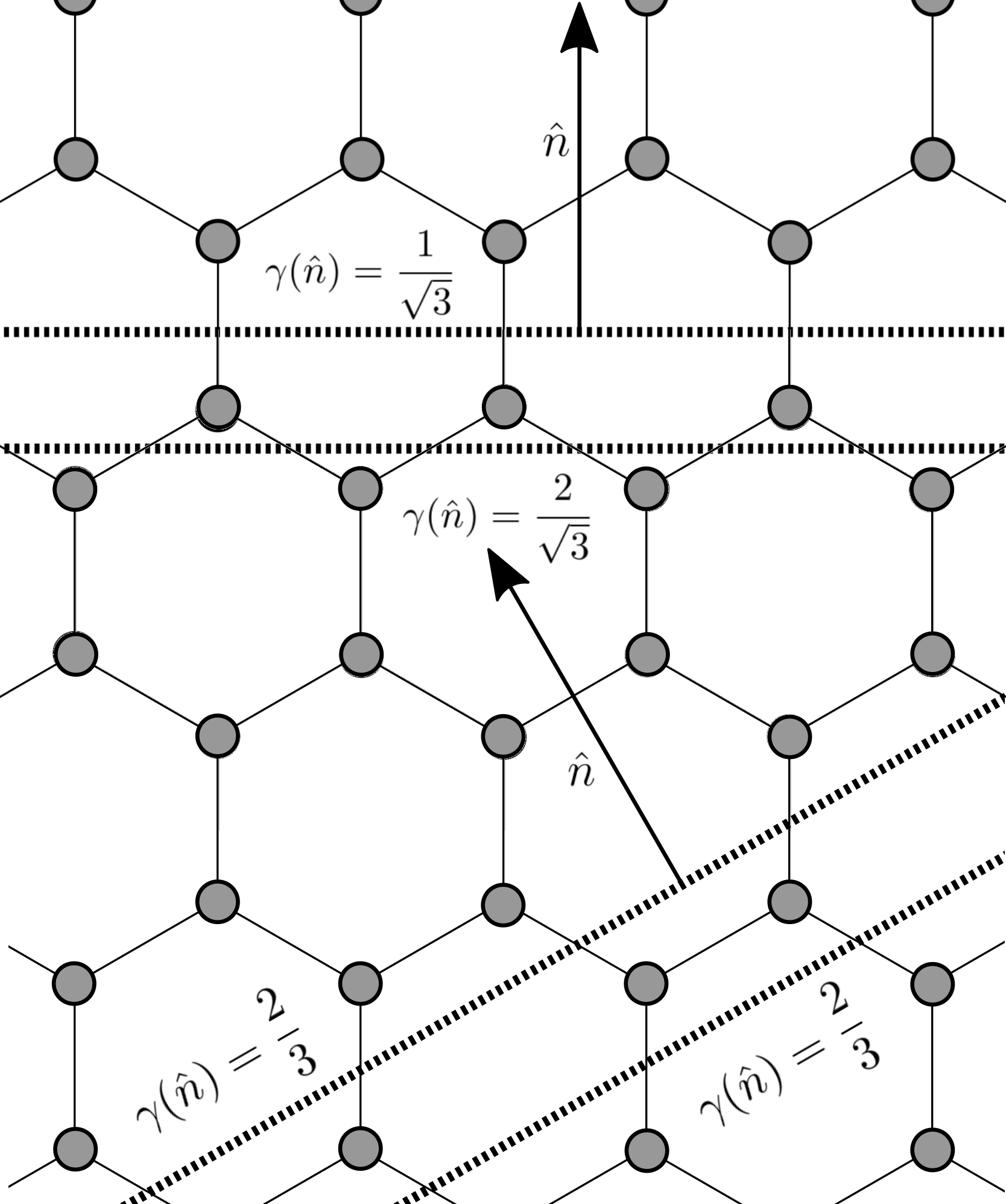
Figure 1: A hexagonal/graphene lattice cut by two lines in the zigzag orientation (near the top of the figure) and two more in the armchair orientation (near the bottom of the figure). In the case of the zigzag orientations, the broken bond density can be altered by a parallel translation of the edge, while the broken bond density is translation invariant for the armchair orientation.

While it is not surprising that equilibrium shapes are dominated by facets without these dangling atoms, it seems clear they would appear in non equilibrium structures and could affect the dynamics of relaxation and growth processes. Indeed, Liu et al. go on to consider growth mechanisms involving singly-bonded carbon atoms arriving at and diffusing along steps similar to what occurs in the traditional Burton-Cabrera-Frank BCF theory of step-flow on surfaces , and singly-bonded atoms at graphene edges have been observed in experiments SK . In view of this, we examine a more complete picture of surface/edge energy as a function of perfectly planar/linear facets at arbitrary orientations and positions.

The mechanism that is responsible for the discontinuities in the surface energy is illustrated in Figure 1 using a nearest-neighbor bonded crystal with the hexagonal/graphene structure. Most facets behave like the armchair orientation shown at the bottom of Figure 1, where the broken bond density, which represents edge energy in this simple model, is translation invariant. This contrasts with a countable, discrete set of orientations that behave like the zig-zag orientation shown at the top of Figure 1, where the broken bond density alternates between two values as the line cutting the crystal is translated in the normal direction.

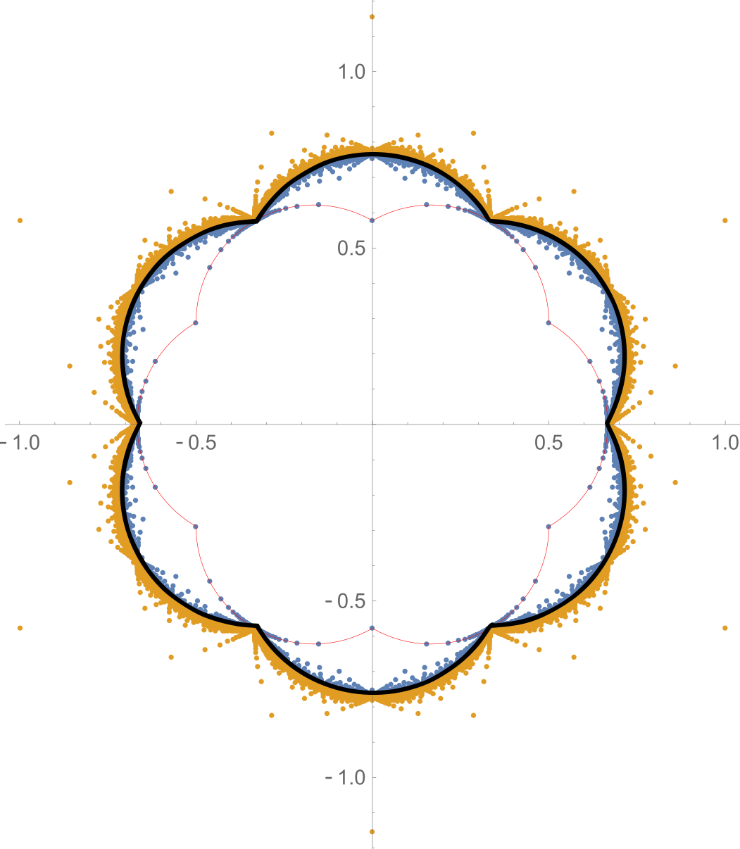
(a)

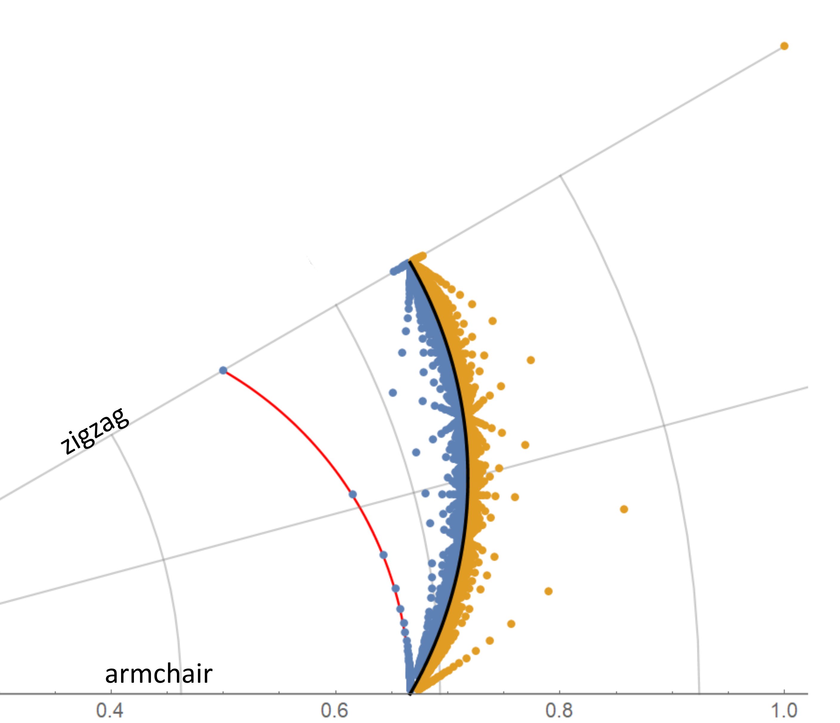
(b)

Figure 2: A polar plot of broken-bond density/edge energy for the hexagonal/graphene crystal as a function of edge orientation. The entire plot is shown in (a) while (b) contains only the wedge ranging between armchair and zigzag orientations. Most values lie on the black curve, while the discrete set of incongruent orientations gives rise to discontinuities with two edge energy values for each orientation: the minimum values are shown in blue and the maximum values are gold. The red curve interpolates between the zigzag and armchair orientation by neglecting dangling bonds.

In general, edge orientations fall into one of two categories: commensurate orientations result in a periodic pattern of broken bonds, while non-commensurate orientations result in an aperiodic pattern of broken bonds. An edge with a commensurate orientation can be translated so that it passes through multiple sites, while an edge with an incommensurate orientation can pass through at most one site. The commensurate edges give rise to two subcases we refer to as congruent and incongruent. While the incommensurate and congruent orientations have translation invariant edge energies, the edge energy for the incongruent orientations is multi-valued. An edge with a congruent orientation can be translated so that it passes through either no sites or sites with both A-oriented and B-oriented bonds, alternating between the two, while an edge with an incongruent orientation can only pass through no sites or sites with the same bond orientations.

These results are summarized in Figure 2. The black curve is the edge energy that applies to the uncountably infinite number of incommensurate and the countably infinite set of congruent edges. This edge energy is exactly $1/3$ what one would find for a nearest neighbor model based on the related Bravais lattice with an additional lattice point in the center of each hexagon. This curve is discontinuous at the incongruent orientations, where one finds two possible values of the edge energy depending on the placement of the facet in the normal direction. It can be shown that the average of these two values again lies on the black curve. Finally, the red curve is the edge energy derived in Liu et al. LDY by assuming edges that consist of only armchair and zigzag components. This curve is a lower bound on the edge energy, and is formed by continuously interpolating between the lower of the two possible values one can obtain with a zigzag orientation and the single value for the armchair orientation. Note that if this simple, interpolated edge energy function was used to evolve a non-equilibrium shape, one would not expect any qualitative difference in the dynamics compared to that for a material with a triangular lattice structure, i.e. both edge energies are a six-petaled flower.

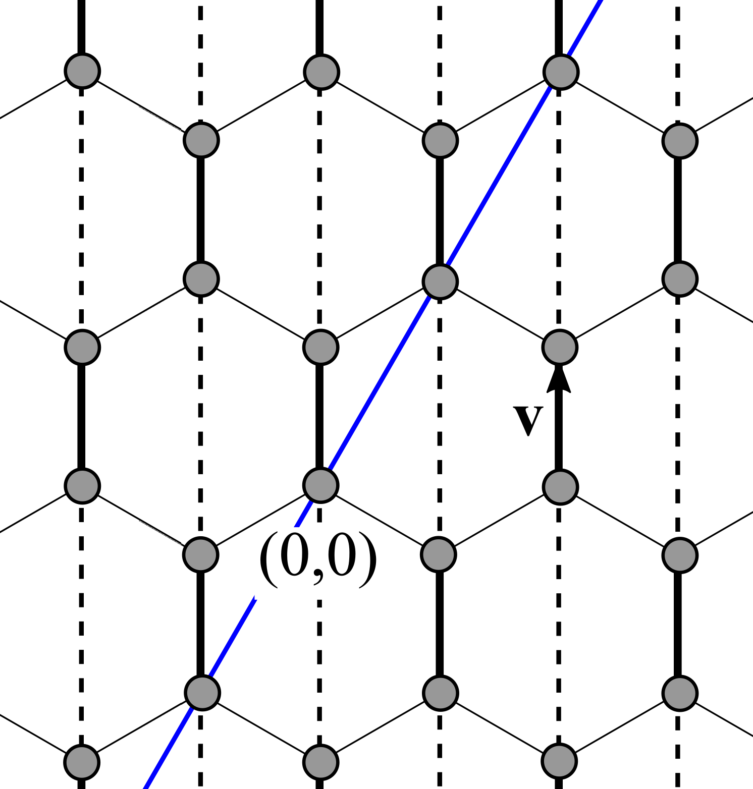
Figure 3: The hexagonal lattice with a single nearest-neighbor bond $\mathbf{v}$ and its corresponding set of bondlines. The blue reference line $\hat{y}=\sqrt{3}x$ is used to define the sequence $\delta_{n}$ referred to in the text.

To get these results, we follow arguments that generalize those of Mackenzie et. al. MMN , i.e. we compute a contribution to the edge energy for each bond orientation ${\bf v}$ and sum the result over all bonds $V$. To this end, consider the set of all bond-lines parallel to $\mathbf{v}$ that pass through lattice sites. Note that the bonds only cover $\frac{1}{3}$ of each bond-line, with a repeating pattern of one bond followed by two bond-less segments (see Figure 3). Thus, the bonds and bond-line structure are periodic in the vertical direction with period $3a$, where $a$ is the bond length. We will make use of a Cartesian coordinate system where the y-axis is aligned with the bond and the origin is placed at the lower end of an arbitrary bond. It is also convenient to introduce a reference line $\hat{y}=\sqrt{3}x$ and measure distance in the direction of $\mathbf{v}$ relative to this line, $\Delta=y-\hat{y}$.

Next, we consider an arbitrary edge $y=sx+b$ with slope $s$ and intercept $b$. Between any two adjacent bond-lines, this line rises a distance $r=\frac{\sqrt{3}}{2}as$ and intersects the $n^{th}$ bond-line, given by $x=n\frac{\sqrt{3}}{2}a$, at $y_{n}=rn+b$. Relative to the reference line defined above, this produces the sequence $\Delta_{n}=y_{n}-\hat{y}_{n}=(r-\frac{3a}{2})n+b$. We will need to consider y-values mapped to the interval $[0,3a]$ via congruence modulo $3a$. It will therefore be convenient to scale distance so that $a=\frac{1}{3}$ and this congruence operation corresponds to taking the fractional part of y-values. After scaling, half of the bonds are congruent to the interval $[0,1/3]$ while the other half are congruent to the interval $[1/2,5/6]$. Relative to the reference line, the scaled bond locations will have fractional parts in the interval $[0,1/3]$. In order to determine the intersections with bonds, it is sufficient to consider the fractional part of the sequence $\delta_{n}={\mbox{Frac}(\Delta_{n})}$.

An edge orientation is commensurate with respect to bond $\mathbf{v}$ if $r\in\mathbb{Q}$ and incommensurate otherwise. For a given edge orientation, one can show that all of the bonds $\mathbf{v}\in V$ fall into the same category. For incommensurate orientations, the edge energy is defined as the mean number of bonds cut across the entire edge. A natural hypothesis for this mean is $\gamma(\hat{\mathbf{n}})=\frac{1}{3}\Gamma(\hat{\mathbf{n}})$, where $\Gamma$ is the edge energy for the related triangular lattice with additional nodes in the center of each hexagon, as the graphene lattice is formed by removing $\frac{2}{3}$ of these bonds. The triangular lattice is Bravais, so that $\Gamma$ can be computed from (1).

To see that this is correct, we first consider the case $b=0$, producing the sequence $\delta_{n}=\mbox{Frac}[(r-\frac{1}{2})n]$. Since $r$ is irrational, so is $r-\frac{1}{2}$ and Weyl’s equidistribution theorem weyl then indicates that the sequence is uniformly distributed. This implies that one third of the bond-line intersections correspond to broken bonds. For $b\neq 0$, $\mbox{Frac}[(r-\frac{1}{2})n+b]=\mbox{Frac}[(r-\frac{3a}{2})n+\mbox{Frac}(b)]$, from which we can see that broken bond density in the incommensurate case is translation invariant, as the portion of the uniform distribution of $\delta_{n}$ that is shifted out of the interval $[0,1]$ on the right simply reemerges on the left. The same result holds for each $\mathbf{v}\in{\rm V}$ and therefore

$$\gamma(\hat{\mathbf{n}})=\frac{1}{3}\Gamma(\hat{\mathbf{n}})=\frac{2}{3\sqrt{3}}\sum_{i=1}^{3}|\hat{\mathbf{n}}\cdot\mathbf{v}_{i},|$$ (2)

where we have expressed the result using twice the contribution from the three distinct A-bond orientations $\mathbf{v}_{A1}=(\sqrt{3}/2,1/2),\mathbf{v}_{A2}=(-\sqrt{3}/2,1/2),\mathbf{v}_{A3}=(0,1)$, as the B-bonds give rise to the same contributions.

The sequence $\delta_{n}$ is periodic whenever $r$ is rational, repeating every $N$ bond-lines, where $N$ is the smallest even integer such that $Nr\in\mathbb{Z}$. When this integer $N$ is divisible by three, we refer to the orientation as congruent, as one can show that congruence applies to all bonds $\mathbf{v}\in V$ or none at all. Congruent orientations have the same translation invariant broken bond density as the incommensurate orientations. To see this, note that the $N$ bond-line intersections are evenly spaced over one period of length $p=rN$ and that the corresponding values of $\delta_{n}$, though re-ordered, are uniformly spaced over the interval $[0,1]$, with one third of these corresponding to a bond crossing.

The remaining commensurate cases have a repeating sequence $\delta_{n}$ with $N\equiv 1$ or $2\mod 3$. In these cases, which we refer to as incongruent, there is no way to have exactly one third of the $\delta_{n}$ falling into the first third of $(0,1]$. Instead, the number of intersections with bonds per period will round up or down to the nearest integer that is divisible by 3. If $N\equiv 1\mod 3$, the lesser of the two edge energies is given by

$$\gamma_{\mathbf{v}}^{-}(\hat{\mathbf{n}})=\frac{n-1}{3p}=\frac{p\Gamma_{\mathbf{v}}(\hat{\mathbf{n}})-1}{3p}=\frac{1}{3}\Gamma_{\mathbf{v}}(\hat{\mathbf{n}})-\frac{1}{3p},$$

and the greater of the two edge energies is

$$\gamma_{\mathbf{v}}^{+}(\hat{\mathbf{n}})=\frac{1}{3}\Gamma_{\mathbf{v}}(\hat{\mathbf{n}})+\frac{2}{3p}.$$

Which of the two applies depends on the intercept $b$ of the dividing line, and the edge energy fails to be translation invariant for these orientations. The transition between the two values takes place whenever the edge crosses a lattice site. If $N\equiv 1\mod 3$, this occurs whenever $\text{Frac}(b)=k/N$ or $k/N+1/(3N)$ with $k\in\mathbb{Z}$. And if $N\equiv 2\mod 3$, when $\text{Frac}(b)=k/N$ or $k/N+2/(3N)$. We will refer to the set of edges with $b$ between any two of these transition values as a band. Note that all edges within a single band share the same energy value. There are two possible values for any edge orientation, with bands alternating between the two and one of the bands being twice as wide as the other.

If $N\equiv 2\mod 3$, the two edge energy values are

$$\gamma_{\mathbf{v}}^{-}(\hat{\mathbf{n}})=\frac{1}{3}\Gamma_{\mathbf{v}}(\hat{\mathbf{n}})-\frac{2}{3p},\;\gamma_{\mathbf{v}}^{+}(\hat{\mathbf{n}})=\frac{1}{3}\Gamma_{\mathbf{v}}(\hat{\mathbf{n}})+\frac{1}{3p}.$$

The total edge energy for an edge within a thin band is given by

$$\gamma_{1}(\hat{\mathbf{n}}) = \sum_{N\equiv 1\bmod 3}\gamma_{\mathbf{v}_{i}}^{+}(\hat{\mathbf{n}})+\sum_{N\equiv 2\bmod 3}\gamma_{\mathbf{v}_{i}}^{-}(\hat{\mathbf{n}})$$ (3)

$$= \frac{1}{3}\Gamma(\hat{\mathbf{n}})+\frac{2}{3p}(m_{1}-m_{2})$$

where $m_{j}$ is the number of bonds in $\{\mathbf{v}_{i}\}$ for which $N\equiv j\bmod 3$. Similarly, the edge energy for a edge within a thick band is

$$\gamma_{2}(\hat{\mathbf{n}})=\frac{1}{3}\Gamma(\hat{\mathbf{n}})+\frac{1}{3p}(m_{2}-m_{1}).$$ (4)

Note that

$$\lim_{p\rightarrow\infty}\gamma_{1}=\lim_{p\rightarrow\infty}\gamma_{1}=\frac{1}{3}\Gamma,$$

so that in the limit where the period of the bond intersections becomes large, both of the values for the incongruent orientations converge to the value for incommensurate/congruent orientations.

Let $\gamma^{-}(\hat{\mathbf{n}})=\min\{\gamma_{1}(\hat{\mathbf{n}}),\gamma_{2}(\hat{\mathbf{n}})\}$ and $\gamma^{+}(\hat{\mathbf{n}})=\max\{\gamma_{1}(\hat{\mathbf{n}}),\gamma_{2}(\hat{\mathbf{n}})\}$. These two functions are then the minimum and maximum energy values for the orientation $\hat{\mathbf{n}}$ shown in Figure 2. In particular, the zigzag orientations minimize $\gamma^{-}$ over all incongruent orientations. If we perform the classical Wulff construction using $\gamma^{-}$ as the edge energy, we get a hexagon with zigzag orientation edges, coinciding with the graphene equilibrium shape.

Further work examining the impact of these observations on the nonequilibrium evolution of crystals would be of interest. In particular, one would like to know if arbitrarily shaped crystals with a hexagonal/graphene crystal structure exhibit behavior that is qualitatively distinct from identically shaped crystals with a triangular lattice structure. A possible mechanism for such differences may be provided by the fact that a perturbation to the energy minimizing orientation for the hexagonal/graphene crystal will give rise to a jump in the edge energy, while a perturbation for the energy minimizing orientation for a crystal with a Bravais lattice structure will not. Simulations using molecular dynamics, kinetic Monte Carlo and/or phase-field crystal would seem well suited to exploring this possibility.

- (1) J. S. Langer, “Models of Pattern Formation in First-Order Phase Transitions”, Dir. Cond. Matt. Phys. 1 165–86 (1986).
- (2) W. J. Boettinger, J. A. Warren, C. Beckermann, and A. Karma, “Phase-Field Simulation of Solidification”, Annu. Rev. of Mater. Res. 32, 163–94 (2002).
- (3) N. Provatas and K. Elder, “Phase-Field Methods in Materials Science and Engineering”, Wiley (2001).
- (4) N. Moelans, B. Blanpain, and P. Wollants, “An introduction to phase-field modeling of microstructure evolution”, Calphad 32, 268–94 (2008).
- (5) J.K. Mackenzie, A.J.W. Moore, and J.F. Nicholas, “Bonds Broken at Atomically Flat Crystal Surfaces I: Face-Centered and Body-Centered Cubic Crystals”, J. Phys. Chem. Solids 23, 185–196 (1962).
- (6) C. Herring, “Some Theorems on the Free Energies of Crystal Surfaces”, Phys. Rev. 82 87–93 (1951).
- (7) C. K. Gan and D. Srolovitz, “Trends in graphene edge properties and flake shapes: a first-principles study”, Phys. Rev. B 81 125445 (2010).
- (8) Y. Liu, A. Dobrinsky, and B. Yakobson, “Graphene Edge from Armchair to Zigzag: The Origins of Nanotube Chirality?”, Phys. Rev. Lett. 105 235502 (2010).
- (9) W. K. Burton, N. Cabrera, and F. C. Frank “The Growth of Crystals and the Equilibrium Structure of their Surfaces”, Phil. Trans. R. Soc. Lond. A 243 299–358 (1951).
- (10) K. Suenaga and M. Koshino, “Atom-by-atom spectroscopy at graphene edge”, Nature 468, 1088–1090 (2010).
- (11) H. Weyl, “Ueber die Gleichverteilung von Zahlen mod.”, Math. Ann. 77, 313–352 (1916).
- (12) T. P. Schulze, “Morphological instability during directional epitaxy”, J. Crystal Growth, 295 188–201 (2006).