Chemical and Physical Picture of IRAS 16293–2422 Source B at a Sub-arcsecond Scale Studied with ALMA

Abstract

We have analyzed the OCS, H₂CS, CH₃OH, and HCOOCH₃ data observed toward the low-mass protostar IRAS 16293–2422 Source B at a sub-arcsecond resolution with ALMA. A clear chemical differentiation is seen in their distributions; OCS and H₂CS are extended with a slight rotation signature, while CH₃OH and HCOOCH₃ are concentrated near the protostar. Such a chemical change in the vicinity of the protostar is similar to the companion (Source A) case. The extended component is interpreted by the infalling-rotating envelope model with a nearly face-on configuration. The radius of the centrifugal barrier of the infalling-rotating envelope is roughly evaluated to be ($30-50$) au. The observed lines show the inverse P-Cygni profile, indicating the infall motion with in a few 10 au from the protostar. The nearly pole-on geometry of the outflow lobes is inferred from the SiO distribution, and thus, the infalling and outflowing motions should coexist along the line-of-sight to the protostar. This implies that the infalling gas is localized near the protostar and the current launching points of the outflow have an offset from the protostar. A possible mechanism for this configuration is discussed.

1 Introduction

IRAS 16293–2422 is a well-studied Class 0 protostellar source in Ophiuchus ($d=120$ pc) (Knude & Hog, 1998). This source is known to be a binary, consisting of Source A and Source B, whose apparent separation is 5″ ($\sim$600 au; e.g. Wootten, 1989; Mundy et al., 1992; Bottinelli et al., 2004). Molecular gas distribution and dynamics around the binary components have extensively been studied at a high angular resolution with millimeter- and submillimeter-wave interferometers (e.g. Mundy et al., 1992; Bottinelli et al., 2004; Kuan et al., 2004; Pineda et al., 2012; Zapata et al., 2013; Favre et al., 2014; Jørgensen et al., 2011, 2016). This source is also famous as a prototypical hot corino source, which is characterized by rich complex organic molecules (COMs) in the vicinity of the protostars (e.g. Schöier et al., 2002; Cazaux et al., 2003; Bottinelli et al., 2004; Kuan et al., 2004; Pineda et al., 2012; Jørgensen et al., 2012, 2016; Coutens et al., 2016).

Recently, ALMA Cycle 1 archival data toward this source was analyzed to investigate the kinematic structure of the infalling-rotating envelope associated with Source A by Oya et al. (2016). The authors found that the kinematic structure of the infalling-rotating envelope is successfully explained by a simple ballistic model (Oya et al., 2014). Based on this study, the radius of the centrifugal barrier of the infalling-rotating envelope was evaluated to be $\sim$50 au. Since the centrifugal barrier in the infalling-rotating envelope is also identified in other low-mass protostellar sources, L1527, TMC-1A, L483, BHB07-11, and HH212 (Sakai et al., 2014a, b, 2016, 2017; Oya et al., 2015, 2017; Alves et al., 2017; Lee et al., 2017), it seems to be a common occurrence in low-mass star formation.

In addition, a salient result of the above study (i.e. Oya et al., 2016) is that a drastic chemical change was found around the centrifugal barrier; the OCS (carbonyl sulphide) and H₂CS (thioformaldehyde) lines trace the infalling-rotating envelope outside the centrifugal barrier, while the COM lines, such as CH₃OH (methanol) and HCOOCH₃ (methyl formate), mainly highlight the centrifugal barrier. The H₂CS lines also trace the high velocity component inside the centrifugal barrier, which is likely a circumstellar disk component. Such enhancement of the COM emission around the centrifugal barrier would be an essential part of the hot corino chemistry in this source. Recently, a similar distribution of COMs around the centrifugal barrier is also reported for the low-mass protostellar source HH212 by Lee et al. (2017). Thus, the centrifugal barrier seems to stand for not only the physical transition zone from the infalling-rotating envelope to the disk, but also the transition zone of the chemical composition. Although the species tracing each part is different, chemical changes around centrifugal barriers are reported for other sources, L1527, TMC-1A, and L483 (Sakai et al., 2014b, 2016; Oya et al., 2017). Conversely, chemical diagnostics can be a powerful method to investigate the physical structure of the gas around a protostar at a 100 au scale.

In this study, we apply the chemical diagnostics to IRAS 16293–2422 Source B, which is the other component of the binary system. Source B is known to be rich in COMs as well as Source A (e.g. Bottinelli et al., 2004; Kuan et al., 2004; Jørgensen et al., 2011, 2012, 2016; Pineda et al., 2012). Its disk/envelope system is reported to have a nearly face-on geometry in contrast to the edge-on geometry of Source A (e.g. Pineda et al., 2012; Zapata et al., 2013; Oya et al., 2016). For this reason, the molecular line emission shows a narrower linewidth toward Source B than toward Source A. Furthermore, an inverse P-Cygni profile is reported toward Source B (e.g. Pineda et al., 2012; Jørgensen et al., 2012), which implies the existence of the infalling gas in front of the protostar along the line-of-sight. In this study, we analyze molecular distributions and the kinematic structure of this source at a sub-arcsecond resolution, and compare the results with those of Source A.

2 Observations

In this study, we used the ALMA Cycle 1 archival data of IRAS 16293–2422 in Band 6 (#2012.1.00712.S), which covers the frequency ranges from 230 to 250 GHz and from 220 to 240 GHz. The details of the observations are reported by Jørgensen et al. (2016) and Oya et al. (2016). Here, we briefly summarize important points. In the observations, (42–44) antennas were used, and the primary beam (half-power beam width) is (24–25)″. The largest recoverable scale is $\sim$13″ at 240 GHz. The backend correlator was tuned to a resolution of 122 kHz, which corresponds to the velocity resolution of 0.15 km s^-1 at 240 GHz, and a bandwidth of 468.750 MHz. The data calibration was performed in the antenna-based manner and uncertainties are less than 10 % (ALMA Cycle 1 Technical Handbook; Lundgren, 2012).

In addition, we also analyzed the ALMA Cycle 3 data, which were carried out on 5 March 2016 (#2015.1.01060.S). 41 antennas were used in these observations with the baseline length ranging from 17 to 636 m. The largest recoverable scale is $\sim$14″ at 260 GHz. The phase center of these observations is ($\alpha_{2000}$, $\delta_{2000}$) = ($16^{\rm h}32^{\rm m}22\fs 87$, $-24\arcdeg 28\arcmin 36\farcs 3$), and the primary beam is 25″. The total on-source time was 16.38 minutes with typical system temperature of (60–140) K. The backend correlator was tuned to a resolution of 122 kHz, which corresponds to the velocity resolution of 0.14 km s^-1 at 260 GHz, and a bandwidth of 58.6 MHz. J1625-2527 was used for the phase calibration. The bandpass calibration was done on the quasar J1427-4206, and the absolute flux density scale was derived from Titan. The data calibration was performed in the antenna-based manner, and uncertainties are less than 10 % (ALMA Cycle 3 Technical Handbook; Remijan et al., 2015).

Observed spectral lines are summarized in Table 1, including their rest frequencies, upper state energies, intrinsic line strengths, and synthesized beams. The 1.3 mm (236 GHz) continuum image was obtained by averaging the line-free channels of the two Cycle 1 data (230 and 240 GHz), whose total band width is 7.5 GHz. The line images were obtained by subtracting the continuum data directly from the visibilities. The Brigg’s weighting with the robustness parameter of 0.5 was employed to obtain the images of the continuum and the spectral lines. Self-calibration using the continuum emission was applied to the ALMA Cycle 1 data (the continuum, OCS, CH₃OH, HCOOCH₃, and H₂CS). On the other hand, it was not applied to the ALMA Cycle 3 data (SiO), because the continuum sensitivity is not enough for self-calibration processing due to a limited number of line-free channels.

3 Distribution

3.1 Overall Distributions

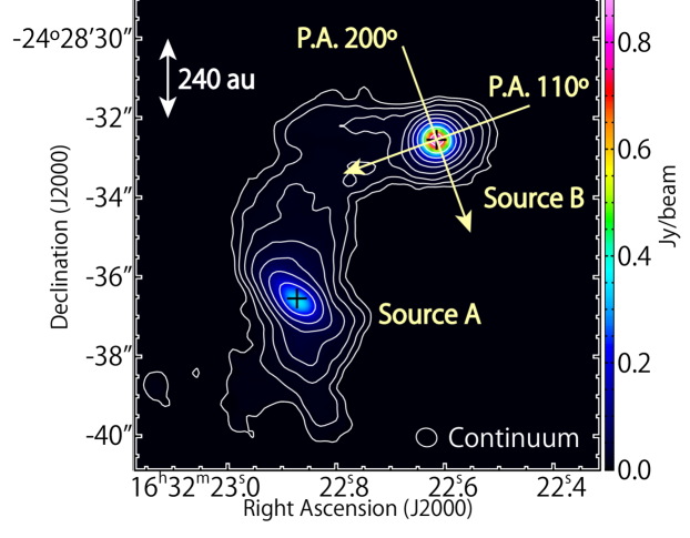
Figure 1: Map of the continuum emission at the 1.3 mm (236 GHz) band. The contour levels are 10, 20, 40, 80, 160, 320, 640, 1280, and 2560$\sigma$, where the rms noise level is 0.3 mJy beam^-1. The intensity peak positions are shown by the black crosses. The synthesized beam is depicted in the bottom-right corner. PA of 110° and 200° indicate the disk/envelope direction and the direction perpendicular to it.

Figure 1 shows the 1.3 mm (236 GHz) continuum map. The synthesized beam is $(0\farcs 524\times 0\farcs 463)$ (PA $73.\!\!\arcdeg 87$). There are two intensity peaks corresponding to the two components of the binary, Source A and Source B. A weak emission bridging between the two peaks can also be seen. These features are consistent with the previous report by Jørgensen et al. (2016). While the distribution around Source A is slightly elongated along the NE-SW direction, that around Source B has an almost round shape. The disk/envelope systems of Source A and B are reported to have nearly edge-on and face-on configurations, respectively (e.g. Rodríguez et al., 2005; Chandler et al., 2005), to which the above distributions are consistent. The full-width half-maximum (FWHM) sizes, the peak flux densities, and the peak position for Source A and Source B are determined by a two-dimensional Gaussian fit to the image. The FWHM sizes deconvolved by the beam are evaluated to be $(1\farcs 138\pm 0\farcs 007)\times(0\farcs 583\pm 0\farcs 004)$ (PA $36.\!\!\arcdeg 1\pm 0.\!\!\arcdeg 35$) and $(0\farcs 429\pm 0\farcs 003)\times(0\farcs 357\pm 0\farcs 003)$ (PA $139.\!\!\arcdeg 0\pm 1.\!\!\arcdeg 6$) for Source A and Source B, respectively. The peak flux densities are $(314.0\pm 1.4)$ and $(899.9\pm 1.5)$ mJy/beam for Source A and Source B, respectively. The derived continuum peak positions are: ($\alpha_{2000}$, $\delta_{2000}$) = ($16^{\rm h}32^{\rm m}22\fs 8725\pm 0\fs 0001$, $-24\arcdeg 28\arcmin 36\farcs 536\pm 0\farcs 002$) and ($\alpha_{2000}$, $\delta_{2000}$) = ($16^{\rm h}32^{\rm m}22\fs 61531\pm 0\fs 00003$, $-24\arcdeg 28\arcmin 32\farcs 5467\pm 0\farcs 0004$), for Source A and Source B, respectively. Although they may be affected by the self-calibration, the effect seems to be negligible for a beam size of $\sim 0\farcs 5$. Indeed, the continuum peak position of Source B was derived to be ($\alpha_{2000}$, $\delta_{2000}$) = ($16^{\rm h}32^{\rm m}22\fs 6142\pm 0\fs 0001$, $-24\arcdeg 28\arcmin 32\farcs 524\pm 0\farcs 002$) without self-calibration processing, and the difference from the position derived from the self-calibrated data is very small ($\sim 0\farcs 03$).

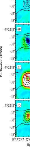
Figure 2: The velocity channel maps of the OCS ($J=19-18$) line. The $v_{\rm LSR}$ is shown in the left-upper corner of each panel, where the systemic velocity is $\sim 3$ km s^-1. The contours represent the continuum map (see Figure 1), whose intensity peak position is shown by the black crosses. The contour levels are 20, 80, 320, and 1280$\sigma$, where the rms noise level is 0.3 mJy beam^-1. The synthesized beams are depicted at the bottom.

Figure 2 shows the velocity channel maps of the OCS ($J=19-18$) line. Absorption toward the continuum peak position can be seen in the channels with $v_{\rm LSR}$ ranging from 3.4 to 4.3 km s^-1. Since the systemic velocity is around 3 km s^-1 (Bottinelli et al., 2004), this absorption feature is red-shifted. It is most naturally interpreted as the inverse P-Cygni profile, as previously reported by Jørgensen et al. (2012), Pineda et al. (2012), and Zapata et al. (2013). At the systemic velocity, the distribution is extended at a 3″ ($\sim$400 au) scale in diameter around the continuum peak, although it would suffer from the resolving-out effect with the largest recoverable scale of $\sim$14″ in this observation.

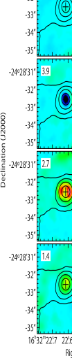
Figure 3: The velocity channel maps of the CH₃OH ($5_{1,5}-4_{1,4}$; A⁺) line. The $v_{\rm LSR}$ is shown in the left-upper corner of each panel, where the systemic velocity is $\sim 3$ km s^-1. The contours represent the continuum map (see Figure 1), whose intensity peak position is shown by the black crosses. The contour levels are the same as those in Figure 2. The synthesized beams are depicted at the bottom.

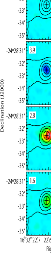
Figure 4: The velocity channel maps of the HCOOCH₃ ($20_{3,17}-19_{3,16}$; A) line. The $v_{\rm LSR}$ is shown in the left-upper corner of each panel, where the systemic velocity is $\sim 3$ km s^-1. The contours represent the continuum map (see Figure 1), whose intensity peak position is shown by the black crosses. The contour levels are the same as those in Figure 2. The synthesized beams are depicted at the bottom.

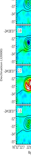
Figure 5: The velocity channel maps of the H₂CS ($7_{0,7}-6_{0,6}$) line. The $v_{\rm LSR}$ is shown in the left-upper corner of each panel, where the systemic velocity is $\sim 3$ km s^-1. The contours represent the continuum map (see Figure 1), whose intensity peak position is shown by the black crosses. The contour levels are the same as those in Figure 2. The synthesized beams are depicted at the bottom.

Figures 3, 4, and 5 show the velocity channel maps of the CH₃OH ($5_{1,5}-4_{1,4}$; A⁺), HCOOCH₃ ($20_{3,17}-19_{3,16}$; A), and H₂CS ($7_{0,7}-6_{0,6}$) lines, respectively. For all the three lines, the red-shifted components of the emission ($v_{\rm LSR}$ = 3–5 km s^-1) show absorption features toward the continuum peak as in the OCS case. The distributions of CH₃OH and HCOOCH₃ are more compact than that of OCS. Although the distribution of H₂CS is also smaller than that of OCS around the protostar, it is larger than those of CH₃OH and HCOOCH₃. The H₂CS emission is slightly extended toward the western side of the continuum peak.

The integrated intensity maps of the four molecular species are shown in Figure 6. The intensity distributions, except for that of HCOOCH₃, show a ring-like structure around the protostar; the molecular line intensities are weaker within a radius of 0$\farcs$25 ($\sim$30 au) toward the continuum peak position than the surrounding positions. This is due to the contribution of the inverse P-Cygni profile toward the continuum peak position, as shown in the channel maps (Figures 2, 3, and 5).

The different sizes of the molecular distributions seen in the channel maps can also be confirmed in the integrated intensity maps. Indeed, the OCS distribution is clearly extended over 1″ ($\sim$120 au) around the protostar. The CH₃OH and HCOOCH₃ emission is concentrated around the protostar with a radius of 0$\farcs$6 ($\sim$70 au). It should be noted that a weak emission of CH₃OH is seen at the angular distance of 2″ and 3″ in the northern and southern sides of the protostar, respectively. Although their origin is puzzling, these components may be related to the outflow originating from Source B (see Section 4), or may be enhanced by an interaction between the envelope gas and the outflow from Source A, as suggested from the CO ($J=6-5$) observations (Kristensen et al., 2013). Probably, extended components of the outflows would be resolved out in the present study. The H₂CS ($7_{0,7}-6_{0,6}$) emission is slightly more extended than the CH₃OH and HCOOCH₃ emission, but is not so extended as the OCS emission. The distributions of the higher excitation lines of H₂CS ($7_{2,5}-6_{2,4}$; $7_{4}-6_{4}$) tend to be as compact as those of the CH₃OH and HCOOCH₃ lines.

3.2 Chemical Differentiation

The above results for OCS, CH₃OH, HCOOCH₃, and H₂CS show small-scale chemical differentiation in the vicinity of the protostar in Source B. This differentiation is clearly confirmed by the spatial profiles of the integrated line intensities of these molecules, as shown in Figure 7. Only the blue-shifted components, which are in the velocity range from 0.9 to 2.9 km s^-1, are integrated to prevent contamination of the inverse P-Cygni profile. The position axis of the spatial profiles has the origin at the continuum peak, and is prepared along the line where the disk/envelope system is extended. Its position angle is 110°, as described in Section 4.1 (Figures 1 and 8).

In IRAS 16293–2422 Source B, it is well-known that the molecular line emission associated with the main molecular isotopologues is often optically thick (e.g., Jørgensen et al., 2016). In such a case, the line intensities do not reflect their actual abundances, especially toward the continuum peak. Thus, we need to consider the optical depth effect carefully. However, we confirm by a non-LTE excitation calculation that the optical depth effect does not affect the difference of the emitting regions shown in Figure 7. Here, we used the RADEX code (van der Tak et al., 2007) assuming a kinetic temperature of 100 K and a $n$(H₂) of $10^{8}$ cm^-3. In this calculation, the optical depths of the OCS and CH₃OH lines are roughly estimated to be about 0.2 and 0.01, respectively, at the angular offset of $-1$″ (corresponding to $-120$ au) from the continuum peak in Figure 7, where their integrated intensities are 0.45 and 0.03 Jy beam^-1 km s^-1, respectively. The excitation temperatures are 100 and 97 K for the OCS and CH₃OH lines, respectively, indicating that the lines are well thermalized.

Since the excitation temperatures employed by Coutens et al. (2016) are between 100 and 300 K at 0$\farcs$5 from the protostar, the kinetic temperature would be higher than 70 K at 1$\farcs$0. Even in this condition, the optical depths of OCS and CH₃OH are estimated to be lower than 0.3 according to the RADEX code. It should be noted that the above results for the optical depths do not change significantly for a $n$(H₂) from $10^{6}$ to $10^{9}$ cm^-3.

Thus, the gradual change in the OCS intensity and the CH₃OH intensity can be attributed to the difference in their respective distributions. In addition, the excitation effect cannot make the OCS distribution more extended in comparison with that of CH₃OH and HCOOCH₃, because the upper-state energy for the OCS line is comparable to that of the HCOOCH₃ line and is even higher than those of the CH₃OH and H₂CS lines (Table 1). Thus, the different distributions seem to mainly represent the change in the chemical composition of the gas.

A similar chemical differentiation is also seen in Source A; the distributions of CH₃OH and HCOOCH₃ are concentrated around the centrifugal barrier with the radius of 50 au, while the OCS and H₂CS distributions are more extended (Oya et al., 2016). In that context, Miura et al. (2017) recently reported on the basis of numerical simulations that the enhancement of the COM lines around the centrifugal barrier can be caused by the dust heating in accretion shocks in front of the centrifugal barrier.

4 Kinematic Structure

4.1 Rotation Feature

The velocity widths (FWHM) of these line emissions toward Source B are as narrow as 3 km s^-1. They are narrower than those toward Source A, which are typically wider than 5 km s^-1. The narrow velocity widths likely originate from the nearly face-on geometry of the disk/envelope system of Source B, as mentioned in Section 1. Nevertheless, we can recognize small velocity gradient in the channel maps of OCS (Figure 2). This result indicates that the disk/envelope system is slightly inclined. At the blue-shifted velocity ($v_{\rm LSR}$ $\sim$1.5 km s^-1), the OCS distribution shows a slight offset from the continuum peak position toward the northwestern (NW) direction, while at the red-shifted velocity ($v_{\rm LSR}$ $\sim$4 km s^-1), it tends to have a slight offset toward the southeastern (SE) direction. This trend can be confirmed in the integrated intensity maps of the high velocity-shifted components (Figure 8); although the red-shifted component may be contaminated by the absorption toward the continuum peak, the blue-shifted component of the OCS line seems to be aligned on a straight line along the SE-NW direction with a position angle (PA) of about 110°. This velocity gradient suggests a rotation motion of the disk/envelope system, slightly inclined from the face-on geometry. In the below analysis, we use the position angle of 110° as the direction along which the mid-plane of the disk/envelope system is extended (hereafter ‘the disk/envelope direction’).

4.2 Observed Features

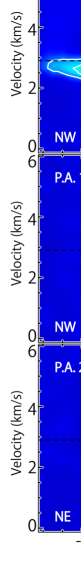
Figure 9: The position-velocity diagrams of the OCS ($J=19-18$) line. The position axes are centered at the continuum peak position and their position angles are every 30° from 110°. The contour levels are from $-40\sigma$ and every 20$\sigma$, except for 0$\sigma$, where the rms noise level is 3.2 mJy beam^-1. The rectangle in each panel represents the spatial and velocity resolutions.

Figures 9 to 12 show the position-velocity (PV) diagrams of OCS, H₂CS, CH₃OH, and HCOOCH₃ that allow us to investigate the velocity structure around the protostar. In the PV diagrams, the inverse P-Cygni profile is confirmed toward the protostar. Along the PA of 110°, a slight velocity gradient can be seen in the OCS line (Figure 9), although it is heavily contaminated with the absorption feature toward the continuum peak position. The velocity in the northwestern side tends to be lower than that in the southeastern side. In this diagram, the position of the intensity peak has a slight offset from the continuum peak position. The PV diagrams along the lines with various PAs also show the absorption feature toward the continuum peak position. Moreover, the PV diagrams along the lines with the PAs of 140°, 170°, 200°, and 230° show two intensity peaks with an offset from the continuum peak position. For instance, the peak intensity ($\sim$0.6 Jy beam^-1) is about 1.5 times higher than the intensity toward the continuum peak position ($\sim$0.4 Jy beam^-1) in the PV diagram along the line with the PA of 200°.

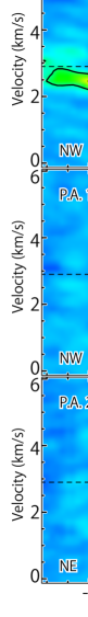
Figure 10: The position-velocity diagrams of the H₂CS ($7_{0,7}-6_{0,6}$) line. The position axes are the same as those in Figure 9. The contour levels are from -20$\sigma$ and every 10$\sigma$, except for 0$\sigma$, where the rms noise level is 2.3 mJy beam^-1. There is a contamination by another molecular line with a velocity offset of 2 km s^-1. The rectangle in each panel represents the spatial and velocity resolutions.

The PV diagram of the H₂CS ($7_{0,7}-6_{0,6}$) line along the PA of 110° shows a slight velocity gradient similar to the OCS case (Figure 10). The absorption in the red-shifted component toward the continuum peak can be confirmed. There is another absorption feature with the velocity higher than 5 km s^-1, which is likely to be a contamination by an unidentified line. As in the case of OCS, the H₂CS line also shows two intensity peaks in the PV diagrams except for that along the PA of 200° (i.e. the direction perpendicular to the disk/envelope direction). The intensity dip toward the continuum peak position is clearer in H₂CS than in OCS. In fact, the peak integrated intensity ($\sim$0.57 Jy beam^-1 km s^-1) is twice higher than the intensity toward the continuum peak (0.45 Jy beam^-1 km s^-1) in Figure 7. The peak intensities have asymmetry in the PV diagrams; the peak intensity at the southern side of the protostar is higher than at the northern side, except for the PV diagram along the PA of 110°. This may be caused by the asymmetric distribution of the gas.

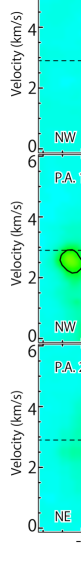
Figure 11: The position-velocity diagrams of the CH₃OH ($5_{1,5}-4_{1,4}$; A⁺) line. The position axes are the same as those in Figure 9. The contour levels are from -100$\sigma$ and every 20$\sigma$, except for 0$\sigma$, where the rms noise level is 2.5 mJy beam^-1. The rectangle in each panel represents the spatial and velocity resolutions.

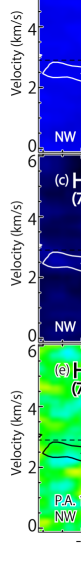
Figure 12: The position-velocity diagrams of the HCOOCH₃ ($20_{3,17}-19_{3,16}$; A) and two H₂CS ($7_{2,5}-6_{2,4}$; $7_{4}-6_{4}$) lines. The position axes are the same as those in the panels of P.As. of 110° and 200° in Figure 9. The contours in each panel represent the PV diagram of H₂CS ($7_{0,7}-6_{0,6}$), which are as the same as those in Figure 10. The rectangle in each panel represents the spatial and velocity resolutions.

On the other hand, the PV diagrams of the CH₃OH and HCOOCH₃ lines do not show such a clear velocity gradient, as shown in Figures 11 and 12(a, b), respectively. The absence of the apparent velocity gradient for these lines seems to originate from the contamination of the inverse P-Cygni profile. The distributions of the CH₃OH and HCOOCH₃ emission along the PA of 110° is as compact as 1$\farcs$5. Their maximum velocity shift from the systemic velocity ($\sim 3$ km s^-1) is 2 km s^-1, which is comparable to that for OCS. The distributions for the CH₃OH and HCOOCH₃ lines are so compact that the red-shifted part of their emission near the continuum peak is heavily obscured by the unresolved absorption feature of the inverse P-Cygni profile. We also prepare the moment 1 maps (not shown in this article) of the CH₃OH and HCOOCH₃ lines to closely inspect the velocity gradient in these lines. However, no significant features of the velocity gradient can be seen for these lines. It should be noted that the compact distributions of the CH₃OH and HCOOCH₃ emission are not due to excitation effect, because the upper-state energies of these lines are comparable to or even lower than that of OCS (See Table 1).

In Figure 11, all the six PV diagrams of CH₃OH show some asymmetry with respect to the continuum peak position. They are essentially similar to one another in the sizes of the absorption and the emission. This asymmetry in the intensities seems to be anti-correlated to that seen in the H₂CS line for the PV diagrams along the PA of (140–200)°. Although the reason of this anticorrelation is puzzling at present, such a chemical differentiation could be a key to understand chemical processes occurring there.

4.3 Comparison of the Observed Molecular Distributions with the Source A Case

Since rotation motion around Source B is suggested by the OCS and H₂CS emission, we investigate its kinematic structure in more detail. As for Source A, we successfully explained the kinematic structure of the infalling-rotating envelope at a 100 au scale by a ballistic model (Oya et al., 2014, 2016). Hence, we take the advantage of this knowledge in the analysis of the Source B data.

In Source A, OCS traces the infalling-rotating envelope, while the COMs highlight the centrifugal barrier, as mentioned in Section 1. This situation is consistent with the chemical differentiation in Source B, where the OCS distribution is rather extended while the CH₃OH and HCOOCH₃ distributions are compact around the protostar. If the OCS line traces the infalling-rotating envelope, the velocity gradient shown in Figure 9 can be interpreted by a combination of the infall and rotation motions in the envelope. The size of the CH₃OH and HCOOCH₃ emission would be close to the size of the centrifugal barrier, as in the case of Source A. These features will be examined by our kinematic model in Section 5.

On the other hand, the distribution of H₂CS in Source B inside the centrifugal barrier seems different from that in Source A. In Source A, high velocity-shift components tracing the disk component inside the centrifugal barrier are observed. In contrast, such components are not apparently seen in Source B. The PV diagram shows a double-peaked structure having an intensity dip at the continuum peak position (Figure 10). This dip structure does not originate from the high dust opacity, because the emission, particularly at the blue-shifted one, is indeed observed toward the continuum peak position in other molecular lines: the PV diagrams of the CH₃OH, HCOOCH₃, and H₂CS ($7_{2,5}-6_{2,4}$; $7_{4}-6_{4}$) lines show a compact emission in Figures 11 and 12. The dip is not due to the absorption by the foreground gas either, because the dip is seen at the velocity shift of $-1$ km s^-1 from the systemic velocity ($\sim 3$ km s^-1). Hence, the intensity dip means that H₂CS would be deficient in the closest vicinity of the protostar. The two intensity peaks in the PV diagram just correspond to the position within which CH₃OH and HCOOCH₃ appear (Figures 12a, b). Although the double-peaked structure is not clearly seen in OCS (Figure 9), the intensity peak of OCS seems to be shifted from the continuum peak position and almost coincides one of the intensity peaks of H₂CS. Considering that CH₃OH and HCOOCH₃ are concentrated around the centrifugal barrier in Source A, it is most likely that the two intensity peaks in the PV diagram of H₂CS represent the positions of the centrifugal barrier in Source B.

Figure 13(a) shows a schematic illustration of the above configuration of the disk/envelope system. The structure of the outflow is consistent with the configuration, as described later (Section 6).

5 Modelling

5.1 Infalling-Rotating Envelope Model

We investigate the velocity gradient observed in the OCS ($J=19-18$) and H₂CS ($7_{0,7}-6_{0,6}$) lines, using the infalling-rotating envelope model by Oya et al. (2014). Since the velocity gradient is seen as the double-peaked structure in the PV diagram of H₂CS ($7_{0,7}-6_{0,6}$) along the disk/envelope direction (PA 110°), as mentioned above, we evaluate the physical parameters by comparing the model with this PV diagram.

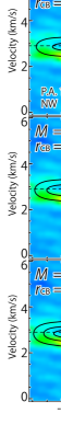
Figure 14: The position-velocity diagrams of the H₂CS ($7_{0,7}-6_{0,6}$; color) along the disk/envelope direction (PA 110°), where the color maps are the same as the panel of a PA 110° in Figure 10. The black contours represent the results of infalling-rotating envelope models. The physical parameters for the models are: $M$ = 0.2, 0.4, and 0.8 $M_{\odot}$; $r_{\rm CB}$ = 20, 40, and 60 au; and $i$ = 5°. The contour levels are every 20% from 5% of each peak intensity. The rectangle in the top left panel represents the spatial and velocity resolutions.

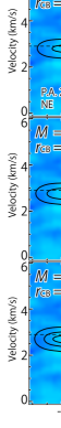
Figure 15: The position-velocity diagrams of the H₂CS ($7_{0,7}-6_{0,6}$; color) line along the line perpendicular to the disk/envelope direction (PA 200°), where the color maps are the same as the panel of a PA 200° in Figure 10. The black contours represent the results of infalling-rotating envelope models. The physical parameters for the models are: $M$ = 0.2, 0.4, and 0.8 $M_{\odot}$; $r_{\rm CB}$ = 20, 40, and 60 au; and $i$ = 5°. The contour levels are every 20% from 5% of each peak intensity. The rectangle in the top left panel represents the spatial and velocity resolutions.

Figures 14 and 15 show examples of the infalling-rotating envelope models superposed on the PV diagram of the H₂CS ($7_{0,7}-6_{0,6}$) line along the disk/envelope direction and the direction perpendicular to it, respectively. We here adopt the systemic velocity of 2.9 km s^-1 in the model. In the infalling-rotating envelope model, the main physical parameters are the protostellar mass ($M$) and the radius of the centrifugal barrier ($r_{\rm CB}$). To see how the PV diagrams of the infalling-rotating envelope model depend on these parameters, we conduct the simulations for various sets of the parameters. We assume an envelope with a constant thickness of 50 au and the outer radius of 300 au with the inclination angle of 5° (0° for a face-on configuration). We also assume the intrinsic line width of 0.5 km s^-1. The model image is convolved with the synthesized beam. Since we are interested in the kinematic structure around the protostar, the emissivity is simply assumed to be proportional to the H₂ density ($n$(H₂) $\propto r^{-1.5}$) in the infalling-rotating envelope, and no radiative transfer effect is considered in this model. Namely, we do not make fine tuning of the intensity distribution, but we rather just focus on the fundamental characteristics of the kinematic structure. Since the red-shifted components in these observations suffer from the absorption feature of the inverse P-Cygni profile, we mainly consider the kinematic structure of the blue-shifted components.

As shown in Figure 14, the velocity gradient along the disk/envelope direction seems to be reasonably explained by the rotating motion in the infalling-rotating envelope model. Especially, the models with $r_{\rm CB}$ of 40 au well reproduce the observations except for the absorption feature. Although the model depends on the protostellar mass ($M$), it is not well constrained due to the contamination of the absorption feature. Hence, it is estimated to be around 0.4 $M_{\odot}$ within a factor of 2 assuming the inclination angle of the disk/envelope system of 5°. On the other hand, the model result strongly depends on $r_{\rm CB}$. In the models with $r_{\rm CB}$ of 60 au, the distance between the two intensity peaks is larger than that observed, because the positions of the two peaks in the model correspond to those of the centrifugal barrier. In the models with $r_{\rm CB}$ of 20 au, the emission seems to be concentrated toward the protostar. This is because the emission at the centrifugal barrier is not resolved with the synthesized beam in the model, and thus the observed double-peaked structure cannot be reproduced. Hence, $r_{\rm CB}$ is evaluated to be $(30-50)$ au. In the PV diagram along the line perpendicular to the disk/envelope direction (PA 200°; Figure 15), the models with $r_{\rm CB}$ of 40 au show a better agreement with the observations than those with $r_{\rm CB}$ of 20 or 60 au, although the observations show an asymmetric distribution of the emission.

The inclination angle of 5° is fixed in the above analysis, where the northeastern side of the disk/envelope system faces to us. The velocity gradient cannot be explained with the inclination angle of 0° (completely face-on configuration) or a negative value, where the southwestern side of the disk/envelope system faces to us. Likewise, the velocity structure cannot be reproduced either with the inclination angle larger than 15°.

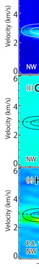
Figure 16: The position-velocity diagrams of the OCS ($J=19-18$; a, b), CH₃OH ($5_{1,5}-4_{1,4}$; A⁺; c, d), and H₂CS ($7_{0,7}-6_{0,6}$; e, f) lines along the disk/envelope direction (PA 110°) and the direction perpendicular to it (PA 200°), where the color maps are the same as the panels (a, d) in Figures 9–10. The black and white contours represent the results of the infalling-rotating envelope model, where the physical parameters are $M$ = 0.4 $M_{\odot}$, $r_{\rm CB}$ = 40 au, and $i$ = 5°. The contour levels are every 20% from 5% of each peak intensity. The rectangle in each panel represents the spatial and velocity resolutions.

The comparison between the infalling-rotating envelope model and the OCS ($J=19-18$) and CH₃OH ($5_{1,5}-4_{1,4}$; A⁺) lines are also shown in Figure 16. Here the model with $M$ of 0.4 $M_{\odot}$ and $r_{\rm CB}$ of 40 au is employed as a representative set of the parameters. Strictly speaking, the OCS ($J=19-18$) line does not show a clear double-peaked feature unlike the H₂CS ($7_{0,7}-6_{0,6}$) line. Nevertheless, the model seems to explain the basic velocity feature of the PV diagram of the OCS ($J=19-18$) line, except for the absorption feature. On the other hand, the kinematic structure traced by the CH₃OH ($5_{1,5}-4_{1,4}$; A⁺) line cannot be explained by the infalling-rotating envelope model obtained from the above analysis. The emitting region of the CH₃OH ($5_{1,5}-4_{1,4}$; A⁺) line seems to be concentrated around the centrifugal barrier and/or inside it. This is consistent with the Source A case, where the CH₃OH (11${}_{0,11}-10_{1,10}$; A⁺) line mainly highlights the centrifugal barrier and/or inside it (Oya et al., 2016).

5.2 Origin of the inverse P-Cygni Profile

Although the basic feature of the kinematic structure traced by the OCS and H₂CS lines is reasonably explained by the infalling-rotating envelope model (Figure 16) as discussed above, there remains an important problem: how can we interpret the inverse P-Cygni profile? The inverse P-Cygni profile means an infall motion along the line of sight toward the protostar. Since the disk/envelope system is nearly face-on, the outflow motion would also exist along the line of sight, as shown in Section 6. This situation, namely the coexistence of the infall motion and the outflow motion along the line-of-sight in the vicinity of the protostar, is hardly possible, as far as we consider the thin disk structure such as Figure 13(a). At least, a thick disk/envelope structure would be necessary so as that substantial amount of the infalling gas exists near the protostar. In fact, such an infall component perpendicular to the mid-plane near the launching point of the outflow is seen in numerical simulations of outflows (Machida & Hosokawa, 2013). Even in this case, there remains the following difficulty. Since the velocity shift of the absorption feature from the systemic velocity ($\sim 3$ km s^-1) is at most 2 km s^-1 (Figure 11), the infalling gas at this velocity-shift has to be located at 180 au, assuming the free-fall with the protostellar mass of 0.4 $M_{\odot}$. This distance is much larger than the apparent size of the COM emission ($\sim$50 au) around the protostar, which accompanies the inverse P-Cygni profile.

Recently, a hint to solve this problem is found in the other protostellar source L1527. On the basis of the high-resolution molecular line observations with ALMA, Sakai et al. (2017) reported that the thickness of the disk/envelope system is broadened at the centrifugal barrier and inward of it due to the stagnation of the accreting gas. A part of the stagnant gas at the centrifugal barrier once moves toward the out-of-plane direction, and falls toward the protostar, if its angular momentum is extracted by some mechanisms (i.e. disk winds and/or low-velocity outflows (c.f., Alves et al., 2017)). If this situation is also the case for Source B, such an infalling gas may cause the inverse P-Cygni profile. This situation is schematically illustrated in Figure 13(b).

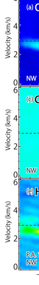
Figure 17: The position-velocity diagrams of the OCS ($J=19-18$; a, b), CH₃OH ($5_{1,5}-4_{1,4}$; A⁺; c, d), and H₂CS ($7_{0,7}-6_{0,6}$; e, f) lines along the disk/envelope direction (PA 110°) and the direction perpendicular to it (PA 200°), where the color maps are the same as those in Figures 16. The black and white contours represent the results of the model for the infall motion from the centrifugal barrier. The physical parameters are $M$ = 0.4 $M_{\odot}$, $r_{\rm CB}$ = 40 au, and $i$ = 5°. The molecular line emission is assumed to be in the region with the distance from the protostar of (35–40) au. The contour levels are every 20% from 5% of each peak intensity. The rectangle in each panel represents the spatial and velocity resolutions.

Hence, we incorporate the free-fall motion in the vicinity of the protostar in the model. We approximate the gas distribution around the protostar as a spherical clump with a radius of the centrifugal barrier for simplicity. This model simulates the hypothetical situation that the infalling gas is once stagnated at the distance of 40 au ($r_{\rm CB}$) from the protostar to make a spherical clump, and then it falls to the protostar by the gravity without the initial radial speed. Here, the ‘spherical clump’ mimics the gas stagnation, although the gas distribution is not spherical in reality. Figure 17 shows the results. This very simplified picture can explain the kinematic structure of CH₃OH at a 40 au scale around the protostar, including the velocity of the absorption in the inverse P-Cygni profile. The kinematic structures of OCS and H₂CS, on the other hand, seem to be explained by the combination of the infalling-rotating envelope model for the extended components and this free-fall picture for the inverse P-Cygni profile. In this free-fall picture, the absorption gas for the inverse P-Cygni profile having the infall velocity of 2 km s^-1 is located at 33 au from the protostar, which is smaller than the size of their apparent distribution. However, it should be stressed that this model is just a simplified one representing the above hypothetical physical picture. We need to resolve the structure of the vicinity of the protostar to verify its validity.

6 Outflow

We have also analyzed the SiO ($J=6-5$) data. Figure 18 shows the integrated intensity maps of the high velocity-shift components traced by SiO. This molecule is often employed as a shock tracer (e.g., Mikami et al., 1992; Bachiller & Pérez Gutiérrez, 1997). Both the blue-shifted and red-shifted components show a shell-like feature surrounding the continuum peak, which are spatially overlapped with each other even at a 300 au scale. Kristensen et al. (2013) have suggested by using the CO ($J=6-5$) ALMA observation that there is an interaction of the outflow from Source A with Source B, resulting in shocks there. In addition, Girart et al. (2014) have also detected the SiO ($J=8-7$) line around Source B, and have suggested that the SiO morphology is consistent with an interaction of the outflow from Source A with Source B. Nevertheless, the authors did not investigate the kinematics. Although this possibility cannot be ruled out, these SiO components can also be attributed to the outflow from Source B with a nearly pole-on geometry; namely, its kinematic structure is consistent with the situation that we are looking at the outflow cavities as a shell-like feature. We favor this possibility, because the CO outflow from Source A is blue-shifted while the SiO emission has the red-shift component. Moreover, the interaction cannot be seen clearly in the other lines. For instance, no enhancement of CH₃OH is seen in the southeastern side (Figure 16c). Furthermore, the SiO emission can be seen in the back side of Source B with respect to the direction to Source A.

When we look at the two components of SiO closely (Figure 18), the blue-shifted components are slightly extended toward the northeastern direction from the continuum peak. On the other hand, the red-shifted emission is stronger than the blue-shifted one in the southwestern side of the continuum peak. Hence, the outflow axis might be inclined slightly (positive inclination angle), as illustrated in Figure 13. Thus, the blue-shifted outflow lobe seems to be overlapped on the protostar along the line of sight. This interpretation is natural, because the disk/envelope system has a face-on geometry. The positive inclination angle is consistent with that suggested by the analysis of the disk/envelope system.

In the OCS, CH₃OH, HCOOCH₃, and H₂CS lines, the inverse P-Cygni profile is seen toward the protostar. As discussed in Section 5.2, the picture shown in Figure 13(b) allows the coexistence of the blue-shifted outflow lobe and the infalling gas toward the protostar. In this case, the outflow responsible for the above SiO distribution would be not launched directly from the protostar, but could be from the inner part of the disk/envelope system possibly around the centrifugal barrier. In fact, there is a hint for such a situation in the kinematic structure of the SiO emission. The SiO emission shows the bipolar outflow lobes along the PA of 200°, as shown in Figure 19. In this figure, we note that there are the two absorption features toward the continuum peak position, which are likely due to the contamination by other molecular lines with the inverse P-Cygni profile. The blue-shifted and red-shifted lobes are seen in both the northeastern and southwestern sides of the continuum peak, which is consistent with the configuration shown in Figure 13(b). If the outflow is accelerated as it propagates away from the protostar (e.g. Lee et al., 2000), the systemic velocity ($\sim 3$ km s^-1) component may approximately regarded as the outflow component at its launching point. At the systemic velocity, the SiO emission is seen at the position with an offset of $\sim$0$\farcs$5 from the continuum peak, but not toward the protostar. The radial size of the SiO dip is larger than those of the OCS and H₂CS emission in Figure 19. Hence, this feature is not likely to be due to the optical depth effect toward the continuum peak. This implies that the launching point of the outflow has a radial offset from the protostar (Figure 13b). Moreover, the SiO emission at the systemic velocity seems to appear near to the intensity peak of the OCS and H₂CS emission. This feature may suggest that the launching point of the outflow could be around the centrifugal barrier traced by OCS and H₂CS. A similar situation is recently reported for BHB07-11 (Alves et al., 2017).

Large-scale outflows blowing out from this binary system have extensively been studied (e.g. Mizuno et al., 1990; Hirano et al., 2001). Their directions are different from that found in this study. This contradiction may be due to the complexity of the binary system. The dynamical timescale of the outflow lobes at a larger scale $(10^{4}-10^{5})$ au is estimated to be $(10^{4}-10^{5})$ years (Mizuno et al., 1990; Hirano et al., 2001). On the other hand, it is reported that Source A and Source B are rotating around each other with the period of $\sim 2\times 10^{4}$ years (Bottinelli et al., 2004). Thus the directions of the two outflow can be modulated in a complex way. Hence, the small-scale outflow structure in the vicinity of a protostar has to be studied in order to explore the relation between the outflow and the disk/envelope system.

It should be noted that a small-scale outflow structure of IRAS 16293–2422 is investigated by using the CO lines with ALMA (Kristensen et al., 2013; Loinard et al., 2013; Girart et al., 2014). However, the outflow morphology seen in the CO lines in this source is very complicated. The northwest-southeast outflow is seen in Source A, while the outflow from Source B is unclear in these observations. In contrast, our kinematic analysis suggests a possibility that the SiO emission traces the outflow launched from Source B.

7 Gas Kinetic Temperature

For Source A, Oya et al. (2016) evaluated the gas kinetic temperature from the intensities of the two lines ($7_{0,7}-6_{0,6}$; $7_{2,5}-6_{2,4}$) of H₂CS. The lines of H₂CS with different $K_{\rm a}$ can be used as a good tracer of the gas kinetic temperature. As a result, it is found that the gas kinetic temperature around Source A once rises from the infalling-rotating envelope to the centrifugal barrier, and then drops in the disk component inside the centrifugal barrier.

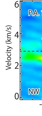
Figure 20: The position-velocity diagram of the H₂CS ($7_{0,7}-6_{0,6}$) line along the disk/envelope direction (PA 110°). The vertical edges of the black rectangles represent the velocity ranges which are integrated to derive the gas kinetic temperature in Section 7. The horizontal edges of them are centered at the positions at the distance of 0, $\pm$60, and $\pm$120 au from the continuum peak position along the disk/envelope direction (PA 110°), where the gas kinetic temperature is derived. The lengths of the horizontal edges of them correspond to the angular resolution for the H₂CS ($7_{0,7}-6_{0,6}$) line. The rectangle represents the spatial and velocity resolutions.

Here, we also evaluate the gas kinetic temperature around Source B from the H₂CS line intensities. Figures 12(c–f) show the PV diagrams of the high excitation lines of H₂CS ($7_{2,5}-6_{2,4}$; $7_{4}-6_{4}$) on which those of the H₂CS line ($7_{0,7}-6_{0,6}$) is superposed. The distributions of the higher excitation lines of H₂CS seem to be more concentrated to the continuum peak position than the H₂CS line ($7_{0,7}-6_{0,6}$). Thus the intensity ratio of a higher excitation line relative to the lower excitation line becomes higher toward the protostar. This implies that the gas kinetic temperature is raised as approaching to the continuum peak position. The gas kinetic temperature is evaluated by using the non-LTE code RADEX (van der Tak et al., 2007), as shown in Table 2. Temperatures are calculated for the positions with the radii of 0, 60, and 120 au from the continuum peak along the disk/envelope direction (PA 110°). For this calculation, we prepare the integrated intensity maps of the three H₂CS lines ($7_{0,7}-6_{0,6}$; $7_{2,5}-6_{2,4}$; $7_{4}-6_{4}$) with the velocity width of 1 km s^-1. The velocity-shift range from $-1.5$ to $-0.5$ km s^-1 is taken at the continuum peak position in order to extract the high velocity-shift component excluding the absorption effect. The H₂CS ($7_{4}-6_{4}$) line emission is detected with this velocity range (Figure 12). On the other hand, the velocity-shift range from $-0.5$ to $+0.5$ km s^-1 is taken for the positions at the distance of 60 and 120 au from the continuum peak position. The above velocity-ranges and the positions are shown in the PV diagram of H₂CS ($7_{0,7}-6_{0,6}$) (Figure 20). It should be noted that the H₂CS ($7_{0,7}-6_{0,6}$) line may possibly be optically thick toward the continuum peak. Hence, the intensity of the H₂CS ($7_{0,7}-6_{0,6}$) line may be attenuated, which would overestimate the gas kinetic temperature. Thus the values derived from the $7_{2,5}-6_{2,4}$ and $7_{4}-6_{4}$ lines (the second row in Table 2) may be more reliable than those derived from the $7_{0,7}-6_{0,6}$ and $7_{2,5}-6_{2,4}$ lines (the first row). The gas kinetic temperature is as high as $\sim$100 K within the radius of 60 au. Moreover, the temperature tends to be higher as getting close to the protostar probably due to the thermal heating by the protostar. In Source B, we do not find any particular enhancement of the gas kinetic temperature at the centrifugal barrier in contrast to the Source A case, probably because of the limited resolution of the observations. Higher angular resolution observations are required for further investigation on the small-scale temperature structure of this source.

8 Summary

We analyzed the OCS, CH₃OH, HCOOCH₃, H₂CS, and SiO data observed toward IRAS 16293–2422 Source B at a sub-arcsecond resolution with ALMA. Major findings are as follows:

(1) The chemical differentiation observed for the above molecules is similar to that found in Source A; OCS and H₂CS have more extended distributions than CH₃OH and HCOOCH₃.

(2) Although the disk/envelope system of Source B has a nearly face-on configuration, a modest rotation feature is implied in the extended component of the H₂CS and OCS lines. It is reasonably interpreted in terms of the infalling-rotating envelope model assuming the ballistic motion. On the other hand, the CH₃OH and HCOOCH₃ lines do not show a rotation feature. It might be due to the serious contamination of the unresolved absorption feature of the inverse P-Cygni profile.

(3) The bipolar outflow lobes near the protostar are likely detected in the SiO emission, although a possibility of the impact of the Source A outflow on Source B cannot be ruled out as the origin of the SiO emission. The blue and red lobes are largely overlapped, and hence, this feature is consistent with a nearly pole-on geometry of the disk/envelope system of this source.

(4) The molecular lines, except for HCOOCH₃, show absorption features toward the protostar. It is interpreted as the inverse P-Cygni profile by the infalling gas along the line of sight, as previously reported. The infall motion is reasonably explained by the free-fall motion of the gas stagnated around the centrifugal barrier, although it is a tentative and quite simplified interpretation.

(5) The coexistence of the outflow and the infall motion toward the protostar may suggest that the current launching point of the outflow responsible for the SiO emission likely has an offset from the protostar.

(6) The gas kinetic temperature is evaluated by using the H₂CS lines. The gas kinetic temperature is found to be as high as $\sim$100 K, which is consistent to the hot corino character of IRAS 16293–2422 Source B. The temperature is systematically higher toward the continuum peak position than toward the outer positions. No enhancement of the temperature is seen around the centrifugal barrier in contrast to the Source A case.

Table 1: Parameters of the Observed Lines

Molecule	Transition	Frequency (GHz)	$E_{\rm u}$ (K)	$S\mu^{2}$ (Debye2)	Synthesized Beam
OCS	$J=19-18$	231.0609934	111	9.72	$0\farcs 65\times 0\farcs 52$ (PA 84.​​°49)
CH3OH	$5_{1,5}-4_{1,4}$; A+	239.746253	49	3.89	$0\farcs 53\times 0\farcs 46$ (PA 71.​​°45)
HCOOCH3	$20_{3,17}-19_{3,16}$; A	250.25837	134	51.1	$0\farcs 61\times 0\farcs 46$ (PA 79.​​°40)
H2CS	$7_{0,7}-6_{0,6}$	240.2668724	46	19.0	$0\farcs 53\times 0\farcs 46$ (PA 73.​​°50)
H2CS	$7_{2,5}-6_{2,4}$	240.5490662	99	17.5	$0\farcs 53\times 0\farcs 46$ (PA 73.​​°67)
H2CS	$7_{4,4}-6_{4,3}$, $7_{4,3}-6_{4,2}$	240.3321897	257	12.8, 12.8	$0\farcs 53\times 0\farcs 46$ (PA 73.​​°58)
SiO	$J=6-5$	260.5180090	43.8	57.6	$0\farcs 74\times 0\farcs 59$ (PA 89.​​°09)

Table 2: Gas Kinetic Temperature Derived from the H₂CS Lines

	Offset from the protostar
Transitions	$-$120	$-$60	0 au	$+$60	$+$120
$7_{2,5}-6_{2,4}$ / $7_{0,7}-6_{0,6}$	$55-96$	$>338$	$>400$	$90-115$	$48-167$
$7_{4}-6_{4}$/ $7_{2,5}-6_{2,4}$	$>113$	$67-103$	$88-164$	$70-125$	$-$

Figure 6: The integrated intensity maps of the OCS ($J=19-18$), CH₃OH ($5_{1,5}-4_{1,4}$; A⁺), HCOOCH₃ ($20_{3,17}-19_{3,16}$; A), and H₂CS ($7_{0,7}-6_{0,6}$; $7_{2,5}-6_{2,4}$; $7_{4}-6_{4}$) lines associated with Source B (color). The contours represent the continuum map, where the contour levels are the same as those in Figure 1. The continuum peak positions are shown by the black crosses. The synthesized beam are depicted in the top-left corners.

Figure 7: The spatial profile of the integrated intensities of the observed molecular lines, where the integrated velocity range is from 0.9 to 2.9 km s^-1 ($v_{\rm sys}$ = 2.9 km s^-1). The position axis is centered at the continuum peak position, and its position angle is 110° (see Figures 1 and 8). This PA corresponds to the axis along which the disk/envelope system is extended (see Section 4.1; PA 110°).

Figure 8: The integrated intensity maps of high velocity components of the OCS ($J=19-18$; contours) line. The red contours represent the integrated intensity map of OCS with the velocity range from 3.8 to 4.7 km s^-1, while the blue contours with the velocity range from 0.4 to 1.4 km s^-1. The dashed contours represent the negative values. The contour levels are every 3$\sigma$, where the rms noise level is 5 mJy beam^-1 km s^-1. The gray scale map represent the continuum map, and the intensity peak position in Source B is shown by the black cross. The synthesized beams are depicted in the bottom-left corner. The PA of 110° shows the disk/envelope direction (see Section 4.1).

Figure 13: The schematic illustration of the disk/envelope system in Source B. The disk/envelope system has a thin structure in panel (a), while it has an infalling gas around the protostar in panel (b).

Figure 18: The integrated intensity maps of high velocity components of the SiO ($J=6-5$) line. The red contours represent the integrated intensity map of SiO with the velocity range from 3.8 to 5.8 km s^-1, while the blue contours with the velocity range from $-0.2$ to 1.7 km s^-1. The contour levels are every 10$\sigma$, where the rms noise level is 20 mJy beam^-1 km s^-1. The gray scale map represent the continuum map, and the intensity peak position in Source B is shown by the black cross. The synthesized beams are depicted below the map. The PA of 200° perpendicular to the disk/envelope direction is shown (see Section 4.1).

Figure 19: The position-velocity diagram of the SiO ($J=6-5$; color), OCS ($J=19-18$; black contours in the top panels), and H₂CS ($7_{0,7}-6_{0,6}$; black contours in the bottom panels) along the line centered at the continuum peak with the PA of 200°. The panels in the right column are the blown-ups of those in the left column. The absorption features at the velocity of 2 and 10 km s^-1 in the color map seem to be the contamination by other molecular lines with the inverse P-Cygni profile. The maps of the OCS and H₂CS lines are shown only for the velocity range from 0 to 6 km s^-1. The red and blue arrows represent the outflow directions judged from Figure 18. The rectangles in each panel represent the spatial and velocity resolutions.

References

- Alves et al. (2017) Alves, F. O., Girart, J. M., Caselli, P., et al. 2017, A&A, 603, L3
- Bachiller & Pérez Gutiérrez (1997) Bachiller, R., & Pérez Gutiérrez, M. 1997, ApJ, 487, L93
- Bottinelli et al. (2004) Bottinelli, S., Ceccarelli, C., Neri, R., et al. 2004, ApJ, 617, L69
- Bottinelli et al. (2007) Bottinelli, S., Ceccarelli, C., Williams, J. P., & Lefloch, B. 2007, A&A, 463, 601
- Cazaux et al. (2003) Cazaux, S., Tielens, A. G. G. M., Ceccarelli, C., et al. 2003, ApJ, 593, L51
- Chandler et al. (2005) Chandler, C. J., Brogan, C. L., Shirley, Y. L., & Loinard, L. 2005, ApJ, 632, 371
- Coutens et al. (2016) Coutens, A., Jørgensen, J. K., van der Wiel, M. H. D., et al. 2016, A&A, 590, L6
- Favre et al. (2014) Favre, C., Jørgensen, J. K., Field, D., et al. 2014, ApJ, 790, 55
- Girart et al. (2014) Girart, J. M., Estalella, R., Palau, A., Torrelles, J. M., & Rao, R. 2014, ApJ, 780, L11
- Hirano et al. (2001) Hirano, N., Mikami, H., Umemoto, T., Yamamoto, S., & Taniguchi, Y. 2001, ApJ, 547, 899
- Jørgensen et al. (2011) Jørgensen, J. K., Bourke, T. L., Nguyen Luong, Q., & Takakuwa, S. 2011, A&A, 534, A100
- Jørgensen et al. (2012) Jørgensen, J. K., Favre, C., Bisschop, S. E., et al. 2012, ApJ, 757, L4
- Jørgensen et al. (2016) Jørgensen, J. K., van der Wiel, M. H. D., Coutens, A., et al. 2016, arXiv:1607.08733
- Knude & Hog (1998) Knude, J., & Hog, E. 1998, A&A, 338, 897
- Kristensen et al. (2013) Kristensen, L. E., Klaassen, P. D., Mottram, J. C., Schmalzl, M., & Hogerheijde, M. R. 2013, A&A, 549, L6
- Kuan et al. (2004) Kuan, Y.-J., Huang, H.-C., Charnley, S. B., et al. 2004, ApJ, 616, L27
- Lee et al. (2000) Lee, C.-F., Mundy, L. G., Reipurth, B., Ostriker, E. C., & Stone, J. M. 2000, ApJ, 542, 925
- Lee et al. (2017) Lee, C.-F., Li, Z.-Y., Ho, P. T. P., et al. 2017, ApJ, 843, 27
- Loinard et al. (2013) Loinard, L., Zapata, L. A., Rodríguez, L. F., et al. 2013, MNRAS, 430, L10
- Lundgren (2012) Lundgren, A., ALMA Cycle 1 Technical Handbook, Version 1.01, ALMA
- Machida & Hosokawa (2013) Machida, M. N., & Hosokawa, T. 2013, MNRAS, 431, 1719
- Mikami et al. (1992) Mikami, H., Umemoto, T., Yamamoto, S., & Saito, S. 1992, ApJ, 392, L87
- Miura et al. (2017) Miura, H., Yamamoto, T., Nomura, H., et al. 2017, ApJ, 839, 47
- Mizuno et al. (1990) Mizuno, A., Fukui, Y., Iwata, T., Nozawa, S., & Takano, T. 1990, ApJ, 356, 184
- Müller et al. (2005) Müller, H. S. P., Schlöder, F., Stutzki, J., & Winnewisser, G. 2005, Journal of Molecular Structure, 742, 215
- Mundy et al. (1992) Mundy, L. G., Wootten, A., Wilking, B. A., Blake, G. A., & Sargent, A. I. 1992, ApJ, 385, 306
- Oya et al. (2014) Oya, Y., Sakai, N., Sakai, T., et al. 2014, ApJ, 795, 152
- Oya et al. (2015) Oya, Y., Sakai, N., Lefloch, B., et al. 2015, ApJ, 812, 59
- Oya et al. (2016) Oya, Y., Sakai, N., López-Sepulcre, A., et al. 2016, ApJ, 824, 88
- Oya et al. (2017) Oya, Y., Sakai, N., Watanabe, Y., et al. 2017, ApJ, 837, 174
- Pickett et al. (1998) Pickett, H. M., Poynter, R. L., Cohen, E. A., et al. 1998, J. Quant. Spec. Radiat. Transf., 60, 883
- Pineda et al. (2012) Pineda, J. E., Maury, A. J., Fuller, G. A., et al. 2012, A&A, 544, L7
- Remijan et al. (2015) Remijan, A., Adams, M., Warmels, R., et al. 2015, ALMA Cycle 3 Technical Handbook Version 1.0, ALMA
- Rodríguez et al. (2005) Rodríguez, L. F., Loinard, L., D’Alessio, P., Wilner, D. J., & Ho, P. T. P. 2005, ApJ, 621, L133
- Sakai et al. (2014a) Sakai, N., Sakai, T., Hirota, T., et al. 2014a, Nature, 507, 78
- Sakai et al. (2014b) Sakai, N., Oya, Y., Sakai, T., et al. 2014b, ApJ, 791, L38
- Sakai et al. (2016) Sakai, N., Oya, Y., López-Sepulcre, A., et al. 2016, ApJ, 820, L34
- Sakai et al. (2017) Sakai, N., Oya, Y., López-Sepulcre, A., et al. 2017, MNRAS, 467, L76
- Schöier et al. (2002) Schöier, F. L., Jørgensen, J. K., van Dishoeck, E. F., & Blake, G. A. 2002, A&A, 390, 1001
- van der Tak et al. (2007) van der Tak, F. F. S., Black, J. H., Schöier, F. L., Jansen, D. J., & van Dishoeck, E. F. 2007, A&A, 468, 627
- Wootten (1989) Wootten, A. 1989, ApJ, 337, 858
- Zapata et al. (2013) Zapata, L. A., Loinard, L., Rodríguez, L. F., et al. 2013, ApJ, 764, L14