Desingularization in the $q$-Weyl algebra

Abstract

In this paper, we study the desingularization problem in the first $q$-Weyl algebra. We give an order bound for desingularized operators, and thus derive an algorithm for computing desingularized operators in the first $q$-Weyl algebra. Moreover, an algorithm is presented for computing a generating set of the first $q$-Weyl closure of a given $q$-difference operator. As an application, we certify that several instances of the colored Jones polynomial are Laurent polynomial sequences by computing the corresponding desingularized operator.

1 Introduction

The desingularization problem has been primarily studied in the context of differential operators, and more specifically, for linear differential operators with polynomial coefficients. The solutions of such an operator are called D-finite [27] or holonomic functions. It is well known [11] that a singularity (e.g., a pole) at a certain point $x_{0}$ of one of the solutions must be reflected by the vanishing (at $x_{0}$) of the leading coefficient of the operator. The converse however is not necessarily true: not every zero of the leading coefficient polynomial induces a singularity of at least one function in the solution space. The goal of desingularization is to construct another operator, whose solution space contains that of the original operator, and whose leading coefficient vanishes only at the singularities of the previous solutions. Typically, such a desingularized operator will have a higher order, but a lower degree for its leading coefficient. In summary, desingularization provides some information about the solutions of a given differential equation.

For linear ordinary differential and recurrence equations, desingularization has been extensively studied in [2, 1, 5, 7, 4]. Moreover, the authors of [6] develop algorithms for the multivariate case. As applications, the techniques of desingularization can be used to extend P-recursive sequences [2], certify the integrality of a sequence [1], check special cases of a conjecture of Krattenthaler [28] and explain order-degree curves [5] for Ore operators.

The authors of [7, 28] also give general algorithms for the Ore case. However, from a theoretical point of view, the story is not yet finished, in the sense that there is no order bound for desingularized operators in the Ore case. In this paper, we consider the desingularization problem in the first $q$-Weyl algebra. Our main contribution is to give an order bound (Theorem 4.8) for desingularized operators, and thus derive an algorithm (Algorithm 4.13) for computing desingularized operators in the first $q$-Weyl algebra. In addition, an algorithm (Algorithm 4.10) is presented for computing a generating set of the first $q$-Weyl closure of a given $q$-difference operator.

As an example, consider the $q$-holonomic sequence

$$f(n)=[n]_{q}:=\frac{q^{n}-1}{q-1}$$

that is a $q$-analog of the natural numbers. The minimal-order homogeneous $q$-recurrence satisfied by $f(n)$ is

$$(q^{n}-1)f(n+1)-(q^{n+1}-1)f(n)=0,$$

in operator notation:

$$\bigl{(}(x-1){\partial}-qx+1\bigr{)}\cdot f(n)=0,$$ (1)

where $x=q^{n}$ and ${\partial}\cdot f(n)=f(n+1)$. When we multiply this operator by a suitable left factor, we obtain a monic (and hence: desingularized) operator of order $2$:

$$\frac{1}{qx-1}\bigl{(}{\partial}-q\bigr{)}\bigl{(}(x-1){\partial}-qx+1\bigr{)}={\partial}^{2}-(q+1){\partial}+q.$$ (2)

As it is typically done in the shift case [2], we view a $q$-difference operator as a tool to define a $q$-holonomic sequence. Alternatively, one could take the viewpoint of [1] and study solutions of $q$-recurrences that are meromorphic functions in the complex plane (for this, let $q\in{\mathbb{C}}$ be transcendental), and whose poles are somehow related to the zeros of the leading coefficient. In that sense, the factor $x-1$ in (1) indicates that there may be a pole at $x=q$, but in fact, the solution $f(x)=\frac{x-1}{q-1}$ is an entire function and does not have any pole, which is in agreement with the fact that there exists a desingularized operator (2). However, in contrast to the differential case, in the shift case one also has to take into account poles that are congruent [1] to a zero of the leading coefficient. We expect that the same phenomenon occurs in the $q$-case, but since our main interest is in sequences, we do not investigate it in more detail here.

As an application, we study several instances of the colored Jones polynomial [16, 17, 14], which is a $q$-holonomic sequence arising in knot theory and which is a powerful knot invariant. By inspecting this sequence for a particular given knot, one finds that all its entries seem to be Laurent polynomials, and not, as one would expect, more general rational functions in $q$. By computing the corresponding desingularized operator, we can certify that the sequence under consideration actually is constituted of Laurent polynomials, and that no other denominators than powers of $q$ can appear.

2 Rings of $q$-difference operators

Throughout the paper, we assume that ${\mathbb{K}}$ is a field of characteristic zero, and $q$ is transcendental over ${\mathbb{K}}$. For instance, ${\mathbb{K}}$ can be the field of complex numbers and $q$ a transcendental indeterminate. Let ${\mathbb{K}}(q)[x]$ be the ring of usual commutative polynomials over ${\mathbb{K}}(q)$. The quotient field of ${\mathbb{K}}(q)[x]$ is denoted by ${\mathbb{K}}(q,x)$. Then we have the ring of $q$-difference operators with rational function coefficients or $q$-rational algebra ${{\mathbb{K}}(q,x)[{\partial}]}$, in which addition is done coefficient-wise and multiplication is defined by associativity via the commutation rule

$${\partial}f(x)=f(qx){\partial}\ \ \text{ for each }f(x)\in{\mathbb{K}}(q,x).$$

The variable $x$ acts on a function $g(x)$ by the usual multiplication, and the $q$-difference operator ${\partial}$ acts on it by the $q$-dilation with respect to $x$:

$${\partial}(g(x))=g(qx).$$

This ring is an Ore algebra [26, 10].

Another ring is ${{\mathbb{K}}(q)[x][{\partial}]}$, which is a subring of ${{\mathbb{K}}(q,x)[{\partial}]}$. We call it the ring of $q$-difference operators with polynomial coefficients or the q-Weyl algebra [13, Section 2.1].

Given $P\in{{\mathbb{K}}(q)[x][{\partial}]}\setminus\{0\}$, we can uniquely write it as

$$P=\ell_{r}{\partial}^{r}+\ell_{r-1}{\partial}^{r-1}+\cdots+\ell_{0}$$

with $\ell_{0},\ldots,\ell_{r}\in{\mathbb{K}}(q)[x]$ and $\ell_{r}\neq 0$. We call $r$ the order, and $\ell_{r}$  the leading coefficient of $P$. They are denoted by $\deg_{{\partial}}(P)$ and $\operatorname{lc}_{{\partial}}(P)$, respectively. We call $\ell_{0}$ the trailing coefficient of $P$. Without loss of generality, we assume that $\ell_{0}\neq 0$ throughout the paper. Otherwise, let $t$ be the minimal index such that $\ell_{t}\neq 0$. Set $\tilde{P}={\partial}^{-t}P$. Then the trailing coefficient of $\tilde{P}$ is ${\partial}^{-t}(\ell_{t})$, which is a nonzero polynomial in ${\mathbb{K}}(q)[x]$. As a matter of convention, we say that the zero operator in ${{\mathbb{K}}(q)[x][{\partial}]}$ has order $-1$.

Let $\sigma\colon{\mathbb{K}}(q)[x]\rightarrow{\mathbb{K}}(q)[x]$ be a ring automorphism that leaves the elements of ${\mathbb{K}}(q)$ fixed and $\sigma(x)=qx$. Assume that $Q\in{{\mathbb{K}}(q)[x][{\partial}]}$ is of order $k$. A repeated use of the commutation rule yields

$$\operatorname{lc}_{{\partial}}(QP)=\operatorname{lc}_{{\partial}}(Q){\sigma}^{k}(\operatorname{lc}_{{\partial}}(P)).$$ (3)

Assume that $S$ is a subset of ${{\mathbb{K}}(q,x)[{\partial}]}$, then the left ideal generated by $S$ is denoted by ${{\mathbb{K}}(q,x)[{\partial}]}S$. For an operator $P\in{{\mathbb{K}}(q)[x][{\partial}]}$, we define the contraction ideal or $q$-Weyl closure of $P$:

$$\operatorname{Cont}(P):={{\mathbb{K}}(q,x)[{\partial}]}P\;\cap\;{{\mathbb{K}}(q)[x][{\partial}]}.$$

3 Dispersion in the $q$-case

In this section, we define the dispersion of two polynomials in ${\mathbb{K}}(q)[x]$ and present an algorithm for computing it, based on irreducible factorizations over the ring ${\mathbb{K}}[q][x]$. The dispersion in the $q$-case will be used in the next section for giving an order bound of a desingularized operator (Definition 4.7).

Lemma 3.1.

The following claims hold:

• If $p(x)$ is an irreducible polynomial in ${\mathbb{K}}(q)[x]$ of positive degree with $p(0)\neq 0$, so is $p(q^{\alpha}x)$ for each $\alpha\in{\mathbb{Z}}$.

• Let $p(x)$ be an irreducible polynomial in ${\mathbb{K}}(q)[x]$ of positive degree with $p(0)\neq 0$. Then

  $$\gcd(p(q^{\alpha}x),p(x))=1\quad\text{for each }\alpha\in{\mathbb{Z}}\backslash\{0\}.$$

• Let $f(x),g(x)$ be two polynomials in ${\mathbb{K}}(q)[x]$ with $f(0)\neq 0$. Then the set

  $$\{\alpha\in{\mathbb{N}}\mid\deg_{x}(\gcd(f(q^{\alpha}x),g(x)))>0\}$$ (4)

  is a finite set.

Proof.

(i) It follows from [24, Proposition 3].

(ii) Suppose that there exists $\alpha_{0}\in{\mathbb{Z}}\backslash\{0\}$ such that

$$\gcd(p(q^{\alpha_{0}}x),p(x))\neq 1.$$

Since $p(x)$ is an irreducible polynomial in ${\mathbb{K}}(q)[x]$, we have that $p(x)\mid p(q^{\alpha_{0}}x)$. We may write

$$p(x)=c_{d}x^{d}+c_{d-1}x^{d-1}+\cdots+c_{0},$$ (5)

where $c_{i}\in{\mathbb{K}}(q)$, $0\leq i\leq d$ with $d>0$, and $c_{0},c_{d}\neq 0$. Then

$$p(q^{\alpha_{0}}x)=(c_{d}q^{d\alpha_{0}})x^{d}+(c_{d-1}q^{(d-1)\alpha_{0}})x^{d-1}+\cdots+c_{0}.$$ (6)

Since $p(x)\mid p(q^{\alpha_{0}}x)$, we conclude from (5) and (6) that

$$p(q^{\alpha_{0}}x)=q^{d\alpha_{0}}p(x).$$

Comparing the constant coefficients of both sides in the above equation, it follows that

$$c_{0}q^{d\alpha_{0}}=c_{0}.$$

Since $c_{0}\neq 0$, we have that $q^{d\alpha_{0}}=1$, a contradiction to the fact that $q$ is not a root of unity of ${\mathbb{K}}$.

(iii) Suppose that (4) is an infinite set. Then there exists an irreducible factor $p(x)$ of $f(x)$ such that

$$\gcd(p(q^{\alpha}x),g(x))\neq 1\quad\text{for infinitely many $\alpha\in{\mathbb{N}}$}.$$

Since $g(x)$ only has finitely many distinct irreducible factors, it follows from (i) that

$$\gcd(p(q^{\alpha_{1}}x),p(q^{\alpha_{2}}x))\neq 1\quad\text{for some }\alpha_{1}\neq\alpha_{2}\in{\mathbb{N}}.$$

Therefore, we have

$$\gcd(p(q^{\alpha_{1}-\alpha_{2}}x),p(x))\neq 1,$$

a contradiction to (ii). ∎

Based on the above lemma and [24, Definition 1], we give the following definition.

Definition 3.2.

Let $f(x),g(x)$ be two polynomials in ${\mathbb{K}}(q)[x]$ with $f(0)\neq 0$. The dispersion of $f(x)$ and $g(x)$ is given by

$$\operatorname{dis}(f(x),g(x)):=\max\;\{\alpha\mid\alpha\in{\mathbb{N}},\deg_{x}(\gcd(f(q^{\alpha}x),g(x)))>0\}\cup\{0\}.$$

We include $0$ in the above definition in order to guarantee that the dispersion is always defined, even for constant polynomials. The dispersion in the $q$-case is the largest integer $q$-shift such that the greatest common divisor of the shifted polynomial and the unshifted one is nontrivial. Specifically, assume that $f(x)$ has the following factorization:

$$f(x)=p_{1}^{e_{1}}\cdots p_{m}^{e_{m}},$$

where $p_{1},$ …, $p_{m}\in{\mathbb{K}}(q)[x]\setminus{\mathbb{K}}(q)$ are irreducible and pairwise coprime. It is straightforward to see from Definition 3.2 that

$$\operatorname{dis}(f(x),g(x))=\max\{\operatorname{dis}(p_{i},g)\mid 1\leq i\leq m\}.$$

For example, the dispersion

$$\operatorname{dis}((x+1)(4x+q),(q^{2}x+1)(q^{3}x+q+1))=2,$$

because $\operatorname{dis}(x+1,q^{2}x+1)=2$.

Similar to the shift case, the dispersion in the $q$-case can be computed by a resultant-based algorithm [3, Example 1]. We have implemented it in Mathematica, but experiments suggest that it is inefficient in practice. For instance, consider

$$f(x) =5(qx+1)(x-3q)(x+2)(x^{3}-qx+1)(2qx^{3}+5),$$

$$g(x) =f(q^{4}x).$$

The polynomial $f$ has coefficients in ${\mathbb{Z}}[q]$, and has degree $9$ in $x$. The dispersion of $f$ and $g$ is $4$. Below is a table for the timings (in seconds) for the computation of dispersion of $f$ and $g$ by the resultant-based (res) algorithm and the factorization-based (fac) algorithm, respectively. For this purpose, the two polynomials were given in fully expanded form.

System	Mathematica
res	43.6006
fac	0.011015

Like [24], we also give an algorithm based on irreducible factorization over ${\mathbb{K}}[q][x]$.

Proposition 3.3.

Let $f(x)$ be a primitive polynomial in ${\mathbb{K}}[q][x]$ of positive degree with respect to $x$, and $f(0)\neq 0$. Then for each $\alpha\in{\mathbb{Z}}$, we have

• $f(q^{\alpha}x)=q^{e}g(x)$, where $g(x)$ is a primitive polynomial in ${\mathbb{K}}[q][x]$ with the same degree as $f(x)$, $g(0)\neq 0$ and $e\in{\mathbb{N}}$.

• Let $f(x)=\sum_{i=0}^{d}a_{i}x^{i}$ and $g(x)=\sum_{i=0}^{d}b_{i}x^{i}$ be two polynomials such that $f(q^{\alpha}x)=q^{e}g(x)$ for some $e\in{\mathbb{N}}$. Then

  $$q^{d\alpha}=\frac{a_{0}b_{d}}{b_{0}a_{d}}.$$

Proof.

(i) Assume that $f(x)=\sum_{i=0}^{d}a_{i}x^{i}$ with $a_{d},a_{0}\neq 0$, $\gcd(a_{d},\ldots,a_{0})=1$ in ${\mathbb{K}}[q]$. Then

$$f(q^{\alpha}x)=(a_{d}q^{d\alpha})x^{d}+(a_{d-1}q^{(d-1)\alpha})x^{d-1}+\cdots+a_{0}.$$ (7)

Since $\gcd(a_{d},\ldots,a_{0})=1$ in ${\mathbb{K}}[q]$, we have that

$$\gcd(a_{d}q^{d\alpha},a_{d-1}q^{(d-1)\alpha},\ldots,a_{0})=q^{e}\ \ \text{ for some }e\in{\mathbb{N}}.$$

Thus, we can write $f(q^{\alpha}x)=q^{e}g(x)$, where $g(x)$ is a primitive polynomial in ${\mathbb{K}}[q][x]$ with the same degree as $f(x)$ and $g(0)\neq 0$.

(ii) Since $f(q^{\alpha}x)=q^{e}g(x)$, it follows from (7) that

$$\frac{a_{0}}{a_{d}q^{d\alpha}} =\frac{q^{e}b_{0}}{q^{e}b_{d}}$$

$$=\frac{b_{0}}{b_{d}}.$$

Thus, we conclude that

$$q^{d\alpha}=\frac{a_{0}b_{d}}{b_{0}a_{d}}.$$

∎

Given $f(x),g(x)\in{\mathbb{K}}(q)[x]$, we may further assume that $f(x),g(x)$ are two polynomials in ${\mathbb{K}}[q][x]$ by clearing their denominators. The above proposition gives a method to compute the dispersion of two primitive irreducible polynomials in ${\mathbb{K}}[q][x]$. Below is the corresponding algorithm.

Algorithm 3.4.

Given two primitive irreducible polynomials $f,g\in{\mathbb{K}}[q][x]$ of positive degrees with respect to $x$ and $f(0)\neq 0$. Compute $\operatorname{dis}(f,g)$.

1. Compute $d_{1}=\deg_{x}(f)$, $d_{2}=\deg_{x}(g)$. If $d_{1}\neq d_{2}$, then return $0$. Otherwise, set $d=d_{1}$.

2. Let $f=\sum_{i=0}^{d}a_{i}x^{i}$ and $g=\sum_{i=0}^{d}b_{i}x^{i}$. If $\frac{a_{0}b_{d}}{b_{0}a_{d}}$ is not a nonnegative power of $q^{d}$, then return $0$. Otherwise, set $\alpha$ to be the natural number such that $q^{d\alpha}=\frac{a_{0}b_{d}}{b_{0}a_{d}}$.

3. Compute $h=\frac{f(q^{\alpha}x)}{a_{d}q^{d\alpha}}-\frac{g(x)}{b_{d}}$. If $h$ is not the zero polynomial, return $0$. Otherwise, return $\alpha$.

The termination of the above algorithm is obvious. The correctness follows from Proposition 3.3.

Example 3.5.

Consider the following two primitive polynomials in ${\mathbb{K}}[q][x]$:

$$f(x) =qx^{2}-1,$$

$$g(x) =q^{5}x^{2}-1.$$

Using the above algorithm, we find that $\operatorname{dis}(f(x),g(x))=2$.

Using the irreducible factorization over ${\mathbb{K}}[q][x]$, we derive the following algorithm to compute the dispersion of two arbitrary polynomials in ${\mathbb{K}}[q][x]$:

Algorithm 3.6.

Given $f(x),g(x)\in{\mathbb{K}}[q][x]$ with $f(0)\neq 0$, compute $\operatorname{dis}(f,g)$.

1. [Initialize] If $\deg_{x}(f)<1$ or $\deg_{x}(g)<1$ then return $0$. Otherwise, set dispersion $=0$.

2. [Factorization] Compute the set $\{f_{i}(x)\}$ and $\{g_{j}(x)\}$ of distinct primitive irreducible factors over ${\mathbb{K}}[q]$ of positive degree in $x$ for $f(x)$ and $g(x)$, respectively.

3. For each pair $(f_{i}(x),g_{j}(x))$ of these factors, use Proposition 3.3 to compute $\alpha=\operatorname{dis}(f_{i}(x),g_{j}(x))$. If $\alpha>$ dispersion, then set dispersion $=\alpha$.

4. Return dispersion.

The termination of the above algorithm is obvious. The correctness follows from Definition 3.2 and Proposition 3.3. It is implemented in Mathematica.

Example 3.7.

Consider the following two polynomials in ${\mathbb{K}}[q][x]$:

$$f(x) =(qx-1)(qx+1)(qx^{2}-1),$$

$$g(x) =q^{9}x^{7}(q^{2}x-1)(q^{2}x+1)(q^{5}x^{2}-1).$$

They are already in factored form. Using the above algorithm, we find that

$$\operatorname{dis}(f(x),g(x))=2.$$

4 Desingularization in the $q$-Weyl algebra

We are now going to present algorithms for the $q$-Weyl closure (Algorithm 4.10) and for the desingularization of a $q$-difference operator (Algorithm 4.13). These algorithms are analogs of those in [28] and use Gröbner basis computations. Hence, in practice, they are slower than algorithms based on linear algebra [5, 7] (see also Section 5), but their advantage is that also the degree with respect to $q$ can be taken into account—a feature that will be essential for the examples presented in the next section.

In this section, we consider the desingularization for the leading coefficient of a given $q$-difference operator. The trailing coefficient can be handled in a similar way. We summarize some terminologies given in [5, 7, 28] by specializing the general Ore ring setting to the $q$-Weyl algebra.

Definition 4.1.

Let $P\in{{\mathbb{K}}(q)[x][{\partial}]}$ with positive order, and $p$ be a divisor of $\operatorname{lc}_{{\partial}}(P)$ in ${\mathbb{K}}(q)[x]$.

• We say that $p$ is removable from $P$ at order $k$ if there exist $Q\in{{\mathbb{K}}(q,x)[{\partial}]}$ with order $k$, and $w,v\in{\mathbb{K}}(q)[x]$ with $\gcd(p,w)=1$ in ${\mathbb{K}}(q)[x]$ such that

  $$QP\in{{\mathbb{K}}(q)[x][{\partial}]}\quad\text{and}\quad\sigma^{-k}(\operatorname{lc}_{{\partial}}(QP))=\frac{w}{vp}\operatorname{lc}_{{\partial}}(P).$$

  We call $Q$ a $p$-removing operator for $P$ over ${\mathbb{K}}(q)[x]$, and $QP$ the corresponding $p$-removed operator.

• A polynomial $p\in{\mathbb{K}}(q)[x]$ is simply called removable from $P$ if it is removable at order $k$ for some $k\in{\mathbb{N}}$. Otherwise, $p$ is called non-removable from $P$.

Note that every $p$-removed operator lies in $\operatorname{Cont}(P)$.

Example 4.2.

Consider the following $q$-difference operator [9, Example 4.9] of order $1$ in ${{\mathbb{K}}(q)[x][{\partial}]}$:

$$P=q^{2}x(q^{2}-x){\partial}-(1-x)(1-qx).$$

Set

$$Q=\frac{q^{6}}{x-1}{\partial}^{2}+\frac{q^{6}+q^{5}-q^{3}-q^{2}}{x-1}{\partial}+\frac{q^{5}-q^{3}-q^{2}+1}{x-1}.$$

Let $L=QP$. Then

$$\begin{array}[]{l@{\;}l@{\;}l}L&=&q^{12}x{\partial}^{3}+q^{6}(q^{5}x+q^{4}x+q^{3}x-qx-x-1){\partial}^{2}+{}\\[4.0pt] &&(q-1)q^{2}(q+1)(q^{2}+q+1)(q^{3}x+qx-x-1){\partial}+{}\\[4.0pt] &&(q-1)^{2}(q+1)(q^{2}+q+1)(qx-1),\end{array}$$

is a $(q^{2}-x)$-removed operator for $P$ of order $3$.

The following proposition provides a convenient form of $p$-removing operators over ${\mathbb{K}}(q)[x]$. It is a special case of [28, Lemma 2.4] and also included in [5]. In Corollary 4.6, we will use it to prove that $x$-removing operators do not exist.

Proposition 4.3.

Let $P\in{{\mathbb{K}}(q)[x][{\partial}]}$ be a $q$-difference operator with positive order. Assume that $p\in{\mathbb{K}}(q)[x]$ is removable from $P$ at order $k$. Then there exists a $p$-removing operator for $P$ over ${\mathbb{K}}(q)[x]$ of the form

$$\frac{p_{0}}{\sigma^{k}(p)^{d_{0}}}+\frac{p_{1}}{\sigma^{k}(p)^{d_{1}}}{\partial}+\cdots+\frac{p_{k}}{\sigma^{k}(p)^{d_{k}}}{\partial}^{k},$$

where $p_{i}$ belongs to ${\mathbb{K}}(q)[x]$, $\gcd(p_{i},\sigma^{k}(p))=1$ in ${\mathbb{K}}(q)[x]$ or $p_{i}=0$ for each $i=0,$ $1,$ …, $k$, and $d_{k}\geq 1$.

In [5, Lemma 4], the authors give an order bound for a $p$-removing operator in the shift case. We find that the proof also applies to the $q$-difference case provided that $p$ is an irreducible polynomial in ${\mathbb{K}}(q)[x]$ and $p(0)\neq 0$. We summarize it in the following lemma.

Lemma 4.4.

Let $P$ be a nonzero operator in ${{\mathbb{K}}(q)[x][{\partial}]}$ of positive order with trailing coefficient $\ell_{0}$. Assume that $p$ is an irreducible factor of $\operatorname{lc}_{{\partial}}(P)$ such that $p(0)\neq 0$ and $p^{k}$ is removable from $P$ for some $k\geq 1$. Then $p^{k}$ is removable from $P$ at order $\operatorname{dis}(p,\ell_{0})$.

Proof.

It is literally the same as [5, Lemma 4]. ∎

Let $P=\sum_{i=0}^{r}\ell_{i}{\partial}^{i}$ be a nonzero operator in ${{\mathbb{K}}(q)[x][{\partial}]}$ of positive order. We say that $P$ is $x$-primitive if $x\nmid\gcd(\ell_{0},\ldots,\ell_{r})$ in ${\mathbb{K}}(q)[x]$. Gauß’ lemma in the commutative case also holds for $x$-primitive operators. The proof is similar to that of [29, Lemma 3.4.8]. Here, we give an independent proof.

Lemma 4.5.

Let $P$ and $Q$ be two operators in ${{\mathbb{K}}(q)[x][{\partial}]}$. If $P$ and $Q$ are $x$-primitive, so is $QP$.

Proof.

Suppose that $QP$ is not $x$-primitive. We may write

$$P=\sum_{i=0}^{r}a_{i}{\partial}^{i},\ \ Q=\sum_{i=0}^{s}b_{i}{\partial}^{i}\ \ \text{ and }\ \ QP=\sum_{i=0}^{r+s}c_{i}{\partial}^{i},$$

where all coefficients $a_{i},b_{i},c_{i}$ are polynomials in ${\mathbb{K}}(q)[x]$. By assumption, we have $x\mid\gcd(c_{0},\ldots,c_{r+s})$. Since $P$ and $Q$ are $x$-primitive, there exists $0\leq i_{0}\leq r$ and $0\leq j_{0}\leq s$ such that $x\nmid a_{i_{0}}$ and $x\nmid b_{j_{0}}$. We may further assume that $i_{0}$ and $j_{0}$ are maximal with this property. Consider

$$c_{i_{0}+j_{0}}=\sum_{i+j=i_{0}+j_{0}}a_{i}{\sigma}^{i}(b_{j}),$$ (8)

By the maximality of $i_{0}$ and $j_{0}$, we have that $x\mid a_{i}$ and $x\mid b_{j}$ for $i>i_{0}$ and $j>j_{0}$. Note that $x$ also divides ${\sigma}^{i}(b_{j})$ for $j>j_{0}$ and $i=i_{0}+j_{0}-j$ because ${\sigma}^{i}(x)=q^{i}x$. Therefore, in the right side of equation (8), each summand is divisible by $x$ except $a_{i_{0}}{\sigma}^{i}(b_{j_{0}})$. By assumption, $x$ divides $c_{i_{0}+j_{0}}$. Thus, $x$ divides $a_{i_{0}}{\sigma}^{i_{0}}(b_{j_{0}})$. It implies that $x\mid a_{i_{0}}$ or $x\mid{\sigma}^{i_{0}}(b_{j_{0}})$. Since $x\nmid a_{i_{0}}$, we have that $x\mid{\sigma}^{i_{0}}(b_{j_{0}})$. If follows that $x\mid{\sigma}^{-i_{0}}({\sigma}^{i_{0}}(b_{j_{0}}))=b_{j_{0}}$, a contradiction. ∎

Corollary 4.6.

Let $P$ be a nonzero operator in ${{\mathbb{K}}(q)[x][{\partial}]}$ of positive order. If $x$ divides $\operatorname{lc}_{{\partial}}(P)$, then $x$ is non-removable from $P$.

Proof.

Suppose that $x$ is removable from $P$. By Definition 4.1, there exists an $x$-removing operator $Q$ such that $QP\in{{\mathbb{K}}(q)[x][{\partial}]}$. By Proposition 4.3, we can write

$$Q=\frac{p_{0}}{x^{d_{0}}}+\frac{p_{1}}{x^{d_{1}}}{\partial}+\cdots+\frac{p_{k}}{x^{d_{k}}}{\partial}^{k},$$

where $p_{i}\in{\mathbb{K}}(q)[x]$, $\gcd(p_{i},x)=1$ in ${\mathbb{K}}(q)[x]$, $i=0,\ldots,k$ and $d_{k}\geq 1$. Let

$$d=\max_{0\leq i\leq k}d_{i}\quad\text{ and }\quad Q_{1}=x^{d}Q.$$

Then the content $w$ of $Q_{1}$ with respect to ${\partial}$ is $\gcd(p_{0},\ldots,p_{k})$ because

$$\gcd(p_{i},x)=1\ \ \text{ for each }\ \ i=0,\ldots,k.$$

Let $Q_{1}=wQ_{2}.$ Then $Q_{2}$ is the primitive part of $Q_{1}$. In particular, $Q_{2}$ is $x$-primitive. Then

$$wQ_{2}P=x^{d}QP.$$

Since $\gcd(w,x)=1$ and $QP\in{{\mathbb{K}}(q)[x][{\partial}]}$, we have that $x$ divides the content of $Q_{2}P$ with respect to ${\partial}$. It follows that $Q_{2}P$ is not $x$-primitive, a contradiction to Lemma 4.5. ∎

Next, we give the definition of desingularized operators in the $q$-case, which is a special case of [28, Definition 3.1].

Definition 4.7.

Let $P\in{{\mathbb{K}}(q)[x][{\partial}]}$ with order $r>0$, and

$$\operatorname{lc}_{{\partial}}(P)=p_{1}^{e_{1}}\cdots p_{m}^{e_{m}},$$ (9)

where $p_{1},$ …, $p_{m}\in{\mathbb{K}}(q)[x]\setminus{\mathbb{K}}(q)$ are irreducible and pairwise coprime. An operator $L\in{{\mathbb{K}}(q)[x][{\partial}]}\setminus\{0\}$ of order $k$ is called a desingularized operator for $P$ if $L\in\operatorname{Cont}(P)$ and

$${\sigma}^{r-k}(\operatorname{lc}_{{\partial}}(L))=\frac{a}{bp_{1}^{k_{1}}\cdots p_{m}^{k_{m}}}\operatorname{lc}_{{\partial}}(P),$$ (10)

where $a,b\in{\mathbb{K}}(q)$ with $b\neq 0$, and $p_{i}^{d_{i}}$ is non-removable from $P$ for each $d_{i}>k_{i}$, $i=1,\ldots,m$.

Theorem 4.8.

Let $P$ be a nonzero operator in ${{\mathbb{K}}(q)[x][{\partial}]}$ of order $r>0$. Assume that $\ell_{r}$ and $\ell_{0}$ are the leading and trailing coefficient of $P$, respectively. Set $\ell_{r}=x^{e}\tilde{\ell_{r}}$ for some $e\in{\mathbb{N}}$ and $\tilde{\ell_{r}}(0)\neq 0$. Then there exists a desingularized operator of $P$ of order $r+\operatorname{dis}(\tilde{\ell_{r}},\ell_{0})$.

Proof.

Assume that $\tilde{\ell_{r}}=p_{1}^{e_{1}}\cdots p_{m}^{e_{m}}$, where $p_{1},$ …, $p_{m}\in{\mathbb{K}}(q)[x]\setminus{\mathbb{K}}(q)$ are irreducible, pairwise coprime. For each $i\in\{1,\ldots,m\}$, let $k_{i}$ be the natural number such that $p_{i}^{k_{i}}$ is removable from $P$, but $p_{i}^{d_{i}}$ is non-removable from $P$ for each $d_{i}>k_{i}$. It follows from Lemma 4.4 that $p_{i}^{k_{i}}$ is removable from $P$ at order $\operatorname{dis}(p_{i},\ell_{0})$. On the other hand, if $e\geq 1$, then it follows from Corollary 4.6 that $x^{d}$ is non-removable from $P$ for each $1\leq d\leq e$. Above all, we conclude from [7, Lemma 4] that there exists a desingularized operator of $P$ of order

$$r+\max\{\operatorname{dis}(p_{i},\ell_{0})\mid 1\leq i\leq m\},$$

which is equal to $r+\operatorname{dis}(\tilde{\ell_{r}},\ell_{0})$. ∎

Example 4.9.

Consider the $q$-difference operator from Example 4.2:

$$P=q^{2}x(q^{2}-x){\partial}-(1-x)(1-qx).$$

By the above theorem, we find that $P$ has a desingularized operator of order

$$1+\operatorname{dis}(q^{2}(q^{2}-x),(1-x)(1-qx))=4.$$

Actually, a desingularized operator of $P$ with minimal order is $L$ as specified in Example 4.2, which is of order 3.

In the above example, the order bound given by Theorem 4.8 is overshooting. However, we will see in the next section that it is tight in all examples from knot theory that we looked at.

The first application of Theorem 4.8 is to derive an algorithm for computing the first $q$-Weyl closure of a $q$-difference operator.

Let $P$ be a nonzero operator in ${{\mathbb{K}}(q)[x][{\partial}]}$ of order $r>0$. For each $k\geq r$, we set

$$M_{k}(P)=\{T\in\operatorname{Cont}(P)\mid\deg_{{\partial}}(T)\leq k\}.$$

It is straightforward to see that $M_{k}(P)$ is a finitely generated left ${\mathbb{K}}(q)[x]$-submodule of $\operatorname{Cont}(P)$. We call it the $k$-th submodule of $\operatorname{Cont}(P)$. If the operator $P$ is clear from the context, then we denote $M_{k}(P)$ simply by $M_{k}$. A generating set of $M_{k}$ can be derived by a syzygy computation over ${\mathbb{K}}(q)[x]$ [29, Section 3.3.2].

Algorithm 4.10.

Given a $q$-difference operator $P\in{{\mathbb{K}}(q)[x][{\partial}]}$ of positive order. Compute a generating set of the $q$-Weyl closure of $P$.

1. Derive an order bound $k$ for a desingularized operator of $P$ by using Theorem 4.8.

2. Compute a generating set $S$ of $M_{k}$ by using Gröbner bases [29, Section 3.3.2].

3. Return $S$.

The termination of the above algorithm is obvious. The correctness follows from [29, Theorem 3.2.3, Corollary 3.2.4].

Example 4.11.

Consider the $q$-difference operator in Example 4.2:

$$P=q^{2}x(q^{2}-x){\partial}-(1-x)(1-qx).$$

From Example 4.9, we know that an order bound for a desingularized operator of $P$ is $4$. Using Gröbner bases, we can find a generating set of $M_{4}$. Since the size for the generating set of $M_{4}$ is large, we do not display it here. Instead, it follows from Example 4.9 that $P$ has a desingularized operator with order 3. By [29, Theorem 3.2.3, Corollary 3.2.4], the $q$-Weyl closure of $P$ is also generated by $M_{3}$. Through computation, we find that $M_{3}$ is generated by $\{P,L\}$, where $L$ is specified in Example 4.2.

The second application of Theorem 4.8 is to give an algorithm for computing a desingularized operator of a given $q$-difference operator.

Let $P$ be a nonzero operator in ${{\mathbb{K}}(q)[x][{\partial}]}$ of order $r>0$. For each $k\geq r$, let

$$I_{k}=\left\{[{\partial}^{k}]T\mid T\in M_{k}(P)\right\},$$

where $[{\partial}^{k}]T$ denotes the coefficient of ${\partial}^{k}$ in $T$. It is straightforward to see that $I_{k}$ is an ideal of ${\mathbb{K}}(q)[x]$. We call $I_{k}$ the $k$-th coefficient ideal of $\operatorname{Cont}(P)$. By [29, Lemma 3.3.3], we can compute a generating set of $I_{k}$ if a generating set of $M_{k}$ is given.

Assume that $k$ is an order bound for desingularized operators of $P$. From [29, Theorem 3.3.6], an element in $I_{k}\setminus\{0\}$ with minimal degree in $x$ will give rise to a desingularized operator of $P$. In [29, Remark 3.3.7], the author describes how to use the Euclidean algorithm over ${\mathbb{K}}(q)[x]$ to find an element $s$ in $I_{k}\setminus\{0\}$ with minimal degree in $x$. However, this will in general introduce a polynomial in ${\mathbb{K}}[q]$ when we clear the denominators in $s$. In the next section, we will need to find desingularized operators of some $q$-difference operators from knot theory, whose leading coefficient is of the form $q^{a}x^{b}$, where $a,b\in{\mathbb{N}}$. Thus, we shall also minimize the degree of $q$ among leading coefficients of desingularized operators of a given $q$-difference operator. Assume that $B\subset{\mathbb{K}}[q][x]$ is a generating set of $I_{k}$. Next, we give a method that finds an element in ${\mathbb{K}}[q][x]$ of $I_{k}\setminus\{0\}$ with minimal degree in $x$, which also has minimal degree in $q$ among nonzero elements of $\langle B\rangle$ in ${\mathbb{K}}[q][x]$ with minimal degree in $x$.

Proposition 4.12.

Let $B\subset{\mathbb{K}}[q][x]$ be a generating set of $I_{k}$. Assume that $G$ is a reduced Gröbner basis of the ideal generated by $B$ over ${\mathbb{K}}[q][x]$ with respect to the lexicographic order $q\prec x$. Set $g$ to be the element in $G$ with minimal degree in $x$. Then $g$ is also an element in $I_{k}$ with minimal degree in $x$.

Proof.

Assume that $f\in{\mathbb{K}}(q)[x]$ is an element in $I_{k}$ with minimal degree in $x$. Since $B=\{b_{1},\ldots,b_{\ell}\}$ is a generating set of $I_{k}$, we have

$$f=c_{1}b_{1}+\ldots+c_{\ell}b_{\ell},$$

where $c_{1},\ldots,c_{\ell}\in{\mathbb{K}}(q)[x]$. By clearing denominators in the above equation, it follows that

$$\tilde{f}=\tilde{c}_{1}b_{1}+\ldots+\tilde{c}_{\ell}b_{\ell},$$

where $\tilde{f}=cf$ and $c,\tilde{c}_{i}\in{\mathbb{K}}[q]$, $i=1,\ldots,\ell$. Since $G$ is Gröbner basis of the ideal generated by $B$ over ${\mathbb{K}}[q][x]$, the head term of $\tilde{f}$ is divisible by $g_{i}$ for some $g_{i}\in G$. By the choice of the term order, it is straightforward to see that $\deg_{x}(g_{i})\leq\deg_{x}(\tilde{f})$. On the other hand, the degree of $f$ in $x$ is equal to that of $\tilde{f}$. Thus, $\deg_{x}(g_{i})\leq\deg_{x}(f)$. Since $g$ is the element in $G$ with minimal degree in $x$, we have

$$\deg_{x}(g)\leq\deg_{x}(g_{i})\leq\deg_{x}(f).$$

∎

Algorithm 4.13.

Given a $q$-difference operator $P\in{{\mathbb{K}}(q)[x][{\partial}]}$ of positive order. Compute a desingularized operator of $P$.

1. Derive an order bound $k$ for a desingularized operator of $P$ by using Theorem 4.8.

2. Compute a generating set $S$ of $M_{k}$ by using Gröbner bases [29, Section 3.3.2].

3. Compute a generating set in ${\mathbb{K}}[q][x]$ of $I_{k}$ by using [29, Lemma 3.3.3].

4. Compute an element $g\in{\mathbb{K}}[q][x]$ of $I_{k}$ with minimal degree in $x$ by using Proposition 4.12.

5. Tracing back to the computation of steps (3) and (4), one can find a $q$-difference operator $L\in{\mathbb{K}}[q][x,{\partial}]$ of $\operatorname{Cont}(P)$ such that $\operatorname{lc}_{{\partial}}(L)=g$. Output $L$.

The termination of the above algorithm is evident. The correctness follows from [29, Theorem 3.3.6].

Example 4.14.

Consider the $q$-difference operator in Example 4.2:

$$P=q^{2}x(q^{2}-x){\partial}-(1-x)(1-qx).$$

1. By Example 4.9, we know that the minimal order for a desingularized operator of $P$ is  $3$.

2. Using Gröbner bases, we can find a generating set of $M_{3}$. Since the size for the generating set of $M_{3}$ is large, we do not display it here.

3. By [29, Lemma 3.3.3], we find that $I_{3}$ is generated by $q^{12}x$.

4. It is straightforward to see that $q^{12}x$ is the element in $I_{3}$ with minimal degree in $x$.

5. Tracing back to the computation of steps (3) and (4), we find a $q$-difference operator $L\in{\mathbb{K}}[q][x,{\partial}]$ of $\operatorname{Cont}(P)$, which is exactly the operator in Example 4.2.

5 Application to knot theory

In the past years, $q$-difference equations arose naturally in quantum topology and knot theory. During the quest for better and better knot invariants—the ideal invariant would allow to distinguish all knots—the so-called colored Jones polynomial was discovered. The name polynomial is somewhat misleading, as this invariant consists actually of an infinite sequence of rational functions in ${\mathbb{Q}}(q)$ or Laurent polynomials in ${\mathbb{Q}}[q,q^{-1}]$. For the precise definition of the colored Jones polynomial we refer to [16], where it is proven that for each knot this infinite sequence satisfies a linear $q$-difference equation with polynomial coefficients, i.e., that the colored Jones polynomial is always a $q$-holonomic sequence. The same author formulated the following conjecture.

Conjecture 5.1 ([12]).

Let $J_{K}(n)\in{\mathbb{Q}}(q)$ denote the Jones polynomial of a knot $K$, colored by the $n$-dimensional irreducible representation of $\mathfrak{sl}_{2}$ and normalized by $J_{\mathrm{Unknot}}(n)=1$. Then for the colored Jones polynomial, i.e., for the sequence $\bigl{(}J_{K}(n)\bigr{)}_{n\in{\mathbb{N}}}$ the following holds:

1. $(1-q^{n})J_{K}(n)$ satisfies a bimonic recurrence relation,

2. $J_{K}(n)$ does not satisfy a monic recurrence relation.

Here, the notion bimonic refers to the property that both the leading and the trailing coefficient are monic (in the sense of Corollary 4.6, i.e., of the form $q^{an+b}$). Using desingularization, we can construct such bimonic recurrences, thereby confirming part (1) of the conjecture in some particular instances. This shows that the colored Jones polynomial is actually a sequence of Laurent polynomials, even when the sequence is extended to the negative integers, by applying the recurrence into the other direction. The knot-theoretic interpretation of this phenomenon is that the substitution $q\to q^{-1}$ corresponds to reversing the orientation of the knot.

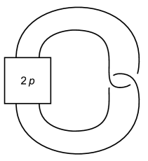
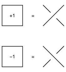
Figure 1: Knot diagram of the twist knot $K^{\mathrm{twist}}_{p}$ (left), where the box represents repeated half-twists, according to the legend on the right.

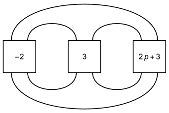
Figure 2: Knot diagram of the $(-2,3,2p+3)$-pretzel knot $K^{\mathrm{pretz}}_{p}$; again the boxes represent repeated half-twists as described in Fig. 1.

We investigate the colored Jones polynomials of two families of knots that appeared previously in the literature: twist knots [17] and pretzel knots [14], see Figures 1 and 2. While it is very difficult to compute the colored Jones polynomial for an arbitrary given knot, one can give simpler formulas for these two families. For example, the $n$-th entry $J^{\mathrm{twist}}_{p}(n)$ of the colored Jones polynomial for the $p$-th twist knot $K^{\mathrm{twist}}_{p}$ is given by the double sum

$$\sum_{k=0}^{n}\sum_{j=0}^{k}(-1)^{j+1}q^{k+pj(j+1)+j(j-1)/2}\bigl{(}q^{2j+1}-1\bigr{)}\frac{\bigl{(}q^{1-n};q\bigr{)}_{\!k}\,\bigl{(}q^{1+n};q\bigr{)}_{\!k}\,\bigl{(}q^{k-j+1};q\bigr{)}_{\!j}}{\bigl{(}q;q\bigr{)}_{\!k+j+1}}.$$

From this representation it is a routine task (but possibly computationally expensive) to compute a $q$-holonomic recurrence equation for $J^{\mathrm{twist}}_{p}(n)$ when $p$ is a fixed integer. This can be done either by $q$-holonomic summation methods (as implemented in the qMultiSum package [25] or HolonomicFunctions package [20]) or by guessing (as implemented in the Guess package [19]). For example, for $p=-1$ we obtain the inhomogeneous $q$-recurrence

$$q^{2n+2}\left(q^{n+2}-1\right)\left(q^{2n+1}-1\right)J^{\mathrm{twist}}_{-1}(n+2)\;+\;\left(q^{n+1}-1\right)^{2}\left(q^{n+1}+1\right)\bigl{(}q^{n+1}+{}$$

$$+q^{2n+1}+q^{2n+3}+q^{3n+3}-q^{4n+4}-1\bigr{)}J^{\mathrm{twist}}_{-1}(n+1)\;+\;q^{2n+2}\left(q^{n}-1\right)$$

$$\times\left(q^{2n+3}-1\right)J^{\mathrm{twist}}_{-1}(n)\;=\;q^{n+1}\left(q^{n+1}+1\right)\left(q^{2n+1}-1\right)\left(q^{2n+3}-1\right).$$

Garoufalidis and Sun have computed such an inhomogeneous $q$-recurrence equation for each twist knot $K^{\mathrm{twist}}_{p}$ with $-15\leq p\leq 15$; the recurrences are available in electronic form from [17]. Similarly, the $q$-recurrences satisfied by $J^{\mathrm{pretz}}_{p}(n)$ for $-5\leq p\leq 5$ are available from [14]. By observing that in each recurrence the term $f(n+d)$ has (among others) a factor $(q^{n+d}-1)$, it is reasonable to perform the substitution $f(n)\to f(n)/(q^{n}-1)$, according to Conjecture 5.1. In the rest of this section, we only use operators that were normalized in this way.

We have implemented Algorithms 4.10 and 4.13 in Mathematica by using the packages HolonomicFunctions [20] and Singular [18]; the source code and a demo notebook are freely available as part of the supplementary electronic material [21]. Note that we also modify Algorithm 4.13 for desingularization of the trailing coefficient of a given $q$-difference operator in the corresponding package and notebook. We give an example about finding desingularized operators in the context of knot theory.

Example 5.2.

We consider the $q$-difference operators that correspond to the homogeneous parts of the recurrences for the colored Jones polynomials of the knots $K^{\mathrm{twist}}_{-1}$, $K^{\mathrm{twist}}_{2}$, $K^{\mathrm{pretz}}_{-2}$, and $K^{\mathrm{pretz}}_{2}$. For example, the operator $P^{\mathrm{twist}}_{-1}$ corresponds, after normalization, to the left-hand side of the above $q$-recurrence for $J^{\mathrm{twist}}_{-1}(n)$:

$$P^{\mathrm{twist}}_{-1}={} q^{2}x^{2}\bigl{(}qx^{2}-1\bigr{)}{\partial}^{2}-{}$$

$$(qx-1)(qx+1)\bigl{(}q^{4}x^{4}-q^{3}x^{3}-q^{3}x^{2}-qx^{2}-qx+1\bigr{)}{\partial}+{}$$

$$q^{2}x^{2}\bigl{(}q^{3}x^{2}-1\bigr{)}$$

For space reasons, the other three operators are displayed in abbreviated form only:

$$P^{\mathrm{twist}}_{2} =(qx-1)(qx+1)(qx^{2}-1){\partial}^{3}+\ell_{1,2}{\partial}^{2}+\ell_{1,1}{\partial}+\ell_{1,0},$$

$$P^{\mathrm{pretz}}_{-2} =(qx-1)(qx+1)(qx^{2}-1){\partial}^{3}+\ell_{2,2}{\partial}^{2}+\ell_{2,1}{\partial}+\ell_{2,0},$$

$$P^{\mathrm{pretz}}_{2} =q^{59}(qx-1)(q^{2}x+1){\partial}^{6}+\ell_{3,5}{\partial}^{5}+\ell_{3,4}{\partial}^{4}+\cdots+\ell_{3,0},$$

where $\ell_{i,j}\in{\mathbb{K}}[q][x]$. We now apply our desingularization algorithm to each of the four operators.

1. By using Theorem 4.8, we obtain an order bound $b$ for a desingularized operator (see Table 1).

2. Using Gröbner bases, we can find a generating set of $M_{b}$. Since the size of this generating set is large, we do not display it here.

3. By [29, Lemma 3.3.3], we find the generator of $I_{b}$ (see Table 1).

4. It is straightforward to see that in each of the four cases, this single generator is the element in $I_{b}$ with minimal degree in $x$.

5. Tracing back to the computation of steps (3) and (4), we find a $q$-difference operator $L\in{\mathbb{K}}[q][x,{\partial}]$ of $\operatorname{Cont}(P)$, which is of the following form:

   $$L^{\mathrm{twist}}_{-1} =q^{4}x^{2}{\partial}^{3}-\left(q^{9}x^{4}-q^{7}x^{3}-q^{5}x^{3}-q^{5}x^{2}-q^{4}x^{2}-q^{2}x+1\right){\partial}^{2}-{}$$

   $$\qquad q^{4}x\left(q^{4}x^{4}-q^{3}x^{3}-q^{3}x^{2}-q^{2}x^{2}-q^{2}x-x+q\right){\partial}+q^{7}x^{3},$$

   $$L^{\mathrm{twist}}_{2} ={\partial}^{5}+p_{1,4}{\partial}^{4}+p_{1,3}{\partial}^{3}+\cdots+p_{1,0},$$

   $$L^{\mathrm{pretz}}_{-2} ={\partial}^{5}+p_{2,4}{\partial}^{4}+p_{2,3}{\partial}^{3}+\cdots+p_{2,0},$$

   $$L^{\mathrm{pretz}}_{2} ={\partial}^{10}+p_{3,9}{\partial}^{9}+p_{3,8}{\partial}^{8}+\cdots+p_{3,0},$$

   where $p_{i,j}\in{\mathbb{K}}[q][x]$.

We observe that in all four examples the minimal order for desingularized operators matches with the predicted order bound, i.e., the bound is tight in these cases. This can be seen by inspecting the $(b-1)$-st coefficient ideal $I_{b-1}$ (see Table 1). We conclude that the sequences that are annihilated by the four operators, respectively, consist indeed of (Laurent) polynomials, provided that the initial values have this property as well.

	$P^{\mathrm{twist}}_{-1}$	$P^{\mathrm{twist}}_{2}$	$P^{\mathrm{pretz}}_{-2}$	$P^{\mathrm{pretz}}_{2}$
order bound $b$	3	5	5	10
generator of $I_{b}$	$I_{3}=\langle x^{2}\rangle$	$I_{5}=\langle 1\rangle$	$I_{5}=\langle 1\rangle$	$I_{10}=\langle 1\rangle$
generator of $I_{b-1}$		$\langle q^{3}x^{2}-1\rangle$	$\langle q^{3}x^{2}-1\rangle$	$\langle q^{4}x-1\rangle$

Table 1: Computations for Example 5.2

Example 5.3.

By applying our desingularization algorithm to the unnormalized $q$-recurrences of $J^{\mathrm{twist}}_{p}(n)$ for the same values of $p$ as in the previous example, we can prove that in these instances the operators are not completely desingularizable, therefore confirming part (2) of Conjecture 5.1.

Since Algorithms 4.10 and 4.13 involve Gröbner bases computations, it is rather inefficient to find desingularized operators when the size of the given $q$-difference operator is large. Alternatively, we may apply guessing [19] to compute a desingularized operator of a given $q$-difference operator, once we derive an order bound by Theorem 4.8.

In order to illustrate the guessing approach, we focus on a slightly modified problem, namely that of finding bimonic recurrence equations: we want to completely desingularize both the leading and the trailing coefficient, i.e., after desingularization these two coefficients should have the form $q^{an+b}$ for some integers $a,b\in{\mathbb{N}}$. The existence of such a recurrence equation certifies that the bi-infinite sequence $\bigl{(}f(n)\bigr{)}{}_{n\in{\mathbb{Z}}}$ has only Laurent polynomial entries. Note that this approach is also suited for inhomogeneous recurrences.

It works as follows: assume we are given a (possibly inhomogeneous) recurrence

$$\underbrace{p_{-1}(q,q^{n})+\sum_{i=0}^{r}p_{i}(q,q^{n})f(n+i)}_{\textstyle=:R(n)}=0,$$

with $r\geq 0$ and $p_{i}\in{\mathbb{K}}[q,q^{n}]$ for $-1\leq i\leq r$. Define the polynomial $c(q,q^{n})\in{\mathbb{K}}[q,q^{n}]$ by

$$c(q,q^{n})=\frac{\operatorname{lcm}\bigl{(}p_{0}(q,q^{n}),p_{r}(q,q^{n})\bigr{)}}{q^{an+b}}$$

with integers $a,b\in{\mathbb{N}}$ chosen such that $c(q,q^{n})$ is neither divisible by $q$ nor by $q^{n}$. The goal is to determine polynomials $u_{i}(q,q^{n})\in{\mathbb{K}}[q,q^{n}]$ such that the coefficients $\ell_{i}(q,q^{n})$, $-1\leq i\leq r+s$, in the linear combination

$$\sum_{i=0}^{s}u_{i}(q,q^{n})R(n+i)=\ell_{-1}(q,q^{n})+\sum_{i=0}^{r+s}\ell_{i}(q,q^{n})f(n+i)$$

are all divisible by $c(q,q^{n})$. Hence, we make an ansatz for the coefficients of the linear combination, instead of trying to guess the desingularized operator directly. The latter would be much more costly to compute (compare the number of green dots with the number of blue dots in Figure 3). The procedure is sketched in Algorithm 5.4. We have implemented it in Mathematica; the source code and a demo notebook are freely available as part of the supplementary electronic material [22].

Algorithm 5.4.

Given a recurrence $R(n)=p_{-1}(q,q^{n})+\sum_{i=0}^{r}p_{i}(q,q^{n})f(n+i)$ and a factor $c(q,q^{n})$ that is to be removed. Compute $u_{i}\in{\mathbb{K}}[q,q^{n}]$ such that $\sum_{i=0}^{s}u_{i}(q,q^{n})R(n+i)=c(q,q^{n})\bigl{(}\ell_{-1}(q,q^{n})+\sum_{i=0}^{r+s}\ell_{i}(q,q^{n})f(n+i)\bigr{)}$ for some polynomials $\ell_{i}\in{\mathbb{K}}[q,q^{n}]$.

1. Make an ansatz of the form $A=\sum_{i=0}^{s}\sum_{j=e_{i}}^{d_{i}}c_{i,j}(q)q^{jn}R(n+i)$ (one may note that the coefficients $c_{0,j}$ and $c_{s,j}$ are already prescribed (up to a constant multiple in ${\mathbb{K}}(q)$) by the choice of $c(q,q^{n})$.

2. Write $A$ in the form $A=a_{-1}(q,q^{n})+\sum_{i=0}^{r+s}a_{i}(q,q^{n})f(n+i)$.

3. For $-1\leq i\leq r+s$ compute the remainder of the polynomial division of $a_{i}(q,q^{n})$ by $c(q,q^{n})$, regarded as polynomials in $q^{n}$.

4. Perform coefficient comparison in these remainders with respect to $q^{n}$.

5. Solve the resulting linear system over ${\mathbb{K}}(q)$ for the unknowns $c_{i,j}\in{\mathbb{K}}[q]$ (we may clear denominators since the system is homogeneous).

6. Return $u_{i}(q,q^{n})=\sum_{j=e_{i}}^{d_{i}}c_{i,j}(q)q^{jn}$.

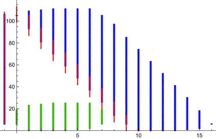
Figure 3: $q^{n}$-support of the coefficients $p_{-1},\dots,p_{9}\in{\mathbb{Q}}[q,q^{n}]$ of the inhomogeneous $q$-recurrence for $K^{\mathrm{pretz}}_{3}$ (red), $q^{n}$-support of the coefficients $u_{0},\dots,u_{7}$ (green), and $q^{n}$-support of the resulting bimonic recurrence (blue), represented by the coefficients $\ell_{-1},\dots,\ell_{16}$; the horizontal axis gives the index of the coefficient, the vertical axis the exponent of $q^{n}$.

It is interesting to note that our computed bimonic recurrences reveal certain symmetries in their coefficients, more precisely, they are kind of palindromic. For example, the bimonic $q$-recurrence that we found for $J^{\mathrm{pretz}}_{-2}(n)$, written in the form

$$\sum_{j=0}^{9}\ell_{-1,j}(q)q^{jn}+\sum_{i=0}^{5}\sum_{j=0}^{9}\ell_{i,j}(q)q^{jn}f(n+i)$$

has the following palindromicity properties ($0\leq i\leq 5$, $0\leq j\leq 9$).

$$\ell_{i,j}=q^{5j-i-20}\ell_{5-i,9-j}\quad\text{and}\quad\ell_{-1,j}=-q^{5j-25}\ell_{-1,10-j}.$$

This phenomenon is illustrated in Table 2. It is also visible in Figure 3 but on a different example. The occurrence of palindromic operators in the context of knot theory has been studied in more detail in [15]. Indeed, if we use the bimonic recurrence to define the sequence $f(n)=(q^{n}-1)J^{\mathrm{pretz}}_{-2}(n)$ for $n\leq 0$ then we see that this sequence is palindromic:

$$f(n)=-q^{n}\,f(-n)\quad\text{for all }n\in{\mathbb{N}}.$$

$$\begin{array}[]{@{}l|r@{\,\cdot\,}lr@{\,\cdot\,}lr@{\,\cdot\,}lr@{\,\cdot\,}lr@{\,\cdot\,}lr@{\,\cdot\,}lr@{\,\cdot\,}l@{}}&\lx@intercol\hfil 1\hfil\lx@intercol&\lx@intercol\hfil f(n)\hfil\lx@intercol&\lx@intercol\hfil f(n+1)\hfil\lx@intercol&\lx@intercol\hfil f(n+2)\hfil\lx@intercol&\lx@intercol\hfil f(n+3)\hfil\lx@intercol&\lx@intercol\hfil f(n+4)\hfil\lx@intercol&\lx@intercol\hfil f(n+5)\hfil\lx@intercol\\[2.15277pt] \hline\cr\rule{0.0pt}{12.0pt}q^{0n}&\lx@intercol\hfil\hfil\lx@intercol&\lx@intercol\hfil\hfil\lx@intercol&\lx@intercol\hfil\hfil\lx@intercol&\lx@intercol\hfil\hfil\lx@intercol&-1&2^{4}&1&2^{3}&\lx@intercol\hfil\hfil\lx@intercol\\ q^{1n}&\lx@intercol\hfil\hfil\lx@intercol&\lx@intercol\hfil\hfil\lx@intercol&\lx@intercol\hfil\hfil\lx@intercol&-1&2^{12}&18&2^{7}&-1&2^{1}&\;1&2^{0}\\ q^{2n}&1&2^{9}&\lx@intercol\hfil\hfil\lx@intercol&\lx@intercol\hfil\hfil\lx@intercol&33&2^{10}&13&2^{7}&24&2^{5}&\lx@intercol\hfil\hfil\lx@intercol\\ q^{3n}&153&2^{8}&\lx@intercol\hfil\hfil\lx@intercol&1&2^{16}&5&2^{12}&177&2^{9}&3&2^{9}&\lx@intercol\hfil\hfil\lx@intercol\\ q^{4n}&93&2^{11}&\lx@intercol\hfil\hfil\lx@intercol&-1&2^{17}&89&2^{13}&3&2^{14}&3&2^{13}&\lx@intercol\hfil\hfil\lx@intercol\\ q^{5n}&\lx@intercol\hfil\hfil\lx@intercol&\lx@intercol\hfil\hfil\lx@intercol&3&2^{17}&3&2^{17}&89&2^{15}&-1&2^{18}&\lx@intercol\hfil\hfil\lx@intercol\\ q^{6n}&-93&2^{16}&\lx@intercol\hfil\hfil\lx@intercol&3&2^{18}&177&2^{17}&5&2^{19}&1&2^{22}&\lx@intercol\hfil\hfil\lx@intercol\\ q^{7n}&-153&2^{18}&\lx@intercol\hfil\hfil\lx@intercol&24&2^{19}&13&2^{20}&33&2^{22}&\lx@intercol\hfil\hfil\lx@intercol&\lx@intercol\hfil\hfil\lx@intercol\\ q^{8n}&-1&2^{24}&1&2^{20}&-1&2^{20}&18&2^{25}&-1&2^{29}&\lx@intercol\hfil\hfil\lx@intercol&\lx@intercol\hfil\hfil\lx@intercol\\ q^{9n}&\lx@intercol\hfil\hfil\lx@intercol&\lx@intercol\hfil\hfil\lx@intercol&1&2^{27}&-1&2^{27}&\lx@intercol\hfil\hfil\lx@intercol&\lx@intercol\hfil\hfil\lx@intercol&\lx@intercol\hfil\hfil\lx@intercol\\ \end{array}$$

Table 2: Coefficients of the bimonic $q$-recurrence for $J^{\mathrm{pretz}}_{-2}(n)$; for space reasons only the evaluations for $q=2$ are given. In order to reveal the underlying symmetry, common powers of $q$ are kept as powers of $2$; for example, the entry $24\cdot 2^{5}$ in the last-but-one column comes from the coefficient of $q^{2n}f(n+4)$ which is $q^{5}(q^{4}+q^{3}-q+2)$. The first column corresponds to the inhomogeneous part.

We have applied Algorithm 5.4 to all recurrences associated to the twist knots $K^{\mathrm{twist}}_{p}$ for $-14\leq p\leq 15$ and to some of the pretzel knots $K^{\mathrm{pretz}}_{p}$. All these results can be found in the supplementary electronic material [22].

6 Conclusion

In this paper, we determine a generating set of the $q$-Weyl closure of a given univariate $q$-difference operator, and compute a desingularized operator whose leading coefficient has minimal degree in $q$. Moreover, we use our algorithms to certify that several instances of the colored Jones polynomial are Laurent polynomial sequences. A challenging topic for future research would be to consider the corresponding problems in the multivariate case.

Another direction of research we want to consider in the future is the desingularization problem for linear Mahler equations [23], which attracted quite some interest in the computer algebra community recently, see for example [8]. Mahler equations arise in the study of automatic sequences, in the complexity analysis of divide-and-conquer algorithms, and in some number-theoretic questions.

Acknowledgment

The authors would like to thank Stavros Garoufalidis for providing the examples of Section 5 and for enlightening discussions on the knot theory part. We are also grateful to the anonymous referee for the detailed report and for numerous valuable comments.

References

[1]
S. A. Abramov, M. Barkatou, and M. van Hoeij.
Apparent singularities of linear difference equations with polynomial
coefficients.
AAECC, 117–133, 2006.
[2]
S. A. Abramov and M. van Hoeij.
Desingularization of linear difference operators with polynomial coefficients.
In Proc. of ISSAC’99, 269–275, New York, NY,USA, 1999, ACM.
[3]
S. A. Abramov, P. Paule, and M. Petkovšek.
-Hypergeometric solutions of -difference equations.
In Discrete Mathematics, 194:3–22, 1999.
[4]
M. A. Barkatou and S. S. Maddah.
Removing apparent singularities of systems of linear differential
equations with rational function coefficients.
In Proc. of ISSAC’15, 53–60, New York, NY,
USA, 2015, ACM.
[5]
S. Chen, M. Jaroschek, M. Kauers, and M. F. Singer.
Desingularization explains order-degree curves for Ore operators.
In Proc. of ISSAC’13, 157–164, New York, NY,
USA, 2013, ACM.
[6]
S. Chen, M. Kauers, Z. Li, and Y. Zhang.
Apparent singularities of D-finite systems.
arXiv 1705.00838, pages 1–26, 2017.
[7]
S. Chen, M. Kauers, and M. F. Singer.
Desingularization of Ore operators.
J. Symb. Comput., 74:617–626, 2016.
[8]
F. Chyzak, T. Dreyfus, P. Dumas and M. Mezzarobba.
Computing solutions of linear Mahler equations.
arXiv 1612.05518, pages 1–42, 2016.
[9]
F. Chyzak, P. Dumas, H. Le, J. Martin, M. Mishna and B. Salvy.
Taming apparent singularities via Ore closure.
Manuscript, 2010.
[10]
F. Chyzak and B. Salvy.
Non-commutative elimination in Ore algebras proves multivariate
identities.
J. Symb. Comput. , 26:187–227, 1998.
[11]
E. Ince.
Ordinary differential equations.
Dover, 1926.
[12]
S. Garoufalidis.
Conjecture about the existence of bimonic recurrences for the colored Jones polynomial.Personal communication, 2018.
[13]
S. Garoufalidis and C. Koutschan.
Twisting -holonomic sequences by complex roots of unity.In Proc. of ISSAC’12, 179–186, New York, NY, USA, 2012, ACM.
[14]
S. Garoufalidis and C. Koutschan.
The non-commutative -polynomial of pretzel knots.
Experimental Mathematics, 21(3):241–251, 2012.
http://www.koutschan.de/data/pretzel/
[15]
S. Garoufalidis and C. Koutschan.
Irreducibility of -difference operators and the knot .
Algebraic & Geometric Topology, 13(6):3261–3286, 2013.
[16]
S. Garoufalidis and T. T. Q. Lê.
The colored Jones function is -holonomic.
Geometry and Topology, 9:1253–1293, 2005.
[21]
C. Koutschan and Y. Zhang.
Supplementary electronic material 1 to the article Desingularization in the -Weyl algebra.
https://yzhang1616.github.io/qdesing.html
[22]
C. Koutschan and Y. Zhang.
Supplementary electronic material 2 to the article Desingularization in the -Weyl algebra.
http://www.koutschan.de/data/qdesing/
[23]
K. Mahler.
Arithmetische Eigenschaften der Lösungen einer Klasse von Funktionalgleichungen.
Mathematische Annalen, 103 (1929), no. 1, 532.
[24]
Y. Man and F. Wright.
Fast polynomial dispersion computation and its application to indefinite summation.
In Proc. of ISSAC’94, 175–180 , New York, NY, USA, 1994, ACM.
[25]
A. Riese.
qMultiSum—A Package for Proving -Hypergeometric Multiple Summation Identities.
Journal of Symbolic Computation, 35:349–376, 2003.
[26]
D. Robertz.
Formal algorithmic elimination for PDEs.
Springer, 2014.
[27]
R. P. Stanley.
Differentiably finite power series.
European Journal of Combinatorics, 1:175–188, 1980.
[28]
Y. Zhang.
Contraction of Ore ideals with applications.
In Proc. of ISSAC’16, 413–420, New York, NY, USA, 2016, ACM.