Abstract

Background

The acoustic damping in gas turbines and aero-engines relies to a great extent on acoustic liners that consists of a cavity and a perforated face sheet. The prediction of the impedance of the liners by direct numerical simulation is nowadays not feasible due to the hundreds to thousands repetitions of tiny holes. We introduce a procedure to numerically obtain the Rayleigh conductivity for acoustic liners for viscous gases at rest, and with it define the acoustic impedance of the perforated sheet.

Results

The proposed method decouples the effects that are dominant on different scales: (a) viscous and incompressible flow at the scale of one hole, (b) inviscid and incompressible flow at the scale of the hole pattern, and (c) inviscid and compressible flow at the scale of the wave-length. With the method of matched asymptotic expansions we couple the different scales and eventually obtain effective impedance conditions on the macroscopic scale. For this the effective Rayleigh conductivity results by numerical solution of an instationary Stokes problem in frequency domain around one hole with prescribed pressure at infinite distance to the aperture. It depends on hole shape, frequency, mean density and viscosity divided by the area of the periodicity cell. This enables us to estimate dissipation losses and transmission properties, that we compare with acoustic measurements in a duct acoustic test rig with a circular cross-section by DLR Berlin.

Conclusions

A precise and reasonable definition of an effective Rayleigh conductivity at the scale of one hole is proposed and impedance conditions for the macroscopic pressure or velocity are derived in a systematic procedure. The comparison with experiments show that the derived impedance conditions give a good prediction of the dissipation losses.

Keywords

Acoustic liner, Perforated plates, Multiscale analysis, Rayleigh conductivity, Impedance conditions.

MSC classification codes

35Q30, 35B27, 74Q15, 76M50

1 Introduction

The safe and stable operation of modern low-emission gas turbines and aero-engines crucially depends on the acoustic damping capability of the combustion system components. Hereby, so called bias flow liner – consisting of a cavity and a perforated face sheet with additional cooling air flow – play a significant role. Since decades the damping performance prediction of these bias flow liner under all possible flow conditions remains a major challenge. However, due to the higher tendency of low-emission, lean burn combustion concepts for combustion instabilities the prediction of the acoustic bias flow liner impedance and therewith its damping performance is a very important prerequisite for the engine design process. Several analytical and semi-empirical models for the impedance description of bias flow liner were developed in the past (see also [1]). This work focuses on the numerical simulation of the acoustic characteristics of bias flow liner applying multi-scale modeling.

In principal all theoretical approaches are based on the formulation of the Rayleigh conductivity $K_{R}$ [2, 3] which describes the ratio of the fluctuating volume flow $Q(t)$ through a hole to the driving pressure difference $P^{-}(t)-P^{+}(t)$ across the hole:

$$K_{R}:=\frac{\rho_{0}\partial_{t}Q(t)}{P^{-}(t)-P^{+}(t)},$$ (1)

and has the dimensions of length. One major challenge in the model description of the Rayleigh conductivity represents the definition or the specification of the pressure difference since, above and below the perforated liner face-sheet the pressure is not necessarily constant rather a function of the distance from the hole. Here, the present work applying a multiscale asymptotic model will provide an exactly defined solution. More precisely, the Rayleigh conductivity of a single hole in an array of holes is distributed over the whole liner area. In this way the effective Rayleigh conductivity

$$k_{R}=\frac{K_{R}}{A_{\delta}}$$ (2)

as quotient of the Rayleigh conductivity of one hole and the area $A_{\delta}$ of one periodicity cell of the array is introduced that has the dimensions of one over length. Using the effective Rayleigh conductivity the liner impedance can be determined like later shown for example in equation (21).

2 Methods

We consider acoustic liner that consist of a wall or part of a wall with a periodic dense array of equisized and equishaped holes with an characteristic periodicity that is proportional to a small parameter $\delta>0$. The holes may not be of cylindrical shape and even tilted in general. For sake of simplicity we consider the perforated wall $\Omega_{\text{liner}}^{\delta}$ with a circular cross-section of inner radius $R_{\textrm{d}}$, while noting that the proposed procedure to define the Rayleigh conductivity and impedance conditions do not depend on the choice of the cross-section, but only on the hole pattern and hole shape and can be directly transfered to other cross-sections like rectangular.

To derive the impedance conditions we let the parameter $\delta$ of the hole period tending zero – so the number holes increases accordingly – while the inner and outer diameter of the cross section are scaled like $\delta^{2}$ as well as the thickness of the perforated wall, see Fig. 1. As $\delta\to 0$, the holes merge and the domain $\Omega^{\delta}_{\text{liner}}$ degenerates to an interface $\Gamma_{\text{liner}}$ on which we will prescibe the impedance conditions representing the correct disspation behaviour of the acoustic liner. For the circular liner the limit interface domain $\Gamma_{\text{liner}}$ is an cylinder of radius $R_{\textrm{d}}$. As it simplifies the derivation and impedance condition greatly we assume that the area of the periodicity cell of the periodic array $A_{\delta}=\delta^{2}$.

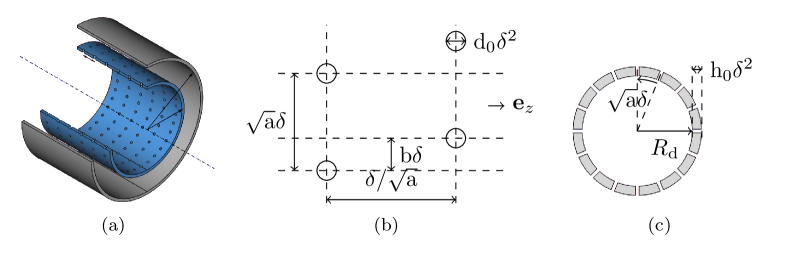
Figure 1: (a) Simplified geometry of a combustion liner for acoustic studies. (b) flattened liner. (c) view along a cross-section.

This liner shall be embedded in a duct domain $\Omega$ and the computational domain is $\Omega^{\delta}:=\Omega\setminus\Omega_{\text{liner}}^{\delta}$ for every $\delta>0$, i.e., , the duct domain without the multi-perforated wall. On this domain we introduce as viscoacoustic model the linearized compressible Navier-Stokes equations in frequency domain in a uniform and stagnant media for a source term ${\mathbf{f}}(t,x)={\operatorname{Re}}({\mathbf{f}}(x)\exp(-\imath\omega t))$ with an angular frequency $\omega>0$:

$$-\imath\omega{\mathbf{v}}^{\delta}+\tfrac{1}{\rho_{0}}\nabla p^{\delta}-\nu(\delta)\operatorname{\Delta}{\mathbf{v}}^{\delta}-\nu^{\prime}(\delta)\nabla\operatorname{div}{\mathbf{v}}^{\delta} ={\mathbf{f}},\quad\text{in }\Omega^{\delta},$$ (3a)

$$-\imath\omega p^{\delta}+\rho_{0}c^{2}\operatorname{div}{\mathbf{v}}^{\delta} =0,\quad\text{in }\Omega^{\delta},$$ (3b)

$${\mathbf{v}}^{\delta} =\bm{0},\quad\text{on }\partial\Omega^{\delta},$$ (3c)

with the acoustic velocity $${\mathbf{v}}^{\delta} p^{\delta} \rho_{0}>0 c \nu(\delta),\nu^{\prime}(\delta)>0 \delta\to 0 \delta^{4} z\pm\infty$$, the acoustic pressure , the mean density , the speed of sound , the kinematic and secondary viscosities . We scale the viscosities for like such that the size of the viscous boundary layers remain asymptotically the same at the scale of a single hole. If the duct is modelled to be of infinite extend then additional conditions at infinity have to be posed, e.g., , for a channel of constant cross section with infinite extend in these conditions are

$$\lim_{z\to\pm\infty}p^{\delta} =0.$$ (3d)

Moreover, we assume the souce to be located away from the perforated wall such that ${\mathbf{f}}=0$ in a neighbourhood.

In the following section we study the solution of the viscoacoustic model in three different geometrical scales beginning at the scale of one hole, pursuing with the scale of one period of the hole array and concluding with the macroscopic scale on which the impedance conditions follow.

2.1 Microscopic scale: the near field around one hole

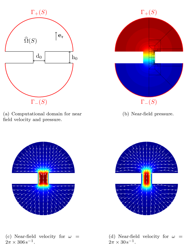
Figure 2: (a) Computational domain for the near field problem around a single hole. (b) The near field pressure (real part) for the liner configuration DC006 (see Table 1) at $\omega=2\pi\times 306\,\text{s}^{-1}$ using $S=40$. (c),(d) The near field velocity (imaginary part) for the same configuration as (b) and for $\omega=2\pi\times 30\,\text{s}^{-1}$. Here, the color coding corresponds to the amplitude and the arrows to the direction of the velocity.

In the vicinity of one hole that tends to a point ${\mathbf{x}}_{\Gamma}$ on the interface $\Gamma_{\text{liner}}$ we use the local coordinate ${\mathfrak{X}}:=({\mathfrak{r}},{\mathfrak{y}},{\mathfrak{z}})=((r-R_{\textrm{d}})/\delta^{2},r\theta/\delta^{2},z/\delta^{2})$. As $\delta\to 0$, the hole variable ${\mathfrak{X}}$ occupies the whole unbounded domain $\widehat{\Omega}$ defined by (see Fig. 2a)

$$\widehat{\Omega}=\big{\{}({\mathfrak{r}},{\mathfrak{y}},{\mathfrak{z}})\in{\mathbb{R}}^{3}\text{ such that }{\mathfrak{r}}<0\text{ or }{\mathfrak{r}}>{\mathrm{h}}_{0}\}\cup\widehat{\Omega}_{\text{hole}}\$$ (4)

where $\widehat{\Omega}_{\text{hole}}$ is the scaled domain representing one hole, and we assume $\bm{0}\in\widehat{\Omega}_{\text{hole}}$. For instance a vertical cylindrical hole of diameter ${\mathrm{d}}_{0}\delta^{2}$ can be represented by $\widehat{\Omega}_{\text{hole}}=\{({\mathfrak{r}},{\mathfrak{y}},{\mathfrak{z}})\in{\mathbb{R}}^{3}\text{ such that }0\leq{\mathfrak{r}}\leq{\mathrm{h}}_{0}\text{ and }{\mathfrak{y}}^{2}+{\mathfrak{z}}^{2}<\frac{1}{4}{\mathrm{d}}_{0}^{2}\}$.

Close to one hole of the perforated liner, we represent the solution $({\mathbf{v}}^{\delta},p^{\delta})$ of (3) as

$${\mathbf{v}}^{\delta} =\bm{\mathfrak{v}}_{0}({\mathbf{x}}_{\Gamma},{\mathfrak{X}})+O(\delta)\ ,$$ (5)

$$p^{\delta} ={\mathfrak{p}}_{0}({\mathbf{x}}_{\Gamma},{\mathfrak{X}})+\delta^{2}{\mathfrak{p}}_{1}({\mathbf{x}}_{\Gamma},{\mathfrak{X}})+O(\delta^{3})\ ,$$

where the near field corrector terms $(\bm{\mathfrak{v}}_{0},{\mathfrak{p}}_{0},{\mathfrak{p}}_{1})$ do not depend on $\delta$. The scaling of the second corrector for the pressure as $\delta^{2}$ is due to the associated scaling of the size of the holes.

Now, inserting expansion (5) into the viscoacoustic model (3) and identifying formally terms of same powers of $\delta$ results first in the fact that ${\mathfrak{p}}_{0}({\mathbf{x}}_{\Gamma},{\mathfrak{X}})$ is a constant function in ${\mathfrak{X}}$, and then in a product representation of the near-field corrector

$$\left(\bm{\mathfrak{v}}_{0}({\mathbf{x}}_{\Gamma},{\mathfrak{X}}),{\mathfrak{p}}_{1}({\mathbf{x}}_{\Gamma},{\mathfrak{X}})\right)=c({\mathbf{x}}_{\Gamma})\left(\tilde{\bm{\mathfrak{v}}}({\mathfrak{X}}),\tilde{{\mathfrak{p}}}({\mathfrak{X}})\right)\ ,$$

where $c({\mathbf{x}}_{\Gamma})$ allows for a slow variation of near field velocity and pressure along the wall.

The near field profiles $(\tilde{\bm{\mathfrak{v}}},\tilde{{\mathfrak{p}}})$ are solution of the instationary Stokes problem

$$-\imath\omega\tilde{\bm{\mathfrak{v}}}+\tfrac{1}{\rho_{0}}\nabla\tilde{{\mathfrak{p}}}-\nu_{0}\operatorname{\Delta}\tilde{\bm{\mathfrak{v}}} =\bm{0}, \quad\text{in }\widehat{\Omega},$$ (6a)

$$\operatorname{div}\tilde{\bm{\mathfrak{v}}} =0, \quad\text{in }\widehat{\Omega},$$ (6b)

$$\tilde{\bm{\mathfrak{v}}} =\bm{0}, \quad\text{on }\partial\widehat{\Omega},$$ (6c)

where $$\nabla \operatorname{div} \Delta {\mathfrak{X}} \nu_{0} -{\rm i}\omega\tilde{\bm{\mathfrak{v}}}$$, and are the gradient, divergence and Laplace operator in (cf. [4, Sec. 2.1.6] in time-domain). The near field velocity profile is incompressible on the scale of one hole and fulfills together with the near field pressure profile the Stokes equations with an at the scale of one hole significant viscosity and the additional term that reflects a time shift between excitation and excited fields. These equations are completed by Dirichlet jump conditions at infinity

$$\lim_{S\to\infty}\tilde{{\mathfrak{p}}}_{|\Gamma_{\pm}(S)} =\pm\tfrac{1}{2}\ ,$$ (6d)

that act as a excitation from far away and will be used for the matching with the mesoscopic scale (see Sec. 2.2). Here,

$$\Gamma_{\pm}(S)=\left\{({\mathfrak{r}},{\mathfrak{y}},{\mathfrak{z}})\in\widehat{\Omega},\pm{\mathfrak{r}}>{\mathfrak{r}}_{\pm}\text{ and }({\mathfrak{r}}-{\mathfrak{r}}_{\pm})^{2}+{\mathfrak{y}}^{2}+{\mathfrak{z}}^{2}=S^{2}\right\},$$ (7)

with ${\mathfrak{r}}_{-}=0$ and ${\mathfrak{r}}_{+}={\mathrm{h}}_{0}$, are the two half-spheres (see Fig. 2a) that are moved towards infinity.

Note that in problem (6) the term $-\nu_{0}^{\prime}\nabla\operatorname{div}\tilde{\bm{\mathfrak{v}}}$ that would appear in the first line cancels out due to the divergence free condition (6b). Moreover, note that the term $-\nu_{0}\Delta\tilde{\bm{\mathfrak{v}}}$ can be replaced by $\nu_{0}\operatorname{{\bf curl}}\operatorname{{\bf curl}}\tilde{\bm{\mathfrak{v}}}$ and so only the vorticity part of the velocity $\tilde{\bm{\mathfrak{v}}}$ will exhibit a viscosity boundary layer as we will see later.

Problem (6) is a classical saddle-point problem and admits a unique solution stated by the following

Proposition 2.1.

There exists a unique solution $(\tilde{\bm{\mathfrak{v}}},\tilde{{\mathfrak{p}}})\in(\mathrm{H}^{1}(\widehat{\Omega}))^{3}\times\bm{\mathcal{V}}(\widehat{\Omega})$ of (6), where $\bm{\mathcal{V}}(\widehat{\Omega})=\left\{P\in\mathrm{H}_{\text{loc}}^{1}(\widehat{\Omega})\text{ such that }\left\lVert\nabla P\right\rVert_{\mathrm{L}^{2}(\widehat{\Omega})}<\infty\right\}.$

Note, that the pressure space $\bm{\mathcal{V}}(\widehat{\Omega})$ allows for a constant behavior towards infinity.

With the near field velocity profile $\tilde{\bm{\mathfrak{v}}}$ defined by (6) we can define in analogy to the Rayleigh conductivity a posteriori the quantity

$$k_{R}:=\lim_{S\to\infty}\frac{\imath\omega\rho_{0}}{2}\Big{(}\int_{\Gamma_{+}(S)}\tilde{\bm{\mathfrak{v}}}\cdot{\mathbf{n}}-\int_{\Gamma_{-}(S)}\tilde{\bm{\mathfrak{v}}}\cdot{\mathbf{n}}\Big{)}$$ (8)

using the volume flux towards infinity in a symmetric way. Here, ${\mathbf{n}}$ is the outer normal vector. In this way, the quantity $k_{R}$ is a mapping of a constant near field pressure at infinity to the flux at infinity. To see the analogy it suffices to consider time harmonic fields varying like $\exp(-\imath\omega t)$, the volume flux $Q(t)$ through the aperture counted positively along the direction of the ${\mathbf{e}}_{\mathfrak{r}}$ axis to be the same as the volume flux through the surface $\Gamma_{+}(S)$ (respectively $\Gamma_{-}(S)$), counted positively (resp. negatively) along the direction of the normal vector ${\mathbf{n}}$, and to compare (1) and (8).

Note, that the normal component of the near field velocity profile $\bm{\mathfrak{v}}$ decays like $1/S^{2}$ towards infinity and combines different behaviour close to and away from the wall (see Fig. 2(c) and (d)). This behaviour can be rigorously justified with similar techniques as in [5, 6].

For the usual definition of the Rayleigh conductivity $K_{R}$ it is not evident where the difference of the pressure – as it varies locally – and the volume flux – as in the original acoustic equations the fluid is compressible – shall be evaluated. The quantity $k_{R}$ is, however, clearly defined by (6) and (8) as the near field pressure tends to constant values for $|{\mathfrak{X}}|\to\infty$ and as the near field velocity is incompressible. This results from the separation of the effects at the different length scales, namely viscous incompressible behaviour in the vicinity of the holes versus inviscid, compressible behaviour away from them, due to the asymptotic ansatz. As the near field profiles are defined in local coordinates ${\mathfrak{X}}$ it has the dimensions of one over length and we denote it as effective Rayleigh conductivity of the liner.

The definition of the effective Rayleigh conductivity $k_{R}$ can be used for inviscid fluids as well for which $\nu_{0}=0$ if the no-slip boundary conditions (6c) are replaced by $\bm{\mathfrak{v}}\cdot{\mathbf{n}}=0$.

2.2 Mesoscopic scale: the hole pattern

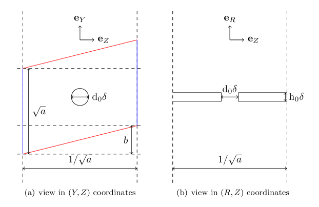
Figure 3: Representation of the periodicity cell ${\mathcal{B}}^{\delta}$ associated to the intermediate scale

Pursuing with the scale of one period of the hole array and in the vicinity of one hole that tends to ${\mathbf{x}}_{\Gamma}$, we use the local coordinate ${\mathbf{X}}:=(R,Y,Z)=((r-R_{\textrm{d}})/\delta,r\theta/\delta,z/\delta)$. We consider for fixed $\delta>0$ the infinite periodicity cell

$${\mathcal{B}}^{\delta} ={\mathcal{B}}^{\delta}_{+}\cup{\mathcal{B}}^{\delta}_{-}\cup\delta\widehat{\Omega}_{\text{hole}}$$ (9)

where ${\mathcal{B}}^{\delta}_{\pm}=\big{\{}(R,Y,Z)\in{\mathbb{R}}^{3}\text{ such that }|Y-bZ|<\tfrac{\sqrt{{\mathrm{a}}}}{2},|Z|<\tfrac{1}{2\sqrt{a}},\pm R>R_{\pm}^{\delta}\big{\}}$ with $R_{-}^{\delta}=0$, $R_{+}^{\delta}={\mathrm{h}}_{0}\delta$ are two semi-infinite parallelepipeds whose opposite lateral faces $|Z|=\tfrac{1}{2\sqrt{a}}$ and $|Y-bZ|=\tfrac{\sqrt{{\mathrm{a}}}}{2}$ are considered to be identified with each other such that ${\mathcal{B}}^{\delta}_{\pm}$ and so ${\mathcal{B}}^{\delta}$ are topologically equivalent to a torus. With the cross-section of the periodicity cell

$$\Gamma(S)=\{(R,Y,Z)\in{\mathbb{R}}^{3}\text{ such that }|Y-bZ|<\tfrac{\sqrt{{\mathrm{a}}}}{2},|Z|<\tfrac{1}{2\sqrt{a}},R=S\}$$

the symmetric difference $A\triangle B:=(A\cup B)\setminus(A\cap B)$ the boundary of the periodicity cell is given as $\partial{\mathcal{B}}^{\delta}=(\Gamma(h_{0}\delta)\cup\Gamma(0))\,\triangle\,\delta\partial\widehat{\Omega}_{\text{hole}}$. It consists of the wall boundary and the boundary of the hole. The periodicity cell ${\mathcal{B}}^{\delta}$ degenerates as $\delta\to 0$ and tends to the union ${\mathcal{B}}^{0}$ of two semi-infinite parallelepipeds ${\mathcal{B}}^{0}_{\pm}$ connected by the point $\bm{0}$, an infinitely small hole.

Inside the periodic array of holes, we represent the solution $({\mathbf{v}}^{\delta},p^{\delta})$ of (3) as

$${\mathbf{v}}^{\delta} ={\mathbf{V}}_{0}^{\delta}({\mathbf{x}}_{\Gamma},{\mathbf{X}})+O(\delta)\ ,$$ (10)

$$p^{\delta} =P_{0}^{\delta}({\mathbf{x}}_{\Gamma},{\mathbf{X}})+\delta P_{1}^{\delta}({\mathbf{x}}_{\Gamma},{\mathbf{X}})+O(\delta^{2})$$

with ${\mathbf{X}}\in{\mathcal{B}}^{\delta}$.

Inserting expansion (10) in problem (3) and identifying formally the terms of same powers of $\delta$ gives that $P_{0}^{\delta}({\mathbf{x}}_{\Gamma},{\mathbf{X}})$ is constant in ${\mathbf{X}}$ and a separation of variables for the mesoscopic corrector as $\big{(}{\mathbf{V}}_{0}^{\delta}({\mathbf{x}}_{\Gamma},{\mathbf{X}}),P_{1}^{\delta}({\mathbf{x}}_{\Gamma},{\mathbf{X}})\big{)}=c({\mathbf{x}}_{\Gamma})\big{(}\bm{\mathcal{V}}^{\delta}({\mathbf{X}}),{\mathcal{P}}^{\delta}({\mathbf{X}})\big{)}$ with the mesoscopic profile $(\bm{\mathcal{V}}^{\delta}$, ${\mathcal{P}}^{\delta})$ satisfying the Darcy-type problem

$$\left\{\begin{aligned} -\imath\omega\bm{\mathcal{V}}^{\delta}+\tfrac{1}{\rho_{0}}\nabla{\mathcal{P}}^{\delta}&=0,\quad\text{in }{\mathcal{B}}^{\delta},\\ \operatorname{div}\bm{\mathcal{V}}^{\delta}&=0,\quad\text{in }{\mathcal{B}}^{\delta},\\ \bm{\mathcal{V}}^{\delta}\cdot{\mathbf{n}}&=0,\quad\text{on }\partial{\mathcal{B}}^{\delta}\ .\end{aligned}\right.$$ (11)

Here, $\nabla$ and $\operatorname{div}$ are the gradient and divergence in ${\mathfrak{X}}$. The formal identification of terms of same power in $\delta$ can be justified despite the fact that the size of the hole depends on $\delta$ as well. For this an additional scale $\eta$ for the size of one hole has to be introduced that is first considered to be independent of $\delta$ due to its different meaning and later fixed to $\delta^{2}$. The expansion (10) is then in $\delta$, where the terms of the expansion depend on $\eta$. For the brevity of the article we have chosen directly $\eta=\delta^{2}$.

Note that (11) is equivalent to an homogeneous Laplace problem with Neumann boundary conditions for the pressure profile ${\mathcal{P}}^{\delta}$, where the velocity profile $\bm{\mathcal{V}}^{\delta}$ can be computed from. Following [7, Proposition 2.2], we can therefore state the following

Proposition 2.2.

For any fixed $\delta>0$, the kernel of problem (11) is of dimension $2$ and spanned by the functions $(\bm{\mathcal{V}}_{\mathcal{N}}^{\delta},{\mathcal{P}}_{\mathcal{D}}^{\delta})=(0,1)$ and $(\bm{\mathcal{V}}_{\mathcal{D}}^{\delta},{\mathcal{P}}_{\mathcal{D}}^{\delta})$ such that ${\mathcal{D}}_{v}^{\delta}$ is constant as $R\to\pm\infty$. Moreover, there exists ${\mathcal{D}}_{\infty}^{\delta}\in{\mathbb{C}}$ such that $(\bm{\mathcal{V}}_{\mathcal{D}}^{\delta},{\mathcal{P}}_{\mathcal{D}}^{\delta})$ admits the following limit behaviour:

$$\bm{\mathcal{V}}_{\mathcal{D}}^{\delta} =\tfrac{1}{\imath\omega}{\mathbf{e}}_{R}+o(1), \quad R\to\pm\infty,$$ (12)

$${\mathcal{P}}_{\mathcal{D}}^{\delta} =\rho_{0}R\pm{\mathcal{D}}_{\infty}^{\delta}+o(1), \quad R\to\pm\infty.$$

It remains to determine the constant ${\mathcal{D}}_{\infty}^{\delta}$, where we are in particular interested in its asymptotic behaviour for $\delta\to 0$. To obtain this behaviour we will match the mesoscopic functions $\bm{\mathcal{V}}_{\mathcal{D}}^{\delta}$ and ${\mathcal{P}}_{\mathcal{D}}^{\delta}$ with the near field profiles $\tilde{\bm{\mathfrak{v}}}$ and $\tilde{{\mathfrak{p}}}$ at half-spheres $\Gamma_{\pm}(s^{\delta})$ of radius $s^{\delta}$ for $\sqrt{\delta}<s^{\delta}<2\sqrt{\delta}$ centered at the aperture $\bm{0}$. First we note that due to the incompressibility and the limit behaviour of $\bm{\mathcal{V}}_{\mathcal{D}}^{\delta}$ for its volume flux over the half-spheres it holds

$$\frac{\imath\omega}{2}\left(\int_{\Gamma_{+}(s^{\delta})}\bm{\mathcal{V}}_{\mathcal{D}}^{\delta}\cdot{\mathbf{n}}-\int_{\Gamma_{-}(s^{\delta})}\bm{\mathcal{V}}_{\mathcal{D}}^{\delta}\cdot{\mathbf{n}}\right)=\frac{\imath\omega}{2}\lim_{S\to\infty}\int_{\Gamma(S)}\bm{\mathcal{V}}_{\mathcal{D}}^{\delta}\cdot{\mathbf{e}}_{R}+\int_{\Gamma(-S)}\bm{\mathcal{V}}_{\mathcal{D}}^{\delta}\cdot{\mathbf{e}}_{R}=1\ .$$

Using this equality, definition (8) of the effective Rayleigh conductivity $k_{R}$, the mesoscopic to microscopic variable change ${\mathfrak{X}}={\mathbf{X}}/\delta$, and matching of the mesoscopic velocity $\bm{\mathcal{V}}_{\mathcal{D}}^{\delta}$ and the near field velocity profile $\tilde{\bm{\mathfrak{v}}}$ we find that

$$\bm{\mathcal{V}}_{\mathcal{D}}^{\delta}({\mathbf{X}})\sim\frac{\rho_{0}}{k_{R}\delta^{2}}\tilde{\bm{\mathfrak{v}}}(\tfrac{{\mathbf{X}}}{\delta})\quad\text{ for }\sqrt{\delta}<|{\mathbf{X}}|<2\sqrt{\delta}\text{ and }\delta\to 0\ .$$

By linearity and using definition of problems (6) and (11), the gradient of the mesoscopic pressure ${\mathcal{P}}_{\mathcal{D}}^{\delta}$ can be matched with the gradient of the near field pressure profile as well. Integrating these gradients, using limit (6d) and Proposition 2.2 leads to

$${\mathcal{P}}_{\mathcal{D}}^{\delta}({\mathbf{X}})\sim\frac{\rho_{0}}{k_{R}\delta}\tilde{{\mathfrak{p}}}(\tfrac{{\mathbf{X}}}{\delta})\sim\pm\frac{\rho_{0}}{2k_{R}\delta}\quad\text{ for }\sqrt{\delta}<|{\mathbf{X}}|<2\sqrt{\delta},\pm R>0\text{ and }\delta\to 0\ .$$

As for $\delta\to 0$ the mesoscopic pressure ${\mathcal{P}}_{\mathcal{D}}^{\delta}$ tends to $\rho_{0}R\pm{\mathcal{D}}^{\delta}_{\infty}$ if $\delta=o(|{\mathbf{X}}|)$ we conclude that

$${\mathcal{D}}_{\infty}^{\delta}=\frac{\rho_{0}}{2k_{R}\delta}+o(\delta^{-1})\ .$$ (13)

This blow up of the coefficient ${\mathcal{D}}_{\infty}^{\delta}$ as $\delta\to 0$ in accordance with its numerical computations based on an asymptotic analysis of (3) with only two scales [8], where the hole size is considered not as a scale but as a parameter.

2.3 Macroscopic scale and impedance conditions

Finally, away from a vicinity of the layer, the solution $({\mathbf{v}}^{\delta},p^{\delta})$ of (3) is represented by

$${\mathbf{v}}^{\delta}({\mathbf{x}}) ={\mathbf{v}}_{0}({\mathbf{x}})+o(1),$$ (14)

$$p^{\delta}({\mathbf{x}}) =p_{0}({\mathbf{x}})+o(1).$$

Inserting this expansion in problem (3) and making a formal identification in terms of powers of $\delta$ gives that $({\mathbf{v}}_{0},p_{0})$ is solution of the classical Helmholtz problem

$$-\imath\omega{\mathbf{v}}_{0}+\tfrac{1}{\rho_{0}}\nabla p_{0} ={\mathbf{f}},\quad\text{in }\Omega\setminus\Gamma_{\text{liner}},$$ (15a)

$$-\imath\omega p_{0}+\rho_{0}c^{2}\operatorname{div}{\mathbf{v}}_{0} =0,\quad\text{in }\Omega\setminus\Gamma_{\text{liner}},$$ (15b)

and a multiscale analysis [9] for rigid walls leads to the boundary conditions

$${\mathbf{v}}_{0}\cdot{\mathbf{n}} =0,\quad\text{on }\partial\Omega\ .$$ (15c)

The limit condition (3d) becomes

$$\lim_{z\to\pm\infty}{\mathbf{v}}_{0}\cdot(\pm 1,0,0)-T_{\pm}^{1}p_{0}=0,$$ (15d)

where $T_{\pm}^{1}$ is the Dirichlet-to-Neumann operator based on the projection on the outgoing propagative modes, see [10, Eq. (2.7)] and [11]. This problem is completed by jump conditions across the interface $\Gamma_{\text{liner}}$. To obtain the conditions we match the macroscopic pressure $p_{0}$ and flux ${\mathbf{v}}_{0}\cdot{\mathbf{n}}$ in a matching zone at distance $\sqrt{\delta}$ to the interface $\Gamma_{\text{liner}}$ to the mesoscopic pressure and velocity functions. For the pressure we find

$$p_{0}({\mathbf{x}})=C_{\mathcal{N}}({\mathbf{x}}_{\Gamma})\,{\mathcal{P}}_{\mathcal{N}}^{\delta}(\tfrac{{\mathbf{x}}-{\mathbf{x}}_{\Gamma}}{\delta})+\delta C_{\mathcal{D}}({\mathbf{x}}_{\Gamma})\,{\mathcal{P}}_{\mathcal{D}}^{\delta}(\tfrac{{\mathbf{x}}-{\mathbf{x}}_{\Gamma}}{\delta})\\ \text{ for }\sqrt{\delta}\leq|{\mathbf{x}}-{\mathbf{x}}_{\Gamma}|\leq 2\sqrt{\delta}\text{ and }\delta\to 0.$$ (16)

with two functions $C_{\mathcal{N}}$, $C_{\mathcal{D}}$ that allow for slow variation along the perforated wall. With the factor $\delta$ the limit $\delta{\mathcal{P}}^{\delta}_{\mathcal{D}}(\frac{{\mathbf{x}}-{\mathbf{x}}_{\Gamma}}{\delta})$ for $\delta\to 0$ remains bounded. Subtracting the two limits of (16) for $\delta\to 0$ we obtain

$$\big{[}p_{0}\big{]}({\mathbf{x}}_{\Gamma}) :=\lim_{\delta\to 0}p_{0}({\mathbf{x}}_{\Gamma}+\sqrt{\delta}{\mathbf{n}})-p_{0}({\mathbf{x}}_{\Gamma}-\sqrt{\delta}{\mathbf{n}})=C_{\mathcal{D}}({\mathbf{x}}_{\Gamma})\frac{\rho_{0}}{k_{R}}\ .$$ (17)

Taking the gradient in ${\mathbf{x}}$ on both sides of (16) and using (15a), the assumption that ${\mathbf{f}}=0$ close to the perforated wall and (11) we find

$${\mathbf{v}}_{0}({\mathbf{x}})\cdot{\mathbf{n}}=\frac{\rho_{0}}{\imath\omega}\nabla p_{0}({\mathbf{x}})\cdot{\mathbf{n}}=\delta C_{\mathcal{D}}({\mathbf{x}}_{\Gamma})\,\frac{\rho_{0}}{\imath\omega}\nabla{\mathcal{P}}_{\mathcal{D}}^{\delta}(\tfrac{{\mathbf{x}}-{\mathbf{x}}_{\Gamma}}{\delta})=C_{\mathcal{D}}({\mathbf{x}}_{\Gamma})\,\bm{\mathcal{V}}_{\mathcal{D}}^{\delta}(\tfrac{{\mathbf{x}}-{\mathbf{x}}_{\Gamma}}{\delta})\\ \text{ for }\sqrt{\delta}\leq|{\mathbf{x}}-{\mathbf{x}}_{\Gamma}|\leq 2\sqrt{\delta}\text{ and }\delta\to 0\ .$$ (18)

As the two limits for $\bm{\mathcal{V}}^{\delta}_{\mathcal{D}}$ for $R\to\pm\infty$ coincide we obtain

$$\big{[}{\mathbf{v}}_{0}\cdot{\mathbf{n}}\big{]}({\mathbf{x}}_{\Gamma}) =0,\quad\text{on }\Gamma_{\text{liner}}\ .$$ (19a)

Finally, taking the average of (18) and the limit $$\delta\to 0$$ gives in view of (17) the impedance conditions

$$\big{[}p_{0}\big{]}({\mathbf{x}}_{\Gamma}) =\frac{\imath\omega\rho_{0}}{k_{R}}\big{<}{\mathbf{v}}_{0}\cdot{\mathbf{n}}\big{>}({\mathbf{x}}_{\Gamma}),\quad\text{on }\Gamma_{\text{liner}}\ .$$ (19b)

Note, that the impedance conditions do not depend on the pattern of the holes, more precisely on the values ${\mathrm{a}}$ and ${\mathrm{b}}$ (see Fig. 1), but only on their area $A_{\delta}$, namely through $\nu_{0}=\nu/A_{\delta}^{2}$ in the computation of the effective Rayleigh conductivity $k_{R}$.

Distinguished limit

Note, that the nature of the impedance condition (19b) is due to the choice of asymptotic scales. It represents a distinguished limit meaning that different choice would lead to one of the trivial conditions $\big{[}p_{0}\big{]}({\mathbf{x}}_{\Gamma})=0$ (transparent wall) or $\big{<}{\mathbf{v}}_{0}\cdot{\mathbf{n}}\big{>}({\mathbf{x}}_{\Gamma})=0$ (rigid wall). If we would scale the diameter of each hole like $\varepsilon(\delta)$ as well as the thickness of the perforated wall such that $\delta^{2}=o(\varepsilon(\delta))$ then we would obtain transparent wall conditions in the limit $\delta\to 0$. A contrario, the impedance conditions become rigid wall conditions if we would use the scaling $\varepsilon(\delta)=o(\delta^{2})$. The choice of asymptotic scales was already stated in [12] for infinitely thin perforated wall and the Stokes flows.

Acoustic Impedance

The nature of the impedance conditions is known in the literature: the notion of impedance can be found in the works of Webster in the 1910s [13]. More precisely, he defines the normalized specified acoustic impedance $\zeta$ by (note there is a complex conjugate and a different sign due to the different choice of the time-dependency convention)

$$\zeta:=-\frac{\overline{\big{[}p_{0}\big{]}}}{c\rho_{0}\overline{\big{<}{\mathbf{v}}_{0}\cdot{\mathbf{n}}\big{>}}}\ .$$ (20)

For the derived impedance conditions (19b) and by identification, the normalized specified acoustic impedance for perforated walls is given by

$$\zeta=\frac{\imath\omega}{c\overline{k_{R}}}=\frac{\imath\omega k_{R}}{c|k_{R}|^{2}}\ .$$ (21)

The resistance ${\operatorname{Re}}(\zeta)$ and the reactance ${\operatorname{Im}}(\zeta)$ are positive quantities when $k_{R}$ has a positive real part and a negative imaginary part. Moreover in the inviscid case $k_{R}$ is a positive real number, so that the normalized specified acoustic impedance $\zeta$ is purely a reactance.

Formulation in pressure only

One can also remark that Problem (15) can be formulated in terms of pressure only: equations (15a)– (15d) give

$$\Delta p_{0}+\tfrac{\omega^{2}}{c^{2}}p_{0} =\operatorname{div}{\mathbf{f}}, \text{in }\Omega\setminus\Gamma_{\text{liner}},$$ (22a)

$$\nabla p_{0}\cdot{\mathbf{n}} =0, \text{on }\partial\Omega,$$

$$\lim_{z\to\pm\infty}\pm\partial_{z}p_{0}-\imath\omega\rho_{0}T_{\pm}^{1}p_{0} =0,$$

and impedance conditions (19a)-(19b) are written in terms of the pressure as

$$\big{[}\nabla p_{0}\cdot{\mathbf{n}}\big{]}({\mathbf{x}}_{\Gamma})=0\quad\text{and}\quad\big{<}\nabla p_{0}\cdot{\mathbf{n}}\big{>}({\mathbf{x}}_{\Gamma})=k_{R}\big{[}p_{0}\big{]}({\mathbf{x}}_{\Gamma})\ .$$ (22b)

This kind of conditions were proposed for the inviscid case [14], where $$k_{R}$$ turns out to be the effective plate compliance.

3 Results and discussion

In this section, we are interested by the numerical computation of the effective Rayleigh conductivity $k_{R}$, the computation of dissipation losses in acoustic ducts with the impedance conditions and comparison with data from experimental measurements.

3.1 Numerical computation of $k_{R}$

The effective Rayleigh conductivity $k_{R}$ is defined through the solution of the near field velocity and pressure profiles in the unbounded domain $\widehat{\Omega}$ around a single hole. To compute $k_{R}$ numerically we truncate the unbounded domain, on which we use the finite element method for discretization and propose an extrapolation procedure to increase the accuracy.

First, we define the truncated domain

$$\widehat{\Omega}(S)=\widehat{\Omega}\cap\big{(}\max(|{\mathfrak{X}}-(0,0,0)|,|{\mathfrak{X}}-({\mathrm{h}}_{0},0,0)|)<S\big{)}$$ (23)

of $\widehat{\Omega}$ for a given truncation radius $S>0.5\sqrt{{\mathrm{d}}_{0}^{2}+{\mathrm{h}}_{0}^{2}}$ (see Fig. 2(a)). It has two artificial boundaries $\Gamma_{\pm}(S)$ that are no boundaries of $\widehat{\Omega}$. We restrict the problem (6) to $\widehat{\Omega}(S)$ and $\partial\widehat{\Omega}(S)\cap\partial\widehat{\Omega}$, and we approximate the conditions (6d) by setting

$$\tilde{{\mathfrak{p}}}_{|\Gamma_{\pm}(S)}=\pm\tfrac{1}{2}.$$

From the resolution of the truncated problem we compute the approximated Rayleigh conductivity $k_{R}(S)$ taking as well an approximation of (8), namely

$$k_{R}(S):=\frac{\imath\omega\rho_{0}}{2}\Big{(}\int_{\Gamma_{+}(S)}\tilde{\bm{\mathfrak{v}}}\cdot{\mathbf{n}}-\int_{\Gamma_{-}(S)}\tilde{\bm{\mathfrak{v}}}\cdot{\mathbf{n}}\Big{)},$$ (24)

Its approximated value $k_{R}(S)$ tends to the Rayleigh conductivity $k_{R}$ as $1/S$ as illustrated in Fig. 4. This first-order convergence can be explained with a rigorous analysis of the solution of problem (6) towards infinity using the Mellin transform [15] and showing that the solution of this problem on $\Gamma_{\pm}(S)$ is a superposition of a radial expansion with respect to $1/S$ and of a cartesian expansion with terms decaying exponentially with respect to the distance to the boundary. Similar analyses were performed for the Poisson and Helmholtz problems in conical domains with a rough periodic boundary [5] or perforated wall [6].

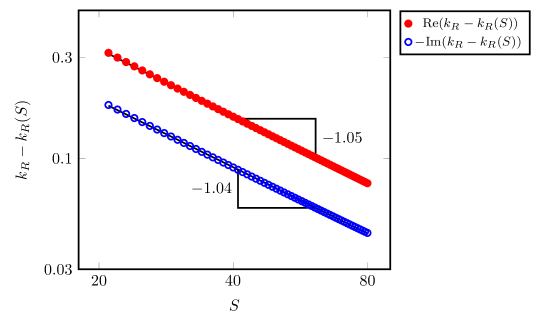
Figure 4: Convergence of the real and imaginary parts of the approximated Rayleigh conductivity $k_{R}(S)$ to its limit value $k_{R}=4.513-1.210\imath$ in dependence of the truncation radius $S$ for the liner DC006 at frequency $f=306\,\text{Hz}$ (see Table 1).

As, more precisely, the Rayleigh conductivity $k_{R}$ can be expanded in powers of $1/S$ we use an extrapolation in $1/S$ of first order approximations $k_{R}(S)$ for different truncation radia $S$ to obtain a second or higher order approximation of the limit value $k_{R}$.

For the particular case of a straight cylindrical hole that is without loss of generality centered at ${\mathfrak{y}}={\mathfrak{z}}=0$, the domain $\widehat{\Omega}(S)$ is invariant under rotation around the ${\mathfrak{r}}$ axis as well as the solution of the problem (6) for the near field profiles. Hence, the finite element method in two dimensions can be used for the numerical resolution in a 2D axis-symmetry setting. To resolve the boundary layer of size $\sqrt{\nu_{0}/\omega}$ on the wall boundary (cf. [4, Sec. 3.1]) we use the $hp$-adaptive strategy of Schwab and Suri [16] (see the mesh shown in Fig. 2(b)).

Config.	number of	longitudinal	azimuthal	hole	liner	$\sigma$
	holes (longitudinal,	inter-hole	inter-hole	diameter	thickness
	azimuthal)	distance $\delta/\sqrt{{\mathrm{a}}}$ (mm)	distance $\sqrt{{\mathrm{a}}}\delta$ (mm)	${\mathrm{d}}_{0}\delta^{2}$ (mm)	${\mathrm{h}}_{0}\delta^{2}$ (mm)	%
DC006	(7,52)	8.5	8.45	1	1	1.1
DC007	(3,20)	22	21.99	2.5	1	1.0
DC008	(7,52)	8.5	8.45	2.5	1	6.8
DC009	(3,20)	22	21.99	1	1	0.2

Table 1: Liner configurations. The length of the liner is $L=60\,\text{mm}$. The value of the viscosity is $\nu(\delta)=1.4660\times 10^{-5}\,\text{m}^{2}/\text{s}$. For all these configurations $b=0.5\sqrt{{\mathrm{a}}}$.

For four liner configurations, see Table 1, from experimental studies [1, 17] we have computed the near field velocity and pressure profiles and so the effective Rayleigh conductivity. The relative kinematic viscosity $\nu_{0}$ is computed as quotient of the kinematic viscosity $\nu=1.4660\times 10^{-5}\,\text{m}^{2}/\text{s}$ of air at $15^{\circ}\mathrm{C}$ divided by the period $\delta$ to the power of four. In Fig. 2(b) and Fig. 2(c) we illustrate the near field pressure and velocity profiles $\tilde{{\mathfrak{p}}}$ and $\tilde{\bm{\mathfrak{v}}}$ for the liner DC006 at frequency $306\,\text{Hz}$ using a truncation radius $S=40$. It is visible that the pressure decays almost linearly inside the cylindrical hole, but also the behaviour at distance to the hole. Moreover, the pressure shows close to the rim of the cylinder an edge singularity (i.e., a corner singularity for the 2D axis-symmetric problem) that is resolved numerically by the hp-adaptive refinement strategy. The near velocity profile shows a flux from all sides to and through the hole. It appears that the outward flux of the imaginary part of $\tilde{\bm{\mathfrak{v}}}$ over $\Gamma_{+}(S)$ is negative (resp. positive over $\Gamma_{-}(S)$) corresponding to a positive real part of the approximate Rayleigh conductivity $k_{R}(S)$ (see (24)) and so of the Rayleigh conductivity $k_{R}$. This is in line with the inviscid case, where $k_{R}$ is real and positive. Moreover, we see the higher velocity amplitude inside the hole that decays towards its boundaries. This boundary layer phenomena is more visible for lower frequencies (see Fig. 2(d)), where one also see a local change of the velocity direction on the wall boundary.

In Fig. 5, we plot the effective Rayleigh conductivity $k_{R}$ as a function of the frequency $f:=\tfrac{\omega}{2\pi}$ for different liner configurations given in Table 1. As expected, following the remark on the normalized specified acoustic impedance $\zeta$, the real part of $k_{R}$ is positive and its imaginary part is negative. One can also remark that for liner configurations DC006 and DC007, that have a close value of the porosity $\sigma$ but quite different hole repartition and hole diameter, their Rayleigh conductivities differ significantly in both their real and imaginary part.

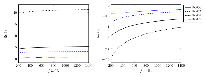
Figure 5: Real and imaginary parts of $k_{R}$ in dependence of the frequency $f=\tfrac{\omega}{2\pi}$.

In Fig. 6, we show the computed normalized specific acoustic impedance $\zeta$ for the liner configuration DC006 in comparison with the Melling model (see [18] and [17, Eq. (12)]), that is given an analytic formula. For the latter an effective kinematic viscosity $\tilde{\nu}(\delta):=2.179\nu(\delta)$ is used that shall incorporate also thermal conductivity losses near a highly conducting wall, see [19, p. 239] and [1, p. 62]. We plotted the Rayleigh conductivities obtained from our model with this effective kinematic viscosity. The reactance predicted by the two models are very close, where the resistence differs by up to $20\%$. The importance of taking the thermal conductivity losses into account will be seen in comparison with the measurements and be discussed later in Sec. 3.3.

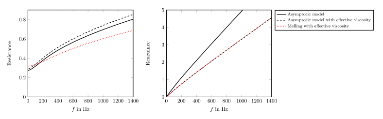
Figure 6: Comparison of the impedance with the normalized specific resistance (left) and the normalized specific reactance (right) computed by our model and Melling model as function of the frequency $f=\tfrac{\omega}{2\pi}$ for the liner configuration DC006. As Melling model uses an effective viscosity taking into account thermal conductivity losses we show the impedance for our model with the effective viscosity as well.

3.2 Dissipation losses in acoustic ducts

3.2.1 Experimental Setup and Analysis

The experimental study is performed in the duct acoustic test rig with a circular cross-section (DUCT-C) at DLR Berlin at ambient conditions. The setup of the test rig is illustrated in Fig. 7. It allows high precision acoustic measurements of the damping performance of various liner configurations, including grazing and bias flow.

Figure 7: Schematic setup of the Duct Acoustic Testrig (DUCT-C) with speakers $A$ and $B$, and microphones 1-12. The anechoic terminations at both ends are not shown.

The test duct consists of two symmetric measurement sections (section 1 and section 2 in Fig. 7) of 1200 mm length each. They have a circular cross-section with a radius $R_{\textrm{d}}$ of 70 mm. In order to minimize the reflection of sound at the end of the duct back into the measuring section the test duct is equipped with anechoic terminations at both ends (not shown in Fig. 7). Their specifications follow the ISO 5136 standard. The damping module is a chamber of 60 mm. It has a circular cross-section with a radius of 120 mm.

A total of 12 microphones are mounted flush with the wall of the test duct. They are installed at different axial positions upstream and downstream of the damping module and are distributed exponentially with a higher density towards the damping module. Two microphones are installed opposite of each other at the same axial position close to the signal source. As evanescent modes become more prominent in the vicinity of the source, their influence is reduced significantly by using the average value of these two microphones for the analysis. This technique helps to reduce the errors for frequencies approaching the cut-on frequency of the first higher order mode and thus, extends the frequency range for accurate results.

At the end of each section a loudspeaker is mounted at the circumference of the duct ($A$ and $B$ in Fig. 7). They deliver the test signal for the damping measurements. The signal used here is a multi-tone sine signal. All tonal components of the signal are in the plane wave range. The signal has been calibrated in a way that the amplitude of each tonal component inside the duct is about 102 dB.

The microphones used in these measurements are 1/4” G.R.A.S. type 40BP condenser microphones. Their signals are recorded with a 16 track OROS OR36 data acquisition system with a sampling frequency of 8192 Hz. The source signals for the loudspeakers are recorded on the remaining tracks. The test signal is produced by an Agilent 33220A function generator. The signals are fed through a Dynacord L300 amplifier before they power the Monacor KU-516 speakers.

For each configuration two different sound fields are excited consecutively in two separate measurements (index a and b). Speaker A is used in the first measurement and in the second measurement the same signal is fed into speaker B. Then, the data of section 1 and section 2 (index 1 and 2) are analyzed separately. This results in four equations for the complex sound pressure amplitudes for each section and measurement for $j=a,b$:

$$\hat{p}_{1j}(z) =\hat{p}_{1j}^{+}e^{\imath\omega z/c}+\hat{p}_{1j}^{-}e^{-\imath\omega z/c}$$ (25a)

$$\hat{p}_{2j}(z) =\hat{p}_{2j}^{+}e^{\imath\omega(z-L)/c}+\hat{p}_{2j}^{-}e^{-\imath\omega(z-L)/c}$$ (25b)

$\hat{p}^{+}$ and $\hat{p}^{-}$ are the complex amplitudes of the downstream and upstream traveling waves.

The recorded microphone signals are transformed into the frequency domain using the method presented by Chung [20]. This method rejects uncorrelated noise, e.g., turbulent flow noise, from the coherent sound pressure signals. Therefore, the sound pressure spectrum of one microphone is determined by calculating the cross-spectral densities between three signals, where one signal serves as a phase reference. In our case the phase reference signal is the source signal of the active loudspeaker. As a result we obtain a phase-correlated complex sound pressure spectrum for each microphone signal.

According to Eqs. (25a)-(25b) the measured acoustic signal is a superposition of two plane waves traveling in opposite direction. In order to determine the downstream and upstream propagating portions of the wave in each section, a mathematical model is fitted to the acoustic microphone data. This model considers viscous and thermal conductivity losses at the duct wall. They are included in the wave number with the following attenuation factor $\alpha$ as proposed by Kirchhoff [21]:

$$\alpha=\frac{1}{cR_{\textrm{d}}}\sqrt{\frac{\nu\omega}{2}}\left(1+\frac{\gamma-1}{\sqrt{Pr}}\right)$$ (26)

with the duct radius $r$, the speed of sound $c$, the kinematic viscosity $\nu$, the angular frequency $\omega$ (as in Eq. (3)), the heat capacity ratio $\gamma$, and the Prandtl number $Pr$. As a result of this least-mean-square fit, the four complex sound pressure amplitudes $\hat{p}_{1}^{+}$, $\hat{p}_{1}^{-}$, $\hat{p}_{2}^{+}$ and $\hat{p}_{2}^{-}$ are identified at position $z=0$ for both measurements. These sound pressure amplitudes are related to each other via the reflection and transmission coefficients of the test object. This is illustrated in Fig. 8 for the two different measurements $A$ and $B$. In order to calculate the reflection and transmission coefficients $r^{+}$, $r^{-}$, $t^{+}$, and $t^{-}$ from the sound pressure amplitudes the following four relations can be derived for $j=a,b$:

$$\hat{p}_{1j}^{-}=r^{+}\hat{p}_{1j}^{+}+t^{-}\hat{p}_{2j}^{-}$$ (27a)

$$\hat{p}_{2j}^{+}=r^{-}\hat{p}_{2j}^{-}+t^{+}\hat{p}_{1j}^{+}$$ (27b)

Figure 8: Illustration of the sound filed in the duct for measurements $A$ and $B$ by means of the sound pressure amplitudes $\hat{p}$, the reflection coefficient $r$, the transmission coefficient $t$, and the end reflection $r_{e}$

The equations from both measurements are combined and solved for the reflection

$$r^{+}=\frac{\hat{p}_{1a}^{-}\hat{p}_{2b}^{-}-\hat{p}_{1b}^{-}\hat{p}_{2a}^{-}}{\hat{p}_{1a}^{+}\hat{p}_{2b}^{-}-\hat{p}_{1b}^{+}\hat{p}_{2a}^{-}}\quad\quad r^{-}=\frac{\hat{p}_{2b}^{+}\hat{p}_{1a}^{+}-\hat{p}_{2a}^{+}\hat{p}_{1b}^{+}}{\hat{p}_{1a}^{+}\hat{p}_{2b}^{-}-\hat{p}_{1b}^{+}\hat{p}_{2a}^{-}}$$ (28)

and transmission coefficients

$$t^{+}=\frac{\hat{p}_{2a}^{+}\hat{p}_{2b}^{-}-\hat{p}_{2b}^{+}\hat{p}_{2a}^{-}}{\hat{p}_{1a}^{+}\hat{p}_{2b}^{-}-\hat{p}_{1b}^{+}\hat{p}_{2a}^{-}}\quad\quad t^{-}=\frac{\hat{p}_{1a}^{+}\hat{p}_{1b}^{-}-\hat{p}_{1b}^{+}\hat{p}_{1a}^{-}}{\hat{p}_{1a}^{+}\hat{p}_{2b}^{-}-\hat{p}_{1b}^{+}\hat{p}_{2a}^{-}}$$ (29)

in downstream and upstream direction, respectively. The advantage of combining the two measurements is that the resulting coefficients are independent from the reflection of sound at the duct terminations. These end-reflections are contained in the sound pressure amplitudes, but do not need to be calculated explicitly. Moreover in the case of a uniform and stagnant flow these coefficients do not depend on the direction we consider, i.e., $r^{-}=r^{+}$ and $t^{-}=t^{+}$.

The dissipation of acoustic energy is expressed by the dissipation coefficient. The dissipation coefficient $\bm{\Delta}$ can be calculated directly from the reflection coefficient $R$ and the transmission coefficient $T$ via an energy balance

$$R^{\pm}+T^{\pm}+\bm{\Delta}^{\pm}=1.$$ (30)

To compute these coefficients, the integration of the acoustic energy flux in a uniform and stagnant flow yields a relation between the acoustic pressure $p$ and acoustic power $P$ quantities(see Blokhintsev [22] and Morfey [23]) :

$$P^{\pm}=\frac{\pi R_{\textrm{d}}^{2}}{2\rho_{0}c}\left|\hat{p}^{\pm}\right|^{2}$$ (31)

Then, the energy coefficients can be given relative to the pressure coefficients as:

$$R^{+} =\tfrac{P_{1}^{-}}{P_{1}^{+}}=\left|r^{+}\right|^{2}$$ (32a)

$$R^{-} =\tfrac{P_{2}^{+}}{P_{2}^{-}}=\left|r^{-}\right|^{2}$$ (32b)

$$T^{+} =\tfrac{P_{2}^{+}}{P_{1}^{+}}=\left|t^{+}\right|^{2}$$ (32c)

$$T^{-} =\tfrac{P_{1}^{-}}{P_{2}^{-}}=\left|t^{-}\right|^{2}$$ (32d)

where the indices $1$ and $2$ refer to section 1 and section 2 of the duct as illustrated in Fig. 8. With the energy balance (30) follows the definition of the energy dissipation coefficient

$$\bm{\Delta}=1-\left(\left|r^{\pm}\right|^{2}+\left|t^{\pm}\right|^{2}\right)$$ (33)

This is an integral value of the acoustic energy that is absorbed while a sound wave is passing the damping module. The dissipation coefficient is used to evaluate the damping performance of the test object.

3.2.2 Numerical simulation of dissipation losses

This setup is also simulated numerically using the equivalent problem (22a)-(22b) for the pressure with a source term corresponding to an incoming field $p_{\mathsf{inc}}(r,\theta,z)=\exp(\imath\omega z/c)$ from the left. The scattered field is computed numerically using the mode matching procedure with $N=5$ modes [24]: we seek for the scattered field $p_{0}$ under the form (see Fig. 9(b))

$$p_{0}(r,\theta,z) =p_{\mathsf{inc}}(r,\theta,z)+\sum_{j=0}^{N-1}\alpha_{j}^{-}\,\psi_{j}(r)\,\exp(-\imath\,\beta_{j}\,z),\quad z<0,$$ (34a)

$$p_{0}(r,\theta,z) =\sum_{j=0}^{N-1}\alpha_{j}^{+}\,\psi_{j}(r)\,\exp(\imath\,\beta_{j}\,z),\quad z>L,$$ (34b)

inside the waveguide part, and under the form

$$p_{0}(r,\theta,z)=\sum_{j=0}^{2N-1}\psi^{\prime}_{j}(r)\big{(}{\alpha^{\prime}_{j}}^{+}\exp(\imath\,\beta_{j}^{\prime}\,z)+{\alpha^{\prime}_{j}}^{-}\exp(\imath\,\beta_{j}^{\prime}\,(L-z))\big{)},\quad 0<z<L,$$ (34c)

inside the duct part. The pairs $$(\beta_{j},\psi_{j}) (\beta_{j}^{\prime},\psi_{j}^{\prime}) p_{\mathsf{inc}} \theta \beta_{j}\in\imath{\mathbb{R}} j\not=0$$ and are solution of a “2D” transverse eigenvalue problem in the wave-guide and liner parts, using the fact that the source term and the geometry are independent of the angle . From the mode matching and assuming that there is only one propagative mode inside the waveguide, i.e.,  for , the energy dissipation coefficient is computed as

$$\bm{\Delta}:=1-\left(|\alpha_{0}^{+}|^{2}+|\alpha_{0}^{-}|^{2}\right),$$ (35)

and corresponds to the energy dissipation coefficient $D^{\pm}$ (Eq. (33)) if both grazing and bias flows are absent.

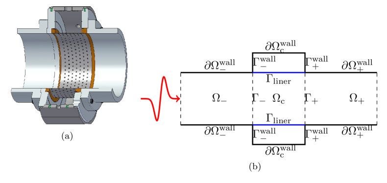
Figure 9: Split of the domain $\Omega$ into the two semi-infinite waveguides $\Omega_{\pm}$ and the multi-perforated liner section $\Omega_{\textrm{c}}$. Impedance transmission conditions on the interface $\Gamma_{\text{liner}}$ approximate the behaviour of the many perforations.

3.3 Numerical results and comparison with experimental data

Figure 10 shows the average dissipation of the different liner configurations (see table 1) in the DUCT-C setup (see figure 8) as a function of the frequency. The average dissipation represents a mean value of the dissipation results for the upstream and downstream acoustic incidence (see section 3.2.1). In a symmetric setup and without grazing flow this is, of course, equal to the dissipation from either side of excitation. The graphs compare the experimental values (symbols), the former theoretical model from Melling [18] (dashed lines) and the here introduced asymptotic model (solid lines). In result, the asymptotic model indicates a better comparison to the experimental values especially for the configurations DC006 (figure 10 (a)) and DC008 (figure 10 (c)) where the Melling model slightly underestimates the dissipation in the frequency range above approximately 400 Hz. For the configuration DC007 with a porosity of 1.0 % and a hole diameter of 2.5 mm both models (Melling and asymptotic) underestimate the maximum dissipation of approximately 0.4 around 400 Hz revealed in the experimental studies.

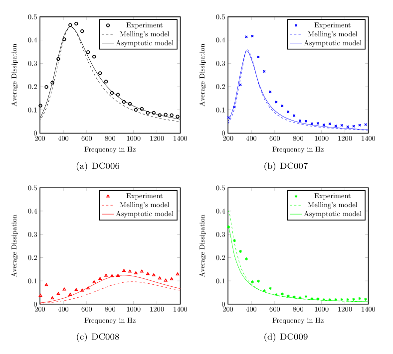
Figure 10: Average dissipation from experiments and numerical modelling plotted over the frequency comparing models for DC006, DC007, DC008, DC009.

4 Conclusions

It has been shown that impedance conditions with one numerically computed parameter – the effective Rayleigh conductivity – can predict well the dissipation losses of acoustic liners. The effective Rayleigh conductivity can be obtained by solving numerically an instationary Stokes problem in frequency domain of one hole with a scaled viscosity in an characteristic infinite domain with prescribed pressure at infinity. For the computation the infinite domain is truncated, where we propose approximative boundary conditions on the artificial boundaries and an extrapolation procedure to save computation time. We decoupled in a systematic way the effects at different scales and derived impedance conditions for the macroscopic pressure or velocity based on a proper matching of pressure and velocity at the different scales. In difference to a direct numerical solution for the acoustic liner the overall computation effort is separated into a precomputation of the effective Rayleigh conductivity and a computation of the Helmholtz equation for the pressure with impedance conditions, where no holes have to be resolved anymore by a finite element mesh. The comparison with measurements in the duct acoustic test rig with a circular cross-section at DLR Berlin show that the dissipation losses based on the impedance conditions with effective Rayleigh conductivity are well predicted. The derivation of the impedance conditions do not depend on the cylindrical shape of the liner and can be used for others shapes like rectangular profiles. The procedure for the computation of the effective Rayleigh conductivity can not only be extented to include thermic effects that are currently only heuristically incorporated, but also nonlinear effects inside the hole that lead to an interaction of frequencies.

References

References

- [1] Lahiri, C.: Acoustic performance of bias flow liners in gas turbine combustors. PhD thesis, Technische Universität Berlin, Berlin, Germany (2014). https://depositonce.tu-berlin.de/handle/11303/4567
- [2] Rayleigh, J.W.S.: On the theory of resonance. Phi. Trans. R. Soc. Lond. 161, 77–118 (1871)
- [3] Rayleigh, J.W.S.: The Theory of Sound, Vol. 2. Dover, New York (1945)
- [4] Popie, V.: Modélisation asymptotique de la réponse acoustique de plaques perforées dans un cadre linéaire avec étude des effets visqueux. PhD thesis, Université de Toulouse, Toulouse, France (2016)
- [5] Nazarov, S.A.: The Neumann problem in angular domains with periodic and parabolic perturbations of the boundary. Tr. Mosk. Mat. Obs. 69, 182–241 (2008)
- [6] Semin, A., Delourme, B., Schmidt, K.: On the homogenization of the Helmholtz problem with thin perforated walls of finite length. ESAIM: Math. Model. Numer. Anal. (2017). Accepted for publication.
- [7] Delourme, B., Schmidt, K., Semin, A.: On the homogenization of thin perforated walls of finite length. Asymptot. Anal. 97(3-4), 211–264 (2016)
- [8] Semin, A., Schmidt, K.: On the homogenization of the acoustic wave propagation in perforated ducts of finite length for an inviscid and a viscous model (Submitted)
- [9] Schmidt, K., Thöns-Zueva, A., Joly, P.: Asymptotic analysis for acoustics in viscous gases close to rigid walls. Math. Models Meth. Appl. Sci. 24(9), 1823–1855 (2014)
- [10] Goldstein, C.I.: A finite element method for solving Helmholtz type equations in waveguides and other unbounded domains. Math. Comp. 39(160), 309–324 (1982)
- [11] Semin, A., Schmidt, K.: Absorbing boundary conditions for the viscous acoustic wave equation. Math. Meth. Appl. Sci. 39(17), 5043–5065 (2016)
- [12] Sanchez-Hubert, J., Sánchez-Palencia, E.: Acoustic fluid flow through holes and permeability of perforated walls. J. Math. Anal. Appl. 87(2), 427–453 (1982)
- [13] Webster, A.G.: Acoustical impedance and the theory of horns and of the phonograph. Proc. Nat. Acad. Sci. 5(7), 275–282 (1919)
- [14] Bendali, A., Fares, M., Piot, E., Tordeux, S.: Mathematical justification of the rayleigh conductivity model for perforated plates in acoustics. SIAM J. Numer. Anal. 73(1), 438–459 (2013)
- [15] Kozlov, V.A., Maz′ya, V.G., Rossmann, J.: Elliptic Boundary Value Problems in Domains with Point Singularities. Mathematical Surveys and Monographs, vol. 52. American Mathematical Society, Providence, RI (1997)
- [16] Schwab, C., Suri, M.: The p and hp versions of the finite element method for problems with boundary layers. Math. Comp. 65(216), 1403–1430 (1996)
- [17] Lahiri, C., Bake, F.: A review of bias flow liners for acoustic damping in gas turbine combustors. J. Sound Vib. 400, 564–605 (2017)
- [18] Melling, T.H.: The acoustic impendance of perforates at medium and high sound pressure levels. J. Sound Vib. 29(1), 1–65 (1973)
- [19] Crandall, I.B.: Theory of Vibrating Systems and Sound. D. Van Nostrand, New York (1926)
- [20] Chung, J.Y.: Rejection of flow noise using a coherence function method. J. Acoust. Soc. Am. 62(2), 388–395 (1977)
- [21] Kirchhoff, G.: Über den Einfluss der Wärmeleitung in einem Gase auf die Schallbewegung. Ann. Phys. Chem. 210(6), 177–193 (1868)
- [22] Blokhintsev, D.I.: Acoustics of a Nonhomogeneous Moving Medium. NACA Technical Memorandum 1399, Washington, DC (1956). Originally published 1946 in russian language
- [23] Morfey, C.L.: Acoustic energy in non-uniform flows. J. Sound Vib. 14(2), 159–170 (1971)
- [24] Semin, A., Thöns-Zueva, A., Schmidt, K.: Simulation of reflection and tranmission properties of multiperforated acoustic liners. In: Prog. Ind. Math. ECMI 2016 (2017). Accepted for publication.