Turbulent heating in an inhomogeneous, magnetized plasma slab

Abstract

Observational evidence in space and astrophysical plasmas with long collisional mean free path suggests that more massive charged particles may be preferentially heated. One possible mechanism for this is the turbulent cascade of energy from injection to dissipation scales, where the energy is converted to heat. Here we consider a simple system consisting of a magnetized plasma slab of electrons and a single ion species with a cross-field density gradient. We show that such a system is subject to an electron drift wave instability, known as the universal instability, which is stabilized only when the electron and ion thermal speeds are equal. For unequal thermal speeds, we find that the instability gives rise to turbulent energy exchange between ions and electrons that acts to equalize the thermal speeds. Consequently, this turbulent heating tends to equalize the component temperatures of pair plasmas and to heat ions to much higher temperatures than electrons for conventional mass-ratio plasmas.

1 Introduction

An interesting and fundamental question in plasma physics is how thermal equilibrium is determined in an essentially collisionless plasma. In such a system, there is no reason a priori to assume that the relative temperatures of the component species will be equal: On the contrary, there are numerous collisionless heating mechanisms that have been identified - shocks, magnetic reconnection, cyclotron resonance (Cranmer et al., 1999), and various forms of turbulent heating (Quataert & Gruzinov, 1999; Howes et al., 2008; Chandran et al., 2010; Barnes et al., 2012), to name a few - and each of these mechanisms may drive temperature separation instead of equilibration. Indeed, evidence from observations of collisionless space and astrophysical plasmas, e.g., the solar wind and accretion flows onto compact objects, suggests that more massive charged particles may be preferentially heated; cf.  (Schmidt et al., 1980; Collier et al., 1996; Kohl et al., 1997; Quataert & Gruzinov, 1999).

A thorough treatment of this problem would require exploration of a parameter space spanning a wide range of plasma $\beta$, electron-ion temperature ratio, energy injection mechanisms, etc., while including all potentially relevant physics present from the macroscopic to microscopic space-time scales. As such a study is infeasible, we choose to focus on a single heating mechanism - turbulent Joule heating - in a simplified system: a two-component plasma immersed in a straight, homogenous magnetic field with a cross-field density gradient. This system supports electron drift waves and is known to be susceptible to the so-called ‘universal’ instability (Galeev et al., 1963; Krall & Rosenbluth, 1965; Landreman et al., 2015; Helander & Plunk, 2015). The universal instability serves as an energy injection mechanism for turbulence at the ion Larmor scale that gives rise to plasma fluctuations that drive cross-field transport and Joule heating (or cooling) of the component plasma species. For sufficiently infrequent collisions, this turbulent heating and transport determines the thermal equilibrium of the plasma.

To guide our study, we note that the universal instability is derived analytically in the limit of disparate ion and electron thermal speeds. As noted in Ref. (Helander, 2014), the universal instability is eliminated for an equal temperature pair plasma, or, more generally, when the ion and electron thermal speeds are equal. In the following sections we analytically and numerically calculate the dependence of the universal instability and resultant turbulent heating on electron-ion temperature ratio for two cases: pair plasmas and conventional mass ratio plasmas. The former case is relevant for proposed experiments in which a small population of positrons is to be added to a pure electron plasma of a different temperature (Pedersen & Boozer, 2002); the latter may provide insight into how astrophysical plasmas can achieve disparate electron and ion temperatures. We introduce the gyrokinetic model used for the analysis in Sec. 2, and we calculate linear growth rates and quasilinear heating and cross-field flux estimates in Sec. 3 before concluding.

2 Model system

We consider a collisionless plasma immersed in a straight, homogeneous magnetic field $\mathbf{B}=B\hat{\mathbf{z}}$ and with a fixed density gradient perpendicular to the field in the $x$-direction. The fixed density gradient could be, e.g., the result of gravitational equilibrium in an astrophysical plasma or of an external particle source in a laboratory plasma. We restrict our attention to electrostatic fluctuations whose frequency is small compared with the Larmor frequency and adopt the gyrokinetic ordering:

$$\epsilon\doteq\frac{\omega}{\Omega_{s}}\sim\frac{k_{\parallel}}{k_{\perp}}\sim\frac{\rho_{s}}{L_{n}}\sim\frac{\delta f_{s}}{f_{s}}\sim\frac{q_{s}\varphi}{T_{s}}\ll 1,$$ (1)

where $\varphi$ is the electrostatic potential fluctuation, $f_{s}$ is the distribution function for species $s$, $\delta f$ is the fluctuating component of $f$, $\omega$ is the characteristic frequency of the fluctuations, $k_{\parallel}$ and $k_{\perp}$ are the associated wavenumbers along and across the mean field, $\Omega_{s}$ is the Larmor frequency for species $s$, $\rho_{s}$ its thermal Larmor radius, $T_{s}$ its temperature, $q_{s}$ its charge, and $L_{n}$ is the mean density gradient scale length.

Applying these orderings to the Fokker-Planck equation and averaging over the rapid gyration of particles about the mean magnetic field results in the gyrokinetic equation,

$$\frac{\partial h_{s}}{\partial t}+v_{\parallel}\frac{\partial h_{s}}{\partial z}+\frac{c}{B}\{\left<\varphi\right>_{\mathbf{R}_{s}},h_{s}\}=-q_{s}\frac{\partial\left<\varphi\right>_{\mathbf{R}_{s}}}{\partial t}\frac{\partial F_{0,s}}{\partial E_{s}}+\frac{c}{B}\frac{\partial\left<\varphi\right>_{\mathbf{R}_{s}}}{\partial y}\frac{\partial F_{0,s}}{\partial x}+C[h_{s}],$$ (2)

where $h_{s}=\delta f_{s}-q_{s}\varphi(\partial F_{0,s}/\partial E_{s})$ is the non-Boltzmann piece of $\delta f_{s}$, $E_{s}=m_{s}v^{2}/2$ is the kinetic energy of species $s$, $m_{s}$ is species mass, $t$ is time, $v_{\parallel}$ is the parallel component of the particle velocity, $c$ is the speed of light, $F_{0,s}$ is the mean component of $f_{s}$, $\{\}$ indicates a Poisson bracket, $\left<\varphi\right>_{\mathbf{R}_{s}}$ is the average of $\varphi$ over Larmor angle at fixed guiding center position $\mathbf{R}_{s}$, and $C[h_{s}]$ represents the effect of Coulomb collisions on species $s$.

The gyrokinetic system is closed by coupling to Poisson’s equation:

$$4\pi\sum_{s}q_{s}\int d^{3}v\delta f_{s}=-\nabla_{\perp}^{2}\varphi,$$ (3)

with $\nabla_{\perp}^{2}=\partial_{x}^{2}+\partial_{y}^{2}$. If the Debye length $\lambda_{s}\doteq(T_{s}/4\pi n_{s}q_{s}^{2})^{1/2}$ is much smaller than the electron Larmor radius, the righthand side of Eq. (3) can be neglected. In this limit Poisson’s equation reduces to the quasineutrality constraint that the total charge density of the plasma is zero. We note that a non-relativistic treatment of finite Debye length effects requires a small plasma beta, $\beta_{s}=8\upi p_{s}/B^{2}\lesssim(v_{\mathrm{th},s}/c)^{2}$, consistent with the electrostatic approximation we employ.

2.1 Turbulent heating and heat transport

By taking fluid moments of the Fokker-Planck equation and closing the system with the gyrokinetic ordering, one obtains an equation for the slow evolution of the mean temperature $T_{s}$:

$$\frac{3}{2}n_{s}\frac{dT_{s}}{dt}+\frac{\partial Q_{s}}{\partial x}=H_{s},$$ (4)

where the cross-field turbulent heat flux $Q_{s}$ and turbulent heating $H_{s}$ are given by

$$Q_{s}=\frac{1}{V}\int d^{3}R\int_{\mathbf{R}}d^{3}v\left(\frac{m_{s}v^{2}}{2}-\frac{3}{2}T_{s}\right)\overline{\left(h_{s}v_{E}\right)}$$ (5)

and

$$H_{s}=\frac{1}{V}\int d^{3}R\int_{\mathbf{R}}d^{3}vq_{s}\overline{\left(h_{s}\frac{\partial\left<\varphi\right>_{\mathbf{R}_{s}}}{\partial t}\right)}.$$ (6)

Here $V$ is the volume of the region over which the spatial integration is performed, the subscript $\mathbf{R}$ on the velocity integration indicates that it is carried out at fixed guiding center, $v_{E}=-(c/B)\partial\varphi/\partial y$ is the x-component of the $E\times B$ drift velocity, and the overline indicates an average over time scales long compared to the fluctuation time $1/\omega$ but short compared to the equilibrium time scale. Note that we have neglected collisional temperature equilibration as we are considering systems with collisional mean free path much longer than any other scales of interest.

An alternative expression for $H_{s}$ is obtained by integrating Eq. (6) by parts in time (Candy, 2013):

$$H_{s}=\frac{1}{2V}\int d^{3}R\int_{\mathbf{R}}d^{3}vq_{s}\overline{\left(h_{s}\frac{\partial\left<\varphi\right>_{\mathbf{R}_{s}}}{\partial t}-\frac{\partial h_{s}}{\partial t}\left<\varphi\right>_{\mathbf{R}_{s}}\right)}.$$ (7)

Substitution of Poisson’s equation (3) in Eq. (7) immediately indicates that the net (species-summed) turbulent heating is zero in the absence of an external energy injection mechanism; i.e., for a two-component plasma, $\overline{H_{i}}=-\overline{H_{e}}$. If trace minority ions are present, one can obtain mass- and charge-dependent scalings for their turbulent heating rates relative to the main ions (Barnes et al., 2012). Expressing Eqs. (5) and (7) in terms of Fourier modes with $h_{s}=\sum_{\mathbf{k}}\tilde{h}_{\mathbf{k},s}(v_{\parallel},v_{\perp},t)\exp(\textnormal{i}\mathbf{k}\cdot\mathbf{R}_{s})$ gives

$$Q_{s}=\textnormal{i}\frac{c}{B}\sum_{\mathbf{k}}k_{y}\int d^{3}vJ_{0}(\alpha_{k_{\perp},s})\frac{m_{s}v^{2}}{2}\overline{\left(\tilde{h}_{\mathbf{k},s}\tilde{\varphi}_{\mathbf{k}}^{*}\right)}\doteq\sum_{\mathbf{k}}\tilde{Q}_{\mathbf{k},s}$$ (8)

and

$$H_{s}=\frac{q_{s}}{2}\sum_{\mathbf{k}}\int d^{3}vJ_{0}(\alpha_{k_{\perp},s})\overline{\left(\frac{\partial\tilde{\varphi}_{\mathbf{k}}^{*}}{\partial t}\tilde{h}_{\mathbf{k},s}-\tilde{\varphi}_{\mathbf{k}}^{*}\frac{\partial\tilde{h}_{\mathbf{k},s}}{\partial t}\right)}\doteq\sum_{\mathbf{k}}\tilde{H}_{\mathbf{k},s},$$ (9)

where $\alpha_{k_{\perp},s}\doteq k_{\perp}v_{\perp}/\Omega_{s}$ and $J_{0}$ is a Bessel function of the first kind.

2.2 Connection to particle transport

The effect of cross-field particle transport is encapsulated in the continuity equation:

$$\frac{\partial n_{s}}{\partial t}+\frac{\partial\Gamma_{s}}{\partial x}=0,$$ (10)

where $n_{s}$ is particle density and

$$\Gamma_{s}=\frac{1}{V}\int d^{3}R\int_{\mathbf{R}}d^{3}v\overline{\left(h_{s}v_{E}\right)}$$ (11)

is the cross-field particle flux. Expanding $\varphi$ and $h$ in terms of Fourier modes gives

$$\Gamma_{s}=\textnormal{i}\frac{c}{B}\sum_{\mathbf{k}}k_{y}\int d^{3}vJ_{0}(\alpha_{k_{\perp},s})\overline{\left(\tilde{h}_{\mathbf{k},s}\tilde{\varphi}_{\mathbf{k}}^{*}\right)}\doteq\sum_{\mathbf{k}}\tilde{\Gamma}_{\mathbf{k},s}.$$ (12)

The particle flux $\Gamma$ can be related to the turbulent heating of Eq. (6) by multiplying the gyrokinetic equation (2) by $\varphi$ and averaging over the phase space:

$$H_{s}=-\frac{1}{V}\int d^{3}R\int_{\mathbf{R}}d^{3}v\left(\frac{T_{s}h_{s}}{F_{0,s}}C[h_{s}]\right)+T_{s}\frac{\partial\ln n_{s}}{\partial x}\Gamma_{s}$$ (13)

Note that the effect of collisions is retained in Eq. (13), but collisional temperature equilibration is neglected in the energy equation (4). This is because the turbulent fluctuations undergo filamentation in phase space and thus tiny collisional deflections in velocity have immediate impact on the turbulent fluctuations – even when the amount of energy that is exchanged in the course of the deflection is negligible. At the small phase space scales where collisional dissipation occurs, the dissipation is effectively diffusive. This gives rise to heating that is positive definite for each species. Furthermore, Poisson’s equation (3) applied to our two-component plasma dictates that $\Gamma_{i}=\Gamma_{e}\doteq\Gamma$ and $n_{i}=n_{e}\doteq n$. Substituting these expressions in Eq. (13) and enforcing $H_{i}=-H_{e}$ results in the constraint that $\Gamma(\partial\ln n/\partial x)\leq 0$ and thus $|H_{s}|\leq T_{s}|\Gamma(\partial\ln n/\partial x)|$. Comparing this inequality with Eqs. (4) and (10), one finds that the timescale associated with turbulent particle transport is always at least as fast as that associated with turbulent heating. One would therefore expect that when turbulent heating drives temperatures apart (as we find below), the effect would be bounded by the rate of transport down the density gradient. Depending on the system under consideration, this may be set by the rate at which plasma is introduced.

3 Linear analysis

If we consider small amplitude perturbations, we may neglect the quadratic nonlinearity and carry out a linear analysis of the gyrokinetic equation. Upon assuming solutions of the form $h_{s}=\sum_{\mathbf{k}}\hat{h}_{\mathbf{k},s}(v_{\parallel},v_{\perp})\exp(i\mathbf{k}\cdot\mathbf{R}_{s}-i\omega t)$, one obtains

$$\hat{h}_{\mathbf{k},s}=\frac{q_{s}\hat{\varphi}_{\mathbf{k}}}{T_{s}}J_{0}(\alpha_{k_{\perp},s})\left(\frac{\omega+\omega_{*,s}}{\omega-k_{\parallel}v_{\parallel}}\right)F_{M,s},$$ (14)

where

$$\omega_{*,s}=\frac{k_{y}\rho_{s}v_{\mathrm{th},s}}{2L_{n,s}}\frac{q_{s}}{|q_{s}|},$$ (15)

$v_{\mathrm{th},s}=2T_{s}/m_{s}$, $m_{s}$ is species mass, $\rho_{s}=v_{\mathrm{th},s}/|\Omega_{s}|$, and $1/L_{n,s}=-\partial\ln n_{s}/\partial x$.

From Poisson’s Equation (3),

$$\int d^{3}v\left(h_{i}-h_{e}\right)=\frac{en}{T_{e}}\left(1+\tau-\lambda_{e}^{2}\nabla_{\perp}^{2}\right)\varphi,$$ (16)

where $\tau\doteq T_{e}/T_{i}$, and we have restricted our attention to a single ion species with proton charge $e$. Substitution of Eq. (14) into Eq. (16) results in the dispersion relation

$$\epsilon(\omega,\mathbf{k})=1+\tau+k_{\perp}^{2}\lambda_{e}^{2}+\left(\zeta_{e}-\frac{k_{y}\rho_{e}}{2k_{\parallel}L_{n}}\right)\Upsilon(k_{y}\rho_{e})Z\left(\zeta_{e}\right)+\tau\left(\zeta_{i}+\frac{k_{y}{\rho_{i}}}{2k_{\parallel}L_{n}}\right)\Upsilon\left(k_{y}\rho_{i}\right)Z\left(\zeta_{i}\right)=0,$$ (17)

where $\zeta_{s}\doteq\omega/k_{\parallel}v_{\mathrm{th},s}$,

$$Z(x)\doteq\textnormal{i}\sqrt{\upi}\textnormal{e}^{-x^{2}}\ \textnormal{erfc}\left(-\textnormal{i}x\right)$$ (18)

is the plasma dispersion function, erfc is the complementary error function, and

$$\Upsilon(x)\doteq\exp\left(-\frac{x^{2}}{2}\right)I_{0}\left(\frac{x^{2}}{2}\right),$$ (19)

with $I_{0}$ a modified Bessel of the first kind. Note that we have used quasineutrality to set $L_{n,i}=L_{n,e}\doteq L_{n}$.

3.1 Quasilinear energy exchange

Using Eq. (14) for $\hat{h}_{\mathbf{k},s}$ in Eq. (9) we get a quasilinear approximation for the energy exchange:

$$\begin{split}\hat{H}_{\mathbf{k},s}&\doteq\frac{\tilde{H}_{\mathbf{k},s}}{nT_{i}}\frac{|L_{n}|}{v_{\mathrm{th},i}}\frac{T_{i}^{2}}{e^{2}|\tilde{\varphi}_{\mathbf{k}}|^{2}}\\ &=\Upsilon(k_{\perp}\rho_{s})k_{\parallel}|L_{n}|\frac{T_{i}}{T_{s}}\textnormal{Re}\left(\zeta_{i}\right)\textnormal{Im}\left(\left(\zeta_{s}+\frac{k_{y}\rho_{s}}{2k_{\parallel}L_{n}}\frac{q_{s}}{|q_{s}|}\right)Z(\zeta_{s})\right),\end{split}$$ (20)

It is straightforward to verify that summing this expression over species and using the dispersion relation of Eq. (17) leads to zero net heating.

This quasilinear estimate provides information about linear phase relationships that indicate the sign of the heating contribution as a function of wavelength. It predicts neither the spectrum nor the saturated heating amplitude in steady-state. As we are primarily interested in the sign of the heating, it is enough to make some assumption about the turbulent heating spectrum; in particular, we assume that the steady-state heating has the same sign as the quasilinear estimate for the mode(s) with the largest linear growth rate. In the following subsections we obtain numerical and approximate analytical solutions for the mode frequencies and associated quasilinear heating in various limits.

3.2 Comparable thermal speeds

We first show that there is no instability, and thus no turbulent heating, if $v_{\mathrm{th},e}=v_{\mathrm{th},i}$. To find the condition for marginal stability, we seek solutions for which $\gamma\doteq\textnormal{Im}\left(\omega\right)=0$. In this case, the plasma dispersion function simplifies to $Z(x)=\sqrt{\upi}\exp(-x^{2})(\textnormal{i}-\textnormal{erfi}\left(x\right))$, with erfi the imaginary error function and $x=\textnormal{Re}\left(\zeta\right)$. The constraint $\textnormal{Im}\left(\epsilon\right)=0$ then gives

$$\left(x_{e}-\frac{k_{y}\rho_{e}}{2k_{\parallel}L_{n}}\right)\Upsilon(k_{y}\rho_{e})\exp(-x_{e}^{2})=-\tau\left(x_{i}+\frac{k_{y}{\rho_{i}}}{2k_{\parallel}L_{n}}\right)\Upsilon\left(k_{y}\rho_{i}\right)\exp(-x_{i}^{2}).$$ (21)

Substituting this expression into the constraint $\textnormal{Re}\left(\epsilon\right)=0$ gives

$$0=1+\tau+k_{\perp}^{2}\lambda_{e}^{2}+\tau\left(x_{i}+\frac{k_{y}{\rho_{i}}}{2k_{\parallel}L_{n}}\right)\Upsilon\left(k_{y}\rho_{i}\right)\upi^{1/2}\exp(-x_{i}^{2})\left(\textnormal{erfi}\left(x_{e}\right)-\textnormal{erfi}\left(x_{i}\right)\right).$$ (22)

When $v_{\mathrm{th},e}=v_{\mathrm{th},i}$, then $x_{e}=x_{i}$, and Eq. (22) has no solution. Such a plasma is therefore either always stable or always unstable, independent of wavenumber and density gradient. As there is no instability for zero density gradient, the plasma must therefore be always stable for $v_{\mathrm{th},e}=v_{\mathrm{th},i}$.

Next, we consider how marginal stability is modified when $v_{\mathrm{th},e}=v_{\mathrm{th},i}\left(1+\delta\right)$, with $|\delta|\ll 1$. In this limit, the constraint Eq. (22) becomes

$$0\approx 1+\frac{k_{\perp}^{2}\lambda_{e}^{2}}{2}-x_{i}\Upsilon(k_{y}\rho_{i})\left(x_{i}+\frac{k_{y}\rho_{i}}{2k_{\parallel}L_{n}}\right)\delta,$$ (23)

with solutions given by

$$x_{i}=-\frac{k_{y}\rho_{i}}{4k_{\parallel}L_{n}}\pm\sqrt{\left(\frac{k_{y}\rho_{i}}{4k_{\parallel}L_{n}}\right)^{2}+\frac{1+k_{\perp}^{2}\lambda_{e}^{2}/2}{\Upsilon(k_{y}\rho_{i})\delta}}.$$ (24)

In order for the solutions to be real (as we assumed when we considered marginal stability), the term inside the square root must be positive definite. This constraint is satisfied when $\delta>0$ or when $(k_{y}\rho_{i})^{2}\Upsilon(k_{y}\rho_{i})|\delta|>16(k_{\parallel}L_{n})^{2}(1+k_{\perp}^{2}\lambda_{e}^{2}/2)$. The latter constraint can always be satisfied for sufficiently long parallel wavelengths. Consequently, an unbounded system can be unstable for all finite values of $\delta$; i.e., for all plasmas with $v_{\mathrm{th},i}\neq v_{\mathrm{th},e}$.

We now proceed to obtain the sign of the turbulent heating driven by instabilities with $\delta<0$ and $\delta>0$, respectively. Since $|\delta|\ll 1$, we can can approximate $\zeta_{s}\approx x_{s}$ in the quasilinear heating expression (20) to obtain:

$$\hat{H}_{\mathbf{k},i}=k_{\parallel}|L_{n}|x_{i}\Upsilon(k_{\perp}\rho_{i})\left(x_{i}+\frac{k_{y}\rho_{i}}{2k_{\parallel}L_{n}}\right)\frac{\sqrt{\upi}}{2}\exp(-x_{i}^{2}).$$ (25)

When $\delta<0$, $x_{i}$ given by Eq. (24) satisfies $-k_{y}\rho_{i}/2k_{\parallel}L_{n}<x_{i}<0$. Substituting this range of $x_{i}$ values in Eq. (25) results in the constraint $\hat{H}_{\mathbf{k},i}<0$. When $\delta>0$, $x_{i}$ given by Eq. (20) satisfies $x_{i}>0$ or $x_{i}<-k_{y}\rho_{i}/2k_{\parallel}L_{n}$. Substituting this range of $x_{i}$ values in Eq. (25) results in the constraint $\hat{H}_{\mathbf{k,}i}>0$. Combining these two constraints gives the general expression $\textnormal{sgn}(\hat{H}_{\mathbf{k},i})=\textnormal{sgn}(\delta)$. Thus we see that for small deviations from stability, the quasilinear turbulent heating acts to equalize the ion and electron thermal speeds and thus stabilize the mode.

For the case of pair plasmas ($m_{i}=m_{e}$) our quasilinear analysis indicates that turbulent heating driven by the electron drift wave acts to equalize the ion and electron temperatures. We can also use a symmetry of the gyrokinetic-Poisson system of equations to see how pair plasma heating depends on temperature ratio. In particular, we consider how the equations are modified under an interchange of the electron and ion temperatures. First we note that the average over Larmor angle is unaffected by the interchange, as the Larmor radius of each particle is independent of temperature. Denoting the solutions when $\tau=\tau_{0}$ as ($h_{s}$, $\varphi$) and the solutions when $\tau=1/\tau_{0}$ as ($h_{s}^{\leftrightarrow}$, $\varphi^{\leftrightarrow}$), we have

$$\frac{\partial h_{s}^{\leftrightarrow}}{\partial t}+v_{\parallel}\frac{\partial h_{s}^{\leftrightarrow}}{\partial z}+\frac{c}{B}\{\left<\varphi^{\leftrightarrow}\right>_{\mathbf{R}},h_{s}^{\leftrightarrow}\}=\frac{q_{s}}{T_{s^{\prime}}}\frac{\partial\left<\varphi^{\leftrightarrow}\right>_{\mathbf{R}}}{\partial t}F_{0,s^{\prime}}+\frac{c}{B}\frac{\partial\left<\varphi^{\leftrightarrow}\right>_{\mathbf{R}}}{\partial y}\frac{\partial F_{0,s^{\prime}}}{\partial x}+C[h_{s}^{\leftrightarrow}]$$ (26)

and

$$\int d^{3}v\left(h_{i}^{\leftrightarrow}-h_{e}^{\leftrightarrow}\right)=\left(\sqrt{\tau_{0}}+\sqrt{\frac{1}{\tau_{0}}}-\frac{T_{0}}{4\pi e^{2}}\nabla^{2}\right)\frac{e\varphi^{\leftrightarrow}}{T_{0}},$$ (27)

with $T_{0}\doteq(T_{e}T_{i})^{1/2}$, $s^{\prime}=i$ when $s=e$, and $s^{\prime}=e$ when $s=i$. This admits solutions ($h_{s}^{\leftrightarrow}(x,y,z,v_{\parallel},v_{\perp},t)=-h_{s^{\prime}}(-x,-y,z,v_{\parallel},v_{\perp},t)$, $\varphi^{\leftrightarrow}(x,y,z,t)=\varphi(-x,-y,z,t)$). The linear growth rates for pair plasmas are thus symmetric under interchange of $T_{i}$ and $T_{e}$, as seen in Fig. (2).

Applying these symmetries to the heating expression (6) gives

$$\begin{split}H_{s}^{\leftrightarrow}&=\frac{1}{V}\int d^{3}R\int_{\mathbf{R}}d^{3}vq_{s}\overline{\left(h_{s}^{\leftrightarrow}\frac{\partial\left<\varphi^{\leftrightarrow}\right>_{\mathbf{R}_{s}}}{\partial t}\right)}\\ &=\frac{1}{V}\int d^{3}R\int_{\mathbf{R}}d^{3}vq_{s^{\prime}}\overline{\left(h_{s^{\prime}}(-x,-y,z,v_{\parallel},v_{\perp},t)\frac{\partial\left<\varphi(-x,-y,z,t)\right>_{\mathbf{R}_{s^{\prime}}}}{\partial t}\right)}\\ &=H_{s^{\prime}}=-H_{s},\end{split}$$ (28)

where the last equality follows from the fact that the species-summed heating is zero. Thus the heating of each species of a pair plasma is anti-symmetric under interchange of $T_{i}$ and $T_{e}$, and there can be no turbulent heating when $T_{i}=T_{e}$.

3.3 Disparate thermal speeds

For plasmas with $m_{i}\gg m_{e}$, the ions and electrons will have disparate thermal speeds $v_{\mathrm{th},i}\ll v_{\mathrm{th},e}$ for temperature ratios satisfying $m_{e}/m_{i}\ll\tau\ll m_{i}/m_{e}$. In this case, we can look for solutions to the dispersion relation that satisfy $|\zeta_{e}|\ll 1\ll|\zeta_{i}|$. With this restriction, the plasma dispersion functions appearing in Eq. (17) can be greatly simplified. In particular, we use

$$Z\left(\zeta_{e}\right)\approx\textnormal{i}\sqrt{\upi}$$ (29)

and

$$Z(\zeta_{i})\approx-1/\zeta_{i},$$ (30)

giving the following approximate dispersion relation:

$$\zeta_{i}\left(1+\tau+k_{\perp}^{2}\lambda_{e}^{2}\right)+\zeta_{i}\left(\zeta_{e}-\frac{k_{y}\rho_{e}}{2k_{\parallel}L_{n}}\right)\Upsilon(k_{y}\rho_{e})\textnormal{i}\sqrt{\upi}-\tau\left(\zeta_{i}+\frac{k_{y}{\rho_{i}}}{2k_{\parallel}L_{n}}\right)\Upsilon\left(k_{y}\rho_{i}\right)=0.$$ (31)

We next consider wavelengths much shorter than the ion Larmor radius but much longer than the electron Larmor radius; i.e., $k_{\perp}\rho_{i}\gg 1\gg k_{\perp}\rho_{e}$. In this limit we can approximate $\Gamma(k_{y}\rho_{e})\approx 1$ and $\Gamma(k_{y}\rho_{i})\approx 1/(\sqrt{\upi}k_{\perp}\rho_{i})$ in Eq (31) to obtain

$$\zeta_{i}\left(1+\tau+k_{\perp}^{2}\lambda_{e}^{2}\right)+\zeta_{i}\left(\zeta_{e}-\frac{k_{y}\rho_{e}}{2k_{\parallel}L_{n}}\right)\textnormal{i}\sqrt{\upi}-\frac{\tau}{\sqrt{\upi}}\left(\frac{\zeta_{i}}{k_{\perp}\rho_{i}}+\frac{k_{y}}{k_{\perp}}\frac{1}{2k_{\parallel}L_{n}}\right)=0.$$ (32)

Seeking solutions for which $\zeta_{i}\sim k_{\perp}\rho_{e}/k_{\parallel}L_{n}$ allows us to neglect the $\zeta_{e}$ and $\zeta_{i}/k_{\perp}\rho_{i}$ terms. The resultant solution for $\omega$ is

$$\omega=\frac{\tau k_{\parallel}v_{\mathrm{th},i}}{\sqrt{\upi}}\frac{2k_{\parallel}L_{n}\left(1+\tau+k_{\perp}^{2}\lambda_{e}^{2}\right)\textnormal{sgn}(k_{y})+\textnormal{i}\sqrt{\upi}k_{\perp}\rho_{e}}{\left(1+\tau+k_{\perp}^{2}\lambda_{e}^{2}\right)^{2}\left(2k_{\parallel}L_{n}\right)^{2}+\upi k_{\perp}^{2}\rho_{e}^{2}}.$$ (33)

In Fig. (1) we show an example comparison of the exact and analytical expressions for $\omega$ for a plasma with $k_{\perp}\lambda_{e}=0$ and $m_{i}/m_{e}=337824$ (corresponding to the mass of tungsten).

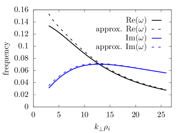
Figure 1: Comparison of exact (solid lines) and approximate analytical (dashed lines) growth rates for the case $\tau=1$ and $m_{i}/m_{e}=337824$ (tungsten ions).

Eq. (33) indicates that for $k_{\parallel}>0$ there is an instability with peak growth rate $\gamma$ at wavelengths $\mathbf{k}_{m}$ satisfying $(\partial\gamma/\partial k_{\parallel})|_{\mathbf{k}_{m}}=(\partial\gamma/\partial k_{\perp})|_{\mathbf{k}_{m}}=0$. These constraints give

$$\frac{2}{\sqrt{\upi}}k_{\parallel,m}|L_{n}|\left(1+\tau+k_{\perp,m}^{2}\lambda_{e}^{2}\right)=k_{\perp,m}\rho_{e},$$ (34)

with the largest growth rate for $k_{\perp,m}\lambda_{e}=0$. Using these results in Eq. (33) gives

$$\omega_{m}=\frac{\tau}{4\sqrt{\upi}\left(1+\tau\right)}\frac{v_{\mathrm{th},i}}{|L_{n}|}\left(\textnormal{i}+\textnormal{sgn}(k_{y}L_{n})\right),$$ (35)

with $\omega_{m}\doteq\omega(\mathbf{k}_{m})$ the complex frequency evaluated at the wavevector $\mathbf{k}_{m}$ that maximizes the linear growth rate.

Plugging Eq. (35) for $\omega_{m}$ into Eq. (20) for turbulent heating and using the appropriate approximations for $\Upsilon(k_{y}\rho_{s})$ and $Z(\zeta_{s})$ gives

$$\begin{split}\hat{H}_{\mathbf{k},i}=-\hat{H}_{\mathbf{k},e}&\approx\frac{k_{y}\rho_{e}}{k_{\parallel}v_{\mathrm{th},i}}\textnormal{Re}\left(\omega\right)\frac{|L_{n}|}{L_{n}}\frac{\sqrt{\upi}}{4}\\ &=\frac{\tau}{8\sqrt{\upi}}>0.\end{split}$$ (36)

So ions are heated and electrons are cooled; i.e., the instability acts to equalize $v_{\mathrm{th},e}$ and $v_{\mathrm{th},i}$ and thus stabilize the mode.

4 Simulation results

We now provide numerical data to verify our analytical predictions. All simulations were conducted using the local, Eulerian gyrokinetic code GS2 (Kotschenreuther et al., 1995; Dorland et al., 2000) with kinetic electrons and a single ion species immersed in a straight, uniform magnetic field and with a cross-field density gradient. The fluctuations are constrained to be purely electrostatic, and we take $k_{\perp}\lambda_{e}=0$. Each simulation used 32 points along the magnetic field direction ($z$), and the velocity space is sampled on a polar grid (Barnes et al., 2010), with 12 points in speed $v$ and 16 points in pitch angle $v_{\parallel}/v$.

First we consider the case of an electron-positron plasma. The linear growth rates, maximized over $k_{\parallel}$ and $k_{\perp}$, are plotted against $T_{e}/T_{i}$ in Fig. (2). They are normalized by $|L_{n}|/v_{0}$, with $v_{0}\doteq\sqrt{v_{\mathrm{th},i}v_{\mathrm{th},e}}$, in order to make manifest the expected symmetry of the growth rates with respect to the interchange of $T_{i}$ and $T_{e}$. As predicted, the plasma is stable only when $T_{e}=T_{i}$, and the growth rates are symmetric about $T_{e}/T_{i}=1$.

Also shown in Fig. (2) are the quasilinear heating estimates defined in Eq. (20) and the heating determined from nonlinear simulations as a function of $T_{e}/T_{i}$. The nonlinear simulations employed 47 modes (after de-aliasing) in both directions perpendicular to the magnetic field ($x$ and $y$). As we showed analytically, the heating (both quasilinear and nonlinear) is antisymmetric about $T_{e}/T_{i}=1$, with the heating acting to equilibrate the electron and positron temperatures and thus shut off the linear instability.

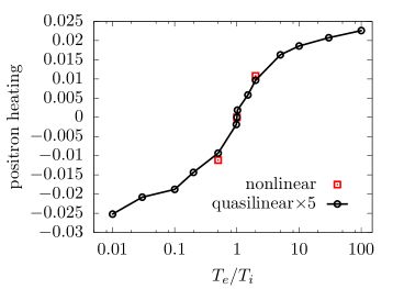
Figure 2: Normalized linear growth rates maximized over $k_{\parallel}$ and $k_{y}$ (left) and corresponding turbulent heating (right) from GS2 simulations as a function of electron-ion temperature ratio for an electron-positron plasma. The quasilinear turbulent ion heating $\hat{H}_{i}$ (black circles and line) given by Eq. (20) is weighted by the linear growth rate $\gamma|L_{n}|/v_{0}$ to qualitatively estimate saturated fluctuation amplitudes. The turbulent ion heating $(H_{i}|L_{n}|/nT_{0}v_{0})(|L_{n}|/\rho_{0})^{2}$ obtained from nonlinear simulations is also given (red squares). Here $\rho_{0}=v_{0}/\Omega_{i}$, with $v_{0}$ the geometric mean of the ion and electron thermal speeds.

We next show the growth rates and turbulent ion heating as a function of electron-ion temperature for an electron-proton plasma in Fig. (3). Again we see that the plasma is unstable for $v_{\mathrm{th},e}\neq v_{\mathrm{th},i}$. Furthermore, the ion turbulent heating is positive definite for $v_{\mathrm{th},e}>v_{\mathrm{th},i}$, in agreement with our approximate analytic result.

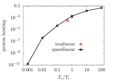
Figure 3: Normalized linear growth rates maximized over $k_{\parallel}$ and $k_{y}$ (left) and corresponding turbulent heating (right) from GS2 simulations as a function of electron-ion temperature ratio for an electron-proton plasma. The quasilinear turbulent ion heating $\hat{H}_{i}$ (black circles and line) given by Eq. (20) is weighted by the linear growth rate $\gamma|L_{n}|/v_{\mathrm{th},i}$ to qualitatively estimate saturated fluctuation amplitudes. The turbulent ion heating $(H_{i}|L_{n}|/nT_{i}v_{\mathrm{th},i})(|L_{n}|/\rho_{i})^{2}$ obtained from nonlinear simulations is also given (red squares)

5 Conclusions

The analytical and numerical results shown in this paper indicate that turbulent heating driven by the electron drift wave instability present in an inhomogeneous, magnetized plasma acts to stabilize the mode. Stabilization occurs when the ion and electron thermal speeds are equal. For a conventional mass ratio plasma with $T_{i}\sim T_{e}$, this leads to the ions being heated and the electrons cooled; for a pair plasma, the turbulent heating acts to equalize the ion and electron temperatures.

While turbulent heating acts to stabilize the mode, it is not the only stabilization mechanism in the system. We showed that the instability drives particle transport that flattens the driving density gradient on a time scale at least as fast as the heating influences the electron-ion temperature ratio. Consequently, for the turbulent heating to fully set the thermal equilibrium there must be additional physics that fixes the density gradient; e.g., an external density source or a lowest order equilibrium set by gravitational forces. In this case, thermal equilibrium would correspond to $T_{i}/T_{e}=\sqrt{m_{i}/m_{e}}$.

The authors would like to thank F. I. Parra, A. A. Schekochihin and A. Zocco for useful discussions. M. Barnes was supported in part by STFC grant ST/N000919/1. The authors also acknowledge the use of ARCHER through the Plasma HEC Consortium EPRSC grant number EP/L000237/1 under project e281-gs2 and the use of the EUROfusion High Performance Computer (Marconi-Fusion) under project MULTEI.

References

• Barnes et al. (2010) Barnes, M., Dorland, W. & Tatsuno, T. 2010 Velocity space resolution in gyrokinetic simulations. Phys. Plasmas 17, 032106.
• Barnes et al. (2012) Barnes, M., Parra, F. I. & Dorland, W. 2012 Turbulent transport and heating of trace heavy ions in hot, magnetized plasmas. Phys. Rev. Lett. 109, 185003, arxiv:1207.5175.
• Candy (2013) Candy, J. 2013 Turbulent energy exchange: Calculation and relevance for profile prediction. Phys. Plasmas 20, 082503.
• Chandran et al. (2010) Chandran, B. D. G., Li, B., Rogers, B. N., Quataert, E. & Germaschewski, K. 2010 Perpendicular ion heating by low-frequency alfven-wave turbulence in the solar wind. Astrophys. J. 720, 503.
• Collier et al. (1996) Collier, M. R., Hamilton, D. C., Gloeckler, G., Bochsler, P. & Sheldon, R. B. 1996 Neon-20, oxygen-16, and helium-4 densities, temperatures, and suprathermal tails in the solar wind determined with wind/mass. Geophys. Res. Lett. 23, 1191.
• Cranmer et al. (1999) Cranmer, S. R., Field, G. B. & Kohl, J. L. 1999 Spectroscopic constraints on models of ion cyclotron resonance heating in the polar solar corona and high-speed solar wind. Astrophys. J. 518, 937.
• Dorland et al. (2000) Dorland, W., Jenko, F., Kotschenreuther, M. & Rogers, B. N. 2000 Electron temperature gradient turbulence. Phys. Rev. Lett 85, 5579.
• Galeev et al. (1963) Galeev, A. A., Oraevsky, V. N. & Sagdeev, R. Z. 1963 ”universal” instability of an inhomogeneous plasma in a magnetic field. J. Exptl. Theoret. Phys. 44, 903.
• Helander (2014) Helander, P. 2014 Microstability of magnetically confined electron-positron plasmas. Phys. Rev. Lett. 113, 135003.
• Helander & Plunk (2015) Helander, P. & Plunk, G. G. 2015 The universal instability in general geometry. Phys. Plasmas 22, 090706.
• Howes et al. (2008) Howes, G. G., Cowley, S. C., Dorland, W., Hammett, G. W., Quataert, E. & Schekochihin, A. A. 2008 A model of turbulence in magnetized plasmas: Implications for the dissipation range in the solar wind. J. Geophys. Res. 113, A05103.
• Kohl et al. (1997) Kohl, J. L., Noci, G., Antonucci, E., Tondello, G., Huber, M. C. E., Gardner, L. D., Nicolosi, P., Strachan, L., Fineschi, S., Raymond, J. C., Romoli, M., Spadaro, D., Panasyuk, A., Siegmund, O. H. W., Benna, C., Ciaravella, A., Cranmer, S. R., Giordano, S., Karovska, M., Martin, R., Michels, J., Modigliani, A., Naletto, G., Pernechele, C., Poletto, G. & Smith, P. L. 1997 First results from the soho ultraviolet coronograph spectrometer. Solar Physics 175, 613.
• Kotschenreuther et al. (1995) Kotschenreuther, M., Rewoldt, G. & Tang, W. M. 1995 Comparison of initial value and eigenvalue codes for kinetic toroidal plasma instabilities. Comp. Phys. Comm. 88, 128–140.
• Krall & Rosenbluth (1965) Krall, N. A. & Rosenbluth, M. N. 1965 Universal instability in complex field geometries. Phys. Fluids 8, 1488.
• Landreman et al. (2015) Landreman, M., T. M. Antonsen, Jr. & Dorland, W. 2015 Universal instability for wavelengths below the ion larmor scale. Phys. Rev. Lett. 114, 095003.
• Pedersen & Boozer (2002) Pedersen, T. Sunn & Boozer, A. H. 2002 Confinement of nonneutral plasmas on magnetic surfaces. Phys. Rev. Lett. 88, 205002.
• Quataert & Gruzinov (1999) Quataert, E. & Gruzinov, A. 1999 Turbulence and particle heating in advection-dominated accretion flows. Astrophys. J. 520, 248.
• Schmidt et al. (1980) Schmidt, W. K. H., Rosenbauer, H., Shelly, E. G. & Geiss, J. 1980 On temperature and speed of he++ and o6+ ions in the solar wind. Geophys. Res. Lett. 7, 697.