Optical Follow-up of Planck Cluster Candidates with Small Instruments

Abstract

We report on the search for optical counterparts of Planck Sunyaev-Zel’dovich (SZ) cluster candidates using a $0.6\,\mathrm{m}$ non-professional telescope. Among the observed sources, an unconfirmed candidate, PSZ2 G156.24+22.32, is found to be associated with a region of more than $100$ galaxies within a $3$ arcminutes radius around the Sunyaev-Zel’dovich maximum signal coordinates. Using $14$ hours of cumulated exposure over the Sloan color filters $g^{\prime}$, $r^{\prime}$, $i^{\prime}$, and $z^{\prime}$, we estimate the photometric redshift of these galaxies at $z_{\mathrm{phot}}=0.29\pm 0.08$. Using the red-sequence galaxy method gives a photometric redshift of $0.30{\,}^{+0.03}_{-0.05}$. Combined with the Planck SZ proxy mass function, this would favor a cluster of $4.4\times 10^{14}$ solar masses. This result suggests that a dedicated pool of observatories equipped with such instruments could collectively contribute to optical follow-up programs of massive cluster candidates at moderate redshifts.

1 Introduction

Among the foregrounds imprinting temperature anisotropies and spectral distortions on the Cosmic Microwave Background (CMB) radiation, the thermal Sunyaev-Zel’dovich effect is of particular interest for Astrophysics and Cosmology (Sunyaev & Zeldovich, 1970, 1972, 1980; Sazonov & Sunyaev, 1999; Challinor et al., 2000; Bunn, 2006). Inverse Compton scattering of the CMB photons by the hot electrons present within galaxy clusters results in a shift and distortion of their blackbody spectrum towards higher frequencies. The intracluster plasma cools down the CMB radiation at frequencies typically lower than $217\,\mathrm{GHz}$ while warming it up at higher frequencies. Such a signature is unique among foregrounds and has been intensively used by the Planck satellite collaboration and other CMB ground telescopes, such as the Atacama Cosmology Telescope (ACT) and the South Pole Telescope, to provide unprecedented catalogues of Sunyaev-Zel’dovich (SZ) sources (Hasselfield et al., 2013; Planck Collaboration et al., 2014a; Bleem et al., 2015; Planck Collaboration et al., 2015a). The SZ effect does not depend on the redshift, and therefore provides a new high-redshift observable of galaxy clusters. The full sky coverage of the Planck satellite has allowed the release of the PSZ2 catalog in Planck Collaboration et al. (2016a) containing more than $1600$ SZ sources. Among them, $1200$ objects have been confirmed as clusters by the Planck collaboration through their cross identification in the Meta-Catalog of X-ray detected clusters (MCXC) (Piffaretti et al., 2011), with optical counterparts in the Sloan Digital Sky Survey (SDSS) (York et al., 2000), in the redMaPPer catalog (Rozo et al., 2015; Rykoff et al., 2016), in the Nasa/IPAC Extragalactic Database (NED), and with infrared galaxy overdensities in the Wide-field Infrared Survey (WISE) (Wright et al., 2010). More than $400$ SZ sources were still unconfirmed at the time of publication of the catalog and not all confirmed sources have redshift information. Cluster counts using the PSZ2 catalogue have been used for Cosmology in Planck Collaboration et al. (2016b). They allow CMB-independent estimations of the amplitude of the matter power spectrum $\sigma_{8}$ and of the matter density parameter $\Omega_{\mathrm{m}}$, which are currently in mild tension with the best fit $\Lambda$CDM model obtained from CMB primary anistropies alone (Planck Collaboration et al., 2016c). Doing cosmology with cluster counts requires the determination of a scaling relation between the total integrated Compton parameter $Y_{\mathrm{5R500}}$, the cluster angular size, $\theta_{\mathrm{s}}$, and its total mass, $M_{500}$, (defined over a radius enclosing $500$ times the critical density at redshift $z$). As explained in Planck Collaboration et al. (2014b), SZ measurements give information on the relation between $Y_{\mathrm{5R500}}$ and $\theta_{\mathrm{s}}$ while breaking the degeneracy between $Y_{\mathrm{5R500}}$ and $M_{500}$, at a given redshift $z$, relies on a scaling relation extracted from X-ray observations and assuming hydrostatic equilibrium of the intracluster gas (Arnaud et al., 2010, 2007). For each of the SZ sources, the PSZ2 catalog provides the most probable hydrostatic mass $M_{\mathrm{SZ}}(z)$ (and its standard deviation) assuming the scaling relation to hold. Follow-up programs of SZ sources are therefore of immediate interest in evaluating $M_{\mathrm{SZ}}$ for a given cluster by the determination of its redshift $z$.

Dedicated optical follow-up programs of unconfirmed Planck clusters have been carried on using professional telescopes since the publication of the PSZ2 catalog. The Pan-STARRS $1.8\,\mathrm{m}$ telescope survey (Liu et al., 2015) has provided $60$ confirmations combined with spectroscopic redshift measurements. Another $16$ high-redshift clusters have been confirmed by the Canada-France-Hawaï telescope (CFHT) with photometric redshifts together with richness mass estimates (van der Burg et al., 2016). Spectroscopic redshifts and confirmation of $13$ more clusters have been provided by the $1.5\,\mathrm{m}$ Russian-Turkish telescope, the $2.2\,\mathrm{m}$ Calar Alto Observatory telescope, and the $6\,\mathrm{m}$ Bolshoi (BTA) telescope in Vorobyev et al. (2016) (see also Planck Collaboration et al., 2015b). The Planck collaboration has used a month of observations at the Canary Islands Observatories for the confirmation of $73$ more candidates (Planck Collaboration et al., 2016d). Although these numbers could suggest that unconfirmed SZ sources would soon be exhausted, artificial neural networks have recently been used on the Planck CMB measurements to improve the detection threshold of SZ sources. A new catalog discussed by Hurier et al. (2017) contains almost $4000$ galaxy cluster candidates. In addition, ground-based telescopes are still contributing to new SZ detection thereby calling for an increase of the telescope time needed for follow-up programs (Hilton et al., 2017) .

In this paper, we explore and report on the possibility to use sub-meter non-professional telescopes (of typically $0.5\,\mathrm{m}$-$0.6\,\mathrm{m}$ diameter) to carry on optical follow-up searches of unconfirmed SZ sources. In spite of obvious technical challenges, some scientific measurements can be achieved such as galaxy counts and photometric redshift estimates. As a test case, we report on a cluster candidate, PSZ2 G156.24+22.32, which has not been confirmed in any of the aforementioned catalogs, nor in the follow-up programs, and which is not included in the SDSS sky coverage (Ahn et al., 2012; Wen et al., 2012).

The paper is organized as follows. Section 2 describes the observations and the method used for data reduction. Some details are provided concerning the observatory, the hardware used, as well as the technical difficulties overcome for achieving sufficiently good tracking and imaging for photometry. In Sect. 3, we present our main results, namely galaxy counts, photometric redshift, and optical richness estimates for PSZ2 G156.24+22.32. In Sect. 4, various tests to assess the validity of our measurements are presented. In the conclusion, we briefly discuss a proof of concept on what small telescopes can and cannot achieve, would they massively contribute to the search of optical counterparts of SZ sources.

2 Observations and data reduction

2.1 Observatory and instrumentation

The observatory of Saint-Véran is located in France, at $44\degree 42\arcmin 03\arcsec$ N, $6\degree 52\arcmin 06\arcsec$ E, at an altitude of $2930\,\mathrm{m}$ a.s.l. (IAU code 615). It has been managed by the Astroqueyras Association for roughly $30$ years, and is intended to allow amateur astronomers to observe under better conditions compared to that of typical lower altitude suburban skies.

The observatory comprises three main instruments: a Cassegrain telescope with a diameter of $0.62\,\mathrm{m}$ and $9\,\mathrm{m}$ of focal length (T62), and two Ritchey-Chrétien telescopes, each having a diameter of $0.5\,\mathrm{m}$ and $4\,\mathrm{m}$ of focal length. The instrument mainly used in the context of this work is the T62. Although the primary mirror is of $0.62\,\mathrm{m}$ diameter, the holding baffle reduces the effective aperture to $0.60\,\mathrm{m}$. The T62 is mounted on a German-type Reosc equatorial mount, equipped electronically for semi-automatic target pointing. The imaging device used is an Apogee U16M CCD camera equipped with a KAF-16803 sensor, cooled at $-20\degree\,\mathrm{C}$. The sensor has $4096\times 4096$ pixels of area $9\times 9\,\micron^{2}$, which implies a genuine angular sampling of $0.21\arcsec\times 0.21\arcsec$. The field of view is a square of $14\arcmin$ side.

The King (1989) polar drift method has been applied to align the mount right ascension (R.A.) and Earth rotation axes, and therefore improves the pointing and tracking accuracy. This operation must be done regularly, due to local seismic activity and a slow rotation of the mountain where the observatory is installed. In the context of this work, the residual angle between the right ascension axis of the mount and the Earth rotation axis was reduced to a value smaller than roughly $10\arcsec$. The native periodical error of the RA movement is estimated to be around $5\arcsec$ at vanishing declination (DEC), with smooth amplitude variations during tracking. The tracking accuracy is yet improved by auto-guiding the T62, i.e., by correcting any deviations between the sky and mount movements. This is achieved using a second camera installed on a $0.2\,\mathrm{m}$ Schmidt-Cassegrain telescope. It is mounted in parallel with the T62 and has a focal length of $2\,\mathrm{m}$. The camera has a Exview sensor made of $752\times 580$ pixels of area $8.2\times 8.4\,\micron^{2}$. This allows for exposures up to $10$ to $15$ minutes long, depending on the telescope orientation and the target declination. The resulting guiding error is estimated from the average point spread function of the stars and found to be less or equal to the seeing. The measured full width at half maximum (FWHM) varies between $1.2\arcsec$ to $2\arcsec$ across the exposure series. These FWHM values led us to optimize the sampling for the Apogee U16M camera. A binning grouping four pixels into one has been used, yielding an angular sampling of $0.42\arcsec\times 0.42\arcsec$.

The search for optical counterparts of the SZ targets has been performed in luminance, i.e. without a specific spectral filtering of the light input. Once the galaxies have been located, color imaging of the suspected cluster is done using interferential filters. For this work, we have used a set of Astrodon Gen 2 Sloan photometric filters corresponding to the SDSS photometric standards (Fukugita et al., 1996; Smith et al., 2002). The low quantum efficiency of the KAF-16803 sensor in the ultraviolet wavelength range led us to consider only the $g^{\prime}$, $r^{\prime}$, $i^{\prime}$, and $z^{\prime}$ filters.

2.2 Data acquisition

The search of optical counterparts of the Planck SZ candidates took place during two one-week long observation missions, one from 2015 November 7 to November 15, and the other between 2017 February 18 and February 26.

The goal of the first mission was to assess the feasibility of the project and was dedicated to the observations of confirmed Planck clusters having known redshifts. Individual galaxy identifications for five clusters having redshifts ranging from $0.1$ to $0.6$ were successfully performed. In particular, color imaging of two of them, PSZ2 G138.32-39.82 and PSZ2 G164.18-38.88, located at redshift $0.280$ and $0.08$, respectively, allowed us to test the instrumentation for photometric redshift estimation. A low-signal test of our apparatus was achieved by successfully resolving individual galaxies in luminance within a distant cluster PSZ2 G144.83+25.11, having a redshift of $0.584$ (also known as MACS J0647.7+7015). These results are discussed in more details in Sect. 4.

The 2017 winter mission was dedicated to the search of non-confirmed Planck SZ sources optical counterparts. Five objects from the PSZ2 catalog, having no X-ray nor optical counterparts, have been pointed. The choice of the targets has been made taking into account several constraints. First, we have kept the airmass reasonably close to unity and only objects well-above the horizon, by at least $40\degree$, have been considered. Second, the targets should not be too close from the Milky Way to minimize possible confusion between faint stars and distant galaxies.

A technical difficulty associated with the use of a small telescope is the exposure time needed to collect enough photons for galaxy detection. Based on empirical results from the first mission, around $1$ hour of exposure has been accumulated per target, made from $10$ minutes luminance slices. After performing some minimal data reduction, a visual inspection allowed us to check for overdensity within the $14\arcmin$ field of view around the SZ signal coordinates.

Among the observed targets, PSZ2 G156.24+22.32 located in the Lynx constellation (northern celestial hemisphere), ended up showing a significant object count. We therefore started data acquisition in the color filter $g^{\prime}$, $r^{\prime}$, $i^{\prime}$ and $z^{\prime}$ from 2017 February 21 until the end of the mission on February 26. According to the above-mentioned criteria, PSZ2 G156.24+22.32 was of sufficiently high altitude in the sky only during the second half of the night. The first part of the night was therefore dedicated in the color imaging of our reference photometric SDSS DR9 galaxy field, located nearby M63, which is roughly at the same altitude in the sky than the one occupied by the cluster later on. Around $1.5$ hours of cumulated exposure per filter were taken for the reference field. In total, around $14$ hours of color exposure have been used to derive the results presented below.

2.3 Reduction

In order to produce photometric usable data, image reduction has been performed in two steps.

In a first pass, we have used the Image Reduction and Analysis Facility (IRAF) to correct each image from bias, dark currents and nonlinear response pixels (Tody, 1986, 1993). Basic astrometric registration and airmass calculations are also performed for each color images in order to provide a World Coordinate System (WCS) compatible header for each of them.

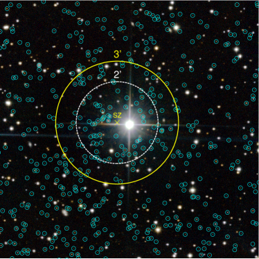
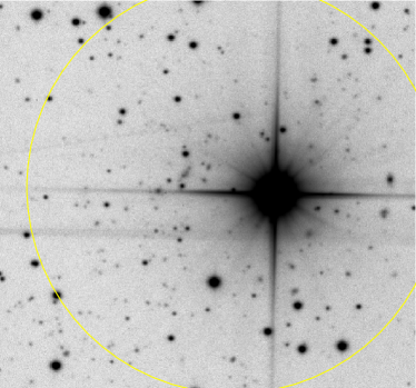
Figure 1: Upper panel: circular regions of radius $2\arcmin$ and $3\arcmin$ centered at the Planck SZ maximum signal location (marked by a cross) used for galaxy counts and photometric redshift estimates. Objects with a small circle are matched sources across the color filters (stars excluded; see the text). The lower panel is a zoom within the $3\arcmin$ region.

The second pass consists in an accurate astrometry and photometry solving starting from the WCS single-epoch images produced by the first pass. For this purpose, we have used the AstrOmatic software suite (Bertin & Arnouts, 1996; Bertin, 2006; Bertin et al., 2002). Sources are extracted in all images using SExtractor (version 2.19.5) with a detection and analysis threshold set at $1.5\sigma$ with respect to the local background noise. An astrometric and photometric solution is then obtained by using the Scamp code. It has been run in multi-instruments mode, one astrometric and photometric instrument for each color filter, plus luminance, and we have allowed for astrometric distortions within a given instrument. The reference astrometry catalog chosen is the USNO-B1 (Monet et al., 2003). The reported internal astrometric errors are small, $0.05\arcsec$ (FWHM), and remain negligible with respect to the ones of the reference catalog, evaluated at $0.5\arcsec$ (FWHM). However, a shear contraction amplitude of typically $0.15\%$ has been corrected for each instrument, far above what one could have expected for an airmass never exceeding $1.4$ ($0.05\%$). The distortion map of the pixel scale computed by Scamp indeed reveals an almost constant hyperbolic pattern over all filters and luminance. Although the reason for this distortion is unclear, different sources are possible, among which a stress on the primary mirror, or still a minor mirror alignment issue leading to astigmatism appearing at moderate defocus. Time constraint did not allow for a deeper exploration and resolution of this issue. Concerning the photometric solution, zero-point changes across the exposure series have been corrected within each filter. The standard deviations of these corrections are found in the following ranges: $\Delta g^{\prime}_{0}\in[0.1,0.4]$, $\Delta r^{\prime}_{0}\in[0.05,0.3]$, $\Delta i^{\prime}_{0}\in[0.05,0.4]$ and $\Delta z^{\prime}_{0}\in[0.05,0.5]$. The first (and lowest) value is for high signal-over-noise matched sources only while the second one includes all matched objects between the single-epoch images and the reference catalog. Although corrected, these numbers show some degradation of our photometric stability up to half a magnitude for faint objects in the $z^{\prime}$ filter, and some significant scatter in the $g^{\prime}$ band as well. This could be attributed to the parasitic presence of a $V=7.2$ magnitude double star in the field of view as a much lower scatter is obtained for the SDSS reference field (see below and Fig. 1).

In the last step, coaddition of the corrected single-epoch images for each filter (and luminance) has been delegated to the SWarp code, which takes care of background estimation, as well as resampling, for each image. Highest contrasts have been obtained by using a median weighted stacking, the weights being estimated from the background noise (see Bertin et al., 2002).

2.4 Calibration

The absolute zero-point magnitudes for the four coadded images in the $g^{\prime}$, $r^{\prime}$, $i^{\prime}$, and $z^{\prime}$ filter have been determined from our SDSS DR9 reference galaxy field (see Sect. 2.2).

The reference images have been reduced and flattened, for each color filter, exactly as described above. Then, we have used the SExtractor code over the coadded images to create a catalog of photometric reference sources. The magnitude measurement method chosen is mag_auto and only high signal-over-noise detections have been kept, $5\sigma$ above the estimated background (Bertin & Arnouts, 1996). Our reference catalogs, in $g^{\prime}$, $r^{\prime}$, $i^{\prime}$, and $z^{\prime}$, are then matched together and to the SDSS DR9 catalog by cross identifying objects of same position at less than $1\arcsec$. For this purpose, the imaging software DS9 has been used to create a set of roughly $30$ galaxies for which one has both the non-calibrated mag_auto magnitudes and the modelMag magnitudes as provided by the SDSS DR9 catalog (Ahn et al., 2012). The zero-point values for each filter, $g^{\prime}$, $r^{\prime}$, $i^{\prime}$ and $z^{\prime}$, have been determined with IRAF using a photometric weighting based on the magnitude error estimates made by SExtractor.

In the following, unless specified otherwise, our calibrated mag_auto magnitudes will be referred to as $griz$ since they are indistinguishable of the modelMag SDSS DR9 magnitudes within the uncertainties of our apparatus and methodology.

3 Results

3.1 Color catalog of matched objects

From the photometric usable images obtained as described in Sect. 2, we have constructed a $griz$ catalog of all objects suspected to be galaxies within the $14\arcmin$ field of view around the SZ coordinates associated with PSZ2 G156.24+22.32.

Again, the SExtractor code has been used for this purpose, in single-image mode and with a detection threshold at $2\sigma$ for the $g^{\prime}$, $r^{\prime}$, and $i^{\prime}$ filter. As discussed in the previous section, the $z^{\prime}$ image showing higher noise than the others, SExtractor has been used in two-images mode, $2\sigma$ detection coming from the $i^{\prime}$ image, photometry coming from the $z^{\prime}$ one with an analysis threshold set at $1.5\sigma$. Separation between stars and galaxies is made using the neural network classifier of SExtractor by discarding all objects having a CLASS_STAR greater than $0.98$. The remaining objects over all filters are then matched together according to their position, required to be the same at $1\arcsec$, and then rejected if they correspond to an optical counterpart in the USNO-URAT1 catalog (Zacharias et al., 2015).

In Fig. 1, the SZ signal center, as reported in the PSZ2 catalog, has been represented by a cross and small circles have been drawn around all the remaining objects of our $griz$ catalog. A visual inspection of their shape suggests that many of them should be galaxies while some overdensity is visible left from the SZ center. Let us notice that having chosen to exclude objects from the USNO-URAT1 catalog is unexpectedly doing a good job in removing bright and close galaxies visible in the picture. A closer look to Fig. 1 also reveals that many small objects close to the bright star, and which are certainly galaxies belonging to the cluster, are not present in our $griz$ catalog. This is due to the fact that these sources have been excluded by SExtractor as being too much contaminated, in at least one color, by the parasitic glow of the star. As discussed below, five more objects close to the star end up being obvious outliers and will be removed from the subsequent analysis (drawn with a small white box).

From the Planck catalog MMF3, we have extracted the two-dimensional probability distribution in the plane $(Y_{\mathrm{5R500}},\theta_{\mathrm{s}})$ associated with PSZ2 G156.24+22.32 (Planck Collaboration et al., 2016a). By marginalizing over the integrated Comptonization parameter $Y_{\mathrm{5R500}}$, the most probable angular size of the SZ region is found to be

$$\theta_{\mathrm{s}}=2.5\arcmin\pm 0.5\arcmin,$$ (1)

at $68\%$ of confidence. As a result, we have defined a circular region around the SZ maximum having a radius of $3\arcmin$ to encompass the whole SZ region. It is represented as the yellow circle in Fig. 1. To assess the sensitivity of the results with respect to the chosen cluster angular size, another circular region has been defined, centered at the SZ location, with a radius of $2\arcmin$ (dashed inner circle in Fig. 1). The intersection of our catalog with these two regions will be referred to as $griz_{3}$ and $griz_{2}$ in the following; they contain $114$ and $58$ objects, respectively (including the five outliers; see Fig. 1).

Finally, let us mention that PSZ2 G156.24+22.32 is associated in the PSZ2 catalog with a value of $\texttt{Q\_NEURAL}=0.96$, which indicates a high probability of being a genuine SZ source. Moreover, as reported by van der Burg et al. (2016), all the SZ candidates validated by optical counterparts in this work have a $\texttt{Q\_NEURAL}>0.8$, thereby rendering our observation of galaxy overdensity around the SZ location not unlikely.

3.2 Photometric redshift and cluster mass

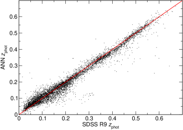
Figure 2: Photometric redshift estimates of the artificial neural network over an independent testing set of $250\,000$ galaxies from the SDSS DR9 catalog. The upper panel shows the neural net estimated redshift $z_{\mathrm{phot}}$ as a function of photometric SDSS redshift (the plot has been truncated to $8000$ random samples for illustration convenience). The lower panel shows the distribution of the residuals $\Delta z_{\mathrm{phot}}$ and has a standard deviation of $\sigma_{\Delta z_{\mathrm{phot}}}=0.027$.

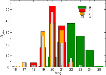
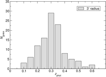
Figure 3: Upper panel: magnitude distribution in $griz$ for the $109$ galaxies observed within the $3\arcmin$ radius region centered at the SZ coordinates. The lower panel is the corresponding photometric redshift distribution as inferred by our neural network trained over the SDSS DR9 catalog (five outliers having negative redshifts removed).

In order to evaluate the photometric redshift of the objects belonging to our color catalogs, we have used an artificial neural network (ANN) regression of the SDSS DR9 color-redshift relationship, but only for the reduced set of $griz$ colors. For this purpose, the publicly available SkyNet code has been run to train a simple feed-forward artificial neural network (Graff et al., 2012, 2014; Hobson et al., 2014). The ANN input layer takes as argument the $griz$ modelMag magnitudes, and the output layer returns the photometric redshift. All input and hidden layer nodes of the ANN are evaluating the hyperbolic tangent of the biased weighted addition of the input signals. For faster training, the output layer has, however, been chosen to only perform a biased linear combination of the last hidden layer nodes. The training set chosen consists of $250\,000$ photometric clean objects from the SDSS DR9 data release, selected to have nearest neighbors in the SDSS color space, photometric redshift errors not exceeding $0.03$, and color magnitudes in the range $[12,29]$. Another group of $250\,000$ objects, selected with the same criteria, has been used as a testing set to check the quality of the ANN regression. We have found that a good enough learning of the ANN over the training set requires four hidden layers of $90$ nodes each, in addition to the input layer of four nodes and the single-node output layer. In total, SkyNet has been used to find the optimal values of more than $30\,000$ weights and biases as described in Graff et al. (2014).

The upper panel of Fig. 2 shows the ANN output values obtained by inputting the $griz$ color magnitudes of the SDSS DR9 testing set as a function of the photometric redshift estimated by the SDSS DR9 collaboration. The lower panel shows the distribution of the residuals. The ANN reproduces very well the SDSS estimated photometric redshifts for almost all values from $z_{\mathrm{phot}}\simeq 0$ to $z_{\mathrm{phot}}\simeq 0.8$. The standard deviation of the residuals, over a quarter million of objects, reads $\sigma_{\Delta z_{\mathrm{phot}}}=0.027$. Because it is of the same order as the SDSS photometric redshift errors of the training catalog, the ANN regression is nearly optimal.

Applying the trained ANN over the color magnitudes of our $griz_{3}$ catalog gives the distribution of photometric redshifts of all galaxies located at less than $3\arcmin$ from the SZ center associated with PSZ2 G156.24+22.32. In total, $griz_{3}$ contains $114$ objects, five of them end up having a negative photometric redshift. A closer examination of these outliers show that they have unusually large values for the estimated error on mag_auto ($\Delta m\gtrsim 0.2$), and they are all located close to the bright star. They have therefore been removed from the analysis and are represented as white boxes in Fig. 1. The photometric redshift distribution of all the $109$ remaining objects has been plotted in the lower panel of Fig. 3 while the upper panel shows their color magnitude distribution. A clear reddening of the objects can be observed between the $g$ and $r$ magnitude, and to a lesser extend between $r$ and $i$ as well, supporting the claim that the sources are redshifted galaxies. The photometric redshift distribution indeed shows a peak around a redshift of $0.3$ and no object are found with a redshift less than $0.08$ (up to the five outliers). In order to estimate the mode of the redshift distribution, the “ash” package of the R-project software suite has been used to compute a polynomial density estimate and extract its maximum. One finds

$$z_{\mathrm{phot}}=0.29\pm 0.08.$$ (2)

To minimize sensitivity to potential systematics, the quoted error stands for the median absolute deviation around the mode, normalized such that it would match the usual standard deviation for a Gaussian distribution. Changing the smoothing kernel does not affect the estimation of the mode by more than $0.01$. As expected, the median absolute deviation is larger than the intrinsic ANN residuals plotted in Fig. 2 due to the color-magnitude errors of our measurements.

The most probable hydrostatic mass, $M_{\mathrm{SZ}}(z)$, as well as its standard deviation, as a function of the cluster redshift $z$ is given by the Planck collaboration in the MMF3 catalog (Planck Collaboration et al., 2016a). Combined with Eq. (2), it yields

$$M_{\mathrm{SZ}}=\left(4.4\pm 1.3\right)\times 10^{14}M_{\sun}.$$ (3)

The quoted errors are the intersect of the median absolute deviations associated with the photometric redshift and the standard deviation on $M_{\mathrm{SZ}}(z)$.

In order to test the robustness of Eq. (2) with respect to the chosen condition under which galaxies belong to the cluster, we have also considered a region of $2\arcmin$ radius around the SZ coordinates. This corresponds to the lower $1\sigma$ limit of $\theta_{\mathrm{s}}$ in Eq. (1), and to the objects constituting the $griz_{2}$ color catalog. After the removal of the same five outliers as in the $griz_{3}$ catalog, it remains $53$ galaxies for which one finds $z_{\mathrm{phot}}=0.29\pm 0.11$. As before, the first value is the mode and the error stands for the median absolute deviation around the mode.

3.3 Optical richness

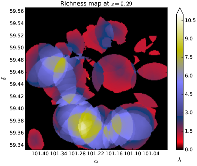
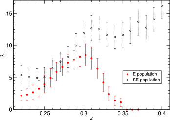
Figure 4: Upper panel: map of the optical richness $\lambda$ over the field of view of figure 1 (the red sequence galaxies are assumed to be at $z=0.29$). The lower panel shows the dependence of $\lambda(z)$ for the two locations exhibiting maximal richness in the upper panel. Only the one located East to the SZ center is well bounded in redshift and can be associated with a galaxy cluster (red points).

A visual inspection of the red luminous objects contiguous to the ones contained within the $2\arcmin$- and $3\arcmin$-radius regions suggests that a galaxy population is also present further southest (SE), i.e., toward the lower left corner of Fig. 1. Let us notice that the NED database reports one X-ray source in this region, 1RXS J064506.9+592603 (Voges et al., 1999).

To quantify which objects are clustered, we have estimated the optical richness, $\lambda$, as discussed in Rozo et al. (2009). In practice, $\lambda$ has been computed according to the method presented in Rykoff et al. (2012) and Rykoff et al. (2014). In order to use the same luminosity tracer as in these references, we have recalibrated our $i^{\prime}$ filter over the SDSS DR9 reference field by using the $i$ CmodelMag magnitude (instead of the modelMag). The color has been estimated as before, namely our $g-r$ comes from $g^{\prime}$ and $r^{\prime}$ filter calibrated from modelMag magnitudes. This color should be an accurate tracer of the red-sequence galaxies up to redshift $0.35$ (Gladders & Yee, 2000; Koester et al., 2007). All of the magnitudes have been corrected for Galactic extinction and reddening (Schlegel et al., 1998; Schlafly & Finkbeiner, 2011), and the cosmological parameters have been chosen according to the Planck 2015 favored values (Planck Collaboration et al., 2016c).

The presence of the parasiting star and the other uncertainties associated with our small instrumentation are expected to introduce various systematics in the determination of the photometric zero-points. As reported in Rykoff et al. (2012), the determination of $\lambda$ is expected to be accurate for zero-point shifts up to $\pm 0.05$ magnitudes, and we might have systematic uncertainties as large as eight times this value for some objects (see section 2.3). Adding an additional scatter of $0.1$ magnitudes to luminosity and colors is indeed found to increase the value of $\lambda$ by a factor of $2$. As a result, there is a possibility that the following evaluations of $\lambda$ are underestimated, which is inherent to the experimental limitations of our setup. Notice, however, that the dependence of $\lambda$ with respect to the coordinates of the clustering center and to the redshift, remains mostly insensitive to the uncertainties in the photometric zero-points. This is what we focus on in the following.

To minimize the propagation of these potential systematics, we have chosen the radial filter to be

$$R_{\mathrm{c}}(\lambda)=R_{0}\left(\dfrac{\lambda}{100}\right)^{\beta},$$ (4)

with $R_{0}=0.95h^{-1}\,\mathrm{Mpc}$, and $\beta=0.1$ instead of $R_{0}=1h^{-1}\,\mathrm{Mpc}$ and $\beta=0.2$ as done in Rykoff et al. (2012). Our choice is still in the region of minimal intrinsic scatter for red-sequence galaxies, but has the advantage of lowering the impact of underestimated $\lambda$ values. The background galaxies and the red-sequence fit in $g-r$ have been taken as in Rykoff et al. (2012) while the luminosity filter is the one of Rykoff et al. (2014).

The upper panel of figure 4 shows a map of $\lambda$ over the field of view of figure 1, obtained by postulating that the red-sequence galaxies are at the redshift $z=0.29$. The two regions exhibiting maximal richness encompass the one visually expected east from the SZ center (left), around $(\alpha,\delta)=(101.31,59.48)$, and the one associated with the SE population at $(\alpha,\delta)=(101.27,59.36)$ (lower left). In the lower panel of figure 4, we have plotted the optical richness $\lambda(z)$, as a function of the redshift, for these two locations. Only the first one ends up being well localized in redshift space, and this allows us to improve the cluster’s redshift estimate to

$$z_{\lambda}=0.30{\,}^{+0.03}_{-0.05}\,.$$ (5)

The quoted errors are the intercepts for FWHM. As can be seen in figure 4, for the SE population of galaxies, $\lambda(z)$ steadily increases up to $z=0.42$ to vanish at $z=0.7$ (not represented). For these redshifts, the choice of the color filter $g-r$ is no longer accurately tracing red-sequence galaxies, but we can, however, conclude that most of these objects do not belong to the population east from the SZ center.

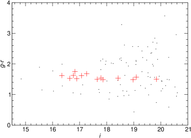
Figure 5: Color-magnitude diagram for the all objects located within a $R_{\mathrm{c}}(\lambda_{\max})\simeq 1.1\,\mathrm{Mpc}$ radius around the cluster center (see the text and Fig. 4). Red crosses are for galaxies identified as cluster members, while the black dots are for all the other objects.

Finally, in figure 5, we have represented the color-magnitude diagram for all objects found within a $R_{\mathrm{c}}(\lambda_{\max})$ radius around the location $(101.31,59.48)$, corresponding to the east population of figure 4. The red crosses represent red-sequence galaxies, which have been identified as belonging to the cluster with a probability greater than $0.5$. The scatter of half a magnitude in $g-r$ for bright objects ($i<17$) might be the result of the aforementioned systematics in the zero-points. As already discussed, they may bias $\lambda$ to lower values by pulling galaxies off the red sequence. For fainter objects, the dispersion in $g-r$ shows a clear degradation, which is expected due to the loss of signal, especially toward the limiting magnitude $i\gtrsim 20$.

4 Discussion

4.1 Comparison with Pan-STARRS1

The SZ source under scrutiny belongs to the second Planck SZ catalog, and it does not appear in the Pan-STARRS follow-up paper (Liu et al., 2015). However, the recent data release of the Pan-STARRS1 (PS1) survey (Chambers et al., 2016) covers the location of PSZ2 G156.24+22.32. As can be checked on the PS1 public archive, the $grizy$ stack images encompassing the SZ location show significant background subtraction and saturation artifacts coming from the central bright star. The depth of the $griz$ channels also appears to be smaller than the one we have obtained from the $14$ hours of exposure (see Fig. 3). This is not very surprising, as the small aperture of the $0.6\,\mathrm{m}$ telescope renders imaging less sensitive to saturation. Concerning the limiting magnitudes, as explained in Chambers et al. (2016), although the Pan-STARRS telescope collects $10$ times more light than the T62, the exposure time on each patch is relatively small. For the plates encompassing PSZ2 G156.24+22.32, this is about $10$ minutes for the $grz$ channels, and $20$ minutes for $i$. Nevertheless, the objects we have identified as galaxies are also present in the PS1 redder colors, while being hardly visible in $g$ only. More interestingly, and although we have not attempted a quantitative comparison, the other southeast galaxy overdensity is present and more easily seen owing to the larger field of view accessible in the PS1.

4.2 Other redshift estimates

We have also attempted to estimate the photometric redshift associated with the $griz_{3}$ catalog by using a simple linear color fit over the $g$, $r$, $i$ and $z$ magnitudes. The best fit has been determined over $100\,000$ galaxies of the SDSS DR9 catalog by iterative rejections of all objects remaining at more than $3\sigma$ from the best fit. This rejection is necessary as a brute force linear color fit over all SDSS DR9 galaxies ends up being reasonably tracking the photometric redshift only within the limited range $0.1\lesssim z_{\mathrm{phot}}\lesssim 0.35$. Applying the best fit to the $griz_{3}$ catalog yields a photometric redshift distribution, again centered around a redshift $0.3$, but with a much larger spreading than the one represented in Fig. 3. We find $z_{\mathrm{phot}}=0.35\pm 0.16$, the first value being again the mode and the second one stands for the absolute median deviation.

Finally, we have tested an alternative redshift estimate by ignoring data taken with the $z^{\prime}$ filter, as it shows some higher photometric errors than in the $g^{\prime}$, $r^{\prime}$, and $i^{\prime}$ bands for faint objects (see Sect. 2.3). Following in all points the method presented in Sect. 3, but for the $gri$ magnitudes only, one finds, within the $3\arcmin$-radius region, $z_{\mathrm{phot}}=0.27\pm 0.06$ for the mode and absolute median deviation. This is again compatible with the photometric estimate in Eq. (2).

4.3 Instrumental tests on confirmed clusters

As mentioned in the introduction, instrumental tests have been undertaken during the 2015 mission to assess the feasibility of resolving individual galaxies in distant clusters with small telescopes. Successful identification of individual galaxies has been obtained for all the observed clusters, and we briefly report below our results for each of them.

PSZ2 G144.83+25.11

, referred to as MACS J0647.7+7015, is a massive and distant cluster located at $z=0.584$. It has been used as a low-signal test of the T62 and imaged in luminance for a total exposure time of $1.5$ hours. As can be seen in Fig. 6, individual galaxies are resolved, but the elliptical shape of only a few can be guessed. Overdensity in galaxy counts is obvious, but occupies a relatively small angular size, about $2\arcmin$.

PSZ2 G149.75+34.68

, also known as RXC J0830.9+6551, is reported in the Planck catalog with a X-ray redshift of $z_{\mathrm{x}}=0.1818$ (Mullis et al., 2003). The elliptic shape of the most massive galaxies is resolved after less than $1$ hour of luminance exposure.

PSZ2 G157.32-26.77

, also MACS J0308.9+2645, at a redshift of $z=0.356$ (Ebeling et al., 2001). Galaxies are individually resolved after $1.6$ hours of luminance exposure, but elliptic shape can only be inferred for the largest ones.

PSZ2 G138.32-39.82

has a X-ray counterpart known as RX J0142.0+2131, which is located at a redshift $z_{\mathrm{spec}}=0.280$ (Barr et al., 2005). This cluster has been observed with the $0.5\,\mathrm{m}$ telescope and four non-standard interferential color filters available at that time, centered over the red, green, blue and near infrared wavelengths, with about $2.5$ hours of exposure per filter. Calibration over SDSS galaxies was used to determine a transformation matrix between these colors and the SDSS $ugri$ modelMag, and a linear color-redshift fit gives $z_{\mathrm{phot}}=0.30\pm 0.1$ (mode and absolute median deviation).

PSZ2 G164.18-38.88

, a close cluster belonging to the Abell (1958) catalog and known as Abel 401, at a redshift of $z=0.0739$. It has been observed in luminance with the T62 and for a total exposure time of $4.5$ hours. The shape of galaxies is well resolved, and their internal structure, such as spiral arms, can be observed for many of them. However, no obvious galaxy overdensity can be inferred, as the $14\arcmin$ field of view is too small for encompassing all the cluster’s galaxies. We have also observed the same field of view with the $0.5\,\mathrm{m}$ telescope in three non-standard colors (blue, green, and near infrared) up to $1.5$ hours per filter. A linear color-redshift fit gives $z_{\mathrm{phot}}=0.09\pm 0.08$ for the mode and the absolute median deviation.

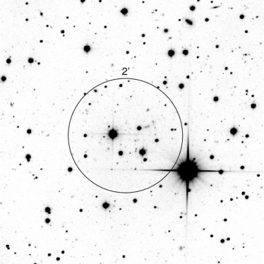
Figure 6: Low-signal instrumental test for the $0.6\,\mathrm{m}$ telescope during the 2015 mission. The image corresponds to a total of $1.5$ hours of luminance exposure. Many galaxies of MACS J0647.7+7015, located at redshift $z=0.584$, are individually resolved, but the elliptic shape of only a few can be guessed.

5 Conclusions

This article presents the results of optical follow-up searches of Planck SZ sources with non-professional $0.5\,\mathrm{m}$ and $0.6\,\mathrm{m}$ telescopes. Our main result is the confirmation of the cluster candidate PSZ2 G156.24+22.32 by observing more than $100$ galaxies within a $3\arcmin$-radius region around the SZ coordinates and by estimating their photometric redshift at $z_{\mathrm{phot}}=0.29\pm 0.08$. We have also estimated the optical richness, $\lambda$, around this location. Although systematics in the photometric zero-points are expected to bias $\lambda$ to lower values, its dependence in redshift allows us to narrow down the cluster’s redshift to $z_{\lambda}=0.30{\,}^{+0.03}_{-0.05}$. Imaging also reveals a contiguous population of galaxies extending a few arcminutes southeast from the SZ region. However, their optical richness suggests that they do not belong to the cluster, and are loosely concentrated around $z\simeq 0.42$.

The robustness of these results have been tested against the choice of the region in which galaxies are counted, the color-redshift relationship, and by removing the $z^{\prime}$ color data. Moreover, photometric redshift estimates of two already confirmed clusters of the PSZ2 catalog, made with the same telescopes, are compatible with their actual redshifts.

The potential of individual sub-meter instruments in the optical confirmation of SZ sources and the measurement of their redshift is obviously limited with respect to what can be achieved with much larger telescopes. However, compared with automated acquisition campaigns, their advantage is the possibility to acquire sensibly deeper data by accumulating longer exposure time over one target (see Sect. 4.1). The present results suggest that observing galaxy overdensity and estimating redshift are achievable in a redshift range $0.1$ to $0.6$, albeit with relatively large uncertainties for the redshift, up to $40\%$ for the closest clusters. In addition, there are potentially hundreds of sub-meter class telescopes available around the world, mostly within the amateur astronomer community. With even a fraction of them, dedicated searches of SZ sources could be collectively envisaged, in a way similar to what the Galaxy Zoo project is providing (Lintott et al., 2008). A case-by-case tuning of the acquisition parameters (unitary exposure time in particular) can be operated to account for the presence of bright objects in the vicinity of the faint galaxies to be detected, which is more complicated to achieve in the case of an automatic survey. Such a collective campaign would certainly bring complementarity to automated surveys. At the very least, such a project could be used to provide a first information on the redshift before starting more accurate investigations with professional telescopes.

References

- Abell (1958) Abell, G. O. 1958, ApJS, 3, 211, doi: 10.1086/190036
- Ahn et al. (2012) Ahn, C. P., Alexandroff, R., Allende Prieto, C., et al. 2012, ApJS, 203, 21, doi: 10.1088/0067-0049/203/2/21
- Arnaud et al. (2007) Arnaud, M., Pointecouteau, E., & Pratt, G. W. 2007, A&A, 474, L37, doi: 10.1051/0004-6361:20078541
- Arnaud et al. (2010) Arnaud, M., Pratt, G. W., Piffaretti, R., et al. 2010, A&A, 517, A92, doi: 10.1051/0004-6361/200913416
- Barr et al. (2005) Barr, J., Davies, R., Jørgensen, I., Bergmann, M., & Crampton, D. 2005, AJ, 130, 445, doi: 10.1086/431745
- Bertin (2006) Bertin, E. 2006, in Astronomical Society of the Pacific Conference Series, Vol. 351, Astronomical Data Analysis Software and Systems XV, ed. C. Gabriel, C. Arviset, D. Ponz, & S. Enrique, 112
- Bertin & Arnouts (1996) Bertin, E., & Arnouts, S. 1996, A&AS, 117, 393, doi: 10.1051/aas:1996164
- Bertin et al. (2002) Bertin, E., Mellier, Y., Radovich, M., et al. 2002, in Astronomical Society of the Pacific Conference Series, Vol. 281, Astronomical Data Analysis Software and Systems XI, ed. D. A. Bohlender, D. Durand, & T. H. Handley, 228
- Bleem et al. (2015) Bleem, L. E., Stalder, B., de Haan, T., et al. 2015, ApJS, 216, 27, doi: 10.1088/0067-0049/216/2/27
- Bunn (2006) Bunn, E. F. 2006, Phys. Rev. D, 73, 123517, doi: 10.1103/PhysRevD.73.123517
- Challinor et al. (2000) Challinor, A. D., Ford, M. T., & Lasenby, A. N. 2000, MNRAS, 312, 159, doi: 10.1046/j.1365-8711.2000.03131.x
- Chambers et al. (2016) Chambers, K. C., Magnier, E. A., Metcalfe, N., et al. 2016, ArXiv e-prints. https://arxiv.org/abs/1612.05560
- Ebeling et al. (2001) Ebeling, H., Edge, A. C., & Henry, J. P. 2001, ApJ, 553, 668, doi: 10.1086/320958
- Fukugita et al. (1996) Fukugita, M., Ichikawa, T., Gunn, J. E., et al. 1996, AJ, 111, 1748, doi: 10.1086/117915
- Gladders & Yee (2000) Gladders, M. D., & Yee, H. K. C. 2000, AJ, 120, 2148, doi: 10.1086/301557
- Graff et al. (2012) Graff, P., Feroz, F., Hobson, M. P., & Lasenby, A. 2012, MNRAS, 421, 169, doi: 10.1111/j.1365-2966.2011.20288.x
- Graff et al. (2014) —. 2014, MNRAS, 441, 1741, doi: 10.1093/mnras/stu642
- Hasselfield et al. (2013) Hasselfield, M., Hilton, M., Marriage, T. A., et al. 2013, J. Cosmology Astropart. Phys, 7, 008, doi: 10.1088/1475-7516/2013/07/008
- Hilton et al. (2017) Hilton, M., Hasselfield, M., Sifón, C., et al. 2017, ArXiv e-prints. https://arxiv.org/abs/1709.05600
- Hobson et al. (2014) Hobson, M., Graff, P., Feroz, F., & Lasenby, A. 2014, in IAU Symposium, Vol. 306, Statistical Challenges in 21st Century Cosmology, ed. A. Heavens, J.-L. Starck, & A. Krone-Martins, 279–287
- Hurier et al. (2017) Hurier, G., Aghanim, N., & Douspis, M. 2017, ArXiv e-prints. https://arxiv.org/abs/1702.00075
- King (1989) King, E. S. 1989, S&T, 77, 387
- Koester et al. (2007) Koester, B. P., McKay, T. A., Annis, J., et al. 2007, ApJ, 660, 221, doi: 10.1086/512092
- Lintott et al. (2008) Lintott, C. J., Schawinski, K., Slosar, A., et al. 2008, MNRAS, 389, 1179, doi: 10.1111/j.1365-2966.2008.13689.x
- Liu et al. (2015) Liu, J., Hennig, C., Desai, S., et al. 2015, MNRAS, 449, 3370, doi: 10.1093/mnras/stv458
- Monet et al. (2003) Monet, D. G., Levine, S. E., Canzian, B., et al. 2003, AJ, 125, 984, doi: 10.1086/345888
- Mullis et al. (2003) Mullis, C. R., McNamara, B. R., Quintana, H., et al. 2003, ApJ, 594, 154, doi: 10.1086/376866
- Piffaretti et al. (2011) Piffaretti, R., Arnaud, M., Pratt, G. W., Pointecouteau, E., & Melin, J.-B. 2011, A&A, 534, A109, doi: 10.1051/0004-6361/201015377
- Planck Collaboration et al. (2014a) Planck Collaboration, Ade, P. A. R., Aghanim, N., et al. 2014a, A&A, 571, A29, doi: 10.1051/0004-6361/201321523
- Planck Collaboration et al. (2014b) —. 2014b, A&A, 571, A20, doi: 10.1051/0004-6361/201321521
- Planck Collaboration et al. (2015a) —. 2015a, A&A, 581, A14, doi: 10.1051/0004-6361/201525787
- Planck Collaboration et al. (2015b) —. 2015b, A&A, 582, A29, doi: 10.1051/0004-6361/201424674
- Planck Collaboration et al. (2016a) —. 2016a, A&A, 594, A27, doi: 10.1051/0004-6361/201525823
- Planck Collaboration et al. (2016b) —. 2016b, A&A, 594, A24, doi: 10.1051/0004-6361/201525833
- Planck Collaboration et al. (2016c) —. 2016c, A&A, 594, A13, doi: 10.1051/0004-6361/201525830
- Planck Collaboration et al. (2016d) —. 2016d, A&A, 586, A139, doi: 10.1051/0004-6361/201526345
- Rozo et al. (2015) Rozo, E., Rykoff, E. S., Bartlett, J. G., & Melin, J.-B. 2015, MNRAS, 450, 592, doi: 10.1093/mnras/stv605
- Rozo et al. (2009) Rozo, E., Rykoff, E. S., Koester, B. P., et al. 2009, ApJ, 703, 601, doi: 10.1088/0004-637X/703/1/601
- Rykoff et al. (2012) Rykoff, E. S., Koester, B. P., Rozo, E., et al. 2012, ApJ, 746, 178, doi: 10.1088/0004-637X/746/2/178
- Rykoff et al. (2014) Rykoff, E. S., Rozo, E., Busha, M. T., et al. 2014, ApJ, 785, 104, doi: 10.1088/0004-637X/785/2/104
- Rykoff et al. (2016) Rykoff, E. S., Rozo, E., Hollowood, D., et al. 2016, ApJS, 224, 1, doi: 10.3847/0067-0049/224/1/1
- Sazonov & Sunyaev (1999) Sazonov, S. Y., & Sunyaev, R. A. 1999, MNRAS, 310, 765, doi: 10.1046/j.1365-8711.1999.02981.x
- Schlafly & Finkbeiner (2011) Schlafly, E. F., & Finkbeiner, D. P. 2011, ApJ, 737, 103, doi: 10.1088/0004-637X/737/2/103
- Schlegel et al. (1998) Schlegel, D. J., Finkbeiner, D. P., & Davis, M. 1998, ApJ, 500, 525, doi: 10.1086/305772
- Smith et al. (2002) Smith, J. A., Tucker, D. L., Kent, S., et al. 2002, AJ, 123, 2121, doi: 10.1086/339311
- Sunyaev & Zeldovich (1980) Sunyaev, R. A., & Zeldovich, I. B. 1980, MNRAS, 190, 413, doi: 10.1093/mnras/190.3.413
- Sunyaev & Zeldovich (1970) Sunyaev, R. A., & Zeldovich, Y. B. 1970, Ap&SS, 7, 3, doi: 10.1007/BF00653471
- Sunyaev & Zeldovich (1972) —. 1972, Comments on Astrophysics and Space Physics, 4, 173
- Tody (1986) Tody, D. 1986, in Proc. SPIE, Vol. 627, Instrumentation in astronomy VI, ed. D. L. Crawford, 733
- Tody (1993) Tody, D. 1993, in Astronomical Society of the Pacific Conference Series, Vol. 52, Astronomical Data Analysis Software and Systems II, ed. R. J. Hanisch, R. J. V. Brissenden, & J. Barnes, 173
- van der Burg et al. (2016) van der Burg, R. F. J., Aussel, H., Pratt, G. W., et al. 2016, A&A, 587, A23, doi: 10.1051/0004-6361/201527299
- Voges et al. (1999) Voges, W., Aschenbach, B., Boller, T., et al. 1999, A&A, 349, 389
- Vorobyev et al. (2016) Vorobyev, V. S., Burenin, R. A., Bikmaev, I. F., et al. 2016, Astronomy Letters, 42, 63, doi: 10.1134/S1063773716020055
- Wen et al. (2012) Wen, Z. L., Han, J. L., & Liu, F. S. 2012, ApJS, 199, 34, doi: 10.1088/0067-0049/199/2/34
- Wenger et al. (2000) Wenger, M., Ochsenbein, F., Egret, D., et al. 2000, A&AS, 143, 9, doi: 10.1051/aas:2000332
- Wright et al. (2010) Wright, E. L., Eisenhardt, P. R. M., Mainzer, A. K., et al. 2010, AJ, 140, 1868, doi: 10.1088/0004-6256/140/6/1868
- York et al. (2000) York, D. G., Adelman, J., Anderson, Jr., J. E., et al. 2000, AJ, 120, 1579, doi: 10.1086/301513
- Zacharias et al. (2015) Zacharias, N., Finch, C., Subasavage, J., et al. 2015, AJ, 150, 101, doi: 10.1088/0004-6256/150/4/101