ROBUST ERROR ESTIMATION FOR LOWEST-ORDER APPROXIMATION OF NEARLY INCOMPRESSIBLE ELASTICITY

Abstract

We consider so-called Herrmann and Hydrostatic mixed formulations of classical linear elasticity and analyse the error associated with locally stabilised $\bm{P}_{1}$–$P_{0}$ finite element approximation. First, we prove a stability estimate for the discrete problem and establish an a priori estimate for the associated energy error. Second, we consider a residual-based a posteriori error estimator as well as a local Poisson problem estimator. We establish bounds for the energy error that are independent of the Lamé coefficients and prove that the estimators are robust in the incompressible limit. A key issue to be addressed is the requirement for pressure stabilisation. Numerical results are presented that validate the theory. The software used is available online.

(xxxxxxxxxx)

AMS Subject Classification: 65N30, 65N15.

1 Introduction

Our starting point is the classical linear boundary value problem modelling the deformation of a homogeneous isotropic elastic body,

$$-\nabla\cdot\mbox{\boldmath$\sigma$} =\bm{f}\quad\mbox{in }\Omega (\mbox{equilibrium of forces}),$$ (1a)

$$\bm{u} ={\bm{g}\quad\mbox{on }\partial\Omega} (\mbox{essential boundary condition}),$$ (1b)

where $\Omega\subset\mathbb{R}^{2}$ is a bounded Lipschitz polygon. Here, the deformation is written in terms of the stress tensor $\mbox{\boldmath$\sigma$}:\hbox{{\msbm\char 82\relax}}^{2}\rightarrow\hbox{{\msbm\char 82\relax}}^{2\times 2}$ and the body force $\bm{f}:\hbox{{\msbm\char 82\relax}}^{2}\rightarrow\hbox{{\msbm\char 82\relax}}^{2}$, where

$$\mbox{\boldmath$\sigma$}=2\mu\bm{\varepsilon}(\bm{u})+\lambda({\nabla\cdot\bm{u}}){\bm{I}},$$

${\bm{I}}$ is the $2\times 2$ identity matrix, $\bm{\varepsilon}:\hbox{{\msbm\char 82\relax}}^{2}\rightarrow\hbox{{\msbm\char 82\relax}}^{2\times 2}$ is the strain tensor, $\bm{u}:\hbox{{\msbm\char 82\relax}}^{2}\rightarrow\hbox{{\msbm\char 82\relax}}^{2}$ is the displacement, and $\bm{\varepsilon}(\bm{u})=\frac{1}{2}(\nabla\bm{u}+(\nabla\bm{u})^{\top})$. The Lamé coefficients $\mu$ and $\lambda$ satisfy $0<\mu_{1}<\mu<\mu_{2}<\infty$ and $0<\lambda<\infty$ and can be written in terms of the Young’s modulus $E$ and the Poisson ratio $\nu$ as

$$\mu=\frac{E}{2(1+\nu)},\quad\lambda=\frac{E\nu}{(1+\nu)(1-2\nu)}.$$

The coefficient $\lambda$ becomes unbounded in the incompressible limit $\nu\to 1/2$, leading to the well-known phenomenon of locking for standard finite element methods. A popular remedy is to introduce an additional unknown, rewrite (1a)–(1b) as a system and then apply an appropriate mixed finite element method.

We consider mixed approximation methods that are robust with respect to the Lamé coefficients which arise from the Herrmann or Hydrostatic formulations [4, 11] of (1a)–(1b). Introducing $p=-\kappa\nabla\cdot\mathbf{u}$ we rewrite the problem as

$$-\nabla\cdot\mbox{\boldmath$\sigma$} =\bm{f}\quad\mbox{in }\Omega,$$ (2a)

$$\nabla\cdot\bm{u}+\frac{p}{\kappa} =0\quad\mbox{in }\Omega,$$ (2b)

$$\bm{u} ={\bm{g}\quad\mbox{on }\partial\Omega},$$ (2c)

where either $\kappa=\lambda$ (in the Herrmann formulation) or $\kappa=\mu+\lambda$ (in the Hydrostatic formulation in two dimensions). The stress tensor can then be written as

$$\mbox{\boldmath$\sigma$}(\bm{u},p)=\left\{\begin{array}[]{ll}2\mu\bm{\varepsilon}(\bm{u})-p{\bm{I}}&\quad\mbox{ (Herrmann)},\\ 2\mu(\bm{\varepsilon}(\bm{u})-\frac{1}{2}(\nabla\cdot\bm{u})\bm{I})-p{\bm{I}}&\quad\,\mbox{(Hydrostatic)}.\end{array}\right.$$ (5)

There is an extensive literature on finite element approximation of elasticity problems; see Boffi et al.[3] and Hughes[13] for a comprehensive overview and Houston et al.[12] and Kouhia & Stenberg[17] for specific details. In Ref. KPS, the authors provide a posteriori error analysis for conforming mixed finite element approximations of the Herrmann formulation using stable rectangular elements. A variety of local problem error estimators for the energy error are considered and proved to be robust when $\nu\to 1/2$. Those results can be extended to the Hydrostatic formulation whenever the chosen finite element spaces satisfy minimal conditions, as discussed by Boffi & Stenberg[4]. In this work, we extend the analysis in Ref. KPS to cover the lowest-order $\bm{P}_{1}$–$P_{0}$ approximation defined on triangular elements. An important issue that will be addressed is the requirement for pressure stabilisation. While pressure stabilisation of the lowest order mixed methods for the Stokes equations has been extensively studied (for example by Dohrmann & Bochev[8], Burman & Fernández[5] and Barrenechea & Valentin[2]) the application of stabilised methods to elasticity equations appears to be a new development.

In Section 2 we review the weak formulation of (2). In Section 3, we discuss $\bm{P}_{1}$–$P_{0}$ approximation, review our local stabilisation strategy and establish an a priori error bound. The stabilisation strategy that is adopted was developed in Refs. DD,ks92 in the context of the Stokes equations. The distinctive feature of this contribution is the identification of a suitable energy norm—which removes the requirement to specify (or “tune”) a stabilisation parameter. In Section 4 we discuss a conventional residual-based a posteriori error estimator and we introduce a local Poisson problem estimator. Both estimators are shown to be robust in the sense that the material parameters do not appear in the error bounds. This robustness is significantly more challenging to achieve than for the Stokes problem, which only involves a single (viscosity) parameter. Some numerical results that reinforce the theory are discussed in Section 5. In the rest of the paper we will use the symbols $\lesssim$ and $\gtrsim$ to denote bounds that are valid up to positive constants that are independent of the Lamé coefficients and the mesh parameters.

2 Weak Formulation

Our notation is standard: $H^{s}(\omega)$ denotes the usual Sobolev space with norm $||\cdot||_{s,\omega}$ for $s\geq 0$. When $\omega=\Omega$, we use $||\cdot||_{s}$ instead of $||\cdot||_{s,\Omega}$ and we denote vector-valued Sobolev spaces by boldface letters $\bm{H}^{s}(\omega)=\bm{H}^{s}(\omega;\hbox{{\msbm\char 82\relax}}^{2})$. We also define

$$\bm{H}^{1}_{E}(\Omega):=\bigl{\{}\bm{v}\in\bm{H}^{1}(\Omega)\;\big{|}\;\bm{v}|_{\partial\Omega}=\bm{g}\bigr{\}},\quad\bm{H}^{1\over 2}(\partial\Omega):=\bigl{\{}\bm{v}\,|\,\bm{v}=\bm{u}|_{\partial\Omega},\bm{u}\in\bm{H}^{1}(\Omega)\bigr{\}},$$

and the test spaces ${\bm{V}=\bm{H}_{0}^{1}(\Omega):=\bigl{\{}\bm{v}\in\bm{H}^{1}(\Omega)\;\big{|}\;\bm{v}|_{\partial\Omega}=\bm{0}\bigr{\}}}$ and $Q={{\color[rgb]{0,0,0}L^{2}(\Omega)}}$.

The standard weak formulation of (2) is: find $(\bm{u},p)\in\bm{H}^{1}_{E}\times Q$ such that

$$a(\bm{u},\bm{v})+b(\bm{v},p) =f(\bm{v})\quad\forall\bm{v}\in\bm{V},$$ (6a)

$$b(\bm{u},q)-c(p,q) =0\quad\quad\,\forall q\in Q,$$ (6b)

where

$$b(\bm{v},p)=-\int_{\Omega}p\nabla\cdot\bm{v},\quad c(p,q)=\frac{1}{\kappa}\int_{\Omega}pq,\quad f(\bm{v})=\int_{\Omega}\bm{f}\,\bm{v},$$

and either

$$a(\bm{u},\bm{v})=a_{H}(\bm{u},\bm{v})=2\mu\int_{\Omega}\bm{\varepsilon}(\bm{u}):\bm{\varepsilon}(\bm{v}),$$

(in the Herrmann formulation) or

$$a(\bm{u},\bm{v})=a_{S}(\bm{u},\bm{v})=2\mu\left(\int_{\Omega}\bm{\varepsilon}(\bm{u}):\bm{\varepsilon}(\bm{v})-\frac{1}{2}\int_{\Omega}(\nabla\cdot\bm{u})(\nabla\cdot\bm{v})\right)$$

(in the Hydrostatic formulation). Note that, where it is necessary to make a distinction, we will use the notation $a_{H}(\cdot,\cdot)$ and $a_{S}(\cdot,\cdot)$, but where a stated result holds for both, we will simply use $a(\cdot,\cdot)$. We assume $\bm{f}\in(L^{2}(\Omega))^{2}$ and that $\bm{g}\in\bm{H}^{1\over 2}(\partial\Omega)$ is a polynomial of degree at most one in each component so that no error is incurred in approximating the essential boundary condition. As usual, we define

$$\mathcal{B}(\bm{u},p;\bm{v},q)=a(\bm{u},\bm{v})+b(\bm{v},p)+b(\bm{u},q)-c(p,q),$$ (7)

so as to express (6) in the more compact form: find $(\bm{u},p)\in\bm{H}^{1}_{E}\times Q$ such that

$$\mathcal{B}(\bm{u},p;\bm{v},q)=f(\bm{v}),\quad\forall(\bm{v},q)\in\bm{V}\times Q.$$ (8)

Finally, we define the following energy norm for the error analysis

$$|||(\bm{u},p)|||^{2} =2\mu\,{||\nabla\bm{u}||^{2}_{0}}+(2\mu)^{-1}||p||^{2}_{0}+\kappa^{-1}||p||^{2}_{0}.$$ (9)

One can establish the well-posedness of the weak formulation for $\nu\in(0,1/2)$ by considering (6) or (8). We will work with the latter. Note that when $\nu=1/2$, $c(\cdot,\cdot)$ disappears from (6) and the problem can be analysed as a saddle point problem in the standard way (similar to Stokes problems). However, since we impose $\bm{u}=\bm{g}$ on the whole boundary, the pressure solution is only unique up to a constant in that case. We start by reviewing some useful results. For both formulations, it is is easy to show that

$$a(\bm{u},\bm{v})\leq{2\mu}\,{||\nabla\bm{u}||_{0}}\,\,{||\nabla\bm{v}||_{0}}\quad\forall\bm{u},\bm{v}\in\bm{V}.$$ (10)

It is also known that that there exists an (inf-sup) constant $C_{\Omega}>0$ such that

$$\sup_{0\neq\bm{v}\in\bm{V}}\frac{b(\bm{v},q)}{||\nabla\bm{v}||_{0}}\geq C_{\Omega}||q||_{0},\quad{\forall q\in{Q},q\neq{\rm constant},}$$ (11)

see, for example, p. 128 of Ref. HDA. Next, in the Herrmann formulation, we know that

$$a_{H}(\bm{v},\bm{v}) \geq C_{K}2\mu\,{||\nabla\bm{v}||_{0}^{2}}\quad\forall\bm{v}\in\bm{V},$$ (12)

by Korn’s inequality, so that $a_{H}(\cdot,\cdot)$ is coercive on $\bm{V}$. Similarly, in the Hydrostatic case[4] we have that

$$a_{S}(\bm{v},\bm{v}) \geq(1/2)2\mu\,{||\nabla\bm{v}||_{0}^{2}}\quad\forall\bm{v}\in\bm{V}.$$ (13)

We note in passing that the coercivity estimate (13) does not hold if $\partial\Omega=\partial\Omega_{D}\cup\partial\Omega_{N}$, where $\partial\Omega_{N}\neq\emptyset$ is a portion of the boundary where $\bm{\sigma}\bm{n}=\bm{0}$. (This case requires a separate treatment, exploiting the fact that $a_{S}(\cdot,\cdot)$ is coercive on an appropriate nullspace $\bm{V}_{0}\subset\bm{V}$.)

The following stability result ensures well-posedness of (8).

Lemma 2.1.

Let ${{\color[rgb]{0,0,0}Q_{0}}}:=\left\{q\in{{\color[rgb]{0,0,0}L^{2}(\Omega)}},\int_{\Omega}q=0\right\}$. For any $(\bm{u},p)\in\bm{V}\times{{\color[rgb]{0,0,0}Q_{0}}}$, there exists a pair of functions $(\bm{v},q)\in\bm{V}\times{{\color[rgb]{0,0,0}Q_{0}}}$, with $|||(\bm{v},q)|||\lesssim|||(\bm{u},p)|||$, satisfying

$$\mathcal{B}(\bm{u},p;\bm{v},q)\gtrsim|||(\bm{u},p)|||^{{2}}.$$

Proof 2.2.

For the Herrmann case, the result follows from (10), (11) and (12); see Lemma 3.3 in Ref. KPS. In the Hydrostatic case, the same proof can be applied, using (13) instead of (12) (which is the same result with $C_{K}=1/2$). Since the energy norm (9) is defined with respect to $\kappa$, the constant in the bound $\gtrsim$ is the same (up to the value of $C_{K}$).

Remark 2.3.

To check the uniqueness of the pressure solution for $\nu\in(0,1/2)$ we test (6b) with a constant function ${{\color[rgb]{0,0,0}q=1}}$ and use the divergence theorem. This gives

$$\frac{1}{\kappa}\int_{\Omega}p\> =-\int_{\Omega}\nabla\cdot\bm{u}={{\color[rgb]{0,0,0}-}}\int_{\partial\Omega}\bm{u}\cdot\bm{n}\,ds,\quad\hbox{thus}\quad\int_{\Omega}p\>=-\kappa\int_{\partial\Omega}\bm{g}\cdot\bm{n}\,ds.$$ (14)

The characterisation (14) guarantees the uniqueness of the pressure satisfying (8) using either of the two formulations.

3 Stabilised $P_{1}$–$P_{0}$ approximation

Let $\{\mathcal{T}_{h}\}$ denote a family of shape-regular triangular meshes of ${{\color[rgb]{0,0,0}\overline{\Omega}}}$ into triangles $K$ of diameter $h_{K}$. For each mesh $\mathcal{T}_{h}$, we let $\mathcal{E}_{h}$ denote the set of all edges and $h_{E}$ denote the length of an edge $E\in\mathcal{E}_{h}$. Next, we introduce finite-dimensional subsets $\bm{X}^{h}_{E}\subset\bm{H}^{1}_{E}$, $\bm{X}^{h}_{0}\subset\bm{V}$ and $Q^{h}\subset Q$. The discrete weak formulation of (6) is as follows: find $(\bm{u}_{h},p_{h})\in\bm{X}^{h}_{E}\times Q^{h}$ such that

$$a(\bm{u}_{h},\bm{v}_{h})+b(\bm{v}_{h},p_{h}) =f(\bm{v}_{h})\quad\forall\bm{v}_{h}\in\bm{X}^{h}_{0},$$ (15a)

$$b(\bm{u}_{h},q_{h})-c(p_{h},q_{h}) =0\quad\quad\;\;\forall q_{h}\in Q^{h}.$$ (15b)

Specifically, we choose $\bm{X}^{h}_{0}$ to be the space of vector-valued functions that are piecewise linear in each component and globally continuous ($\bm{P}_{1}$), and we choose $Q^{h}$ to be the subset of $Q$ that contains piecewise constant functions ($P_{0}$). The solution space $\bm{X}^{h}_{E}$ is obtained from $\bm{X}^{h}_{0}$ by construction in the usual way, by augmenting the basis with additional $\bm{P}_{1}$ functions associated with Dirichlet boundary nodes (where $\bm{g}\neq\bm{0}$). For more details about $\bm{P}_{1}$–${P}_{0}$ approximation, see Refs. HDA,DD,DFM,ks92,ns98. We note that, while the simplicity of the low-order scheme is very attractive from a computational point of view, stabilisation of the underlying approximation is essential when working with values of $\nu$ close to $1/2$.

Given a mesh $\mathcal{T}_{h}$, to define our stabilisation strategy, we first select a macroelement partitioning $\mathcal{M}_{h}$ which satisfies:

1. Each macroelement $M\in\mathcal{M}_{h}$ is a connected set of adjoining elements from $\mathcal{T}_{h}$.

2. $M_{i}\cap M_{j}=\emptyset$ for all $M_{i},M_{j}\in\mathcal{M}_{h},\,i\neq j$.

3. For any two neighboring macroelements $M_{1}$ and $M_{2}$ with $\int_{M_{1}\cap M_{2}}ds\neq 0$, there exists $\bm{v}\in{{\color[rgb]{0,0,0}\bm{X}^{h}_{0}}}$ such that supp $\bm{v}\subset\overline{M}_{1}\cup\overline{M}_{2}$ and $\int_{M_{1}\cap M_{2}}\bm{v}\cdot\bm{n}\,ds\neq 0$.

4. $\cup_{M\in\mathcal{M}_{h}}\overline{M}={{\color[rgb]{0,0,0}\overline{\Omega}}}$. For each $M\in\mathcal{M}_{h}$, the set of interior interelement edges will be denoted by $\Gamma_{M}$. That is,

   $$\Gamma_{M}=\{E\in\mathcal{E}_{h}\setminus\partial\Omega,E\subset M\}.$$

With the above definition, a locally stabilised version of the discrete weak problem (15) is as follows: find $(\bm{u}_{h},p_{h})\in\bm{X}^{h}_{E}\times Q^{h}$ such that

$$a(\bm{u}_{h},\bm{v}_{h})+b(\bm{v}_{h},p_{h}) =f(\bm{v}_{h})\quad\forall\bm{v}_{h}\in\bm{X}^{h}_{0},$$ (16a)

$$b(\bm{u}_{h},q_{h})-c(p_{h},q_{h})-\mathcal{C}_{loc}(p_{h},q_{h}) =0,\quad\quad\;\;\forall q_{h}\in Q^{h},$$ (16b)

where

$$\mathcal{C}_{loc}(p_{h},q_{h})=\frac{1}{2\mu}\sum_{M\in\mathcal{M}_{h}}\sum_{E\in\Gamma_{M}}h_{E}\int_{E}\llbracket p_{h}\rrbracket\llbracket q_{h}\rrbracket ds,\qquad p_{h},q_{h}\in Q^{h},$$

and $\llbracket\cdot\rrbracket$ denotes the jump across $E\in\Gamma_{M}$.

Remark 3.1.

The choice of the stabilisation parameter $(1/2\mu)$ in the definition of $\mathcal{C}_{loc}(\cdot,\cdot)$ is motivated by the a priori error analysis presented next.

The discrete pressure $p_{h}\in Q^{h}$ that solves (16) is not uniquely defined in the limiting case $\nu=1/2$. The associated linear algebra system is singular in this case. Define the constrained pressure approximation space $Q_{0}^{h}=Q^{h}\cap Q_{0}$. We will assume that for any partitioning ${\mathcal{M}}_{h}$, each macroelement $M\in{\mathcal{M}}_{h}$ belongs to one of a finite number of possible equivalence classes $\mathcal{E}_{\hat{M}_{1}},\ldots,\mathcal{E}_{\hat{M}_{N}}$. The next result immediately follows from Lemma 3.1 in Ref. ks92.

Lemma 3.2.

Let $\Pi_{h}$ be the $L^{2}$ projection operator from ${{\color[rgb]{0,0,0}Q_{0}^{h}}}$ onto the subspace

$${{\color[rgb]{0,0,0}\overline{Q}}}^{\,h}=\{q\in{{\color[rgb]{0,0,0}Q_{0}}},\,q|_{M}\,\mbox{ is {{\color[rgb]{0,0,0}constant}} }\forall M\in\mathcal{M}_{h}\}.$$ (17)

Then, there exists $\alpha_{1}>0$ independent of $h$ and the Lamé coefficients satisfying

$$\mathcal{C}_{loc}(q,q)\geq\alpha_{1}\frac{1}{2\mu}||(I-\Pi_{h})q||_{0}^{2}\quad\forall q\in{{\color[rgb]{0,0,0}Q_{0}^{h}}}.$$

The stabilised discrete formulation (16) can also be written as: find $(\bm{u}_{h},p_{h})\in\bm{X}^{h}_{E}\times Q^{h}$ such that

$$\mathcal{B}_{S}(\bm{u}_{h},p_{h};\bm{v}_{h},q_{h})=f(\bm{v}_{h}),\quad\forall(\bm{v}_{h},q_{h})\in\bm{X}^{h}_{0}\times Q^{h},$$ (18)

which involves the stabilised bilinear form

$$\mathcal{B}_{S}(\bm{u}_{h},p_{h};\bm{v}_{h},q_{h})=a(\bm{u}_{h},\bm{v}_{h})+b(\bm{v}_{h},p_{h})+b(\bm{u}_{h},q_{h})-c(p_{h},q_{h})-\mathcal{C}_{loc}(p_{h},q_{h}).$$

We are now ready to prove a stability result for (18).

Lemma 3.3.

For any $(\bm{u},p)\in\bm{X}^{h}_{0}\times{{\color[rgb]{0,0,0}Q_{0}^{h}}}$, there exists a pair of functions $(\bm{v},q)\in\bm{X}^{h}_{0}\times{{\color[rgb]{0,0,0}Q_{0}^{h}}}$ with $|||(\bm{v},q)|||\lesssim|||(\bm{u},p)|||$ satisfying

$$\mathcal{B}_{S}(\bm{u},p;\bm{v},q)\gtrsim|||(\bm{u},p)|||^{2}.$$

Proof 3.4.

A consequence of (11) is that there exists a constant $\alpha_{2}$, independent of $h$ and the Lamé coefficients, and a function $\bm{w}\in\bm{X}^{h}_{0}$ satisfying

$$(\Pi_{h}p,\nabla\cdot\bm{w})=(2\mu)^{-1}||\Pi_{h}p||_{0}^{2},\quad(2\mu)^{1/2}||\nabla\bm{w}||_{0}\leq\alpha_{2}(2\mu)^{-1/2}||\Pi_{h}p||_{0}.$$ (19)

Since $(\bm{u},p)\in\bm{X}^{h}_{0}\times{{\color[rgb]{0,0,0}Q_{0}^{h}}}$ and $\bm{X}_{0}^{h}\subset\bm{V}$, ${{\color[rgb]{0,0,0}Q_{0}^{h}\subset Q^{h}}}$, using the definition of $\mathcal{B}_{S}(\cdot,\cdot)$ gives,

$$\mathcal{B}_{S}(\bm{u},p;\bm{u},-p) \geq C_{K}2\mu||\nabla\bm{u}||^{2}_{0}+\kappa^{-1}||p||^{2}_{0}+\mathcal{C}_{loc}(p,p),$$ (20)

by (12) (Herrmann case) or (13) (Hydrostatic case). Next, using (19) and (10), for any $\epsilon>0$ we have,

$$\mathcal{B}_{S}(\bm{u},p;-\bm{w},0) =-a(\bm{u},\bm{w})-b(\bm{w},(I-\Pi_{h})p)-b(\bm{w},\Pi_{h}p)$$

$$\geq-(2\mu)^{\frac{1}{2}}||\nabla\bm{u}||_{0}\;(2\mu)^{\frac{1}{2}}||\nabla\bm{w}||_{0}$$

$$\quad-(2\mu)^{-\frac{1}{2}}||(I-\Pi_{h})p||_{0}(2\mu)^{\frac{1}{2}}||\nabla\bm{w}||_{0}\ +(2\mu)^{-1}||\Pi_{h}p||^{2}_{0}$$

$$\geq-(2\mu)^{1/2}||\nabla\bm{u}||_{0}\;\alpha_{2}(2\mu)^{-1/2}||\Pi_{h}p||_{0}$$

$$\quad-(2\mu)^{-1/2}||(I-\Pi_{h})p||_{0}(2\mu)^{-1/2}\alpha_{2}||\Pi_{h}p||_{0}+(2\mu)^{-1}||\Pi_{h}p||^{2}_{0},$$

$$\geq-\epsilon(2\mu)||\nabla\bm{u}||^{2}_{0}-2\epsilon^{-1}\alpha_{2}^{2}(2\mu)^{-1}||\Pi_{h}p||_{0}^{2}$$

$$\quad-\epsilon(2\mu)^{-1}||(I-\Pi_{h})p||_{0}^{2}+(2\mu)^{-1}||\Pi_{h}p||^{2}_{0}.$$ (21)

Now we introduce a parameter $\delta$. Using Lemma 3.2, (20) and (3.4) we have,

$$\mathcal{B}_{S}(\bm{u},p;\bm{u}-\delta\bm{w},-p) =\mathcal{B}(\bm{u},p;\bm{u},-p)+\delta\mathcal{B}(\bm{u},p;-\bm{w},0)$$

$$\geq C_{K}2\mu||\nabla\bm{u}||^{2}_{0}+\kappa^{-1}||p||^{2}_{0}+\mathcal{C}_{loc}(p,p)+\delta(2\mu)^{-1}||\Pi_{h}p||^{2}_{0}$$

$$-2\mu\delta\epsilon||\nabla\bm{u}||^{2}_{0}-2\delta\epsilon^{-1}\alpha_{2}^{2}(2\mu)^{-1}||\Pi_{h}p||_{0}^{2}-\delta\epsilon(2\mu)^{-1}||(I-\Pi_{h})p||_{0}^{2},$$

$$\geq(C_{K}-\delta\epsilon)2\mu||\nabla\bm{u}||^{2}_{0}+\kappa^{-1}||p||^{2}_{0}+\delta\left(1-2\alpha_{2}^{2}\epsilon^{-1}\right)(2\mu)^{-1}||\Pi_{h}p||^{2}_{0}$$

$$\quad-\delta\epsilon(2\mu)^{-1}||(I-\Pi_{h})p||_{0}^{2}+\alpha_{1}(2\mu)^{-1}||(I-\Pi_{h})p||_{0}^{2},$$

$$\geq(C_{K}-\delta\epsilon)2\mu||\nabla\bm{u}||^{2}_{0}+\kappa^{-1}||p||^{2}_{0}+\delta\left(1-\ 2\alpha_{2}^{2}\epsilon^{-1}\right)(2\mu)^{-1}||\Pi_{h}p||^{2}_{0}$$

$$\quad+(\alpha_{1}-\delta\epsilon)(2\mu)^{-1}||(I-\Pi_{h})p||_{0}^{2}.$$

Making the specific choices $\epsilon=4\alpha_{2}^{2}$ and $\delta=\frac{1}{4\alpha_{2}^{2}}\min\{C_{K}/2,\alpha_{1}/2\}$, it follows:

$$\mathcal{B}_{S}(\bm{u},p;\bm{u}-\delta\bm{w},-p) \geq C\left(2\mu||\nabla\bm{u}||^{2}_{0}+\frac{1}{\kappa}||p||^{2}_{0}+(2\mu)^{-1}\left(||\Pi_{h}p||^{2}_{0}+||(I-\Pi_{h})p||_{0}^{2}\right)\right),$$

$$\geq C\left(2\mu||\nabla\bm{u}||^{2}_{0}+\frac{1}{\kappa}||p||^{2}_{0}+(2\mu)^{-1}||p||^{2}_{0}\right),$$ (22)

where $C=\min\left\{1,\frac{C_{K}}{2},\frac{\alpha_{1}}{2},\frac{\delta}{2}\right\}$. Hence, the result holds with $\bm{v}=\bm{u}-\delta\bm{w}$ and $q=-p$. Finally, using the definition of $|||\cdot|||$ and (19) gives

$$|||(\bm{v},q)|||^{2} =2\mu\|\nabla\left(\bm{u}-\delta\bm{w}\right)\|_{0}^{2}+(2\mu)^{-1}\|p\|_{0}^{2}+\kappa^{-1}\|p\|_{0}^{2}$$

$$\leq 2(2\mu)||\nabla\bm{u}||_{0}^{2}+2(2\mu)\delta^{2}||\nabla\bm{w}||_{0}^{2}+\left(\kappa^{-1}+(2\mu)^{-1}\right)||p||^{2}_{0},$$

$$\leq\left(2+\frac{\delta^{2}\alpha_{2}^{2}}{2}\right)|||(\bm{u},p)|||^{2}.$$ (23)

The constants in (3.4) and (3.4) are independent of the Lamé coefficients.

We can now establish an a priori bound for the energy norm of the error associated with the stabilised $\bm{P}_{1}$–$P_{0}$ approximation.

Theorem 3.5.

Let ${{\color[rgb]{0,0,0}(\bm{u},p)\in\bm{H}^{1}_{E}\times Q}}$ be the solution to (6) and let $(\bm{u}_{h},p_{h})\in\bm{X}^{h}_{E}\times Q^{h}$ satisfy (16). Suppose that $\int_{\partial\Omega}\bm{g}\cdot\bm{n}\,ds=0$ so that $\int_{\Omega}p=0=\int_{\Omega}p_{h}$ from (14). If $\bm{u}\in\bm{H}^{2}(\Omega)$ and $p\in H^{1}(\Omega)$, then

$$|||(\bm{u}-\bm{u}_{h},p-p_{h})|||\lesssim h\left((2\mu)^{1/2}|\bm{u}|_{2}+\left((2\mu)^{-1/2}+\kappa^{-1/2}\right)|p|_{1}\right).$$ (24)

Proof 3.6.

Let $\tilde{\bm{u}}\in\bm{X}^{h}_{E}$ represent the piecewise linear interpolant of $\bm{u}\in\bm{H}^{1}_{E}$ and let $\tilde{p}\in Q^{h}_{0}$ be the piecewise constant projection of $p\in Q$ with mean value zero. Using the triangle inequality gives

$$|||(\bm{u}-\bm{u}_{h},p-p_{h})|||\,\lesssim\,|||(\bm{u}-\tilde{\bm{u}},p-\tilde{p})|||+|||(\tilde{\bm{u}}-\bm{u}_{h},\tilde{p}-p_{h})|||,$$ (25)

and the interpolation error satisfies

$$|||(\bm{u}-\tilde{\bm{u}},p-\tilde{p})|||\,\lesssim\,h\left((2\mu)^{1/2}|\bm{u}|_{2}+\left((2\mu)^{-1/2}+\kappa^{-1/2}\right)|p|_{1}\right).$$ (26)

Now, for all $(\bm{v},q)\in\bm{X}^{h}_{0}\times Q^{h}$, using (8) and (18), gives

$$\mathcal{B}_{S}(\bm{u}_{h}-\tilde{\bm{u}},p_{h}-\tilde{p};\bm{v},q) =\mathcal{B}_{S}(\bm{u}_{h},p_{h};\bm{v},q)-\mathcal{B}(\tilde{\bm{u}},\tilde{p};\bm{v},q)+\mathcal{C}_{loc}(\tilde{p},q)$$

$$=\mathcal{B}(\bm{u},p;\bm{v},q)-\mathcal{B}(\tilde{\bm{u}},\tilde{p};\bm{v},q)+\mathcal{C}_{loc}(\tilde{p},q)$$

$$=\mathcal{B}(\bm{u}-\tilde{\bm{u}},p-\tilde{p};\bm{v},q)+\mathcal{C}_{loc}(\tilde{p},q).$$

Since $(\bm{u}_{h}-\tilde{\bm{u}},p_{h}-\tilde{p})\in{{\color[rgb]{0,0,0}\bm{X}_{0}^{h}\times{{\color[rgb]{0,0,0}Q_{0}^{h}}}}}$, applying Lemma 3.3 in the usual way gives

$$|||(\bm{u}_{h}-\tilde{\bm{u}},p_{h}-\tilde{p})|||\lesssim|||\left(\bm{u}-\tilde{\bm{u}},p-\tilde{p}\right)|||+\sup_{{{\color[rgb]{0,0,0}q\in Q_{0}^{h}}},(2\mu)^{-1/2}||q||_{0}=1}\mathcal{C}_{loc}(\tilde{p},q).$$

If $p\in H^{1}(\Omega)$, then $\mathcal{C}_{loc}({p},q)=0$ and the Cauchy–Schwarz inequality gives

$$\mathcal{C}_{loc}(\tilde{p},q)=\mathcal{C}_{loc}(\tilde{p}-p,q)\lesssim\Bigg{(}\sum_{K\in\mathcal{T}_{h}}\frac{h_{K}}{{2\mu}}||p-\tilde{p}||_{0,\partial K}^{2}\Bigg{)}^{1/2}\Bigg{(}\sum_{K\in\mathcal{T}_{h}}\frac{h_{K}}{{2\mu}}||q||_{0,\partial K}^{2}\Bigg{)}^{1/2}.$$

Following the proof of Theorem 3.1 in Ref. ks92, it follows that

$$\left(\sum_{K\in\mathcal{T}_{h}}\frac{h_{K}}{2\mu}||q||_{0,\partial K}^{2}\right)^{1/2}\lesssim\frac{1}{\sqrt{2\mu}}||q||_{0},\quad\Bigg{(}\sum_{K\in\mathcal{T}_{h}}\frac{h_{K}}{{2\mu}}||p-\tilde{p}||_{0,\partial K}^{2}\Bigg{)}^{1/2}\lesssim\frac{h}{\sqrt{2\mu}}|p|_{1},$$

and hence

$$|||(\bm{u}_{h}-\tilde{\bm{u}},p_{h}-\tilde{p})|||\lesssim|||\left(\bm{u}-\tilde{\bm{u}},p-\tilde{p}\right)|||+\frac{h}{\sqrt{2\mu}}|p|_{1}.$$ (27)

Combining (25) with (26) and (27) gives the final result.

4 A posteriori error analysis

Two alternative a posteriori energy error estimation strategies will be discussed here. Both estimation strategies are robust in the sense that material parameters do not appear in the error bounds. The proofs are presented here for completeness—they are a minor extension of the results established in Ref. KPS.

4.1 Residual error estimation

We discuss a residual-based error estimator first. The definition involves three distinct parameters:

$$\rho_{K}=h_{K}(2\mu)^{-\frac{1}{2}},\quad\rho_{E}=h_{E}(2\mu)^{-1},\quad\rho_{d}={1/(\kappa^{-1}+(2\mu)^{-1})}.$$ (28)

Let $(\bm{u}_{h},p_{h})\in\bm{X}^{h}_{E}\times Q^{h}$ satisfy (16) and let $\bm{f}_{h}$ be the $L^{2}$-projection of $\bm{f}$ onto the space of piecewise constant functions. For each element $K$ in the finite element mesh $\mathcal{T}_{h}$, we define the local data oscillation error $\bm{\Theta}_{K}$ satisfying

$$\bm{\Theta}_{K}^{2}=\rho_{K}^{2}||\bm{f}-\bm{f}_{h}||^{2}_{0,K},$$ (29)

and a local error indicator $\eta_{K}$ satisfying $\eta^{2}_{K}=\eta^{2}_{R_{K}}+\eta^{2}_{E_{K}}+\eta_{J_{K}}^{2}$, where

$$\eta^{2}_{R_{K}}=\rho_{K}^{2}||\bm{R}_{K}||^{2}_{0,K},\quad\eta^{2}_{J_{K}}=\rho_{d}||R_{K}||^{2}_{0,K}\quad\mbox{and}\quad\eta^{2}_{E_{K}}=\sum_{E\in{{\color[rgb]{0,0,0}\partial K}}}\rho_{E}||\bm{R}_{E}||^{2}_{0,E}.$$ (30)

The two element residuals associated with (2) are given by

$$\bm{R}_{K}=\bm{f}_{h}\big{|}_{K},\quad R_{K}={{\color[rgb]{0,0,0}\left\{\nabla\cdot\bm{u}_{h}+\frac{p_{h}}{\kappa}\right\}\Big{|}_{K}}},$$ (31)

and the edge residual $\bm{R}_{E}$ is associated with the normal stress jump. That is,

$$\bm{R}_{E}=\left\{\begin{array}[]{ll}\frac{1}{2}\llbracket-\bm{\sigma}(\bm{u}_{h},p_{h})\bm{n}\rrbracket_{E}&\quad E\in\mathcal{E}_{h}\setminus\partial\Omega,\\ 0&\quad{E\in\partial\Omega},\end{array}\right.$$ (34)

where $\bm{\sigma}(\bm{u}_{h},p_{h})$ is defined via (5). Note that since $\bm{u}_{h}\in\bm{P}_{1}$ and $p_{h}\in P_{0}$, $\nabla\cdot\bm{u}_{h}$ and $R_{K}$ are constant on each element, as is the normal stress jump on each edge (in both formulations). Hence, $\eta_{K}$ is straightforward to compute. Finally, we sum the element contributions to give the residual error estimator and data oscillation error respectively,

$$\eta=\left(\sum_{K\in\mathcal{T}_{h}}\eta_{K}^{2}\right)^{1/2}\quad\hbox{and}\quad\bm{\Theta}=\left(\sum_{K\in\mathcal{T}_{h}}\bm{\Theta}_{K}^{2}\right)^{1/2}.$$ (35)

Remark 4.1.

The nonuniqueness of the pressure solution in the incompressible limit is not seen by the error estimator ($p_{h}$ drops out of $R_{k}$ when $\lambda\to\infty$ and $\bm{R}_{E}$ measures inter-element jumps in the pressure).

Theorems 4.3 and 4.5 show that $\eta$ is a reliable and efficient estimator for the energy error associated with locally stabilised $\bm{P}_{1}$–$P_{0}$ approximations of (6). The following standard result is needed for Theorem 4.3.

Lemma 4.2 (Clément interpolation).

Given $\bm{v}\in\bm{V},$ let $\bm{v}_{h}\in\bm{X}^{h}_{0}$ be the quasi-interpolant of $\bm{v}$ defined by averaging[7]. For any $K\in\mathcal{T}_{h}$,

$$\rho^{-1}_{K}||\bm{v}-\bm{v}_{h}||_{0,K} \lesssim(2\mu)^{1/2}|\bm{v}|_{1,\omega_{K}},$$

where $|\cdot|_{1,\omega_{K}}$ is the $H^{1}(\omega_{K})$ seminorm. Moreover, for all $E\in\partial K$ we have

$$\rho^{-1/2}_{E}||\bm{v}-\bm{v}_{h}||_{0,E} \lesssim(2\mu)^{1/2}|\bm{v}|_{1,\omega_{K}},$$

where $\omega_{K}$ is the set of triangles sharing at least one vertex with $K$.

Theorem 4.3.

Suppose that ${{\color[rgb]{0,0,0}(\bm{u},p)\in\bm{H}^{1}_{E}\times Q}}$ is the weak solution satisfying (6) and $(\bm{u}_{h},p_{h})\in\bm{X}^{h}_{E}\times Q^{h}$ satisfies (16). Suppose further that $\int_{\partial\Omega}\bm{g}\cdot\bm{n}\,ds=0$ so that $\int_{\Omega}p=0=\int_{\Omega}p_{h}$ from (14). Defining $\eta$ and $\bm{\Theta}$ as in (35), we have

$$|||(\bm{u}-\bm{u}_{h},p-p_{h})|||\lesssim\eta+\Theta.$$ (36)

Proof 4.4.

Since $(\bm{u}-\bm{u}_{h},p-p_{h})\in{{\color[rgb]{0,0,0}\bm{V}\times Q_{0}}}$, from Lemma 2.1, we have

$$|||(\bm{u}-\bm{u}_{h},p-p_{h})|||^{2}\lesssim\mathcal{B}(\bm{u}-\bm{u}_{h},p-p_{h};\bm{v},q)$$

for some $(\bm{v},q)\in{{\color[rgb]{0,0,0}\bm{V}\times Q_{0}}}$ with $|||(\bm{v},q)|||\lesssim|||(\bm{u}-\bm{u}_{h},{p-p_{h}})|||$. For this $\bm{v}$, choose $\bm{v}_{h}\in\bm{X}_{0}^{h}$ to be defined as in Lemma 4.2. Then, we have $\mathcal{B}(\bm{u}-\bm{u}_{h},p-p_{h},\bm{v}_{h},0)=0$ by (6a) and (16a). Hence, since $\nabla\cdot\bm{u}+\kappa^{-1}p=0$ and using (6a) again,

$$\mathcal{B}(\bm{u}-\bm{u}_{h},p-p_{h};\bm{v},q) =\mathcal{B}(\bm{u}-\bm{u}_{h},p-p_{h};\bm{v}-\bm{v}_{h},q),$$

$$=(\bm{f},\bm{v}-\bm{v}_{h})-a(\bm{u}_{h},\bm{v}-\bm{v}_{h})+(p_{h},\nabla\cdot(\bm{v}-\bm{v}_{h}))$$

$$\quad-(q,\nabla\cdot\bm{u})+(q,\nabla\cdot\bm{u}_{h})-\kappa^{-1}(q,p)+\kappa^{-1}(q,p_{h}),$$

$$=(\bm{f},\bm{v}-\bm{v}_{h})-a(\bm{u}_{h},\bm{v}-\bm{v}_{h})+(p_{h},\nabla\cdot(\bm{v}-\bm{v}_{h}))$$

$$\quad+(q,\nabla\cdot\bm{u}_{h}+\kappa^{-1}p_{h}),$$

$$=(\bm{f}-\bm{f}_{h},\bm{v}-\bm{v}_{h})\,+\!\sum_{K\in\mathcal{T}_{h}}\!\Big{\{}\big{(}\bm{f}_{h},(\bm{v}-\bm{v}_{h})\big{)}_{{0,K}}$$

$$\quad+\!\sum_{E\in\partial K}\!\big{\langle}\bm{R}_{E},\bm{v}-\bm{v}_{h}\big{\rangle}_{E}+\big{(}q,R_{K}\big{)}_{{0,K}}\Big{\}}$$ (37)

where ${\big{\langle}}\bm{R}_{E},\bm{v}-\bm{v}_{h}{\big{\rangle}}_{E}=\int_{E}\bm{R}_{E}\cdot(\bm{v}-\bm{v}_{h})$. Applying Cauchy–Schwarz to (4.4) and then using Lemma 4.2 gives

$$|||(\bm{u}-\bm{u}_{h},p-p_{h})|||^{2} \lesssim\mathcal{B}(\bm{u}-\bm{u}_{h},p-p_{h};\bm{v},q)$$

$$\lesssim\;{|||(\bm{v},q)|||\;\Bigg{(}\sum_{K\in\mathcal{T}_{h}}\Big{(}\eta_{K}^{2}+\Theta_{K}^{2}\Big{)}\Bigg{)}^{1\over 2}}.$$ (38)

Theorem 4.5.

Suppose that ${{\color[rgb]{0,0,0}(\bm{u},p)\in\bm{H}^{1}_{E}\times Q}}$ is the weak solution satisfying (6) and $(\bm{u}_{h},p_{h})\in\bm{X}^{h}_{E}\times Q^{h}$ satisfies (16). Defining $\eta$ and $\bm{\Theta}$ as in (35), we have

$$\eta\lesssim\,|||(\bm{u}-\bm{u}_{h},p-p_{h})|||+\Theta.$$ (39)

To establish the bound (39), we need to establish efficiency bounds for each of the component residual terms $\eta_{R_{K}}^{2}$, $\eta_{J_{K}}^{2}$ and $\eta_{E_{K}}^{2}$ defined in (30).

Lemma 4.6.

Let $K$ be an element of $\mathcal{T}_{h}$. The local equilibrium residual satisfies

$$\eta^{2}_{R_{K}} \lesssim\Big{(}2\mu\;|\bm{u}-\bm{u}_{h}|_{1,K}^{2}+(2\mu)^{-1}||p-p_{h}||_{0,K}^{2}+\Theta_{K}^{2}\Big{)}.$$

Proof 4.7.

The proof follows the same lines as that of Lemma $3.5$ in Ref. KPS, here using $\bm{R}_{K}=\bm{f}_{h}=\bm{f}_{h}+\nabla\cdot\bm{\sigma}(\bm{u}_{h},p_{h})$ (since $\bm{u}_{h}\in\bm{P}_{1}$ and $p_{h}\in P_{0}$) and noting that $\left(\bm{f}+\nabla\cdot\bm{\sigma}(\bm{u},p)\right)|_{K}=0$ for a classical solution $(\bm{u},p)$ (in both the Herrmann and Hydrostatic formulations). In the Hydrostatic formulation, equation (3.22) in Ref. KPS has the additional term $\mu(\nabla\cdot(\bm{u}-\bm{u}_{h}),\nabla\cdot\bm{w})_{K}$. Applying the Cauchy–Schwarz inequality to this term as well as the others, leads to the stated result.

Lemma 4.8.

Let $K\in\mathcal{T}_{h}$. The local mass conservation residual satisfies

$$\eta^{2}_{J_{K}} \lesssim\Big{(}2\mu\;|\bm{u}-\bm{u}_{h}|_{1,K}^{2}+(2\mu)^{-1}||p-p_{h}||_{0,K}^{2}+\kappa^{-1}||p-p_{h}||_{0,K}^{2}\Big{)}.$$

Proof 4.9.

Noting that $(\nabla\cdot\bm{u}+\kappa^{-1}p)|_{K}=0$ for a classical solution $(\bm{u},p)$, we have

$$\rho_{d}||\nabla\cdot\bm{u}_{h}+\kappa^{-1}p_{h}||_{0,K}^{2} =\rho_{d}||\nabla\cdot(\bm{u}-\bm{u}_{h})+\kappa^{-1}(p-p_{h})||_{0,K}^{2}$$

$$\lesssim\rho_{d}||\nabla\cdot(\bm{u}-\bm{u}_{h})\,||_{0,K}^{2}+\frac{\rho_{d}}{\kappa^{2}}||(p-p_{h})||_{0,K}^{2}$$

$$\lesssim 2\mu\;|\bm{u}-\bm{u}_{h}|_{1,K}^{2}+\kappa^{-1}||(p-p_{h})||_{0,K}^{2},$$

where the last line follows from the definition of $\rho_{d}$ in (28).

Lemma 4.10.

Let $K\in\mathcal{T}_{h}$. The stress jump residual satisfies

$${\eta_{E_{K}}^{2}}\lesssim{\sum_{E\in\partial K}\left(2\mu\,|\bm{u}-\bm{u}_{h}|_{1,\omega_{E}}^{2}+(2\mu)^{-1}||p-p_{h}||_{0,\omega_{E}}^{2}+\Theta_{\omega_{E}}^{2}\right)},$$

where $\Theta_{\omega_{E}}^{2}=\sum_{K\in\omega_{E}}\Theta_{K}^{2}$ is the localised data oscillation term and $\omega_{E}$ is the patch of elements that share the edge $E$.

Proof 4.11.

The proof follows the same lines as that of Lemma $3.7$ in Ref. KPS, but with $\bm{R}_{E}$ defined as in (34), replacing $\llbracket(p_{h}\bm{I}-2\mu\bm{\varepsilon}(\bm{u}_{h}))\bm{n}\rrbracket_{E}$ with $\llbracket-\bm{\sigma}(\bm{u}_{h},p_{h})\bm{n}\rrbracket_{E}$ and choosing $\Lambda=\rho_{E}\llbracket-\bm{\sigma}(\bm{u}_{h},p_{h})\bm{n}\rrbracket_{E}\,\chi_{E}$. We again exploit the fact that the classical solution $(\bm{u},p)$ satisfies $-\nabla\cdot\bm{\sigma}(\bm{u},p)=\bm{f}$ and $\nabla\cdot\bm{\sigma}(\bm{u}_{h},p_{h})=0.$ To obtain the upper bound for $\rho_{E}\|\bm{R}_{E}\|_{0,E}^{2}$ in the proof of Lemma $3.7$ there is an additional term to bound for each of the terms $T_{1}$ and $T_{3}$. However the same upper bounds hold.

The desired local lower bound (39) follows by consolidating the estimates from Lemma 4.6, Lemma 4.8 and Lemma 4.10.

4.2 A Poisson problem local error estimator

Having established that the residual error estimator $\eta$ in (35) is reliable and efficient, the framework established by Verfürth[20] makes it straightforward to construct equivalent local problem estimators that are equally reliable but potentially more efficient. For the Herrmann formulation with $\bm{Q}_{2}$ (biquadratic) displacement approximation, four local problem error estimators were discussed in Ref. KPS. Of these, the so-called Poisson problem estimator proved to be the most attractive from a computational perspective.

This strategy will be extended to cover stabilised $\bm{P}_{1}$–$P_{0}$ approximation herein. We compute a local estimator $\bm{e}_{P,K}\in({\mathcal{P}}(K))^{2}$ for the displacement error that is super-quadratic in each component and a local estimator $\epsilon_{S,K}\in P_{1}(K)$ for the pressure error that is linear. More specifically, for the displacement error, we define

$$\mathcal{P}(K)=\textrm{span}\{\psi_{E},\,E\in\partial K\cap\left({\mathcal{E}}_{h}\setminus\partial\Omega\right)\}{{\color[rgb]{0,0,0}\>\oplus\>B_{T}}},$$ (40)

where $\psi_{E}$ is a quadratic bubble function associated with an interior edge $E$ and $B_{T}$ is the space spanned by the cubic bubble function that is zero on the three boundary edges. We assume that every triangle $K\in{\mathcal{T}}_{h}$ has at least two edges in the interior of $\Omega$. See Kay & Silvester[14] (and references therein) where the same error estimation strategy is applied to Stokes problems. The Poisson problem estimator is now defined by

$$\eta_{P}=\sqrt{\sum_{K\in{\cal T}_{h}}\eta_{P,K}^{2}},$$

where the local contributions are given by

$$\eta_{P,K}^{2}=2\mu\,||\nabla\bm{e}_{P,K}||^{2}_{0,K}+\rho_{d}^{-1}||\epsilon_{P,K}||^{2}_{0,K},$$ (41)

and $(\bm{e}_{P,K},\epsilon_{S,K})\in(\mathcal{P}(K))^{2}\times{P}_{1}(K)$ is the solution to the following problem

$$2\mu\,(\nabla\bm{e}_{P,K},\nabla\bm{v})_{K} =(\bm{R}_{K},\bm{v})_{K}-\sum_{E\in\partial K}\langle\bm{R}_{E},\bm{v}\rangle_{E},\quad\forall\bm{v}\in(\mathcal{P}(K))^{2},$$ (42a)

$$\rho_{d}^{-1}(\epsilon_{P,K},q)_{K} =(R_{K},q)_{K},\quad\forall q\in P_{1}(K).$$ (42b)

Recall that $\rho_{d}$ is defined in (28), $\bm{R}_{K}$ and $R_{K}$ are defined in (31) and $\bm{R}_{E}$ is defined in (34). With the exception of $\bm{R}_{K}$, these quantities are slightly different depending on which mixed formulation is used. In both cases, (42a) decouples into a pair of local $4\times 4$ Poisson problems and since $R_{K}\in P_{1}(K)$, the solution of (42b) is immediate: $\epsilon_{P,K}=\rho_{d}R_{K}=\rho_{d}(\nabla\cdot\bm{u}_{h}+\kappa^{-1}p_{h})$. Hence, (41) simplifies to

$$\eta_{P,K}^{2}=2\mu\,||\nabla\bm{e}_{P,K}||^{2}_{0,K}+\rho_{d}||\nabla\cdot\bm{u}_{h}+\kappa^{-1}p_{h}||^{2}_{0,K}.$$

We note that this strategy of decoupling the components of local problem error estimators in a mixed setting it not new; it was pioneered by Ainsworth & Oden[1]. Using the arguments that are sketched in Ref. KPS, the equivalence result

$$\eta_{P,K}\lesssim\eta_{K}\lesssim\eta_{P,K},\qquad K\in{\mathcal{T}}_{h},$$

is easily established.

5 Computational results

In this section we compare the performance of the estimators $\eta$ and $\eta_{P}$ for the Herrmann and Hydrostatic formulations of three test problems. All results were computed using locally stabilised $\bm{P}_{1}$–$P_{0}$ approximation with software adapted from the MATLAB toolbox TIFISS[19]. To define the stabilisation term, we group the elements in the meshes into disjoint macroelements consisting of four neighbouring triangles, with a central element connected to three neighbours[15]. In some experiments we use uniform meshes and in others we use the local contributions $\eta_{K}$ and $\eta_{P,K}$ to drive adaptive mesh refinement. More precisely, starting with an initial mesh $\mathcal{T}_{0},$ we apply the iterative refinement loop

$$\mbox{Solve}\rightarrow\mbox{Estimate}\rightarrow\mbox{Mark}\rightarrow\mbox{Refine}$$

to generate a sequence of (nested) regular meshes $\{\mathcal{T_{\ell}}\}$ with mesh size $h_{\ell}$. For each $\mathcal{T_{\ell}}$ and the associated finite element approximation, we compute $\eta_{\ell}^{2}=\sum_{K\in{\mathcal{T}}_{\ell}}\eta_{K}^{2}$ (if using the residual estimator), or else replace $\eta_{K}$ with $\eta_{P,K}$ (if using the Poisson estimator). Then, in the usual way[9], using a bulk parameter $\theta\in(0,1)$ (here $\theta=1/2$), we determine a minimal subset $\mathcal{M}_{\ell}$ of marked triangles such that $\sum_{K\in{\mathcal{M}}_{\ell}}\eta_{K}^{2}\geq\theta\eta_{\ell}^{2}$ (and similarly with $\eta_{P,K}$). Mesh refinement is then done using the red-green-blue strategy[20]. We denote the number of degrees of freedom associated with the mesh $\mathcal{T}_{\ell}$ by $N_{\ell}.$ Hence, for uniform meshes we have $\mathcal{O}(N^{-r}_{\ell})\approx\mathcal{O}(h^{2r}_{\ell})$ where $r>0$. From Theorem 3.5 we know that, if the solution $(\bm{u},p)$ is sufficiently smooth, then the energy error $e=|||(\bm{u}-\bm{u}_{h},p-p_{h})|||$ will decay to zero with rate $r=0.5$.

5.1 An analytic solution

The first test problem is taken from Ref. CJ. We choose $\Omega=(0,1)\times(0,1)$ and a zero essential boundary condition; that is, $\bm{g}=\bm{0}$ on $\partial\Omega$. In addition,

$$\bm{f}=\left(\begin{array}[]{c}-2\mu\pi^{3}\cos(\pi y)\sin(\pi y)(2\cos(2\pi x)-1)\\ 2\mu\pi^{3}\cos(\pi x)\sin(\pi x)(2\cos(2\pi y)-1)\end{array}\right).$$

The exact solution is $p=0$ and $\textbf{u}=(u_{1},u_{2})^{\top}$ where

$$u_{1} =\pi\cos(\pi y)\sin^{2}(\pi x)\sin(\pi y),\quad u_{2}=-\pi\cos(\pi x)\sin^{2}(\pi y)\sin(\pi x).$$

Figures 2 and 2 show the convergence behaviour of the exact error $e$ as well as the estimated errors obtained with $\eta_{P}$ and $\eta$, respectively, using adaptively generated meshes. (The initial mesh ${\mathcal{T}}_{0}$ was generated with $N_{0}=1,090$ degrees of freedom.) Here, $\mu$ is fixed and we consider two values of the Poisson ratio $\nu$. The estimated errors converge to zero at the optimal rate ($r=0.5$). While both estimators are obviously efficient and reliable for either formulation, the results in Figure 2 show that the Poisson estimator is the more accurate of the two—the effectivity indices for the Poisson estimator are close to unity even when $\nu\to 1/2$. Identical results (not reported) were obtained when the experiments were repeated with $\mu=1$ and $\mu=0.01$. We conclude that both estimation strategies are robust with respect to variations in the parameters $\mu$ and $\nu$.

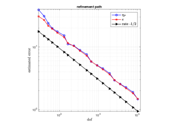
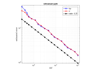
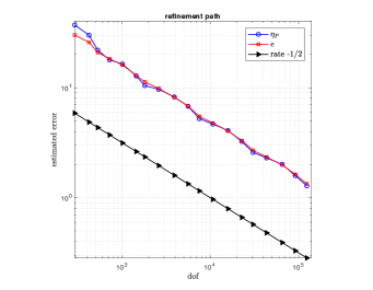
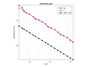
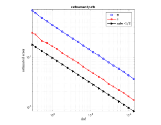
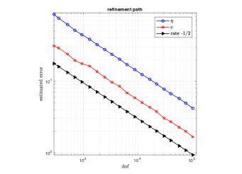
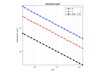
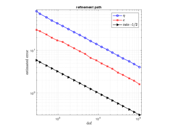
Figure 1: Exact ($e$) and estimated (using the local Poisson estimator $\eta_{P}$) energy errors computed using adaptive meshes, for Herrmann (top) and Hydrostatic (bottom) formulations of test problem 1, with $\mu=100$ and $\nu=0.4$ (left); $\mu=100$ and $\nu=0.49999$ (right).

Figure 2: Exact ($e$) and estimated (using the residual estimator $\eta$) energy errors computed using adaptive meshes, for Herrmann (top) and Hydrostatic (bottom) formulations of test problem 1, with $\mu=100$ and $\nu=0.4$ (left); $\mu=100$ and $\nu=0.49999$ (right).

5.2 A nonsmooth solution

The second test problem is taken from Ref. wihler2004locking. Again, $\Omega=(0,1)\times(0,1)$ but now $\bm{f}=\bm{0}$ and we impose the condition $\bm{u}=(g,0)^{\top}$ on $\partial\Omega$, where

$$g=\Big{\{}\begin{array}[]{lc}(1-4(x-\frac{1}{2})^{2})^{\frac{1}{2}+\alpha},&\mbox{on }\;[0,1]\times\{1\},\\ 0,&\hbox{elsewhere on }\partial\Omega.\end{array}$$

If $\alpha\in(0,\frac{1}{2})$, then the displacement exhibits $H^{\frac{3}{2}+\alpha}$–regularity. Specifically, there are singularities at the top two corners of the domain. We set the specific value $\alpha=0.1$ so that $\bm{u}\in{{\color[rgb]{0,0,0}\bm{H}^{1.6}}}(\Omega)$. This lack of smoothness is reflected in the convergence behaviour of the estimated energy error. Results obtained with the Poisson estimator $\eta_{P}$ on uniformly refined meshes are shown in Figure 4. Our results suggest that for both the Herrmann and Hydrostatic formulations, the error converges to zero at the anticipated suboptimal rate (${{\color[rgb]{0,0,0}r=0.3}}$). However, when we use adaptively refined meshes, for both the Herrmann and Hydrostatic formulations, we recover the optimal convergence rate of $r=1/2$, as shown in Figure 4. Starting from an initial mesh with $N_{0}=1,090$ degrees of freedom, the singular solution behaviour is detected and strong refinement occurs near the top corners. Figure 5 shows the meshes that are generated at the first refinement step where $N_{\ell}\geq 10^{4}$.

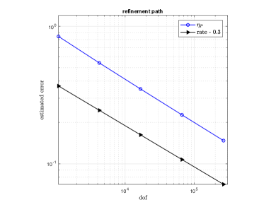
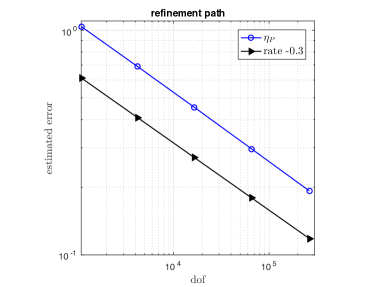
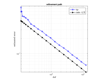
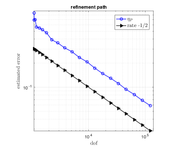
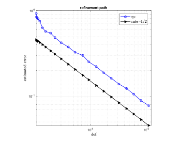
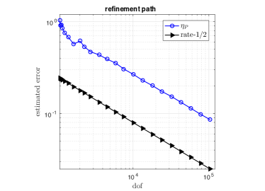
Figure 3: Estimated energy errors (using the estimator $\eta_{P}$) computed with uniform meshes, for Herrmann (left) and Hydrostatic (right) formulations of test problem 2 with $\mu=1,\nu=0.4$.

Figure 4: Estimated energy errors (using $\eta_{P}$) computed using adaptive meshes, for Herrmann (top) and Hydrostatic (bottom) formulations of test problem 2 with $\mu=1$ and $\nu=0.4$ (left); $\mu=1$ and $\nu=0.49999$ (right).

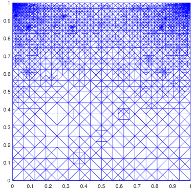
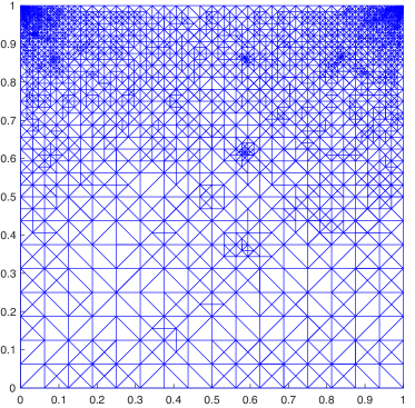
Figure 5: Adaptive meshes generated using $\eta_{P}$ for Herrmann (left) and Hydrostatic (right) formulations of test problem 2 with $\nu=0.49999$. $N_{\ell}=12,762$ (left), and $N_{\ell}=11,846$ (right).

5.3 A singular solution

To conclude, we discuss a test problem that is considered in Refs. CJ and wihler2004locking. The problem is posed in an L-shaped domain $\Omega=(-1,1)\times(-1,1)\setminus(-1,0]\times(-1,0]$. In polar coordinates, the exact displacement is

$$\bm{u}=\frac{r^{\alpha}}{2\mu}\left(\begin{array}[]{c}-(\alpha+1)\cos((\alpha+1)\phi)+(C_{2}-\alpha+1)C_{1}\cos((\alpha-1)\phi)\\ (\alpha+1)\sin((\alpha+1)\phi)+(C_{2}+\alpha-1)C_{1}\sin((\alpha-1)\phi)\end{array}\right),$$

where $\alpha=0.544483736782$ is a positive solution of $\alpha\sin(\omega)+\sin(2\omega\alpha)=0$ with

$$\omega=\frac{3\pi}{4},\quad C_{1}=-\frac{\cos((\alpha+1)\omega)}{\cos((\alpha-1)\omega)},\quad C_{2}=\frac{2(\lambda+2\mu)}{\lambda+\mu}.$$

The body force is $\bm{f}=\bm{0}$ and the nonzero essential boundary data $\bm{g}$ is represented by the piecewise linear interpolant of the given solution. Note that $\int_{\partial\Omega}\bm{g}\cdot\bm{n}\,ds\neq 0$. To compute the Lamé constants $\lambda$ and $\mu$, we choose $E=10^{5}$ and set $\nu=0.4$ or $0.49999$. Note that the exact displacement $\bm{u}$ is analytic inside the domain $\Omega$ but $\nabla\bm{u}$ is singular at the origin, so $\bm{u}\notin\bm{H}^{2}(\Omega)$. This lack of smoothness is reflected in the convergence behaviour of the estimated energy error. Results computed with the Poisson estimator $\eta_{P}$ on uniform meshes are shown in Figure 7. As in the second test problem, we observe the estimated errors converge at a suboptimal rate (here $r\approx 0.27$). Moreover, when we use adaptively refined meshes, we recover the optimal rate of convergence of $r=0.5$. This is shown in Figure 7. The singular solution behaviour is detected and strong refinement is generated around the re-entrant corner. While the effectivity indices in Figure 7 are not quite as impressive as those in Figure 2 they remain close to unity (approximately 1.35 when $\nu=0.4$ and 1.6 when $\nu=0.49999$). We infer from these results that $\eta_{P}$ provides an efficient and reliable error estimate for both Herrmann and Hydrostatic formulations.

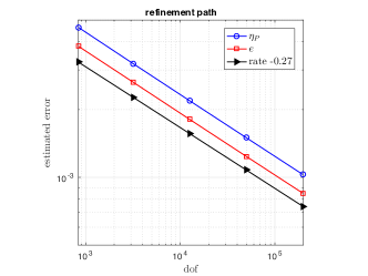
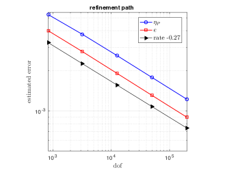
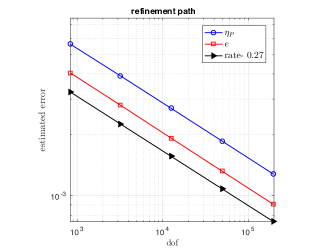
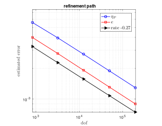
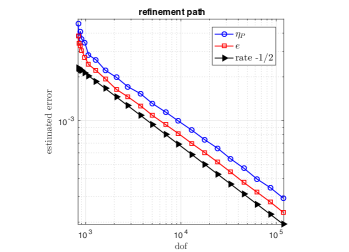
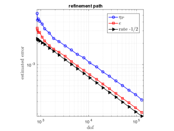
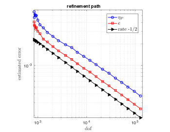
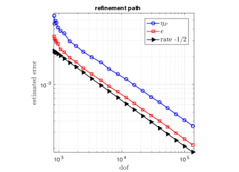
Figure 6: Estimated energy errors (using $\eta_{P}$) computed with uniform meshes for Herrmann (top) and Hydrostatic (bottom) formulations of test problem 3 with $\nu=0.4$ (left); $\nu=0.49999$ (right).

Figure 7: Estimated energy errors (using $\eta_{P}$) computed with adaptive meshes for Herrmann (top) and Hydrostatic (bottom) formulations of test problem 3 with $\nu=0.4$ (left); $\nu=0.49999$ (right).

6 Concluding remarks

There are two important contributions in this paper. First, we have developed a low-order mixed finite element method for computing locking-free approximations of linear elasticity problems. The method is computationally cheap and challenges the conventional wisdom that it is necessary to start from an inf-sup stable pair of finite element spaces. The stabilisation term is weighted by the problem specific factor of $1/2\mu$ but is otherwise parameter-free. Our a priori error analysis shows that the method provides a robust approximation of the energy error. That is, the constants in the error bounds do not depend on the Lamé coefficients. Second, we have described a practical error estimation strategy—based on solving uncoupled Poisson problems for each displacement component—that give effectivity indices that are close to unity in all cases that have been tested. Ensuring robustness in the error estimation process is fundamentally important when solving problems with large variability in the measurement of material parameters. Extending this work to enable the adaptive solution of elasticity problems with uncertain material parameters is the subject of ongoing research.

References

- [1] Mark Ainsworth and J. Tinsley Oden. A Posteriori Error Estimation in Finite Element Analysis. Wiley, 2000.
- [2] Gabriel Barrenechea and Frédéric Valentin. Consistent local projection stabilized finite element methods. SIAM J. Numer. Anal, 48(5):1801–1825, 2010.
- [3] Daniele Boffi, Franco Brezzi, and Michel Fortin. Mixed Finite Element Methods and Applications. Springer, Heidelberg, 2013.
- [4] Daniele Boffi and Rolf Stenberg. A remark on finite element schemes for nearly incompressible elasticity. Computers and Mathematics with Applications, 74(9):2047–2055, 2017.
- [5] Erik Burman and Miguel Fernández. Galerkin finite element methods with symmetric pressure stabilization for the transient Stokes equations: stability and convergence analysis. SIAM J. Numer. Anal, 47(1):409–439, 2008.
- [6] Carsten Carstensen and Joscha Gedicke. Robust residual-based a posteriori Arnold–Winther mixed finite element analysis in elasticity. Comput. Methods Appl. Mech. Engrg, 300:245–264, 2016.
- [7] P. Clément. Approximation by finite element functions using local regularization. R.A.I.R.O. Anal. Numér., 2:77–84, 1975.
- [8] Clark Dohrmann and Pavel Bochev. A stabilized finite element method for the Stokes problem based on polynomial pressure projections. Int. J. Numer. Meth. Fluids, 46:183–201, 2004.
- [9] Willy Dörfler. A convergent adaptive algorithm for Poisson’s equation. SIAM J. Numer. Anal., 33(3):1106–1124, 1996.
- [10] Howard Elman, David Silvester, and Andy Wathen. Finite Elements and Fast Iterative Solvers: with Applications in Incompressible Fluid Dynamics. Oxford University Press, Oxford, UK, 2014. Second Edition, xiv+400 pp. ISBN: 978-0-19-967880-8.
- [11] Leonard R. Herrmann. Elasticity equations for incompressible and nearly incompressible materials by a variational theorem. AIAA J., 3:1896–1900, 1965.
- [12] Paul Houston, Dominik Schötzau, and Thomas P. Wihler. An hp-adaptive mixed discontinuous Galerkin FEM for nearly incompressible linear elasticity. Comput. Methods Appl. Mech. Engrg, 195:3224–3246, 2006.
- [13] Thomas J. R. Hughes. The Finite Element Method. Prentice-Hall, New Jersey, 1987.
- [14] David Kay and David Silvester. A posteriori error estimation for stabilized mixed approximations of the Stokes equations. SIAM J. Sci. Comput., 21:1321–1336, 1999.
- [15] Nasserdine Kechkar and David Silvester. Analysis of locally stabilized mixed finite element methods for the Stokes problem. Math. Comput., 58:1–10, 1992.
- [16] A. Khan, C. E. Powell, and D. J. Silvester. Robust a posteriori error estimators for mixed approximation of nearly incompressible elasticity. arXiv eprint, October 2017. https://arxiv.org/abs/1710.03328.
- [17] Reijo Kouhia and Rolf Stenberg. A linear nonconforming finite element method for nearly incompressible elasticity and Stokes flow. Comput. Methods Appl. Mech. Engrg, 124(3):195–212, 1995.
- [18] Sean Norburn and David Silvester. Stable vs. stabilised mixed methods for incompressible flow. Comput. Methods Appl. Mech. Engrg, 166:131–141, 1998.
- [19] David Silvester, Alex Bespalov, Qifeng Liao, and Leonardo Rocchi. Triangular IFISS (TIFISS) version 1.1., March 2017. http://www.manchester.ac.uk/ifiss/tifiss.
- [20] Rudiger Verfürth. A Posteriori Error Estimation Techniques for Finite Element Methods. Oxford University Press, Oxford, 2013.
- [21] Thomas P Wihler. Locking-free DGFEM for elasticity problems in polygons. IMA J. Numer. Anal., 24(1):45–75, 2004.