A Game Theoretic Approach to
Hyperbolic Consensus Problems

Abstract

We introduce the use of conservation laws to develop strategies in multi-player consensus games. First, basic well posedness results provide a reliable analytic setting. Then, a general non anticipative strategy is proposed through its rigorous analytic definitions and then tested by means of numerical integrations.

Keywords: Hyperbolic Consensus Model, Multi-agent Consensus Control, Conservation Laws

2010 MSC: 91A23, 35L65, 70F45

1 Introduction

A group of “leaders”, or broadcasting agents, aims at getting the consensus of a variety of individuals. We identify each individual’s opinion with a “position” $x$ moving in ${\mathbb{R}}^{N}$. It is then natural to describe the leaders through their ”positions” $P_{1},P_{2},\ldots,P_{k}$, also in ${\mathbb{R}}^{N}$. We are thus lead to the general system of ordinary differential equation

$$\left\{\begin{array}[]{l}\dot{x}=v\left(t,x,P_{1}(t),\ldots,P_{k}(t)\right)\\ x(0)=\bar{x}\end{array}\right.$$

$t$ being time. The vector field $v$ describes the interaction among individuals and agents, which can be attractive, repulsive, or a mixture of the two. Clearly, no linearity assumption can be reasonably required on $v$, otherwise the interaction between an agent and the individuals increases as the distance between them increases.

The task of the agent $P_{i}$, be it attractive or repulsive, is to maximize its own consensus, i.e., to drive the maximal amount of individuals (or their opinions) as near as possible to its own target region $\mathcal{T}_{i}$ at time $T$, for a suitable non empty region $\mathcal{T}_{i}\subset{\mathbb{R}}^{N}$. The time horizon $T$ is finite and the same for all agents.

A high number of individuals, as well as uncertainties in their initial positions or specific movements, suggests to describe the dynamics underneath the present problem through the continuity equation

$$\partial_{t}\rho+\mathinner{\mathop{\rm div}}_{x}\left(\rho\;v\left(t,x,P_{1}(t),\ldots,P_{k}(t)\right)\right)=0\,,$$ (1.1)

where the description of each individual is substituted by that of the individuals’ density distribution $\rho=\rho(t,x)$, while the goal of the $i$–th leader is formalized through the minimization of the quantity

$$\mathcal{J}_{i}=\int_{{\mathbb{R}}^{N}}\rho(T,x)\;d(x,\mathcal{T}_{i})\,\mathinner{\mathrm{d}{x}}$$ (1.2)

where $d(x,\mathcal{T}_{i})=\inf_{y\in\mathcal{T}_{i}}{\left\|x-y\right\|}$ is the distance between the position $x$ and the target $\mathcal{T}_{i}$.

Aim of this paper is to formalize the above setting, to provide basic well posedness theorems and to initiate the search for controls/strategies to tackle the above problem. Note that the case $k=1$ of a single broadcasting agent leads to a control problem, while the case $k>1$ of $k$ possibly competing agents fits into game theory.

As it is usual in control theory, rather than the agents’ positions $P_{i}$, it is preferable to use as controls/strategies the agents’ speeds $u_{i}$, with $u_{i}\in{\mathbb{R}}^{N}$, subject to a boundedness constraint of the type ${\left\|u_{i}\right\|}\leq U$, for a positive $U$. Introducing the initial individuals’ distribution $\bar{\rho}$ and agents’ positions $\bar{P}_{1},\ldots,\bar{P}_{k}$, the dynamics is then described by the Cauchy Problem

$$\left\{\begin{array}[]{l}\partial_{t}\rho+\mathinner{\mathop{\rm div}}_{x}\left(\rho\;v\!\left(t,x,P_{1}(t),\ldots,P_{k}(t)\right)\right)=0\\ \rho(0,x)=\bar{\rho}(x)\end{array}\right.\;\mbox{ where }\;\left\{\begin{array}[]{l}\dot{P}_{i}=u_{i}(t)\\ P_{i}(0)=\bar{P}_{i}\end{array}\right.\quad i=1,\ldots,k$$ (1.3)

where the cost functionals $\mathcal{J}_{i}$ are as in (1.2). This structure is amenable to the introduction of several control/game theoretic concepts, from optimal controls to Nash equilibria, and to the search for their existence. Below we initiate this study providing the basic analytic framework and tackling the problem of control/strategies to minimize costs of the type (1.2). Various numerical integrations illustrate the rigorous results obtained.

Note that the present setting, restricted to the case $N=2$, allows also to describe the individual–continuum interactions considered, for instance, in [8], see also [6, 7], and [9] where an entirely different analytic framework is exploited. From this point of view, the present work is related to the vast literature on crowd and swarm dynamics, see the recent works [4, 5, 11, 14, 15, 16, 18] or the review [1] and the references therein.

Concerning our choice of the conservation law (1.1), we stress that typical of equations of this kind is the finite speed both of propagation of information and of the support of the density. This is in contrast with the typical situation in standard differential games ruled by parabolic equations.

In the next section we first provide the basic notation and definitions, then we provide basic well posedness results and introduce a reasonable non anticipative strategy. Section 3 is devoted to sample applications, while all analytic proofs are deferred to Section 4.

2 Analytic Results

Throughout, the positive time $T$ and the maximal speed $U$ are fixed. For $a,b\in{\mathbb{R}}$, denote $\langle a,b\rangle=[\min\{a,b\},\max\{a,b\}]$. By $\mathcal{L}^{N}$ we mean the Lebesgue measure in ${\mathbb{R}}^{N}$. The open, respectively closed, ball in ${\mathbb{R}}^{m}$ centered at $u$ with radius $U$ is $B_{{\mathbb{R}}^{m}}(u,U)$, respectively $\overline{B_{{\mathbb{R}}^{m}}(u,U)}$; when the space is clear, we shorten to $B(u,U)$ or $\overline{B(u,U)}$. In ${\mathbb{R}}$, ${\left|\,\cdot\,\right|}$ is the absolute value, while ${\left\|\,\cdot\,\right\|}$ is the Euclidean norm in ${\mathbb{R}}^{N}$. The norm in the functional space $\mathcal{F}$ is denoted ${\left\|\,\cdot\,\right\|}_{\mathcal{F}}$. The space $\mathbf{C^{0}}(A;{\mathbb{R}}^{n})$ of the ${\mathbb{R}}^{n}$-valued functions defined on the subset $A$ of ${\mathbb{R}}^{m}$ is equipped with the norm ${\left\|f\right\|}_{\mathbf{C^{0}}(A;{\mathbb{R}}^{n})}=\sup_{x\in A}{\left\|f(x)\right\|}$. Throughout, $\mathop{\mathrm{missing}}{TV}(\,\cdot\,)$ stands for the total variation, see [10, Chapter 5]. For a measurable function $\rho$ defined on ${\mathbb{R}}^{N}$, $\mathop{\mathrm{missing}}{spt}\rho$ is its support, see [3, Proposition 4.17].

Introduce $P\equiv(P_{1},\ldots,P_{k})$, so that $P\in{\mathbb{R}}^{m}$ with $m=k\,N$, and rewrite (1.3) as

$$\left\{\begin{array}[]{l}\partial_{t}\rho+\mathinner{\mathop{\rm div}}_{x}\left(\rho\;v\!\left(t,x,P(t)\right)\right)=0\\ \rho(0,x)=\bar{\rho}(x)\end{array}\right.\quad\mbox{ where }\quad\left\{\begin{array}[]{l}\dot{P}=u(t)\\ P(0)=\bar{P}\,.\end{array}\right.$$ (2.1)

Below, recurrent assumptions on the function $v$ in (2.1) are the following:

(v0):

The vector field $v\in\mathbf{C^{0}}([0,T]\times{\mathbb{R}}^{N}\times{\mathbb{R}}^{m};{\mathbb{R}}^{N})$ is such that for all $t\in[0,T]$ and $P\in{\mathbb{R}}^{m}$, the map $x\to v(t,x,P)$ is in $\mathbf{C^{0,1}}({\mathbb{R}}^{N};{\mathbb{R}}^{N})$.

(v1):

(v0) holds and moreover

• for all $t\in[0,T]$ and $P\in{\mathbb{R}}^{m}$, the map $x\to v(t,x,P)$ is in $\mathbf{C^{1,1}}({\mathbb{R}}^{N};{\mathbb{R}}^{N})$;

• for all $t\in[0,T]$ and $x\in{\mathbb{R}}^{N}$, the map $P\to v(t,x,P)$ is in $\mathbf{C^{0,1}}({\mathbb{R}}^{m};{\mathbb{R}}^{N})$.

We now prove well posedness and basic estimates for (1.3) or, equivalently, (2.1).

Proposition 2.1.

Fix positive $T$ and $U$. Let $v$ satisfy (v0). For any $\bar{\rho}\in\mathbf{L^{1}}({\mathbb{R}}^{N};{\mathbb{R}})$, $\bar{P}\in{\mathbb{R}}^{m}$ and $u\in\mathbf{L^{\infty}}([0,T];\overline{B_{{\mathbb{R}}^{m}}(0,U)})$, problem (2.1) admits the unique solution

$$\rho(t,x)=\bar{\rho}\left(X(0;t,x)\right)\exp\left(-\int_{0}^{t}\mathinner{\mathop{\rm div}}_{x}v\left(\tau,X(\tau;t,x),P(\tau)\right)\mathinner{\mathrm{d}{\tau}}\right)$$

where $t\to X(t;\bar{t},\bar{x})$ solves $\left\{\begin{array}[]{l@{}}\dot{x}=v\left(t,x,P(t)\right)\\ x(\bar{t})=\bar{x}\end{array}\right.$ and $\displaystyle P(t)=\bar{P}+\int_{0}^{t}u(\tau)\mathinner{\mathrm{d}{\tau}}$ for $t\in[0,T]$. Moreover, if $v$ satisfies (v1) and $u_{1},u_{2}\in\mathbf{L^{\infty}}([0,T];\overline{B_{{\mathbb{R}}^{m}}(0,U)})$, then (with obvious notation) for all $t\in[0,T]$,

$${\left\|X_{1}(t;0,\bar{x})-X_{2}(t;0,\bar{x})\right\|} \leq C\,t\,e^{C\,t}\;{\left\|P_{1}-P_{2}\right\|}_{\mathbf{C^{0}}([0,t];{\mathbb{R}}^{m})}$$ (2.2)

$${\left\|\rho_{1}(t)-\rho_{2}(t)\right\|}_{\mathbf{L^{1}}({\mathbb{R}}^{N};{\mathbb{R}})} \leq C\,\Bigl{(}{\left\|\mathinner{\mathop{\rm grad}}_{x}\bar{\rho}\right\|}_{\mathbf{L^{\infty}}({\mathbb{R}}^{N};{\mathbb{R}}^{N})}\;\mathcal{L}^{N}\!\left(B(\mathop{\mathrm{missing}}{spt}\bar{\rho},Cte^{Ct})\right)$$

$$\qquad\qquad+{\left\|\bar{\rho}\right\|}_{\mathbf{L^{1}}({\mathbb{R}}^{N};{\mathbb{R}})}\,(1+C\,t)\Bigr{)}t\,e^{2Ct}\,{\left\|P_{1}-P_{2}\right\|}_{\mathbf{C^{0}}([0,t];{\mathbb{R}}^{m})}$$

where $C$ is independent of the initial datum, more precisely:

$$C=\max\left\{\begin{array}[]{ll}{\left\|v\right\|}_{\mathbf{L^{\infty}}([0,t]\times{\mathbb{R}}^{N}\times{\mathbb{R}}^{m};{\mathbb{R}}^{N})},&{\left\|D_{x}v\right\|}_{\mathbf{L^{\infty}}([0,t]\times{\mathbb{R}}^{N}\times{\mathbb{R}}^{m};{\mathbb{R}}^{N\times N})},\\ {\left\|D_{P}v\right\|}_{\mathbf{L^{\infty}}([0,t]\times{\mathbb{R}}^{N}\times{\mathbb{R}}^{m};{\mathbb{R}}^{N\times m})},&{\left\|\mathinner{\mathop{\rm grad}}_{x}\mathinner{\mathop{\rm div}}_{x}v\right\|}_{\mathbf{L^{\infty}}([0,t]\times{\mathbb{R}}^{N}\times{\mathbb{R}}^{m};{\mathbb{R}}^{N})}\end{array}\right\}\,.$$ (2.4)

The proof is deferred to Section 4. Here, the term “solution” means Kružkov solution [12, Definition 1], which is also a strong solution as soon as $\bar{\rho}$ is smooth. A straightforward consequence of the above Lemma is the following convergence result, which we state without proof.

Corollary 2.2.

Fix positive $T$ and $U$. Let $v$ be bounded and satisfy (v1), $\bar{\rho}\in\mathbf{L^{1}}({\mathbb{R}}^{N};{\mathbb{R}})$ and $\bar{P}\in{\mathbb{R}}^{m}$. If $u_{n},u_{*}\in\mathbf{L^{\infty}}([0,T];\overline{B_{{\mathbb{R}}^{m}}(0,U)})$ are such that $u_{n}\mathinner{\stackrel{{\scriptstyle\star}}{{\rightharpoonup}}}u_{*}$ in $\mathbf{L^{\infty}}([0,T];{\mathbb{R}}^{m})$ as $n\to+\infty$, then, up to a subsequence,

$$P_{n}\to P_{*}\mbox{ in }\mathbf{C^{0}}([0,T];{\mathbb{R}}^{N})\quad\mbox{ and }\quad\begin{array}[]{r@{\;}c@{\;}l@{\mbox{ in }}l}\rho_{n}(t)&\to&\rho_{*}(t)&\mathbf{L^{1}}({\mathbb{R}}^{N};{\mathbb{R}})\mbox{ for all }t\in[0,T]\,,\\ \rho_{n}&\to&\rho_{*}&\mathbf{C^{0}}\left([0,T];\mathbf{L^{1}}({\mathbb{R}}^{N};{\mathbb{R}})\right)\,.\end{array}$$

If $\bar{\rho}\in\mathbf{C^{1}}({\mathbb{R}}^{N};{\mathbb{R}})$, then $\begin{array}[]{rcll}\mathinner{\mathop{\rm grad}}_{x}\rho_{n}(t)&\to&\mathinner{\mathop{\rm grad}}_{x}\rho_{*}(t)&\mbox{ in }\mathbf{L^{1}}({\mathbb{R}}^{N};{\mathbb{R}})\mbox{ for all }t\in[0,T]\\ \mathinner{\mathop{\rm grad}}_{x}\rho_{n}&\to&\mathinner{\mathop{\rm grad}}_{x}\rho_{*}&\mbox{ in }\mathbf{C^{0}}\left([0,T];\mathbf{L^{1}}({\mathbb{R}}^{N};{\mathbb{R}})\right)\end{array}$.

The $i$-th leader $P_{i}$ seeks a control $u_{i}\in\mathbf{L^{\infty}}\big{(}[0,T];\overline{B(0,U)}\big{)}$ that minimizes the cost $\mathcal{J}_{i}=\int_{{\mathbb{R}}^{N}}\rho(T,x)\,\psi(x)\,\mathinner{\mathrm{d}{x}}$, which reduces to (1.2) in the case $\psi(x)=d(x,\mathcal{T}_{i})$. Assume first that $P_{i}$ knows in advance the strategies $u_{j}$, for $j\neq i$, of the other controllers $P_{j}$, so that its task amounts to minimize (2.5). Corollary 2.2 ensures that

$$\begin{array}[]{ccccc}\mathcal{J}_{i}&\colon&\mathbf{L^{\infty}}\left([0,T];\overline{B(0,U)}\right)&\to&{\mathbb{R}}\\ &&u_{i}&\to&\displaystyle\int_{{\mathbb{R}}^{N}}\rho(T,x)\,\psi(x)\,\mathinner{\mathrm{d}{x}}\end{array}$$ (2.5)

is weak$\star$ continuous. Hence, by the weak$\star$ compactness of $\mathbf{L^{\infty}}([0,T];\overline{B(0,U)})$, there exists an optimal control $u_{i}^{*}$ that minimizes $\mathcal{J}_{i}$.

Note however that this approach can hardly be used in a game theoretic setting, since it requires that $P_{i}$ is aware of all other strategies $u_{j}$, $j\neq i$, on the whole time interval $[0,T]$, which is unreasonable whenever different agents are competing.

We now proceed towards the definition of a non anticipative strategy. To this aim, we simplify the notation setting $P=P_{i}$, $u=u_{i}$, $\mathcal{J}=\mathcal{J}_{i}$ and comprising within the time dependence of the function $v$ all the other strategies $u_{j}$, for $j\neq i$. In this setting, we define a non anticipative strategy $u$ for the controller $P$, i.e., a strategy $u=u(t)$ that depends only on $\rho$ at times $s\in\left[0,t\right[$.

For a positive (suitably small) $\Delta t$, we seek the best choice of a speed $w\in\overline{B(0,U)}$ on the interval $[t,t+\Delta t]$ such that the solution $\rho_{w}=\rho_{w}(\tau,x)$ to

$$\left\{\begin{array}[]{l}\partial_{\tau}\rho_{w}+\mathinner{\mathop{\rm div}}_{x}\left(\rho_{w}\;v\!\left(t,x,P(t)+(\tau-t)w\right)\right)=0\\ \rho_{w}(t,x)=\rho(t,x)\end{array}\right.\qquad\tau\in[t,t+\Delta t]$$ (2.6)

is likely to best contribute to decrease the value of $\mathcal{J}$. Remark that the dependence of $v$ on $t$ in (2.6) is frozen at time $t$. It is this choice that will later lead to a non anticipative strategy.

We now verify that (2.6) is well posed.

Lemma 2.3.

Fix positive $T$, $U$, and $\Delta t\in]0,T[$. Let $v\in\mathbf{C^{0,1}}([0,T]\times{\mathbb{R}}^{N}\times{\mathbb{R}}^{N};{\mathbb{R}}^{N})$. For any $\bar{\rho}\in\mathbf{L^{1}}({\mathbb{R}}^{N};{\mathbb{R}})$, $\bar{P}\in{\mathbb{R}}^{N}$, $u\in\mathbf{L^{\infty}}([0,T];\overline{B(0,U)})$, $t\in\left[0,T-\Delta t\right[$ and $w\in{\mathbb{R}}^{N}$, problem (2.6) admits a unique solution given by

$$\rho_{w}(\tau,x)=\rho\left(t,X_{t,w}(t;\tau,x)\right)\;\exp\left(-\int_{t}^{\tau}\mathinner{\mathop{\rm div}}_{x}v\left(t,X_{t,w}(s;\tau,x),P(t)+(s-t)\,w\right)\mathinner{\mathrm{d}{s}}\right)$$ (2.7)

where

$$\tau\to X_{t,w}(\tau;\bar{t},x)\quad\mbox{ solves }\quad\left\{\begin{array}[]{l}\xi^{\prime}=v\left(t,\xi,P(t)+(\tau-t)w\right)\\ \xi(\bar{t})=x\end{array}\right.\mbox{ for }\bar{t},\tau\in[t,t+\Delta t]\,.$$ (2.8)

Moreover, if $\bar{\rho}\in\mathbf{C^{1,1}}({\mathbb{R}}^{N};{\mathbb{R}})$ and $\mathcal{L}^{N}(\mathop{\mathrm{missing}}{spt}\bar{\rho})<+\infty$, for all $w_{1},w_{2}\in{\mathbb{R}}^{N}$

$$\begin{array}[]{rcl}&&{\left\|\rho_{w_{1}}(t+\Delta t)-\rho_{w_{2}}(t+\Delta t)\right\|}_{\mathbf{L^{1}}({\mathbb{R}}^{N};{\mathbb{R}})}\\ &\leq&\left({\left\|\mathinner{\mathop{\rm grad}}_{x}\bar{\rho}\right\|}_{\mathbf{L^{\infty}}({\mathbb{R}}^{N};{\mathbb{R}}^{N})}\;\mathcal{L}^{N}\left(\mathop{\mathrm{missing}}{spt}\bar{\rho},Ce^{C\Delta t}\Delta t\right)+(1+C\,\Delta t){\left\|\bar{\rho}\right\|}_{\mathbf{L^{1}}({\mathbb{R}}^{N};{\mathbb{R}})}\right)\\ &&\quad\times Ce^{2C\Delta t}\,(\Delta t)^{2}\,{\left\|w_{1}-w_{2}\right\|}\end{array}$$ (2.9)

where

$$C=\max\left\{\begin{array}[]{l}{\left\|v\right\|}_{\mathbf{L^{\infty}}([t,t+\Delta t]\times{\mathbb{R}}^{N}\times B(P(t),\Delta t\,U);{\mathbb{R}}^{N})},\\ {\left\|D_{x}v\right\|}_{\mathbf{L^{\infty}}([t,t+\Delta t]\times{\mathbb{R}}^{N}\times B(P(t),\Delta t\,U);{\mathbb{R}}^{N\times N})},\\ \frac{1}{2}\;{\left\|D_{P}v\right\|}_{\mathbf{L^{\infty}}([t,t+\Delta t]\times{\mathbb{R}}^{N}\times{\mathbb{R}}^{N};{\mathbb{R}}^{N\times N})},\\ {\left\|D_{P}\mathinner{\mathop{\rm div}}_{x}v\right\|}_{\mathbf{L^{\infty}}([t,t+\Delta t]\times{\mathbb{R}}^{N}\times{\mathbb{R}}^{N};{\mathbb{R}}^{N})}\end{array}\right\}$$ (2.10)

(Above and in the sequel, $\xi^{\prime}=\frac{\mathinner{\mathrm{d}{\xi}}}{\mathinner{\mathrm{d}{\tau}}}$). The proof of Lemma 2.3 is deferred to Section 4.

In the case of the functional (1.2), a natural choice for the agent $P$ at time $t$ is then to choose a speed $w$ on the time interval $[t,t+\Delta t]$ to minimize the quantity

$$\mathcal{J}_{t,\Delta t}(w)=\int_{{\mathbb{R}}^{N}}\rho_{w}(t+\Delta t,x)\;\psi(x)\,\mathinner{\mathrm{d}{x}}\,.$$ (2.11)

Proposition 2.4.

Fix positive $T,U$, $\Delta t\in]0,T[$, and fix a boundedly supported initial datum $\bar{\rho}\in\mathbf{L^{1}}({\mathbb{R}}^{N};{\mathbb{R}})$, $\bar{P}\in{\mathbb{R}}^{N}$, a speed law $v\in\mathbf{C^{0,1}}([0,T]\times{\mathbb{R}}^{N}\times{\mathbb{R}}^{N};{\mathbb{R}}^{N})$ and a weight $\psi\in\mathbf{L^{\infty}}({\mathbb{R}}^{N};{\mathbb{R}})$. Then, with the notation in (2.1) and (2.6), for any $t\in\left[0,T\right[$ and $\Delta t\in\left]0,T-t\right]$ the map

$$\begin{array}[]{ccccc}\mathcal{J}_{t,\Delta t}&\colon&{\mathbb{R}}^{N}&\to&{\mathbb{R}}\\ &&w&\to&\displaystyle\int_{{\mathbb{R}}^{N}}\rho_{w}(t+\Delta t,x)\;\psi(x)\mathinner{\mathrm{d}{x}}\end{array}$$

is well defined and Lipschitz continuous.

The main theorem now follows, providing explicit information on a non anticipative optimal choice of $w$.

Theorem 2.5.

Fix positive $T$, $U$, and $\Delta t\in]0,T[$. Let $v\in\mathbf{C^{2}}([0,T]\times{\mathbb{R}}^{N}\times{\mathbb{R}}^{N};{\mathbb{R}}^{N})$, $\psi\in\mathbf{L^{\infty}}({\mathbb{R}}^{N};{\mathbb{R}})$ and a boundedly supported $\bar{\rho}\in\mathbf{C^{1}}({\mathbb{R}}^{N};{\mathbb{R}})$. Define $\rho$ as the solution to (2.1) and $\rho_{w}$ as the solution to (2.6), for a $w\in{\mathbb{R}}^{N}$. The map

$$\begin{array}[]{ccccc}\mathcal{J}_{t,\Delta t}&\colon&{\mathbb{R}}^{N}&\to&{\mathbb{R}}\\ &&w&\to&\displaystyle\int_{{\mathbb{R}}^{N}}\rho_{w}(t+\Delta t,x)\;\psi(x)\mathinner{\mathrm{d}{x}}\end{array}$$ (2.12)

admits the expansion

$$\mathcal{J}_{t,\Delta t}(w+\delta_{w})=\mathcal{J}_{t,\Delta t}(w)+\mathinner{\mathop{\rm grad}}_{w}\mathcal{J}_{t,\Delta t}(w)\cdot\delta_{w}+o(\delta_{w})\qquad\mbox{ as }w\to 0$$ (2.13)

where, as $\Delta t\to 0$,

$$\begin{array}[]{@{}r@{\;}c@{\;}l@{}}\!\!\!\!\!\!\mathinner{\mathop{\rm grad}}_{w}\mathcal{J}_{t,\Delta t}(w)\!&=\!&\displaystyle\dfrac{(\Delta t)^{2}}{2}\!\!\!\int_{{\mathbb{R}}^{N}}\!\!\Big{[}\!\mathinner{\mathop{\rm grad}}_{x}\rho(t,x)D_{P}v\!\left(t,x,P(t)\right)\!\!-\!\!\rho(t,x)\mathinner{\mathop{\rm grad}}_{P}\mathinner{\mathop{\rm div}}_{x}v\!\left(t,x,P(t)\right)\!\!\Big{]}\!\psi(x)\mathinner{\mathrm{d}{x}}\\[20.0pt] &&+o(\Delta t)^{2}.\end{array}\!\!\!\!\!\!\!\!\!\!\!\!\!\!\!\!\!\!\!\!\!\!$$ (2.14)

The proof is deferred to Section 4. On the basis of Theorem 2.5, the definition of an effective non anticipative strategy for $P_{i}$ can be easily achieved as follows. Split the interval $[0,T]$ in smaller portions $\left[t_{\ell},t_{\ell+1}\right[$, where $t_{\ell}=\ell\,\Delta t$. On each of them, define $u_{i}(t)=w_{\ell}$, where $w_{\ell}$ minimizes on $\overline{B(0,U)}$ the cost $\mathcal{J}_{t_{\ell},\Delta t}$ defined in (2.12). The leading term in the right hand side of (2.14) is independent of $w$, so that for $\Delta t$ small it is reasonable to choose

$$w_{\ell}=-\dfrac{U\displaystyle\int_{{\mathbb{R}}^{N}}\Big{[}\mathinner{\mathop{\rm grad}}_{x}\rho(t_{\ell},x)\;D_{P}v\left(t_{\ell},x,P_{i}(t_{\ell})\right)-\rho(t_{\ell},x)\;\mathinner{\mathop{\rm grad}}_{P}div_{x}v\left(t_{\ell},x,P_{i}(t_{\ell})\right)\Big{]}\psi(x)\mathinner{\mathrm{d}{x}}}{{\left\|\displaystyle\int_{{\mathbb{R}}^{N}}\Big{[}\mathinner{\mathop{\rm grad}}_{x}\rho(t_{\ell},x)\;D_{P}v\!\left(t_{\ell},x,P_{i}(t_{\ell})\right)-\rho(t_{\ell},x)\;\mathinner{\mathop{\rm grad}}_{P}\mathinner{\mathop{\rm div}}_{x}v\!\left(t_{\ell},x,P_{i}(t_{\ell})\right)\Big{]}\psi(x)\mathinner{\mathrm{d}{x}}\right\|}}$$

as long as the denominator above does not vanish, in which case we set $w_{\ell}=0$. Remark that, through the term $\rho_{\ell}$, the right hand side above depends on all the past values $w_{0},\ldots,w_{\ell-1}$ attained by $u_{i}$. Formally, in the limit $\Delta t\to 0$, the above relations thus leads to a delayed integrodifferential equation.

3 Examples

This section presents a few numerical integrations of the game (1.3)–(1.2) in which a strategy is chosen as described in Section 2.

As the function $v$ in (1.3), we choose

$$v(t,x,P)=\sum_{i=1}^{k}a_{i}\left({\left\|x-P_{i}\right\|}\right)\,\left(P_{i}-x\right)\,,$$ (3.1)

where $P\equiv(P_{1},\ldots,P_{k})$ and $a_{i}\colon{\mathbb{R}}^{+}\to{\mathbb{R}}$, $i\in\left\{1,\cdots,k\right\}$, is chosen so that (v1) holds. In other words, at time $t$, the velocity $v(t,x,P)$ of the individual at $x$ is the sum of $k$ vectors, each of them parallel to the straight line through $x$ and the agent’s position $P_{i}$ and its strength depends on the distance between $x$ and $P_{i}$. Typically, the functions $a_{i}$ is chosen so that for all $t$ and $P$, the map $x\to v(t,x,P)$ is either compactly supported, or vanishes as ${\left\|x\right\|}\to+\infty$. Note that $a_{i}>0$ whenever $P_{i}$ is attractive, while $a_{i}<0$ in the repulsive case. In the examples below, the targets are single points and, correspondingly, the cost $\psi_{i}$ is the distance from that point.

With reference to (2.1), in each of the integrations below we use the Lax–Friedrichs algorithm [13, Section 4.6] with dimensional splitting [13, Section 19.5] to integrate the conservation law, while the usual explicit forward Euler method is adequate for the ordinary differential equation. To ease the presentations of the results, we fix the space dimension $N=2$. Correspondingly, in each of the rectangular domains $\Omega$ considered below, we fix a rectangular regular grid consisting of $n_{x}\times n_{y}$ points. The treatment of the boundary $\partial\Omega$ is eased whenever the vector $v$ along $\partial\Omega$ points inward.

3.1 A Single Agent

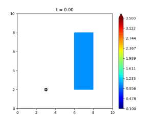
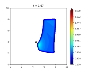
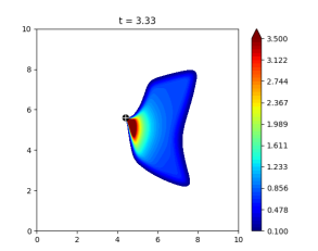
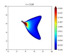
Consider (2.1) in the numerical domain $\Omega=[0,10]\times[0,10]$, with

$$\begin{array}[]{@{}r@{\;}c@{\;}l@{}}N&=&2\,,\\ k&=&1\,,\\ m&=&2\,,\end{array}\qquad\begin{array}[]{r@{\;}c@{\;}l@{}}a_{1}(\xi)&=&\frac{1}{\xi}\,e^{-\xi/10}\,,\\ v(t,x,P)&=&e^{-{\left\|x-P_{1}\right\|}/10}\,(P_{1}-x)\,,\\ U&=&3/2\end{array}\qquad\begin{array}[]{r@{\;}c@{\;}l@{}}\bar{\rho}&=&\chi_{[6,8]\times[2,8]},\\ \bar{P}_{1}&\equiv&(3,2),\end{array}\qquad\mathcal{T}_{1}=\left\{(1,8)\right\}.$$ (3.2)

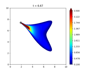
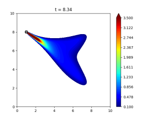
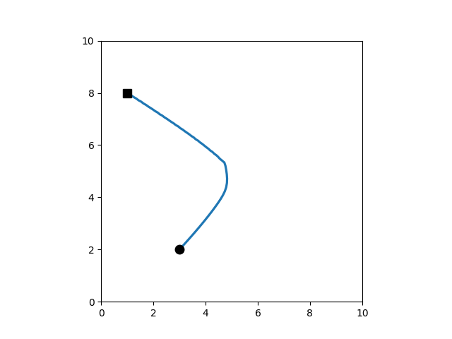
We now compute the solution to (1.3) with $u$ piecewise constant given by the strategy (2.14), constant on intervals $[j\,\Delta t,(j+1)\,\Delta t]$, where $\Delta t=1/100$. The resulting solution, obtained on a grid of $6000\times 6000$ cells, is displayed in Figure 1.

Figure 1: Numerical integration of (1.3) with the strategy (2.14) and the parameters (3.2). The first 7 figures depict the contour plots of the solution $\rho$ and the position of $P$, the bottom right diagram displays the trajectory of $P_{1}$, whose initial position is $\left(3,2\right)$, drawn as a black circle. Here, $\Delta t=1/100$. Note that, in spite of the myopic nature of the strategy (2.14), the leader first moves to the right and then turns back to the left.

Remarkably, although the strategy (2.14) is fully myopic, the leader $P_{1}$ does not move directly towards the target $\mathcal{T}_{1}$. On the contrary, it first moves to the right to collect a higher quantity of individuals and then moves back to the left; see Figure 1. The resulting cost (1.2) is $29.33$.

3.2 Two Competing Attractive Agents

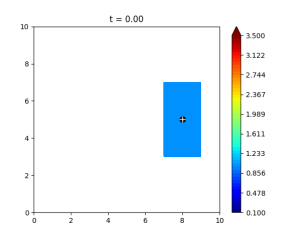
We now test the strategy (2.14) against an a priori assigned strategy. More precisely, we let $\Omega=[0,10]\times[0,10]$, with

$$\begin{array}[]{@{}r@{\;}c@{\;}l@{}}N&=&2\,,\\ k&=&2\,,\\ m&=&4\,,c\end{array}\qquad\begin{array}[]{r@{\;}c@{\;}l@{}}a_{1}(\xi)&=&\frac{1}{\xi}\,e^{-\xi/5}\,,\\ a_{2}(\xi)&=&\frac{1}{\xi}\,e^{-\xi/5}\,,\\ v(t,x,P)&=&\mbox{as in~{}\eqref{eq:velocity-simulation}}\,,\\ U&=&3/2\,,\end{array}\qquad\begin{array}[]{r@{\;}c@{\;}l@{}}\bar{\rho}&=&\chi_{[7,9]\times[3,7]},\\ \bar{P}_{1}&=&(8,5),\\ \bar{P}_{2}&=&(8,5),\end{array}\qquad\begin{array}[]{@{}r@{\;}c@{\;}l@{}}\mathcal{T}_{1}&=&\left\{(1,9)\right\},\\ \mathcal{T}_{2}&=&\left\{(1,1)\right\}.\end{array}$$ (3.3)

Moreover, we first assign to $P_{1}$ the rectilinear trajectory

$$P_{1}(t)=\left[\begin{array}[]{@{}c@{}}8\\ 5\end{array}\right]+\left[\begin{array}[]{@{}c@{}}-7/10\\ 2/5\end{array}\right]t\,,\quad\mbox{ corresponding to }\quad u_{1}(t)=\left[\begin{array}[]{@{}c@{}}-7/10\\ 2/5\end{array}\right]\,.$$ (3.4)

The agent $P_{1}$ follows a rectilinear trajectory towards the target located at the point $\left(1,9\right)$. At the final time $T=10$, the cost of player $P_{1}$, when alone, is $11.73$, see Table 1.

Figure 2: Numerical integration of (1.3)–(3.3) with two players. $P_{1}$ is assigned strategy (3.4), while $P_{2}$ uses (2.14) with $\Delta t=1/100$. The first 7 figures depict the contour plots of the solution $\rho$, the bottom right diagram displays the trajectories of $P_{1}$ and $P_{2}$, whose initial positions are as in (3.3). $P_{2}$ wins.

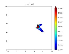
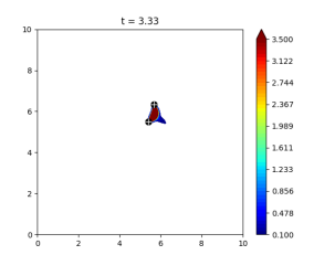
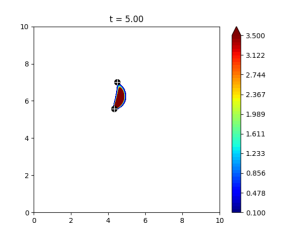
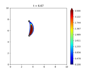
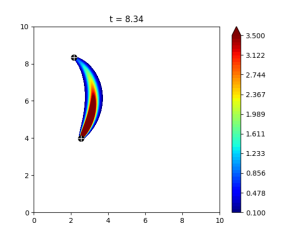
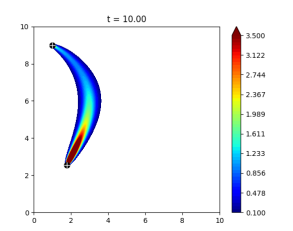
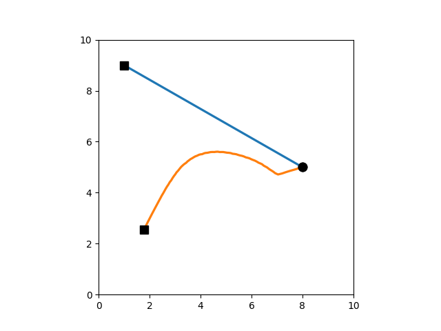
Then, we insert also the player $P_{2}$, assigning its strategy $u_{2}$ by means of (2.14). The result is shown in Figure 2: strategy (2.14) leads to the victory of $P_{2}$. Here, $P_{2}$ first moves slightly up, superimposing its attraction to that of $P_{1}$. Then, it bends downwards attracting more individuals than $P_{1}$; see Figure 2. The agent $P_{2}$ goes initially towards the target located at $\left(1,1\right)$, but, after a small amount of time, it turns up, attracting more individuals than $P_{1}$.

The results pertaining the costs $\mathcal{J}_{1}$ and $\mathcal{J}_{2}$ are summarized in Table 1.

Strategy of $P_{1}$	Strategy of $P_{2}$	Cost $\mathcal{J}_{1}$ of $P_{1}$	Cost $\mathcal{J}_{2}$ of $P_{2}$
(3.4)	(absent)	$11.73$	//
(3.4)	(2.14)	$36.41$	$32.65$
(2.14)	(2.14)	$33.42$	$33.42$

Table 1: Values of the costs $\mathcal{J}_{1}$ and $\mathcal{J}_{2}$ resulting from (1.3)–(3.3) with different strategies. On the first line, $P_{1}$ plays alone. The second line shows that strategy (2.14) wins against (3.4). The third line correctly shows that, in a symmetric situation, if both players use strategy (2.14) the result is even.

Note the sharp increase in the cost $\mathcal{J}_{1}$ due to $P_{2}$ entering the game. The last line confirms that if the two players have the same effect on the individuals, the initial configuration is symmetric and both players use strategy (2.14), then the players break even.

3.3 Automatic Cooperation among Repulsive Agents

The strategy introduced in Section 2 fosters a sort of cooperation among agents having the same goal. Consider (2.1) with cost (1.2) and parameters, where $i=1,\ldots,6$,

$$\begin{array}[]{@{}r@{\;}c@{\;}l@{}}N&=&2\,,\\ k&=&6\,,\\ m&=&12\,,\\ T&=&5\,,\end{array}\qquad\begin{array}[]{r@{\;}c@{\;}l@{}}a_{i}(\xi)&=&-\frac{1}{\xi}\,e^{-\xi/5}\,,\\ v(t,x,P)&=&\mbox{as in~{}\eqref{eq:velocity-simulation}}\,,\\ U&=&1\,,\end{array}\qquad\begin{array}[]{r@{\;}c@{\;}l@{}}\bar{\rho}&=&\chi_{[6,8]\times[3,7]},\\ \bar{P}_{1}&=&(1,2),\\ \bar{P}_{2}&=&(1,4),\\ \bar{P}_{3}&=&(1,6),\end{array}\qquad\begin{array}[]{r@{\;}c@{\;}l@{}}\bar{P}_{4}&=&(1,8),\\ \bar{P}_{5}&=&(9,4),\\ \bar{P}_{6}&=&(9,6),\\ \mathcal{T}_{i}&=&\left\{(5,5)\right\}.\end{array}$$ (3.5)

Then, the application of the strategy defined in Section 2 automatically results in a team play, see Figure 3.

Figure 3: Integration of (2.1) with parameters (3.5). The $6$ players are assigned the same target and automatically cooperate. After time $T=5$, a portion of the individuals escapes the numerical domain, distorting the computation of the cost.

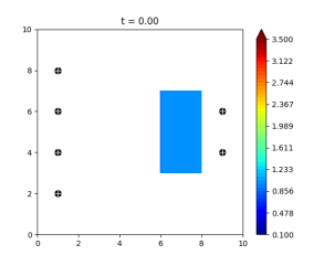
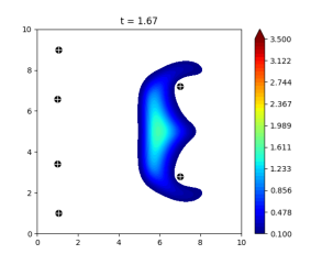
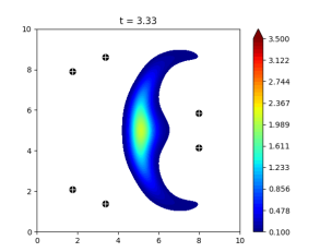
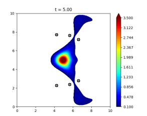
This integration is computed through a grid $3000\times 3000$. The resulting final cost, common to all players, is $10.54$.

3.4 Competition/Cooperation among Attractive/Repulsive Agents

Finally, the following integrations of (2.1) show first that cooperation arises also between attractive and repulsive agents. Then, it emphasizes the clear difference between cooperation and competition. Consider first the case

$$\begin{array}[]{@{}r@{\;}c@{\;}l@{}}N&=&2\,,\\ k&=&3\,,\\ m&=&6\,,\\ T&=&5\,,\end{array}\qquad\begin{array}[]{r@{\;}c@{\;}l@{}}a_{1}(\xi)=a_{3}(\xi)&=&-\frac{1}{\xi}\,e^{-\xi/5}\,,\\ a_{2}(\xi)&=&\frac{1}{\xi}\,e^{-\xi/5}\,,\\ v(t,x,P)&=&\mbox{as in~{}\eqref{eq:velocity-simulation}}\,,\\ U&=&1\,,\end{array}\qquad\begin{array}[]{r@{\;}c@{\;}l@{}}\bar{\rho}&=&\chi_{[1,2]\times[3,7]},\\ \bar{P}_{1}&=&(1,1),\\ \bar{P}_{2}&=&(1,5),\\ \bar{P}_{3}&=&(1,9),\end{array}\qquad\begin{array}[]{r@{\;}c@{\;}l@{}}\mathcal{T}_{1}&=&\left\{(9,5)\right\}.\end{array}$$ (3.6)

whose solution is depicted in Figure 4, first line.

Figure 4: Upper line, integration of (2.1) with parameters (3.6) and with the same cost for all players $\psi_{1}(x)=\psi_{2}(x)=\psi_{3}(x)=d(x,\mathcal{T}_{1})$. In the lower line, we set $\psi_{1}=\psi_{3}=-\psi_{2}$ as in (3.7). As a result, $P_{1}$ and $P_{3}$ steal most of the followers to $P_{2}$. In both cases, $P_{1}$ and $P_{3}$ are repulsive, while $P_{2}$ is attracting.

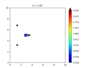
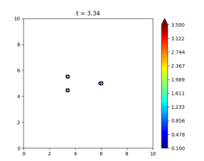
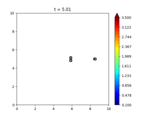
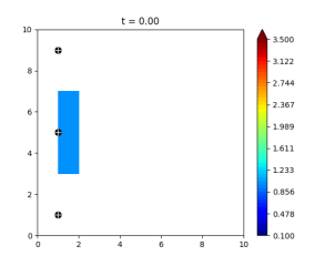
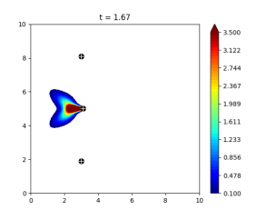
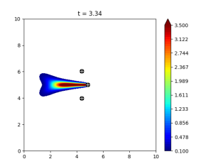
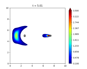
The final cost is $2.04$, the density $\rho$ being highly concentrated near to the target $\mathcal{T}_{1}$. Then, we keep the same parameters, but modify the costs of $P_{1}$ and $P_{3}$ setting

$$\psi_{1}(x)=\psi_{3}(x)=-d(x,\mathcal{T}_{1})\quad\mbox{ and }\quad\psi_{2}(x)=d(x,\mathcal{T}_{1})\,.$$ (3.7)

The resulting evolution is in Figure 4, second line. Note that $P_{1}$ and $P_{3}$ follow now a quite different trajectory, “cutting” the density $\rho$ so that the final cost of $P_{2}$ raises to $26.68$. In both integrations, the mesh consists of $3000\times 3000$ points.

4 Technical Details

Throughout, the continuous dependence of $V$ and $v$ on $t$ can be easily relaxed to mere measurability. In view of the applications below, the following result on ordinary differential equations deserves being recalled.

Lemma 4.1 ([2, Chapter 3]).

Let $V_{1},V_{2}\in\mathbf{C^{0}}([0,T]\times{\mathbb{R}}^{N};{\mathbb{R}}^{N})$ be such that the maps $x\to V_{i}(t,x)$ are in $\mathbf{C^{0,1}}({\mathbb{R}}^{N};{\mathbb{R}}^{N})$ for $i=1,2$ and for all $t\in[0,T]$. Then, for all $(\bar{t},\bar{x})\in[0,T]\times{\mathbb{R}}^{N}$ and $i\in\left\{1,2\right\}$, the Cauchy Problem

$$\left\{\begin{array}[]{l}\dot{x}=V_{i}(t,x)\\ x(\bar{t})=\bar{x}\end{array}\right.$$ (4.1)

admits, on the interval $[0,T]$, the unique solution $t\to X_{i}(t;\bar{t},\bar{x})$ and the following estimate holds, for all $t\in[0,T]$:

$$\begin{split}{\left\|X_{1}(t;\bar{t},\bar{x})-X_{2}(t;\bar{t},\bar{x})\right\|}\leq{}&{\left\|V_{1}-V_{2}\right\|}_{\mathbf{L^{1}}(\langle\bar{t},t\rangle;\mathbf{L^{\infty}}({\mathbb{R}}^{N};{\mathbb{R}}))}\\ &\times\exp\left({\left\|D_{x}V_{2}\right\|}_{\mathbf{L^{\infty}}(\langle\bar{t},t\rangle\times{\mathbb{R}}^{N};{\mathbb{R}}^{N\times N})}{\left|t-\bar{t}\right|}\right)\,.\end{split}$$ (4.2)

If moreover $x\to V_{i}(t,x)\in\mathbf{C^{1}}({\mathbb{R}}^{N};{\mathbb{R}}^{N})$ for all $t\in[0,T]$, the map $x\to X_{i}(t;\bar{t},\bar{x})$ is differentiable and its derivative $t\to D_{x}X_{i}(t;\bar{t},\bar{x})$ solves the linear matrix ordinary differential equation

$$\left\{\begin{array}[]{l}\dot{Y}=D_{x}V_{i}\left(t,X_{i}(t;\bar{t},\bar{x})\right)\,Y\\ Y(\bar{t})=\mathop{\mathbf{Id}}\,.\end{array}\right.$$ (4.3)

Lemma 4.2.

Let $V\in\mathbf{C^{0}}([0,T]\times{\mathbb{R}}^{N};{\mathbb{R}}^{N})$ be such that the map $x\to V(t,x)$ is in $\mathbf{C^{1}}({\mathbb{R}}^{N};{\mathbb{R}}^{N})$ for $i=1,2$ and for all $t\in[0,T]$. Then, for all $\bar{t}\in\left[0,T\right[$, $i\in\left\{1,2\right\}$, and $\bar{\rho}\in\mathbf{L^{1}}({\mathbb{R}}^{N};{\mathbb{R}})$, the Cauchy Problem

$$\left\{\begin{array}[]{l}\partial_{t}\rho+\mathinner{\mathop{\rm div}}_{x}\left(\rho\,V(t,x)\right)=0\\ \rho(\bar{t},x)=\bar{\rho}(x)\end{array}\right.$$ (4.4)

admits, on the interval $[\bar{t},T]$, the unique Kružkov solution

$$\rho(t,x)=\bar{\rho}\left(X(\bar{t};t,x)\right)\;\exp\left(-\int_{\bar{t}}^{t}\mathinner{\mathop{\rm div}}_{x}V\left(\tau,X(\tau;t,x)\right)\mathinner{\mathrm{d}{\tau}}\right)$$ (4.5)

and if $\mathop{\mathrm{missing}}{spt}\bar{\rho}$ is bounded, then

$$\mathop{\mathrm{missing}}{spt}\rho(t)\subseteq B\left(\mathop{\mathrm{missing}}{spt}\rho(\bar{t}),{\left\|V\right\|}_{\mathbf{L^{\infty}}(\langle\bar{t},t\rangle\times\mathop{\mathrm{missing}}{spt}\bar{\rho};{\mathbb{R}}^{N})}{\left|t-\bar{t}\right|}\,e^{{\left\|D_{x}V\right\|}_{\mathbf{L^{\infty}}(\langle\bar{t},t\rangle\times{\mathbb{R}}^{N};{\mathbb{R}}^{N\times N})}{\left|t-\bar{t}\right|}}\right).$$ (4.6)

Proof.

The fact that (4.5) solves (4.4) in Kružkov sense follows from [7, Lemma 5.1]. To prove (4.6), compute

$${\left\|X(t;\bar{t},x)-x\right\|} \leq {\left|\int_{\bar{t}}^{t}{\left\|V\left(\tau;X(\tau;\bar{t},x)\right)\right\|}\mathinner{\mathrm{d}{\tau}}\right|}$$

$$\leq {\left|\int_{\bar{t}}^{t}\left({\left\|V(\tau,x)\right\|}+{\left\|V\left(\tau;X(\tau;\bar{t},x)\right)-V(\tau,x)\right\|}\right)\mathinner{\mathrm{d}{\tau}}\right|}$$

$$\leq {\left\|V\right\|}_{\mathbf{L^{\infty}}(\langle\bar{t},t\rangle\times\mathop{\mathrm{missing}}{spt}\bar{\rho};{\mathbb{R}}^{N})}{\left|t-\bar{t}\right|}$$

$$\quad+{\left|\int_{\bar{t}}^{t}{\left\|D_{x}V\right\|}_{\mathbf{L^{\infty}}(\langle\bar{t},t\rangle\times{\mathbb{R}}^{N};{\mathbb{R}}^{N\times N})}{\left\|X(\tau;\bar{t},x)-x\right\|}\mathinner{\mathrm{d}{\tau}}\right|}$$

and by Grönwall Lemma, see, e.g., [2, Chapter 3, Lemma 3.1],

$${\left\|X(t;\bar{t},x)-x\right\|}\leq{\left\|V\right\|}_{\mathbf{L^{\infty}}(\langle\bar{t},t\rangle\times\mathop{\mathrm{missing}}{spt}\bar{\rho};{\mathbb{R}}^{N})}\,{\left|t-\bar{t}\right|}\;e^{{\left\|D_{x}V\right\|}_{\mathbf{L^{\infty}}(\langle\bar{t},t\rangle\times{\mathbb{R}}^{N};{\mathbb{R}}^{N\times N})}{\left|t-\bar{t}\right|}}\,,$$

completing the proof. ∎

Lemma 4.3.

Let $V_{1},V_{2}\in\mathbf{C^{0}}([0,T]\times{\mathbb{R}}^{N};{\mathbb{R}}^{N})$ be such that both maps $x\to V_{i}(t,x)$, $i=1,2$, are in $\mathbf{C^{1,1}}([0,T]\times{\mathbb{R}}^{N};{\mathbb{R}}^{N})$. If $\bar{\rho}\in\mathbf{C^{0,1}}({\mathbb{R}}^{N};{\mathbb{R}})$, then

$${\left\|\rho_{1}(t)-\rho_{2}(t)\right\|}_{\mathbf{L^{1}}({\mathbb{R}}^{N};{\mathbb{R}})}$$

$$\leq {\left\|\mathinner{\mathop{\rm grad}}_{x}\bar{\rho}\right\|}_{\mathbf{L^{\infty}}({\mathbb{R}}^{N};{\mathbb{R}}^{N})}\;\,\mathcal{L}^{N}\!\left(\mathop{\mathrm{missing}}{spt}\bar{\rho},Ce^{C{\left|t-\bar{t}\right|}}{\left|t-\bar{t}\right|}\right)e^{2C{\left|t-\bar{t}\right|}}{\left\|V_{1}-V_{2}\right\|}_{\mathbf{L^{1}}(\langle\bar{t},t\rangle;\mathbf{L^{\infty}}({\mathbb{R}}^{N};{\mathbb{R}}))}$$

$$\!\!+\left({\left\|\mathinner{\mathop{\rm div}}_{x}(V_{1}-V_{2})\right\|}_{\mathbf{L^{\infty}}(\langle\bar{t},t\rangle\times{\mathbb{R}}^{N};{\mathbb{R}})}+C{\left\|V_{1}-V_{2}\right\|}_{\mathbf{L^{1}}(\langle\bar{t},t\rangle;\mathbf{L^{\infty}}({\mathbb{R}}^{N};{\mathbb{R}}))}\right){\left\|\bar{\rho}\right\|}_{\mathbf{L^{1}}({\mathbb{R}}^{N};{\mathbb{R}})}e^{2C{\left|t-\bar{t}\right|}}{\left|t-\bar{t}\right|}$$

where

$$C=\max_{i=1,2}\left\{\begin{array}[]{l}{\left\|V_{i}\right\|}_{\mathbf{L^{\infty}}(\langle\bar{t},t\rangle\times{\mathbb{R}}^{N};{\mathbb{R}}^{N})}\\ {\left\|D_{x}V_{i}\right\|}_{\mathbf{L^{\infty}}(\langle\bar{t},t\rangle\times{\mathbb{R}}^{N};{\mathbb{R}}^{N\times N})}\\ {\left\|\mathinner{\mathop{\rm grad}}_{x}\mathinner{\mathop{\rm div}}_{x}V_{i}\right\|}_{\mathbf{L^{\infty}}(\langle\bar{t},t\rangle\times{\mathbb{R}}^{N};{\mathbb{R}}^{N})}\end{array}\right\}\,.$$ (4.7)

Proof.

Using (4.5) and the triangle inequality, we have

$${\left\|\rho_{1}(t)-\rho_{2}(t)\right\|}_{\mathbf{L^{1}}({\mathbb{R}}^{N};{\mathbb{R}})}\leq(I)+(II)+(III)$$

where

$$(I) = \int_{{\mathbb{R}}^{N}}{\left|\bar{\rho}\left(X_{1}(\bar{t};t,x)\right)-\bar{\rho}\left(X_{2}(\bar{t};t,x)\right)\right|}\exp{\left|\int_{\bar{t}}^{t}\mathinner{\mathop{\rm div}}_{x}V_{1}\left(\tau,X_{1}(\tau;t,x)\right)\mathinner{\mathrm{d}{\tau}}\right|}\mathinner{\mathrm{d}{x}}$$

$$(II) = \int_{{\mathbb{R}}^{N}}\bar{\rho}\left(X_{2}(\bar{t};t,x)\right)$$

$$\times \!\!\!{\left|\exp\left[-\int_{\bar{t}}^{t}\mathinner{\mathop{\rm div}}_{x}V_{1}\left(\tau,X_{1}(\tau;t,x)\right)\mathinner{\mathrm{d}{\tau}}\right]-\exp\left[-\int_{\bar{t}}^{t}\mathinner{\mathop{\rm div}}_{x}V_{2}\left(\tau,X_{1}(\tau;t,x)\right)\mathinner{\mathrm{d}{\tau}}\right]\right|}\mathinner{\mathrm{d}{x}}$$

$$(III) = \int_{{\mathbb{R}}^{N}}\bar{\rho}\left(X_{2}(\bar{t};t,x)\right)$$

$$\times \!\!\!{\left|\exp\left[-\int_{\bar{t}}^{t}\mathinner{\mathop{\rm div}}_{x}V_{2}\left(\tau,X_{1}(\tau;t,x)\right)\mathinner{\mathrm{d}{\tau}}\right]-\exp\left[-\int_{\bar{t}}^{t}\mathinner{\mathop{\rm div}}_{x}V_{2}\left(\tau,X_{2}(\tau;t,x)\right)\mathinner{\mathrm{d}{\tau}}\right]\right|}\mathinner{\mathrm{d}{x}}$$

and we now bound the three terms separately. To estimate $(I)$, observe that by (4.6)

$$\bigcup_{i=1}^{2}\mathop{\mathrm{missing}}{spt}\rho_{i}(t)\subseteq B\left(\mathop{\mathrm{missing}}{spt}\bar{\rho},\max_{i=1,2}{\left\|V_{i}\right\|}_{\mathbf{L^{\infty}}(\langle\bar{t},t\rangle\times\mathop{\mathrm{missing}}{spt}\bar{\rho};{\mathbb{R}}^{N})}\exp\left({\left\|D_{x}V_{i}\right\|}_{\mathbf{L^{\infty}}(\langle\bar{t},t\rangle\times{\mathbb{R}}^{N};{\mathbb{R}}^{N})}{\left|t-\bar{t}\right|}\right){\left|t-\bar{t}\right|}\right)$$

and, using (4.2),

$$(I) = \int_{\bigcup_{i=1}^{2}\mathop{\mathrm{missing}}{spt}\rho_{i}(t)}{\left|\bar{\rho}\left(X_{1}(\bar{t};t,x)\right)-\bar{\rho}\left(X_{2}(\bar{t};t,x)\right)\right|}\exp{\left|\int_{\bar{t}}^{t}\mathinner{\mathop{\rm div}}_{x}V_{1}\left(\tau,X_{1}(\tau;t,x)\right)\mathinner{\mathrm{d}{\tau}}\right|}\mathinner{\mathrm{d}{x}}$$

$$\leq \int_{\bigcup_{i=1}^{2}\mathop{\mathrm{missing}}{spt}\rho_{i}(t)}{\left\|\mathinner{\mathop{\rm grad}}_{x}\bar{\rho}\right\|}_{\mathbf{L^{\infty}}({\mathbb{R}}^{N};{\mathbb{R}}^{N})}{\left\|X_{1}(\bar{t};t,x)-X_{2}(\bar{t};t,x)\right\|}$$

$$\qquad\qquad\times\exp\left({\left\|D_{x}V_{1}\right\|}_{\mathbf{L^{\infty}}(\langle\bar{t},t\rangle\times{\mathbb{R}}^{N};{\mathbb{R}}^{N})}{\left|t-\bar{t}\right|}\right)\mathinner{\mathrm{d}{x}}$$

$$\leq {\left\|\mathinner{\mathop{\rm grad}}_{x}\bar{\rho}\right\|}_{\mathbf{L^{\infty}}({\mathbb{R}}^{N};{\mathbb{R}}^{N})}$$

$$\times\mathcal{L}^{N}\!\left(\mathop{\mathrm{missing}}{spt}\bar{\rho},\max_{i=1,2}{\left\|V_{i}\right\|}_{\mathbf{L^{\infty}}(\langle\bar{t},t\rangle\times\mathop{\mathrm{missing}}{spt}\bar{\rho};{\mathbb{R}}^{N})}\exp\left({\left\|D_{x}V_{i}\right\|}_{\mathbf{L^{\infty}}(\langle\bar{t},t\rangle\times{\mathbb{R}}^{N};{\mathbb{R}}^{N\times N})}{\left|t-\bar{t}\right|}\right){\left|t-\bar{t}\right|}\right)\;$$

$$\quad\times{\left\|V_{1}-V_{2}\right\|}_{\mathbf{L^{1}}(\langle\bar{t},t\rangle;\mathbf{L^{\infty}}({\mathbb{R}}^{N};{\mathbb{R}}))}$$

$$\quad\times\exp\left(\left({\left\|D_{x}V_{1}\right\|}_{\mathbf{L^{\infty}}((\langle\bar{t},t\rangle\times{\mathbb{R}}^{N};{\mathbb{R}}^{N\times N})}+{\left\|D_{x}V_{2}\right\|}_{\mathbf{L^{\infty}}((\langle\bar{t},t\rangle\times{\mathbb{R}}^{N};{\mathbb{R}}^{N\times N})}\right){\left|t-\bar{t}\right|}\right)\,.$$

Passing to the estimate of $(II)$, using the inequality ${\left|e^{a}-e^{b}\right|}\leq e^{\max\{a,b\}}{\left|a-b\right|}$,

$${\left|\exp\left(-\int_{\bar{t}}^{t}\mathinner{\mathop{\rm div}}_{x}V_{1}\left(\tau,X_{1}(\tau;t,x)\right)\mathinner{\mathrm{d}{\tau}}\right)-\exp\left(-\int_{\bar{t}}^{t}\mathinner{\mathop{\rm div}}_{x}V_{2}\left(\tau,X_{1}(\tau;t,x)\right)\mathinner{\mathrm{d}{\tau}}\right)\right|}$$

$$\leq \exp\left(\max_{i=1,2}{\left\|D_{x}V_{i}\right\|}_{\mathbf{L^{\infty}}(\langle\bar{t},t\rangle\times{\mathbb{R}}^{N};{\mathbb{R}}^{N\times N})}\,{\left|t-\bar{t}\right|}\right)$$

$$\quad\times{\left|\int_{\bar{t}}^{t}{\left|\mathinner{\mathop{\rm div}}_{x}V_{2}\left(\tau,X_{1}(\tau;t,x)\right)-\mathinner{\mathop{\rm div}}_{x}V_{1}\left(\tau,X_{1}(\tau;t,x)\right)\right|}\mathinner{\mathrm{d}{\tau}}\right|}$$

$$\leq \exp\left(\max_{i=1,2}{\left\|D_{x}V_{i}\right\|}_{\mathbf{L^{\infty}}(\langle\bar{t},t\rangle\times{\mathbb{R}}^{N};{\mathbb{R}}^{N\times N})}\,{\left|t-\bar{t}\right|}\right)\;{\left\|\mathinner{\mathop{\rm div}}_{x}V_{1}-\mathinner{\mathop{\rm div}}_{x}V_{2}\right\|}_{\mathbf{L^{\infty}}(\langle\bar{t},t\rangle\times{\mathbb{R}}^{N};{\mathbb{R}})}\;{\left|t-\bar{t}\right|}$$

so that

$$(II) \leq \exp\left(\max_{i=1,2}{\left\|D_{x}V_{i}\right\|}_{\mathbf{L^{\infty}}(\langle\bar{t},t\rangle\times{\mathbb{R}}^{N};{\mathbb{R}}^{N\times N})}\,{\left|t-\bar{t}\right|}\right)\;{\left\|\mathinner{\mathop{\rm div}}_{x}(V_{1}-V_{2})\right\|}_{\mathbf{L^{\infty}}(\langle\bar{t},t\rangle\times{\mathbb{R}}^{N};{\mathbb{R}})}$$

$$\quad\times{\left\|\bar{\rho}\right\|}_{\mathbf{L^{1}}({\mathbb{R}}^{N};{\mathbb{R}})}\;{\left|t-\bar{t}\right|}\,.$$

To bound $(III)$, use (4.2) and proceed similarly:

$${\left|\exp\left(-\int_{\bar{t}}^{t}\mathinner{\mathop{\rm div}}_{x}V_{2}\left(\tau,X_{1}(\tau;t,x)\right)\mathinner{\mathrm{d}{\tau}}\right)-\exp\left(-\int_{\bar{t}}^{t}\mathinner{\mathop{\rm div}}_{x}V_{2}\left(\tau,X_{2}(\tau;t,x)\right)\mathinner{\mathrm{d}{\tau}}\right)\right|}$$

$$\leq \exp\left({\left\|D_{x}V_{2}\right\|}_{\mathbf{L^{\infty}}(\langle\bar{t},t\rangle\times{\mathbb{R}}^{N};{\mathbb{R}}^{N\times N})}{\left|t-\bar{t}\right|}\right)$$

$$\quad\times{\left|\int_{\bar{t}}^{t}{\left|\mathinner{\mathop{\rm div}}_{x}V_{2}\left(\tau,X_{1}(\tau;t,x)\right)-\mathinner{\mathop{\rm div}}_{x}V_{2}\left(\tau,X_{2}(\tau;t,x)\right)\right|}\mathinner{\mathrm{d}{\tau}}\right|}$$

$$\leq \exp\left(2{\left\|D_{x}V_{2}\right\|}_{\mathbf{L^{\infty}}(\langle\bar{t},t\rangle\times{\mathbb{R}}^{N};{\mathbb{R}}^{N\times N})}{\left|t-\bar{t}\right|}\right)\;{\left\|\mathinner{\mathop{\rm grad}}_{x}\mathinner{\mathop{\rm div}}_{x}V_{2}\right\|}_{\mathbf{L^{\infty}}(\langle\bar{t},t\rangle\times{\mathbb{R}}^{N};{\mathbb{R}}^{N})}$$

$$\qquad\times{\left\|V_{1}-V_{2}\right\|}_{\mathbf{L^{1}}(\langle\bar{t},t\rangle;\mathbf{L^{\infty}}({\mathbb{R}}^{N};{\mathbb{R}}))}\;{\left|t-\bar{t}\right|}$$

so that

$$(III) \leq \exp\left(2{\left\|D_{x}V_{2}\right\|}_{\mathbf{L^{\infty}}(\langle\bar{t},t\rangle\times{\mathbb{R}}^{N};{\mathbb{R}}^{N\times N})}{\left|t-\bar{t}\right|}\right){\left\|\bar{\rho}\right\|}_{\mathbf{L^{1}}({\mathbb{R}}^{N};{\mathbb{R}})}\;{\left\|\mathinner{\mathop{\rm grad}}_{x}\mathinner{\mathop{\rm div}}_{x}V_{2}\right\|}_{\mathbf{L^{\infty}}(\langle\bar{t},t\rangle\times{\mathbb{R}}^{N};{\mathbb{R}}^{N})}$$

$$\qquad\times{\left\|V_{1}-V_{2}\right\|}_{\mathbf{L^{1}}(\langle\bar{t},t\rangle;\mathbf{L^{\infty}}({\mathbb{R}}^{N};{\mathbb{R}}))}\;{\left|t-\bar{t}\right|}$$

Summing up the expressions obtained:

$${\left\|\rho_{1}(t)-\rho_{2}(t)\right\|}_{\mathbf{L^{1}}({\mathbb{R}}^{N};{\mathbb{R}})}$$

$$\leq {\left\|\mathinner{\mathop{\rm grad}}_{x}\bar{\rho}\right\|}_{\mathbf{L^{\infty}}({\mathbb{R}}^{N};{\mathbb{R}}^{N})}\;{\left\|V_{1}-V_{2}\right\|}_{\mathbf{L^{1}}(\langle\bar{t},t\rangle;\mathbf{L^{\infty}}({\mathbb{R}}^{N};{\mathbb{R}}))}$$

$$\quad\times\mathcal{L}^{N}\left(\mathop{\mathrm{missing}}{spt}\bar{\rho},\max_{i=1,2}{\left\|V_{i}\right\|}_{\mathbf{L^{\infty}}(\langle\bar{t},t\rangle\times\mathop{\mathrm{missing}}{spt}\bar{\rho})}\exp\left({\left\|D_{x}V_{i}\right\|}_{\mathbf{L^{\infty}}(\langle\bar{t},t\rangle\times{\mathbb{R}}^{N})}{\left|t-\bar{t}\right|}\right){\left|t-\bar{t}\right|}\right)$$

$$\quad\times\exp\left(\left({\left\|D_{x}V_{1}\right\|}_{\mathbf{L^{\infty}}((\langle\bar{t},t\rangle\times{\mathbb{R}}^{N};{\mathbb{R}}^{N\times N})}+{\left\|D_{x}V_{2}\right\|}_{\mathbf{L^{\infty}}((\langle\bar{t},t\rangle\times{\mathbb{R}}^{N};{\mathbb{R}}^{N\times N})}\right){\left|t-\bar{t}\right|}\right)$$

$$+\exp\left[\max_{i=1,2}{\left\|D_{x}V_{i}\right\|}_{\mathbf{L^{\infty}}(\langle\bar{t},t\rangle\times{\mathbb{R}}^{N})}{\left|t-\bar{t}\right|}\right]{\left\|\mathinner{\mathop{\rm div}}_{x}(V_{1}-V_{2})\right\|}_{\mathbf{L^{\infty}}(\langle\bar{t},t\rangle\times{\mathbb{R}}^{N};{\mathbb{R}})}{\left\|\bar{\rho}\right\|}_{\mathbf{L^{1}}({\mathbb{R}}^{N};{\mathbb{R}})}{\left|t-\bar{t}\right|}$$

$$+\exp\left(2{\left\|D_{x}V_{2}\right\|}_{\mathbf{L^{\infty}}(\langle\bar{t},t\rangle\times{\mathbb{R}}^{N};{\mathbb{R}}^{N\times N})}{\left|t-\bar{t}\right|}\right)\;{\left\|\bar{\rho}\right\|}_{\mathbf{L^{1}}({\mathbb{R}}^{N};{\mathbb{R}})}\;{\left\|\mathinner{\mathop{\rm grad}}_{x}\mathinner{\mathop{\rm div}}_{x}V_{2}\right\|}_{\mathbf{L^{\infty}}(\langle\bar{t},t\rangle\times{\mathbb{R}}^{N};{\mathbb{R}}^{N})}$$

$$\qquad\times{\left\|V_{1}-V_{2}\right\|}_{\mathbf{L^{1}}(\langle\bar{t},t\rangle;\mathbf{L^{\infty}}({\mathbb{R}}^{N};{\mathbb{R}}))}\;{\left|t-\bar{t}\right|}$$

Introduce $C$ as in (4.7). Then,

$${\left\|\rho_{1}(t)-\rho_{2}(t)\right\|}_{\mathbf{L^{1}}({\mathbb{R}}^{N};{\mathbb{R}})}$$

$$\leq {\left\|\mathinner{\mathop{\rm grad}}_{x}\bar{\rho}\right\|}_{\mathbf{L^{\infty}}({\mathbb{R}}^{N};{\mathbb{R}}^{N})}\;\mathcal{L}^{N}\left(\mathop{\mathrm{missing}}{spt}\bar{\rho},Ce^{C{\left|t-\bar{t}\right|}}{\left|t-\bar{t}\right|}\right)e^{2C{\left|t-\bar{t}\right|}}{\left\|V_{1}-V_{2}\right\|}_{\mathbf{L^{1}}(\langle\bar{t},t\rangle;\mathbf{L^{\infty}}({\mathbb{R}}^{N};{\mathbb{R}}))}$$

$$+{\left\|\bar{\rho}\right\|}_{\mathbf{L^{1}}({\mathbb{R}}^{N};{\mathbb{R}})}\;e^{2C{\left|t-\bar{t}\right|}}\;{\left\|\mathinner{\mathop{\rm div}}_{x}(V_{1}-V_{2})\right\|}_{\mathbf{L^{\infty}}(\langle\bar{t},t\rangle\times{\mathbb{R}}^{N};{\mathbb{R}})}\;{\left|t-\bar{t}\right|}$$

$$+{\left\|\bar{\rho}\right\|}_{\mathbf{L^{1}}({\mathbb{R}}^{N};{\mathbb{R}})}\;C\;e^{2C{\left|t-\bar{t}\right|}}\;{\left\|V_{1}-V_{2}\right\|}_{\mathbf{L^{1}}(\langle\bar{t},t\rangle;\mathbf{L^{\infty}}({\mathbb{R}}^{N};{\mathbb{R}}))}\;{\left|t-\bar{t}\right|}$$

completing the proof. ∎

Proof of Proposition 2.1.  The first statement follows from Lemma 4.2. Define $V_{i}(t,x)=v\left(t,x,P_{i}(t)\right)$, with $P_{i}(t)=\bar{P}+\int_{0}^{t}u_{i}(\tau)\mathinner{\mathrm{d}{\tau}}$, for $i=1,2$. Then, direct computations yield:

$${\left\|V_{i}\right\|}_{\mathbf{L^{\infty}}([0,t]\times{\mathbb{R}}^{N};{\mathbb{R}}^{N})} \leq {\left\|v\right\|}_{\mathbf{L^{\infty}}([0,t]\times{\mathbb{R}}^{N}\times{\mathbb{R}}^{m};{\mathbb{R}}^{N})}\,.$$

$${\left\|D_{x}V_{i}\right\|}_{\mathbf{L^{\infty}}([0,t]\times{\mathbb{R}}^{N};{\mathbb{R}}^{N\times N})} = {\left\|D_{x}v\right\|}_{\mathbf{L^{\infty}}([0,t]\times{\mathbb{R}}^{N}\times{\mathbb{R}}^{m};{\mathbb{R}}^{N\times N)}}\,.$$

$${\left\|\mathinner{\mathop{\rm grad}}_{x}\mathinner{\mathop{\rm div}}_{x}V_{i}\right\|}_{\mathbf{L^{\infty}}([0,t]\times{\mathbb{R}}^{N};{\mathbb{R}}^{N})} \leq {\left\|\mathinner{\mathop{\rm grad}}_{x}\mathinner{\mathop{\rm div}}_{x}v\right\|}_{\mathbf{L^{\infty}}([0,t]\times{\mathbb{R}}^{N}\times{\mathbb{R}}^{m};{\mathbb{R}}^{N})}\,.$$

$${\left\|V_{1}-V_{2}\right\|}_{\mathbf{L^{1}}([0,t];\mathbf{L^{\infty}}({\mathbb{R}}^{N};{\mathbb{R}}))} = \int_{0}^{t}\sup_{x\in{\mathbb{R}}^{N}}{\left\|v\left(\tau,x,P_{1}(\tau)\right)-v\left(\tau,x,P_{2}(\tau)\right)\right\|}\mathinner{\mathrm{d}{\tau}}$$

$$\leq {\left\|D_{P}v\right\|}_{\mathbf{L^{\infty}}([0,t]\times{\mathbb{R}}^{N}\times{\mathbb{R}}^{m};{\mathbb{R}}^{N\times m})}\,t\,{\left\|P_{1}-P_{2}\right\|}_{\mathbf{L^{\infty}}([0,t];{\mathbb{R}}^{m})}\,.$$

$${\left\|\mathinner{\mathop{\rm div}}_{x}(V_{1}-V_{2})\right\|}_{\mathbf{L^{\infty}}([0,t]\times{\mathbb{R}}^{N};{\mathbb{R}})} \leq {\left\|\mathinner{\mathop{\rm div}}_{x}v\right\|}_{\mathbf{L^{\infty}}([0,t]\times{\mathbb{R}}^{N}\times{\mathbb{R}}^{m};{\mathbb{R}})}\,{\left\|P_{1}-P_{2}\right\|}_{\mathbf{L^{\infty}}([0,t];{\mathbb{R}}^{N})}\,.$$

Now, (2.2) directly follows from (4.2) in Lemma 4.1. To prove (2.1) use Lemma 4.3.   $\square$

We recall here, without proof, the following result about Gâteaux and Fréchet differentiability for later use.

Lemma 4.4 ([17, Lemma 1.15]).

Let $X,Y$ be Banach spaces, $A\subseteq X$ be open, $x_{o}\in A$ and $J\colon A\to Y$ be a map. Assume

1. $J$ is Gâteaux differentiable at all $x\in A$ in all directions $v\in X$;

2. the map $v\to D_{v}J(x)$ is linear and continuous for all $x\in A$;

3. $\lim\limits_{x\to x_{o}}\sup\limits_{{\left\|v\right\|}_{X}=1}{\left\|D_{v}J(x)-D_{v}J(x_{o})\right\|}_{Y}=0$.

Then, $J$ is Fréchet differentiable at $x_{o}$.

The next result describes the Fréchet differentiability of the characteristic curves.

Lemma 4.5.

Fix $t\in\left[0,T\right[$, $\Delta t\in\left]0,T-t\right]$ and $x\in{\mathbb{R}}^{N}$. If $v\in\mathbf{C^{2}}([0,T]\times{\mathbb{R}}^{N}\times{\mathbb{R}}^{N};{\mathbb{R}}^{N})$, then the map

$$\begin{array}[b]{ccccc}\mathcal{X}_{t,x}&\colon&{\mathbb{R}}^{N}&\to&\mathbf{C^{0}}([t,t+\Delta t];{\mathbb{R}}^{N})\\ &&w&\to&\mathcal{X}_{t,x}(w)\,,\end{array}$$

defined so that $\tau\to\left(\mathcal{X}_{t,x}(w)\right)\!(\tau)$ solves the Cauchy problem

$$\left\{\begin{array}[]{@{}l@{\,}}\xi^{\prime}=v\left(t,\xi,P(t)+(\tau-t)w\right)\\ \xi(t)=x\,,\end{array}\right.$$ (4.8)

is Fréchet differentiable in ${\mathbb{R}}^{N}$. Moreover $\mathcal{X}_{t,x}$ has the Taylor expansion

$$\mathcal{X}_{t,x}(w+\delta_{w})=\mathcal{X}_{t,x}(w)+D\mathcal{X}_{t,x}(w)\,\delta_{w}+o(\delta_{w})\quad\mbox{in }\mathbf{C^{0}}\mbox{ as }\delta_{w}\to 0$$

where $\tau\to\left(D\mathcal{X}_{t,x}(w)\right)(\tau)$ solves the linear first order $N\times N$ matrix differential equation

$$\left\{\begin{array}[]{l}Y^{\prime}=D_{x}v\left(t,\mathcal{X}_{t,x}(w)(\tau),P(t)+(\tau-t)w\right)Y\vspace{.2cm}\\ \qquad\qquad+(\tau-t)\,D_{P}v\left(t,\mathcal{X}_{t,x}(w)(\tau),P(t)+(\tau-t)w\right)\vspace{.2cm}\\ Y(t)=0\end{array}\right.$$ (4.9)

and the term $D\mathcal{X}_{t,x}(w)$ satisfies the expansion, as $\tau\to t$,

$$\left(D\mathcal{X}_{t,x}(w)\right)(\tau)=\dfrac{(\tau-t)^{2}}{2}\,D_{P}v\left(t,x,P(t)\right)+o(\tau-t)^{2}\,.$$ (4.10)

Proof.

Since $t$ and $x$ are kept fixed throughout this proof, we write $\mathcal{X}(w)$ for $\mathcal{X}_{t,x}(w)$. Recall that, for $\tau\in[t,t+\Delta t]$,

$$\mathcal{X}(w)(\tau)=x+\int_{t}^{\tau}v\left(t,\mathcal{X}(w)(s),P(t)+(s-t)w\right)\mathinner{\mathrm{d}{s}}\,.$$

Fix a direction $\delta_{w}\in{\mathbb{R}}^{N}\setminus\{0\}$. First we show the boundedness of the difference quotient

$$\frac{{\left\|\mathcal{X}(w+\varepsilon\delta_{w})(\tau)-\mathcal{X}(w)(\tau)\right\|}}{\varepsilon}.$$

For $\tau\in[t,t+\Delta t]$, we have

$$\frac{1}{\varepsilon}{\left\|\mathcal{X}(w+\varepsilon\delta_{w})(\tau)-\mathcal{X}(w)(\tau)\right\|}$$

$$\leq \frac{1}{\varepsilon}\int_{t}^{\tau}{\left\|v\left(t,\mathcal{X}(w+\varepsilon\delta_{w})(s),P(t)+(s-t)(w+\varepsilon\delta_{w})\right){-}v\left(t,\mathcal{X}(w)(s),P(t)+(s-t)w\right)\right\|}\!\mathinner{\mathrm{d}{s}}$$

$$\leq \frac{1}{\varepsilon}\int_{t}^{\tau}\bigl{\|}v\left(t,\mathcal{X}(w+\varepsilon\delta_{w})(s),\!P(t)\!+\!(s-t)(w+\varepsilon\delta_{w})\right)\!-\!v\left(t,\mathcal{X}(w)(s),\!P(t)\!+\!(s-t)(w+\varepsilon\delta_{w})\right)\bigr{\|}\!\mathinner{\mathrm{d}{s}}$$

$$+\frac{1}{\varepsilon}\int_{t}^{\tau}{\left\|v\left(t,\mathcal{X}(w)(s),P(t)+(s-t)(w+\varepsilon\delta_{w})\right)-v\left(t,\mathcal{X}(w)(s),P(t)+(s-t)w\right)\right\|}\mathinner{\mathrm{d}{s}}$$

$$\leq {\left\|v\right\|}_{\mathbf{C^{1}}\left([0,T]\times{\mathbb{R}}^{N}\times{\mathbb{R}}^{N};{\mathbb{R}}^{N}\right)}\left[\int_{t}^{\tau}\frac{{\left\|\mathcal{X}(w+\varepsilon\delta_{w})(s)-\mathcal{X}(w)(s)\right\|}}{\varepsilon}\mathinner{\mathrm{d}{s}}+\int_{t}^{\tau}(s-t){\left\|\delta_{w}\right\|}\mathinner{\mathrm{d}{s}}\right]$$

$$\leq {\left\|v\right\|}_{\mathbf{C^{1}}\left([0,T]\times{\mathbb{R}}^{N}\times{\mathbb{R}}^{N};{\mathbb{R}}^{N}\right)}\left[\int_{t}^{\tau}\frac{{\left\|\mathcal{X}(w+\varepsilon\delta_{w})(s)-\mathcal{X}(w)(s)\right\|}}{\varepsilon}\mathinner{\mathrm{d}{s}}+\left(\Delta t\right)^{2}{\left\|\delta_{w}\right\|}\right].$$

Hence an application of Grönwall Lemma, see, e.g., [2, Chapter 3, Lemma 3.1] ensures that

$$\frac{{\left\|\mathcal{X}(w+\varepsilon\delta_{w})(\tau)-\mathcal{X}(w)(\tau)\right\|}}{\varepsilon}\leq K_{1}\left(\Delta t\right)^{3}{\left\|\delta_{w}\right\|}\exp\left(K_{1}\Delta t\right),$$ (4.11)

where $K_{1}={\left\|v\right\|}_{\mathbf{C^{1}}\left([0,T]\times{\mathbb{R}}^{N}\times{\mathbb{R}}^{N};{\mathbb{R}}^{N}\right)}$. Consequently

$$\lim_{\varepsilon\to 0}\sup_{\tau\in[t,t+\Delta t]}{\left\|\mathcal{X}(w+\varepsilon\delta_{w})(\tau)-\mathcal{X}(w)(\tau)\right\|}=0\,.$$ (4.12)

We now prove the existence of directional derivatives of $\mathcal{X}$ along the direction $\delta_{w}\in{\mathbb{R}}^{N}\setminus\{0\}$. Calling $\tau\to Y(\tau)$ the solution to the Cauchy problem (4.9), we have

$$\dfrac{\mathcal{X}(w+\varepsilon\delta_{w})(\tau)-\mathcal{X}(w)(\tau)}{\varepsilon}-Y(\tau)\;\delta_{w}$$

$$= \!\dfrac{1}{\varepsilon}\!\int_{t}^{\tau}\!\!\left[v\!\left(t,\mathcal{X}(w+\varepsilon\delta_{w})(s),P(t)+(s-t)(w+\varepsilon\delta_{w})\right)-v\!\left(t,\mathcal{X}(w)(s),P(t)+(s-t)w\right)\!\right]\!\mathinner{\mathrm{d}{s}}$$

$$-\int_{t}^{\tau}D_{x}v\left(t,\mathcal{X}(w)(s),P(t)+(s-t)w\right)Y(s)\mathinner{\mathrm{d}{s}}\,\delta_{w}$$

$$-\int_{t}^{\tau}(s-t)D_{P}v\left(t,\mathcal{X}(w)(s),P(t)+(s-t)w\right)\mathinner{\mathrm{d}{s}}\;\delta_{w}$$

$$= \dfrac{1}{\varepsilon}\int_{t}^{\tau}\bigl{[}v\!\left(t,\mathcal{X}(w+\varepsilon\delta_{w})(s),P(t)+(s-t)(w+\varepsilon\delta_{w})\right)$$

$$\qquad\qquad\qquad-v\!\left(t,\mathcal{X}(w)(s),P(t)+(s-t)(w+\delta_{w})\right)\bigr{]}\mathinner{\mathrm{d}{s}}$$

$$-\int_{t}^{\tau}D_{x}v\left(t,\mathcal{X}(w)(s),P(t)+(s-t)w\right)Y(s)\mathinner{\mathrm{d}{s}}\,\delta_{w}$$

$$+\dfrac{1}{\varepsilon}\int_{t}^{\tau}\!\!\left[v\!\left(t,\mathcal{X}(w)(s),P(t)+(s-t)(w+\varepsilon\delta_{w})\right)-v\!\left(t,\mathcal{X}(w)(s),P(t)+(s-t)w\right)\!\right]\!\mathinner{\mathrm{d}{s}}$$

$$-\int_{t}^{\tau}(s-t)D_{P}v\left(t,\mathcal{X}(w)(s),P(t)+(s-t)w\right)\mathinner{\mathrm{d}{s}}\;\delta_{w}$$

$$= \int_{t}^{\tau}\int_{0}^{1}\Bigl{(}D_{x}v\left(t,\vartheta\mathcal{X}(w+\varepsilon\delta_{w})(s)+(1-\vartheta)\mathcal{X}(w)(s),P(t)+(s-t)(w+\varepsilon\delta_{w})\right)\mathinner{\mathrm{d}{\vartheta}}$$

$$\qquad\qquad\qquad\times\dfrac{\mathcal{X}(w+\varepsilon\delta_{w})(s)-\mathcal{X}(w)(s)}{\varepsilon}\Bigr{)}\mathinner{\mathrm{d}{s}}$$

$$-\int_{t}^{\tau}D_{x}v\left(t,\mathcal{X}(w)(s),P(t)+(s-t)w\right)Y(s)\mathinner{\mathrm{d}{s}}\,\delta_{w}$$

$$+\int_{t}^{\tau}(s-t)\Bigl{(}\int_{0}^{1}D_{P}v\left(t,\mathcal{X}(w)(s),P(t)+(s-t)(w+(1-\vartheta)\varepsilon\delta_{w})\right)\mathinner{\mathrm{d}{\vartheta}}$$

$$\qquad\qquad\qquad\qquad-D_{P}v\left(t,\mathcal{X}(w)(s),P(t)+(s-t)w\right)\Bigr{)}\mathinner{\mathrm{d}{s}}\;\delta_{w}$$

$$= \int_{t}^{\tau}\int_{0}^{1}\Bigl{(}D_{x}v\left(t,\vartheta\mathcal{X}(w+\varepsilon\delta_{w})(s)+(1-\vartheta)\mathcal{X}(w)(s),P(t)+(s-t)(w+\varepsilon\delta_{w})\right)\mathinner{\mathrm{d}{\vartheta}}$$

$$\qquad\qquad\qquad\times\dfrac{\mathcal{X}(w+\varepsilon\delta_{w})(s)-\mathcal{X}(w)(s)}{\varepsilon}\Bigr{)}\mathinner{\mathrm{d}{s}}$$

$$\mp\int_{t}^{\tau}D_{x}v\left(t,\mathcal{X}(w)(s),P(t)+(s-t)w\right)\dfrac{\mathcal{X}(w+\varepsilon\delta_{w})(s)-\mathcal{X}(w)(s)}{\varepsilon}\mathinner{\mathrm{d}{s}}$$

$$-\int_{t}^{\tau}D_{x}v\left(t,\mathcal{X}(w)(s),P(t)+(s-t)w\right)Y(s)\mathinner{\mathrm{d}{s}}\,\delta_{w}$$

$$+\int_{t}^{\tau}(s-t)\Bigl{(}\int_{0}^{1}D_{P}v\left(t,\mathcal{X}(w)(s),P(t)+(s-t)(w+(1-\vartheta)\varepsilon\delta_{w})\right)\mathinner{\mathrm{d}{\vartheta}}$$

$$\qquad\qquad\qquad\qquad-D_{P}v\left(t,\mathcal{X}(w)(s),P(t)+(s-t)w\right)\Bigr{)}\mathinner{\mathrm{d}{s}}\;\delta_{w}$$

$$= \int_{t}^{\tau}\int_{0}^{1}\Bigl{(}D_{x}v\left(t,\vartheta\mathcal{X}(w+\varepsilon\delta_{w})(s)+(1-\vartheta)\mathcal{X}(w)(s),P(t)+(s-t)(w+\varepsilon\delta_{w})\right)\mathinner{\mathrm{d}{\vartheta}}$$

$$\qquad\qquad\qquad-D_{x}v\left(t,\mathcal{X}(w)(s),P(t)+(s-t)w\right)\Bigr{)}\frac{\mathcal{X}(w+\varepsilon\delta_{w})(s)-\mathcal{X}(w)(s)}{\varepsilon}\mathinner{\mathrm{d}{s}}$$

$$+\int_{t}^{\tau}D_{x}v\left(t,\mathcal{X}(w)(s),P(t)+(s-t)w\right)$$

$$\qquad\qquad\qquad\times\left(\dfrac{\mathcal{X}(w+\varepsilon\delta_{w})(s)-\mathcal{X}(w)(s)}{\varepsilon}-Y(s)\delta_{w}\right)\mathinner{\mathrm{d}{s}}$$

$$+\int_{t}^{\tau}(s-t)\Bigl{(}\int_{0}^{1}D_{P}v\left(t,\mathcal{X}(w)(s),P(t)+(s-t)(w+(1-\vartheta)\varepsilon\delta_{w})\right)\mathinner{\mathrm{d}{\vartheta}}$$

$$\qquad\qquad\qquad\qquad-D_{P}v\left(t,\mathcal{X}(w)(s),P(t)+(s-t)w\right)\Bigr{)}\mathinner{\mathrm{d}{s}}\;\delta_{w}$$

Calling $\mathinner{\mathcal{O}(1)}$ a constant dependent on the $\mathbf{C^{2}}$ norm of $v$ and on the right hand side of (4.11), the above equality leads to

$${\left\|\dfrac{\mathcal{X}(w+\varepsilon\delta_{w})(\tau)-\mathcal{X}(w)(\tau)}{\varepsilon}-Y(\tau)\;\delta_{w}\right\|}$$

$$\leq \mathinner{\mathcal{O}(1)}+\int_{t}^{\tau}\mathinner{\mathcal{O}(1)}\,{\left\|\dfrac{\mathcal{X}(w+\varepsilon\delta_{w})(\tau)-\mathcal{X}(w)(\tau)}{\varepsilon}-Y(\tau)\;\delta_{w}\right\|}\mathinner{\mathrm{d}{s}}$$

$$+\int_{t}^{\tau}\mathinner{\mathcal{O}(1)}\,(s-t)\,\varepsilon\mathinner{\mathrm{d}{s}}\,\delta_{w}\,.$$

Thanks to (4.12), an application of Grönwall Lemma proves the directional differentiability of $w\to\mathcal{X}(w)$ in the direction $\delta_{w}$.

To prove the differentiability of $\mathcal{X}$, we are left to verify that 2. and 3. in Lemma 4.4 hold. The linearity of $\delta_{w}\to D\mathcal{X}(w)(\delta_{w})$ is immediate, thanks to the homogeneous initial datum in (4.9). The assumed $\mathbf{C^{2}}$ regularity of $v$ ensures the $\mathbf{C^{1}}$ regularity of the right hand side in (4.9) and, hence, the boundedness of $\delta_{w}\to D\mathcal{X}(w)(\delta_{w})$ (in the sense of linear operators), completing the proof of 2. Standard theorems on the continuous dependence of solutions to ordinary differential equations from parameters, see, e.g., [2, Theorem 4.2], ensure that also 3. in Lemma 4.4 holds, completing the proof of the differentiability of $\mathcal{X}$.

The proof of the Taylor expansion (4.10) follows easily using (4.9). Indeed, by (4.9), we deduce that $Y(t)=Y^{\prime}(t)=0$, while $Y^{\prime\prime}(t)=D_{P}v\left(t,x,P(t)\right)$, so that, if $\tau\in[t,t+\Delta t]$, then

$$Y(\tau)=\frac{\left(\tau-t\right)^{2}}{2}D_{P}v\left(t,x,P(t)\right)+o\left(\left(\tau-t\right)^{2}\right).$$

This completes the proof of (4.10) and of the lemma. ∎

Proof of Lemma 2.3.  The first statement is a direct consequence of Lemma 4.2. To prove (2.9), we apply Lemma 4.3 with $V(\tau,x)=v(t,x,P(t)+(\tau-t)\,w)$ for $\tau\in[t,t+\Delta t]$:

$${\left\|V_{i}\right\|}_{\mathbf{L^{\infty}}([t,t+\Delta t]\times{\mathbb{R}}^{N};{\mathbb{R}}^{N})} \leq {\left\|v\right\|}_{\mathbf{L^{\infty}}([t,t+\Delta t]\times{\mathbb{R}}^{N}\times B(P(t),\Delta t{\left\|w_{i}\right\|});{\mathbb{R}}^{N})}\,,$$

$${\left\|D_{x}V_{i}\right\|}_{\mathbf{L^{\infty}}([t,t+\Delta t]\times{\mathbb{R}}^{N};{\mathbb{R}}^{N\times N})} \leq {\left\|D_{x}v\right\|}_{\mathbf{L^{\infty}}([t,t+\Delta t]\times{\mathbb{R}}^{N}\times B(P(t),\Delta t{\left\|w_{i}\right\|}),{\mathbb{R}}^{N\times N})}\,,$$

$${\left\|V_{1}-V_{2}\right\|}_{\mathbf{L^{1}}([t.t+\Delta t],\mathbf{L^{\infty}}({\mathbb{R}}^{N};{\mathbb{R}}^{N}))} \leq \frac{1}{2}\;{\left\|D_{P}v\right\|}_{\mathbf{L^{\infty}}([t,t+\Delta t]\times{\mathbb{R}}^{N}\times{\mathbb{R}}^{N};{\mathbb{R}}^{N\times N})}(\Delta t)^{2}{\left\|w_{1}-w_{2}\right\|}\,,$$

$${\left\|\mathinner{\mathop{\rm div}}_{x}(V_{1}-V_{2})\right\|}_{\mathbf{L^{\infty}}([t.t+\Delta t]\times{\mathbb{R}}^{N};{\mathbb{R}}^{N})} \leq {\left\|D_{P}\mathinner{\mathop{\rm div}}_{x}v\right\|}_{\mathbf{L^{\infty}}([t,t+\Delta t]\times{\mathbb{R}}^{N}\times{\mathbb{R}}^{N};{\mathbb{R}}^{N})}(\Delta t)\,{\left\|w_{1}-w_{2}\right\|}\,.$$

With the notation (2.10), and assuming that $C\geq 1$,

$${\left\|\rho_{1}(t+\Delta t)-\rho_{2}(t+\Delta t)\right\|}_{\mathbf{L^{1}}({\mathbb{R}}^{N};{\mathbb{R}})}$$

$$\leq {\left\|\mathinner{\mathop{\rm grad}}_{x}\bar{\rho}\right\|}_{\mathbf{L^{\infty}}({\mathbb{R}}^{N};{\mathbb{R}}^{N})}\;\mathcal{L}^{N}\left(\mathop{\mathrm{missing}}{spt}\bar{\rho},Ce^{C\Delta t}\Delta t\right)e^{2C\Delta t}C(\Delta t)^{2}{\left\|w_{1}-w_{2}\right\|}$$

$$+{\left\|\bar{\rho}\right\|}_{\mathbf{L^{1}}({\mathbb{R}}^{N};{\mathbb{R}})}\;e^{2C\Delta t}\;C(\Delta t)^{2}{\left\|w_{1}-w_{2}\right\|}$$

$$+{\left\|\bar{\rho}\right\|}_{\mathbf{L^{1}}({\mathbb{R}}^{N};{\mathbb{R}})}\;C^{2}\,e^{2C\Delta t}\;(\Delta t)^{3}{\left\|w_{1}-w_{2}\right\|}$$

$$\leq \left({\left\|\mathinner{\mathop{\rm grad}}_{x}\bar{\rho}\right\|}_{\mathbf{L^{\infty}}({\mathbb{R}}^{N};{\mathbb{R}}^{N})}\;\mathcal{L}^{N}\left(\mathop{\mathrm{missing}}{spt}\bar{\rho},Ce^{C\Delta t}\Delta t\right)+(1+C\,\Delta t){\left\|\bar{\rho}\right\|}_{\mathbf{L^{1}}({\mathbb{R}}^{N};{\mathbb{R}})}\right)$$

$$\quad\times Ce^{2C\Delta t}\,(\Delta t)^{2}\,{\left\|w_{1}-w_{2}\right\|}$$

completing the proof.   $\square$

Proof of Proposition 2.4.  The map $\mathcal{J}_{t,\Delta t}$ is well defined by Lemma 2.3. To prove its Lipschitz continuity, let $w_{1},w_{2}\in{\mathbb{R}}^{N}$. Denote $V_{i}(\tau,x)=v(t,x,P(t)+(\tau-t)w_{i})$; $X_{i}=X_{t,w_{i}}$ the solution to (4.1) and $\rho_{i}=\rho_{w_{i}}$ the corresponding solution to (4.4). Straightforward computations yield

$${\left|\mathcal{J}_{t,\Delta t}(w_{1})-\mathcal{J}_{t,\Delta t}(w_{2})\right|} \leq \int_{{\mathbb{R}}^{n}}{\left|\rho_{1}(t+\Delta t,x)-\rho_{2}(t+\Delta t,x)\right|}{\left|\psi(x)\right|}\,\mathinner{\mathrm{d}{x}}$$

$$\leq {\left\|\rho_{1}(t+\Delta t)-\rho_{2}(t+\Delta t)\right\|}_{\mathbf{L^{1}}({\mathbb{R}}^{N};{\mathbb{R}})}\;{\left\|\psi\right\|}_{\mathbf{L^{\infty}}({\mathbb{R}}^{N};{\mathbb{R}})}\,.$$

and the proof is completed thanks to (2.9).   $\square$

Proof of Theorem 2.5.  Recall (2.6)–(2.7). Fix $t$ and $t+\Delta t$ in $[0,T]$. The solution $\tau\to\mathcal{X}_{w}(\tau;t+\Delta t,x)$ to

$$\left\{\begin{array}[]{@{}l@{\,}}\xi^{\prime}=v\left(t,\xi,P(t)+(\tau-t)w\right)\\ \xi(t+\Delta t)=x\end{array}\right.\qquad\tau\in[t,t+\Delta t]$$ (4.13)

will be shortened to $\tau\to\mathcal{X}_{w}(\tau;x)$. By Lemma 4.5, we have the expansion

$$\mathcal{X}_{w+\varepsilon\delta_{w}}(\tau;x)=\mathcal{X}_{w}(\tau;x)+\varepsilon\,D_{w}\mathcal{X}_{w}(\tau;x)\,\delta_{w}+o(\varepsilon)\quad\mbox{ in }\mathbf{C^{0}}\mbox{ as }\varepsilon\to 0\,,$$ (4.14)

where $\tau\to D_{w}\mathcal{X}_{w}(\tau;t+\Delta t,x)$, or $\tau\to D_{w}\mathcal{X}_{w}(\tau;x)$ for short, solves the Cauchy Problem

$$\!\!\!\!\!\!\!\left\{\begin{array}[]{@{}l@{\!}}Y^{\prime}=D_{x}v\!\left(t,\mathcal{X}_{w}(\tau;x),P(t)+(\tau-t)w\right)Y+(\tau-t)D_{P}v\!\left(t,\mathcal{X}_{w}(\tau;x),P(t)+(\tau-t)w\right)\\ Y(t+\Delta t)=0\end{array}\right.$$ (4.15)

for $\tau\in[t,t+\Delta t]$. With reference to (2.12), denote for simplicity $\mathcal{J}=\mathcal{J}_{t,\Delta t}$, $\psi=\psi$ and compute:

$$\dfrac{1}{\varepsilon}\left(\mathcal{J}(w+\varepsilon\delta_{w})-\mathcal{J}(w)\right)$$

$$= \dfrac{1}{\varepsilon}\int_{{\mathbb{R}}^{N}}\left(\rho_{w+\varepsilon\delta_{w}}(t+\Delta t,x)-\rho_{w}(t+\Delta t,x)\right)\psi(x)\mathinner{\mathrm{d}{x}}$$

$$= \dfrac{1}{\varepsilon}\int_{{\mathbb{R}}^{N}}\Big{[}\rho\left(t,\mathcal{X}_{w+\varepsilon\delta_{w}}(t;x)\right)$$

$$\qquad\qquad\times\exp\left(-\int_{t}^{t+\Delta t}\mathinner{\mathop{\rm div}}_{x}v\left(s,\mathcal{X}_{w+\varepsilon\delta_{w}}(s;x),P(t)+(s-t)(w+\varepsilon\delta_{w})\right)\mathinner{\mathrm{d}{s}}\right)$$

$$\qquad-\rho\left(t,\mathcal{X}_{w}(t;x)\right)$$

$$\qquad\qquad\times\exp\left(-\int_{t}^{t+\Delta t}\mathinner{\mathop{\rm div}}_{x}v\left(s,\mathcal{X}_{w}(s;x),P(t)+(s-t)w\right)\mathinner{\mathrm{d}{s}}\right)\Big{]}\psi(x)\mathinner{\mathrm{d}{x}}$$

$$= (I)+(II)+(III)$$

where

$$(I) = \dfrac{1}{\varepsilon}\int_{{\mathbb{R}}^{N}}\left[\rho\left(t,\mathcal{X}_{w+\varepsilon\delta_{w}}(t;x)\right)-\rho\left(t,\mathcal{X}_{w}(t;x)\right)\right]$$

$$\qquad\times\exp\!\left(\!-\int_{t}^{t+\Delta t}\mathinner{\mathop{\rm div}}_{x}v\left(s,\mathcal{X}_{w+\varepsilon\delta_{w}}(s;x),P(t)+(s-t)(w+\varepsilon\delta_{w})\right)\mathinner{\mathrm{d}{s}}\right)\!\psi(x)\mathinner{\mathrm{d}{x}}$$

$$(II) = \dfrac{1}{\varepsilon}\int_{{\mathbb{R}}^{N}}\rho\left(t,\mathcal{X}_{w}(t;x)\right)$$

$$\qquad\times\Big{[}\exp\left(-\int_{t}^{t+\Delta t}\mathinner{\mathop{\rm div}}_{x}v\left(s,\mathcal{X}_{w+\varepsilon\delta_{w}}(s;x),P(t)+(s-t)(w+\varepsilon\delta_{w})\right)\mathinner{\mathrm{d}{s}}\right)$$

$$\qquad\qquad-\exp\left(-\int_{t}^{t+\Delta t}\mathinner{\mathop{\rm div}}_{x}v\left(s,\mathcal{X}_{w+\varepsilon\delta_{w}}(s;x),P(t)+(s-t)w\right)\mathinner{\mathrm{d}{s}}\right)\Big{]}\psi(x)\mathinner{\mathrm{d}{x}}$$

$$(III) = \dfrac{1}{\varepsilon}\int_{{\mathbb{R}}^{N}}\rho\left(t,\mathcal{X}_{w}(t;x)\right)$$

$$\qquad\times\Big{[}\exp\left(-\int_{t}^{t+\Delta t}\mathinner{\mathop{\rm div}}_{x}v\left(s,\mathcal{X}_{w+\varepsilon\delta_{w}}(s;x),P(t)+(s-t)w\right)\mathinner{\mathrm{d}{s}}\right)$$

$$\qquad\qquad-\exp\left(-\int_{t}^{t+\Delta t}\mathinner{\mathop{\rm div}}_{x}v\left(s,\mathcal{X}_{w}(s;x),P(t)+(s-t)w\right)\mathinner{\mathrm{d}{s}}\right)\Big{]}\psi(x)\mathinner{\mathrm{d}{x}}$$

The following estimate uses $D_{w}\mathcal{X}_{w}$ as defined in (4.15) and is of use to compute $(I)$:

$$\dfrac{1}{\varepsilon}\left(\rho\left(t,\mathcal{X}_{w+\varepsilon\delta_{w}}(t;x)\right)-\rho\left(t,\mathcal{X}_{w}(t;x)\right)\right)$$

$$= \int_{0}^{1}\mathinner{\mathop{\rm grad}}_{x}\rho\left(t,\vartheta\mathcal{X}_{w+\varepsilon\delta_{w}}(t;x)+(1-\vartheta)\mathcal{X}_{w}(t;x)\right)\mathinner{\mathrm{d}{\vartheta}}\;\dfrac{\mathcal{X}_{w+\varepsilon\delta_{w}}(t;x)-\mathcal{X}_{w}(t;x)}{\varepsilon}$$

$$\stackrel{{\scriptstyle\varepsilon\to 0}}{{\to}} \mathinner{\mathop{\rm grad}}_{x}\rho\left(t,\mathcal{X}_{w}(t;x)\right)\;D_{w}\mathcal{X}_{w}(t;x)\;\delta_{w}\,,$$

so that,

$$(I) \stackrel{{\scriptstyle\varepsilon\to 0}}{{\to}} \int_{{\mathbb{R}}^{N}}\mathinner{\mathop{\rm grad}}_{x}\rho\left(t,\mathcal{X}_{w}(t;x)\right)\;D_{w}\mathcal{X}_{w}(t;x)\,\delta_{w}$$

$$\qquad\qquad\times\exp\left(-\int_{t}^{t+\Delta t}\mathinner{\mathop{\rm div}}_{x}v\left(s,\mathcal{X}_{w}(s;x),P(t)+(s-t)w\right)\mathinner{\mathrm{d}{s}}\right)\psi(x)\mathinner{\mathrm{d}{x}}$$

while

$$(II) \stackrel{{\scriptstyle\varepsilon\to 0}}{{\to}} -\int_{{\mathbb{R}}^{N}}\rho\left(t,\mathcal{X}_{w}(t;x)\right)\,\exp\left(-\int_{t}^{t+\Delta t}\mathinner{\mathop{\rm div}}_{x}v\left(s,\mathcal{X}_{w}(s;x),P(t)+(s-t)w\right)\mathinner{\mathrm{d}{s}}\right)$$

$$\qquad\times\int_{t}^{t+\Delta t}\mathinner{\mathop{\rm grad}}_{P}\mathinner{\mathop{\rm div}}_{x}v\left(s,\mathcal{X}_{w}(s;x),P(t)+(s-t)w\right)(s-t)\mathinner{\mathrm{d}{s}}\delta_{w}\psi(x)\mathinner{\mathrm{d}{x}}$$

and similarly, using $D_{w}\mathcal{X}_{w}$ defined as solution to (4.15),

$$(III) \stackrel{{\scriptstyle\varepsilon\to 0}}{{\to}} -\int_{{\mathbb{R}}^{n}}\rho\left(t,\mathcal{X}_{w}(s;x)\right)\,\exp\left(-\int_{t}^{t+\Delta t}\mathinner{\mathop{\rm div}}_{x}v\left(s,\mathcal{X}_{w}(s;x),P(t)+(s-t)w\right)\mathinner{\mathrm{d}{s}}\right)$$

$$\quad\times\int_{t}^{t+\Delta t}\mathinner{\mathop{\rm grad}}_{x}\mathinner{\mathop{\rm div}}_{x}v\left(s,\mathcal{X}_{w}(s;x),P(t)+(s-t)w\right)D_{w}\mathcal{X}_{w}(s;x)\mathinner{\mathrm{d}{s}}\psi(x)\mathinner{\mathrm{d}{x}}\,\delta_{w}$$

Adding the three terms we get:

$$\lim_{\varepsilon\to 0}\dfrac{1}{\varepsilon}\,\left(\mathcal{J}(w+\varepsilon\delta_{w})-\mathcal{J}(w)\right)$$

$$= \int_{{\mathbb{R}}^{N}}\Big{[}\mathinner{\mathop{\rm grad}}_{x}\rho\left(t,\mathcal{X}_{w}(t;x)\right)\;D_{w}\mathcal{X}_{w}(t;x)$$

$$\qquad\quad-\rho\left(t,\mathcal{X}_{w}(t;x)\right)\int_{t}^{t+\Delta t}\Big{(}\mathinner{\mathop{\rm grad}}_{P}\mathinner{\mathop{\rm div}}_{x}v\left(s,\mathcal{X}_{w}(s;x),P(t)+(s-t)w\right)(s-t)$$

$$\qquad\qquad\qquad+\mathinner{\mathop{\rm grad}}_{x}\mathinner{\mathop{\rm div}}_{x}v\left(s,\mathcal{X}_{w}(s;x),P(t)+(s-t)w\right)D_{w}\mathcal{X}_{w}(s;x)\Big{)}\mathinner{\mathrm{d}{s}}\Big{]}$$

$$\quad\times\exp\left(-\int_{t}^{t+\Delta t}\mathinner{\mathop{\rm div}}_{x}v\left(s,\mathcal{X}_{w}(s;x),P(t)+(s-t)w\right)\mathinner{\mathrm{d}{s}}\right)\psi(x)\mathinner{\mathrm{d}{x}}\,\delta_{w}\,.$$

To compute the limit as $\Delta t\to 0$ of the expression above, recall that as $\Delta t\to 0$,

$$\begin{array}[]{rcl@{\qquad}l}\mathcal{X}_{w}(t;t+\Delta t,x)&=&x-v\left(t,x,P(t)\right)\,\Delta t+o(\Delta t)&[\mbox{by~{}\eqref{eq:31}}]\\ D_{w}\mathcal{X}_{w}(t;t+\Delta t,x)&=&\frac{1}{2}\,D_{P}v\left(t,x,P(t)\right)\,(\Delta t)^{2}+o(\Delta t)^{2}&[\mbox{by~{}\eqref{eq:19}]}\end{array}$$

so that

$$\lim_{\varepsilon\to 0}\dfrac{1}{\varepsilon}\,\left(\mathcal{J}(w+\varepsilon\delta_{w})-\mathcal{J}(w)\right)$$

$$= \dfrac{(\Delta t)^{2}}{2}\int_{{\mathbb{R}}^{N}}\left(\mathinner{\mathop{\rm grad}}_{x}\rho(t,x)\,D_{P}v\left(t,x,P(t)\right)-\rho(t,x)\,\mathinner{\mathop{\rm grad}}_{P}\mathinner{\mathop{\rm div}}_{x}v\left(s,x,P(t)\right)\right)\psi(x)\,\mathinner{\mathrm{d}{x}}\,\delta_{w}$$

$$+o(\Delta t)^{2}$$

completing the proof.   $\square$

Acknowledgments: Part of this work was supported by the PRIN 2015 project Hyperbolic Systems of Conservation Laws and Fluid Dynamics: Analysis and Applications and by the GNAMPA 2017 project Conservation Laws: from Theory to Technology. The IBM Power Systems Academic Initiative substantially contributed to the the numerical integrations.

References

- [1] N. Bellomo and C. Dogbe. On the modeling of traffic and crowds: a survey of models, speculations, and perspectives. SIAM Rev., 53(3):409–463, 2011.
- [2] A. Bressan and B. Piccoli. Introduction to the mathematical theory of control, volume 2 of AIMS Series on Applied Mathematics. American Institute of Mathematical Sciences (AIMS), Springfield, MO, 2007.
- [3] H. Brezis. Functional analysis, Sobolev spaces and partial differential equations. Universitext. Springer, New York, 2011.
- [4] M. Caponigro, M. Fornasier, B. Piccoli, and E. Trélat. Sparse stabilization and optimal control of the Cucker-Smale model. Math. Control Relat. Fields, 3(4):447–466, 2013.
- [5] M. Caponigro, M. Fornasier, B. Piccoli, and E. Trélat. Sparse stabilization and control of alignment models. Math. Models Methods Appl. Sci., 25(3):521–564, 2015.
- [6] R. M. Colombo, M. Garavello, and M. Lécureux-Mercier. A class of nonlocal models for pedestrian traffic. Math. Models Methods Appl. Sci., 22(4):1150023, 34, 2012.
- [7] R. M. Colombo, M. Herty, and M. Mercier. Control of the continuity equation with a non local flow. ESAIM Control Optim. Calc. Var., 17(2):353–379, 2011.
- [8] R. M. Colombo and M. Mercier. An analytical framework to describe the interactions between individuals and a continuum. Journal of Nonlinear Science, 22(1):39–61, 2012.
- [9] R. M. Colombo and N. Pogodaev. Confinement strategies in a model for the interaction between individuals and a continuum. SIAM J. Appl. Dyn. Syst., 11(2):741–770, 2012.
- [10] L. C. Evans and R. F. Gariepy. Measure theory and fine properties of functions. Studies in Advanced Mathematics. CRC Press, Boca Raton, FL, 1992.
- [11] R. Hegselmann and U. Krause. Opinion dynamics under the influence of radical groups, charismatic leaders, and other constant signals: a simple unifying model. Netw. Heterog. Media, 10(3):477–509, 2015.
- [12] S. N. Kružhkov. First order quasilinear equations with several independent variables. Mat. Sb. (N.S.), 81 (123):228–255, 1970.
- [13] R. J. LeVeque. Finite volume methods for hyperbolic problems. Cambridge Texts in Applied Mathematics. Cambridge University Press, Cambridge, 2002.
- [14] R. Olfati-Saber, J. A. Fax, and R. M. Murray. Consensus and cooperation in networked multi-agent systems. Proceedings of the IEEE, 95(1):215–233, Jan 2007.
- [15] B. Piccoli, N. Pouradier Duteil, and B. Scharf. Optimal control of a collective migration model. Math. Models Methods Appl. Sci., 26(2):383–417, 2016.
- [16] B. Piccoli, F. Rossi, and E. Trélat. Control to flocking of the kinetic Cucker-Smale model. SIAM J. Math. Anal., 47(6):4685–4719, 2015.
- [17] J. T. Schwartz. Nonlinear functional analysis. Gordon and Breach Science Publishers, New York-London-Paris, 1969. Notes by H. Fattorini, R. Nirenberg and H. Porta, with an additional chapter by Hermann Karcher, Notes on Mathematics and its Applications.
- [18] S. Wongkaew, M. Caponigro, and A. Borzì. On the control through leadership of the Hegselmann-Krause opinion formation model. Math. Models Methods Appl. Sci., 25(3):565–585, 2015.