Regression Based Expected Shortfall Backtesting
Abstract
This paper introduces novel backtests for the risk measure Expected Shortfall (ES) following the testing idea of Mincer and Zarnowitz, (1969).
Estimating a regression framework for the ES stand-alone is infeasible, and thus, our tests are based on a joint regression for the Value at Risk and the ES, which allows for different test specifications.
These ES backtests are the first which solely backtest the ES in the sense that they only require ES forecasts as input parameters.
As the tests are potentially subject to model misspecification, we provide asymptotic theory under misspecification for the underlying joint regression.
We find that employing a misspecification robust covariance estimator substantially improves the tests’ performance.
We compare our backtests to existing approaches and find that our tests outperform the competitors throughout all considered simulations.
In an empirical illustration, we apply our backtests to ES forecasts for 200 stocks of the S&P 500 index.
JEL Codes: C12, C32, C52, C53, C58, G32
Keywords: Expected Shortfall, Backtesting, Mincer-Zarnowitz Regression, Forecast Evaluation, Model Misspecification, Asymptotic Theory
1 Introduction
Through the transition from Value at Risk (VaR) to Expected Shortfall (ES) as the primary market risk measure in the Basel Accords (Basel Committee, , 2016, 2017), there is a great demand for reliable methods for estimating, forecasting and backtesting the ES. Formally, the ES at level is defined as the mean of the returns smaller than the respective -quantile (the VaR), where is usually chosen to be 2.5% as stipulated by the Basel Accords. The ES is introduced into the banking regulation because it overcomes several shortcomings of the VaR, such as being not coherent and its inability to capture tail risks beyond the -quantile (Artzner et al., , 1999; Danielsson et al., , 2001; Basel Committee, , 2013). In contrast to estimation and forecasting of ES where most of the existing models for the VaR can easily be adapted and generalized to the ES, such a generalization is not as straight-forward for backtesting ES forecasts (Emmer et al., , 2015). In general, backtesting of a risk measure is the process of testing whether given forecasts for this risk measure are correctly specified, which is carried out by comparing the history of the issued risk forecasts with the corresponding realized returns. The primary difficulty in directly backtesting ES is its non-elicitability and non-identifiability (Weber, , 2006; Gneiting, , 2011; Fissler and Ziegel, , 2016; Fissler et al., , 2016) as consequently, there is no analog to the hit sequence which is the natural identification function of quantiles and which lies at the heart of almost all VaR backtests.111See Yamai and Yoshiba, (2002); Kerkhof and Melenberg, (2004); Carver, (2013); Acerbi and Szekely, (2014); Emmer et al., (2015); Ziegel, (2016); Fissler et al., (2016); Nolde and Ziegel, (2017) for the ongoing discussion on backtestability of the ES.
As a consequence, most of the proposed procedures in the growing literature on backtesting ES use indirect approaches by formally backtesting some quantity which is closely related to the ES. Examples include tests based on the entire tail distribution, a linear approximation of the ES through several quantiles or the pair consisting of the VaR and the ES.222In particular, several tests require the whole or tail distribution of the returns or equivalently the cumulative violation process (Kerkhof and Melenberg, , 2004; Wong, , 2008; Graham and Pál, , 2014; Acerbi and Szekely, , 2014; Du and Escanciano, , 2017; Löser et al., , 2018; Costanzino and Curran, , 2018), multiple quantiles at different levels (Emmer et al., , 2015; Costanzino and Curran, , 2015; Kratz et al., , 2018; Couperier and Leymarie, , 2019), the VaR and the volatility (McNeil and Frey, , 2000; Nolde and Ziegel, , 2017; Righi and Ceretta, , 2013, 2015), or the VaR (McNeil and Frey, , 2000; Nolde and Ziegel, , 2017) in addition to the ES forecasts. See Appendix B for an overview over the existing backtesting approaches. We argue that formally, these approaches are backtests for the auxiliary quantities rather than for the ES itself, see also Nolde and Ziegel, (2017). This distinction is particularly important as these backtests require further input parameters such as forecasts for the VaR at multiple levels, the tail distribution beyond some quantile, or even the entire distribution. The regulatory authorities however do not have this additional information at hand as it is not mandatorily reported by the financial institutions (Aramonte et al., , 2011; Basel Committee, , 2016, 2017). As a consequence, the existing, so-called ES backtests are not applicable where they are most needed.
In this paper, we propose novel backtests for ES forecasts which are the first strict ES backtests in the literature in the sense that besides the realized returns, they only require ES forecasts as input parameters. Our tests follow the general regression based testing idea of Mincer and Zarnowitz, (1969). For this, we estimate a regression framework which models the conditional ES at level as a linear function , where we use financial returns as the response variable and the given ES forecasts as the explanatory variable including an intercept term. For correctly specified ES forecasts, the intercept and slope parameters equal zero and one, which we test for by using a Wald statistic. As the ES is not elicitable (Gneiting, , 2011), we face the methodological difficulty that we cannot estimate such a regression framework for the ES stand-alone as neither loss nor identification functions are available for the ES which could be used as objective functions for M- or GMM-estimation (Dimitriadis and Bayer, , 2019). Recently, Patton et al., 2019a and Dimitriadis and Bayer, (2019) propose a feasible alternative by specifying an auxiliary quantile regression equation (with explanatory variable ) and by jointly estimating the regression parameters by employing a joint loss function for the quantile and the ES from Fissler and Ziegel, (2016).
The specification of the quantile equation allows for different testing approaches. First, we employ auxiliary VaR forecasts as the explanatory variable in the quantile equation, but only test the ES specific parameters . We refer to this test as the Auxiliary ESR (ES Regression) backtest. The main drawback of this test is that it requires auxiliary VaR forecasts and consequently, it is formally a joint backtest for the VaR and ES which, however, mainly focuses on the ES by only testing the ES specific regression parameters. Second, we use the ES forecasts as the explanatory variable in both, the quantile and the ES equation and again only test on the ES specific parameters . We refer to this test as the Strict ESR backtest as it only requires ES forecasts as input parameters and consequently is the first test in the literature which solely backtests ES forecasts. This testing idea comes at the drawback of a potential model misspecification in the quantile equation if the underlying data goes beyond a pure scale (volatility) model. Therefore, we provide asymptotic theory for this joint quantile and ES regression framework under model misspecification, which generalizes the asymptotic theory introduced in Dimitriadis and Bayer, (2019) and Patton et al., 2019a . The potential model misspecification results in a more complex and usually inflated asymptotic covariance matrix. We account for this in the implementation of our tests by employing a new covariance estimation technique which explicitly estimates these new covariance terms.
We further introduce an intercept variant of the Strict ESR backtest by fixing the slope parameter in the regression to one, and by only estimating and testing the intercept term. We refer to this backtest as the Intercept ESR backtest. This test allows for both, testing against one-sided and two-sided alternatives. In contrast, the other two proposed ESR backtests only allow for testing against two-sided alternatives as it is generally unclear how underestimated and overestimated ES forecasts influence the intercept and slope parameters. Because the capital requirements that the financial institutions must keep as a reserve depend on the reported risk forecasts, the market participants have an incentive to report risk forecasts which are too risky in order to minimize the expensive capital requirements. In contrast, issuing too conservative risk forecasts results in larger capital reserves, which does not have to be punished by the regulatory authorities. Thus, the regulators only have to prevent and penalize the underestimation of the financial risks, which demonstrates the necessity of one-sided testing procedures. For example, the currently applied traffic light system (Basel Committee, , 1996) is in fact a one-sided VaR backtest. As the Strict ESR backtest, the Intercept ESR backtest also has the desired characteristic to only require ES forecasts as input parameters and consequently is the first procedure that solely backtests the ES against a one-sided alternative. We provide implementations of the three ESR backtests proposed in this paper in the R package esback (Bayer and Dimitriadis, 2019a, ).
Such regression-based forecast evaluation approaches are already used for testing mean forecasts (Mincer and Zarnowitz, , 1969), quantile forecasts (Gaglianone et al., , 2011; Guler et al., , 2017), and expectile forecasts (Guler et al., , 2017). In contrast to these functionals, where regression techniques are easily available (see e.g. Koenker and Bassett, , 1978, Efron, , 1991), the non-elicitability of the ES makes our approach more involved but also opens up the possibility for the different testing specifications we introduce. Our multivariate generalization approach of the Mincer and Zarnowitz, (1969) testing idea can be applied equivalently to other higher-order elicitable functionals (Fissler and Ziegel, , 2016) such as e.g. the variance (in the presence of a non-zero mean) and the Range VaR (Cont et al., , 2010; Embrechts et al., , 2018).
We evaluate the empirical properties of our ESR backtests and compare them to the existing joint VaR and ES backtests of McNeil and Frey, (2000) and Nolde and Ziegel, (2017) through several simulation designs. In the first setup, we implement the classical size and power analysis for backtesting risk measures, where we simulate data stemming from several realistic data generating processes and evaluate the empirical rejection frequencies of the backtests for forecasts stemming from the true and from some misspecified forecasting model. In order to assess how the potential model misspecification affects the Strict and the Intercept ESR backtests, we utilize DGPs which go beyond the class of pure scale (volatility) processes. For this, we implement two different Student’s- GAS models with time-varying higher moments (Creal et al., , 2013) and furthermore use an AR-GARCH model which allows for gradually increasing the degree of misspecification through the AR parameter. In the second setup, we introduce a new technique for evaluating the power of backtests for financial risk measures, where we continuously misspecify certain model parameters of the data generating process to obtain a continuum of alternative models with a gradually increasing degree of misspecification. Misspecifying the different model parameters separately allows us to misspecify certain model characteristics (such as the reaction to shocks) in isolation, which permits a closer examination of the proposed backtesting procedures.
The simulations show that all three ESR backtests we propose in this paper are well-sized, especially when the tests are applied using the new covariance estimation method which accounts for possible model misspecification. We further find that the performance of our testing procedures is almost unaffected by the DGPs which cause model misspecification in the Strict and the Intercept ESR tests. Moreover, our tests are more powerful than the existing backtests of McNeil and Frey, (2000) and Nolde and Ziegel, (2017) in almost all of the considered simulation designs for both, testing against one-sided and two-sided alternatives. Notably, throughout all simulation designs, the ESR backtests are able to detect the various different misspecifications of the forecasts. In contrast, the existing backtests sometimes completely fail to detect certain misspecifications, for instance when the forecaster reports risk forecasts for a misspecified probability level.
The rest of this paper is organized as follows. Section 2 introduces our new ESR backtests and presents asymptotic theory under model misspecification. Section 3 contains several simulation studies and Section 4 applies the backtests to ES forecasts for a large amount of stocks from the S&P 500 index. Section 5 concludes. The proofs are deferred to Appendix A and Appendix A.
2 Theory
2.1 Setup and Notation
We consider a stochastic process
| (2.1) |
defined on some complete probability space , with the filtration and for all , where . We partition the stochastic process , where is an absolutely continuous random variable of interest and is an -dimensional vector of explanatory variables. We denote the conditional cumulative distribution function of given the past information by and the corresponding probability density function by . Whenever they exist, the mean and the variance of are denoted by and .
For financial applications, the variable denotes the daily log returns of a financial asset (for instance, a stock or a portfolio), i.e. , where denotes the price of the asset at day . This means that throughout this paper, we use the sign convention that positive returns denote profits, and negative returns denote losses. The vector contains further variables that are used to produce forecasts for certain functionals (usually risk measures) of the random variable . We are interested in testing whether forecasts for a certain -dimensional, functional (risk measure) of the conditional distribution are correctly specified. For that, we define the most frequently used functionals for financial risk management in the following. The conditional quantile of given the information set at level is defined as , which is called the VaR at level in financial applications. Furthermore, we define the functional ES at level of given as . If the distribution function is continuous at its -quantile, this definition can be simplified to the truncated tail mean of ,
| (2.2) |
We denote an -measurable one-step-ahead forecast for day for the risk measure of the distribution , stemming from some external forecaster or from some given forecasting model333For recent overviews on VaR and ES forecasting approaches, see Komunjer, (2004) and Nadarajah et al., (2014). by . Following this notation, we denote forecasts for the -VaR by and for the -ES by for some fixed level . For simplicity of the notation, we drop the dependence on as it is a fixed quantity.
As both, the incentive of the forecaster and the underlying method used to generate the forecasts are in general unknown, these forecasts are not necessarily correctly specified. The focus of this paper is to develop statistical tests for correctness of a given series of forecasts for the risk measure relative to the realized return series . This is in the literature usually referred to as backtesting of the risk measure without strictly defining this terminology. We provide such a definition in the following.
Definition 2.1.
A backtest for the series of forecasts for the -dimensional risk measure (functional) relative to the realized return series is a function
| (2.3) |
which maps the return and forecast series onto the respective test decision.
The core message of this definition is that besides the realized return series, a backtest for some risk measure is only allowed to require forecasts for this risk measure as input parameters. This strict differentiation becomes relevant in the context of backtesting ES as, in contrast to the existing VaR backtests, the recently proposed ES backtests require further input parameters such as forecasts for the VaR, the volatility, or the entire tail distribution. The demand for these further quantities induces the following practical problems. First, the regulatory authorities who rely on such backtesting methods do not necessarily receive forecasts from the financial institutions for the additional information required by these tests, which makes such backtests inapplicable for the regulatory authorities. Second, a rejection of the tests does not necessarily imply that the ES is misspecified, but that the forecasts for any of the input components are misspecified. Consequently, these tests are in fact not backtests for the ES, but rather backtests for some vector of risk measures (or the entire tail distribution).
2.2 The ESR Backtests
We propose backtests for the risk measure ES that test whether a series of ES forecasts , stemming from some external forecaster or forecasting model, is correctly specified relative to a series of realized returns . We follow the general testing idea of Mincer and Zarnowitz, (1969) and regress the returns on the forecasts and an intercept term by using a regression equation designed specifically for the functional ES,
| (2.4) |
where almost surely. Given the structure in (2.4) and since the forecasts are generated by using the information set , this condition on the error term is equivalent to
| (2.5) |
We then test the hypothesis
| (2.6) |
Under , the ES forecasts are correctly specified as it holds that almost surely.444 Given that the ES forecasts are correctly specified, i.e. , the correct specification condition (2.5) is equivalent to . This results in the remark of Holden and Peel, (1990), who claim that the null hypothesis, given in (2.6) is only a sufficient, but not a necessary condition for correctly specified forecasts as is the required necessary condition. However, this more general condition implies that the forecasts are constant for all , which is highly unrealistic given the dynamic nature of financial time series. Consequently, we employ the hypotheses given in (2.6) for our backtesting procedure. In general, (2.4) is an example of a linear regression equation for the ES of the form , for some general vector of covariates . As outlined in Dimitriadis and Bayer, (2019) and Patton et al., 2019a , estimating the parameters by M- or GMM-estimation stand-alone is not possible since there do not exist strictly consistent loss and identification functions for the functional ES (Gneiting, , 2011). Based on the seminal work of Fissler and Ziegel, (2016) who introduce joint loss and identification functions for the VaR and ES, Dimitriadis and Bayer, (2019), Patton et al., 2019a and Barendse, (2018) propose the joint regression technique,
| (2.7) |
where and are -dimensional, -measureable covariate vectors and where and almost surely. Setting up this joint regression framework facilitates the estimation of the joint regression parameters , whereas stand-alone estimation of is infeasible. We use this joint regression setup to propose the following regression based backtests for the ES:
-
The Auxiliary ESR Backtest
We choose and , i.e. we set up the regression system
(2.8) and test
(2.9) using the Wald-type test statistic
(2.10) based on some (consistent) covariance estimator for the covariance of the subvector .
-
The Strict ESR Backtest
We choose , i.e. we set up the regression system
(2.11) and test
(2.12) using the Wald-type test statistic
(2.13) based on some (consistent) covariance estimator for the covariance of the subvector .
We discuss the employed covariance estimators in Section 2.5. Whereas setting up Mincer-Zarnowitz tests for classical elicitable functionals such as the mean, quantiles and expectiles is straight-forward (see Mincer and Zarnowitz, (1969), Gaglianone et al., (2011), Guler et al., (2017)), in the case of higher-order elicitable functionals such as the ES we have several choices as illustrated above. The Auxiliary ESR backtest is based on the regression specification (2.8) and requires both, VaR and ES forecasts as input parameters. Thus, following Definition 2.1, this backtest is formally a joint VaR and ES backtest, however, with a strong emphasis on backtesting ES forecasts. In contrast, the Strict ESR backtest only incorporates ES forecasts and consequently is the first backtest for the ES stand-alone.
The Strict ESR test however comes at the cost of a potential model misspecification. Given that the financial returns follow some pure scale (volatility) process, it holds that the VaR and ES forecasts are perfectly colinear, for some . Consequently, if equals the true conditional VaR, the first equation in (2.11) is correctly specified for the true parameter values . Most of the financial econometrics literature (almost the entire GARCH, stochastic volatility and Realized Volatility literature) is based on such an assumption for daily returns, which motivates the applicability of this Strict ESR backtest. However, this backtest is also applicable in the general case where the true VaR and ES forecasts are not necessarily colinear. For this, we provide asymptotic theory for M-estimation of the joint VaR and ES regression under potential model misspecification in Section 2.4.
2.3 The One-Sided Intercept ESR Backtest
The two ESR backtests introduced in the previous section only allow for testing two-sided hypotheses as specified in (2.9) and (2.12), as it is generally unclear how too risky (or too conservative) forecasts influence the parameters and . Because the capital requirements the financial institutions have to keep as a reserve depend on the reported risk forecasts, the market participants have an incentive to report too risky forecasts for the ES in order to keep as little capital requirements as possible. In contrast, issuing too conservative risk forecasts and facing higher capital requirements does not have to be punished by the regulatory authorities.555One could interpret the higher capital requirements as a punishment for too conservative risk forecasts. Thus, the regulators only have to prevent and consequently penalize the underestimation of financial risks, which can be done by using one-sided backtesting procedures. For example, the traffic light system (Basel Committee, , 1996), currently implemented in the Basel Accords, is in fact a one-sided backtest for the hit ratios of VaR forecasts. Consequently, we also introduce a regression-based backtesting procedure for the ES that allows for testing one-sided hypotheses.
-
The Intercept ESR Backtest
This backtest is based on the regression setup of the Strict ESR backtest by regressing the forecast errors, , on an intercept term only,
(2.14) where and almost surely. By using this restricted regression equation, we can define a one-sided and a two-sided alternative,
(2.15) which we test by using a -test based on the estimated asymptotic covariance described in Section 2.5.
Note that this testing procedure is equivalent to fixing the slope parameter of the Strict ESR test given in (2.11) to one and only estimating and testing the intercept term. Therefore, we call this backtest the Intercept ESR backtest.
2.4 Asymptotic Theory under Model Misspecification
In this section, we consider the asymptotic properties of the M-estimator of the joint VaR and ES regression framework given in (2.7) under potential model misspecification. In the following, we write for the compound vector of covariates. Following Dimitriadis and Bayer, (2019) and Patton et al., 2019a , the M-estimator of the regression parameters is defined by
| (2.16) | ||||
| (2.17) | ||||
| (2.18) |
where the loss function in (2.18) is a strictly consistent loss function for the pair quantile and ES (Fissler and Ziegel, , 2016). Dimitriadis and Bayer, (2019) and Patton et al., 2019a show consistency and asymptotic normality for the M-estimator in the case of a correctly specified parametric model, i.e under the assumption that there exists a true parameter such that and almost surely. In the following, we extend this theory by relaxing these assumptions which allows for the general case of misspecified models. For this, we define the pseudo-true parameter
| (2.19) |
For the classical case of a correctly specified model, the pseudo-true parameter coincides with the true regression parameter and is independent of . In the following, we restrict our attention to processes and models for the conditional quantile and ES which follow the following conditions.
Assumption 2.2.
-
(A1)
The distribution is absolutely continuous with density function , which is bounded from above, i.e. there exists a constant s.t. and .
-
(A2)
The parameter space is compact, convex and has non-empty interior.
-
(A3)
We assume that the pseudo-true parameter defined in (2.19) is in the interior of and is the unique minimizer of the objective function and that the sequence is uncorrelated.
-
(A4)
and the matrices and have full rank.
-
(A5)
The matrix , defined in Theorem 2.4 has strictly positive Eigenvalues for all sufficiently large enough.
-
(A6)
The stochastic process is strong mixing of size for some .
-
(A7)
For all , it holds that for some constant .
-
(A8)
It holds that , , and for the from condition (A6).
-
(A9)
For any , a.s. for some constant .
The conditions in Assumption 2.2 mainly resemble the regularity conditions for asymptotic normality for correctly specified models from Patton et al., 2019a and we refer to Patton et al., 2019a for a discussion of these conditions. The key condition which allows for misspecified models is the unique minimization condition of the pseudo-true parameter in condition (A3). The above assumptions contain the case of correctly specified models as then, the condition (A3) is naturally fulfilled as the utilized loss function is a strictly consistent loss function for the VaR and the ES (Fissler and Ziegel, , 2016).
We connect this weaker condition (A3) to classical misspecified regression models for the mean and for quantiles of White, (1980), Gourieroux et al., (1984), Kim and White, (2003), Komunjer, (2005) and Angrist et al., (2006). For correctly specified models, we usually impose the strong condition that for all ,
| (2.20) |
where is almost surely the derivative of and corresponds to the identification functions of the model (Gneiting, , 2011). The weaker condition (A3) is essentially equivalent to the unconditional moment condition
| (2.21) |
Thus, the condition (2.21) can be interpreted as an average identification condition, i.e. and are some best averaged linear approximations of the true unknown conditional quantile and ES models.
Theorem 2.3 (Consistency Misspecified Model).
Theorem 2.4 (Asymptotic Normality Misspecified Model).
Given the conditions of Assumption 2.2, it holds that
| (2.22) |
where
| (2.23) |
with
| (2.24) | ||||
| (2.25) | ||||
| (2.26) | ||||
| (2.27) |
and
| (2.28) | ||||
| (2.29) | ||||
| (2.30) | ||||
| (2.31) | ||||
| (2.32) | ||||
| (2.33) |
The proof of Theorem 2.4 is given in Appendix A. The asymptotic theory derived here embeds the asymptotic theory of Patton et al., 2019a and Dimitriadis and Bayer, (2019) in the simplified case of correctly specified models. Correct specification implies that and almost surely for all . Imposing these two conditions simplifies the asymptotic covariance matrix of Theorem 2.4 to the asymptotic covariances from Patton et al., 2019a and Dimitriadis and Bayer, (2019). In general, allowing for model misspecification in regression models comes at the cost of an inflated and more complicated asymptotic covariance matrix, see e.g. White, (1980), White, (1994), Kim and White, (2003), Komunjer, (2005) and Angrist et al., (2006) for examples of semiparametric models for the mean and quantiles.
Given consistency and asymptotic normality, we can derive the asymptotic distribution of the test statistics of our new regression-based ESR backtests. Henceforth, we use the short notation for the asymptotic covariance. As the Auxiliary ESR backtest is not subject to model misspecification, under the null hypothesis it holds that for all . However, this does not necessarily hold for the Strict ESR and the Intercept ESR backtests and we consequently define the following modified test statistics for these backtests,
| (2.34) | ||||
| (2.35) |
where and are the ES-specific parts of the estimators for the asymptotic covariance matrix and refers to the intercept component of the pseudo-true ES specific parameter vector .
Corollary 2.5.
Given the conditions of Assumption 2.2 and given that , it holds that
| (2.36) |
The proof of Corollary 2.5 is given in Appendix A. For the Strict ESR test (and the intercept version), we do not know the exact form of the peuso-true parameter in practice. In the following, we argue that in realistic financial settings, and thus, holds approximately. First, the majority of literature in financial econometrics finds that pure scale processes (e.g. GARCH and stochastic volatility models) approximate the true underlying daily financial data well enough. Thus, for some and we find that under the null hypothesis, the regression model in (2.11) is only subject to a slight model misspecification. Second, the misspecification is in the auxiliary quantile equation, while we test the parameters of the correctly specified ES equation in (2.11). Thus, the model misspecification enters our test statistic only indirectly through the auxiliary effect of the joint parameter estimation. Third, our simulation results in Section 3 show that the Strict ESR backtest based on exhibits correct size properties and performs almost indistinguishably to the Auxiliary ESR backtest, also in the simulation setups where the underlying data does not follow a pure scale processes. This shows that the approximation error is negligible in realistic financial settings and that the Strict and Intercept ESR backtests can be applied in practice.
2.5 Implementation of the Tests
The M-estimation of the parameters is carried out by using the R package esreg (Bayer and Dimitriadis, 2019b, ). The main difficulty in the implementation of the backtests is estimation of the asymptotic covariance matrix . Generally, this is implemented by using the sample counterparts of the expectation of the components given in (2.24) - (2.33) in Theorem 2.4, wich are however subject to the following four nuisance quantities:
-
(a)
the conditional density function, evaluated at the conditional quantile, ,
-
(b)
the conditional, truncated variance, ,
-
(c)
the conditional distribution function, , and
-
(d)
the conditional, truncated expectation .
We implement a novel and misspecification robust covariance estimator by estimating the four nuisance quantities above in the following way. The terms (a) and (b) are subject to the asymptotic covariance of correctly specified models for the quantile and the ES of Dimitriadis and Bayer, (2019), Patton et al., 2019a and Barendse, (2018). Thus, we follow the approach of Dimitriadis and Bayer, (2019) and apply the nid estimator of Hendricks and Koenker, (1992) for (a), the conditional density and the flexible scl-sp estimator of Dimitriadis and Bayer, (2019) for (b), the conditional truncated variance.
In order to estimate (c), the conditional distribution function , we follow the general approach of the scl-sp estimator of Dimitriadis and Bayer, (2019), i.e. we assume that follows a conditional location-scale model with innovations with a flexible zero mean and unit variance distribution. We standardize by the estimates of the conditional mean and variance, estimated by pseudo-maximum likelihood and apply a kernel density estimator in order to obtain the distribution function of . Hence, we can recover the distribution of given . Notice that for the minor degree of misspecification we are subject to in our backtesting approach, it approximately hold that for all . We find that this semiparametric estimation approach, which is subject to the location-scale assumption, performs better than pure nonparametric alternatives as we are estimating the conditional distribution evaluated at rather extreme quantiles such as at .
The last nuisance quantity, , is the mean, given the observations are smaller than the possibly misspecified linear quantile model. This quantity is closely related the the conditional ES, which is assumed to be a linear function in our approach. As for realistic financial data, we only face a minor degree of misspecification in the quantile model, this nuisance quantity is assumed to still be approximately linear, and thus, we obtain that for all . Nonparametric estimation of this nuisance quantity again introduces too much estimation noise.
We further implement our backtests based on a covariance estimator from Dimitriadis and Bayer, (2019) and Patton et al., 2019a , which does not account for possible model misspecification. This estimator is based on the simplified covariance structure given in Dimitriadis and Bayer, (2019) and Patton et al., 2019a , where the correct model specification assumption implies that , and almost surely. Thus, we only estimate the nuisance quantities (a) and (b) in this approach.
3 Monte-Carlo Simulations
In this section, we evaluate the empirical performance of our proposed ESR backtests and compare them to the tests of McNeil and Frey, (2000) and Nolde and Ziegel, (2017). For that, we assess the empirical size and power of the tests, which are defined as the rejection frequency of the tests under the null and alternative hypothesis respectively. This comparison is conducted using two different approaches. The first, presented in Section 3.1, follows the typical strategy in the related literature of first assessing the size of the backtests with several realistic data generating processes (DGP), followed by an evaluation of the power by backtesting forecasts stemming from an overly simplified model, in this case the Historical Simulation (HS) model. In the second setup, presented in Section 3.2, we continuously misspecify certain parameters of the true model and thereby obtain alternative models with a continuously increasing degree of misspecification. This approach of evaluating backtests has two advantages. First, we obtain power curves which can be used to draw conclusions how an increasing model misspecification influences the test decisions. Second, misspecifying the different model parameters in isolation allows us to misspecify certain model characteristics while leaving the remaining model unchanged.
3.1 Traditional Size and Power Comparisons
In order to compare the proposed backtests from the previous sections, we simulate data from several DGPs. Besides pure scale (volatility) model specifications, under which the Strict and Intercept ESR backtests are correctly specified, we also consider more general Student’s- GAS models (Creal et al., , 2013) with time-varying higher moments and AR-GARCH specifications where our ESR backtests are subject to model misspecification under the null hypothesis.
-
EGARCH:
The first DGP is an EGARCH(1,1) model (Nelson, , 1991) with -distributed innovations, where the parameter values are calibrated to daily returns of the S&P 500 index,
(3.1) This model represents a highly flexible GARCH specification and due to its calibrated parameter values, this DGP accurately replicates the distributional properties of daily financial returns. As we assume a zero mean for this model, the true VaR and ES forecasts are perfectly colinear and consequently, the regression equations for the Strict and the Intercept ESR backtests are correctly specified under the null hypothesis.
-
AR-GARCH:
The next specification is an AR(1)-GARCH(1,1) model with Gaussian innovations,
(3.2) where we consider the three specifications for the AR parameter. This DGP introduces model misspecification for the Strict and Intercept ESR backtests through the non-zero conditional mean specification, while leaving the realistic volatility structure of the financial returns unchanged. For this DGP, the ratio between true VaR and ES is given by
(3.3) where is the conditional mean of given . If equals zero, the ratio is constant and thus, the regression equations in (2.11) are correctly specified under the null. By increasing the time-dependence of the conditional mean model through the AR parameter, we can monotonically strengthen the model misspecification in this DGP.
-
GAS-STD:
We use a 3-factor Student’s- GAS model with time-varying location , scale , and degrees of freedom with parameters calibrated to daily returns of the S&P 500 index. This model is estimated and simulated by using the R package GAS (Ardia et al., , 2019) and is based on the following model specification
(3.4) where the vector follows an autoregressive specification, driven by the lagged score of the log-likelihood of the distributional specification in (3.4). Creal et al., (2013) and Harvey, (2013) introduce the general GAS specification, which nests many well known models, including ARMA, GARCH (Bollerslev, , 1986) and ACD (Engle and Russell, , 1998) models. Koopman et al., (2016) provides an overview of GAS and related models. We refer to Appendix A of Ardia et al., (2019) for the exact parametric specification of this Student’s- GAS model.
-
GAS-SSTD:
We generalize the previous GAS model to a 4-factor asymmetric Student’s- GAS model with time-varying location , scale , skewness , and degrees of freedom ,
(3.5) Compared to the previous 3-factor GAS specification, this model further allows for asymmetries in the conditional return distribution through allowing for an additional time-varying skewness parameter with an autoregressive GAS-specification.
For the two location-scale DGPs, we obtain VaR and ES forecasts at level by
| (3.6) |
where and are the respective location and volatility forecasts generated by the location and scale models and and are the -quantile, respectively the -ES of the innovations . For the -distributions of the two GAS models, we obtain the ES forecasts through numerical integration. For the following size and power analysis of the backtests, we simulate data from the DGPs given above with varying sample sizes of 250, 500, 1000, 2500, and 5000 observations and 250 additional pre-sample values required for the power analysis. We run 10,000 Monte Carlo replications for each of the DGPs. As stipulated by the Basel Accords, we fix the probability level to for the VaR and ES forecasts for each of the DGPs. In this part of the study, we focus on two-sided hypotheses and defer the one-sided case to Section 3.3. We compare our three ESR backtests to two specifications of the conditional calibration (CC) backtest of Nolde and Ziegel, (2017) and to two specifications of the exceedance residual (ER) backtests of McNeil and Frey, (2000), which are further described in Appendix B.1 and Appendix B.2.
Section 3.1 presents the empirical sizes of the considered backtests for the different DGPs introduced above and for the different sample sizes and a nominal test size of 5%. Appendix C and Appendix C in Appendix C show equivalent results for nominal significance levels of 1% and and 10%. We find that in large samples, all backtests display rejection rates close to the respective nominal size for all considered DGPs. However, in small samples the ESR tests based on the misspecification covariance estimator exhibit much better sizes compared to the equivalent ESR tests which do not account for the potential misspecification. As this holds for both, DGPs which do and do not generate misspecification under the null, this indicates that the misspecification covariance estimator better approximates the finite sample distribution and should consequently be applied in empirical applications.
We further find that the Strict ESR test and the Auxiliary ESR test perform very similar throughout all considered DGPs. This implies that the indirect misspecification the Strict ESR test introduces is negligible for realistic financial data. Even for the AR-GARCH model with increasing AR paramter , the size properties of the Strict and the Intercept ESR tests are not adversely affected by the increasing degree of misspecification. From the four competitor backtests, the general CC and the ER and its standardized version exhibit satisfactory sizes whereas the Simple CC test is severely oversized, especially in small samples.
|
|
|
|
|
|
|
|
|
|
|
|
||||||||||||||||||||||
|---|---|---|---|---|---|---|---|---|---|---|---|---|---|---|---|---|---|---|---|---|---|---|---|---|---|---|---|---|---|---|---|---|---|
| Misspec Covariance | Classical Covariance | ||||||||||||||||||||||||||||||||
| 250 | 0.09 | 0.09 | 0.14 | 0.24 | 0.25 | 0.16 | 0.08 | 0.29 | 0.07 | 0.09 | |||||||||||||||||||||||
| 500 | 0.06 | 0.07 | 0.10 | 0.15 | 0.15 | 0.11 | 0.10 | 0.20 | 0.04 | 0.07 | |||||||||||||||||||||||
| EGARCH-STD | 1000 | 0.05 | 0.05 | 0.08 | 0.11 | 0.11 | 0.08 | 0.09 | 0.14 | 0.05 | 0.07 | ||||||||||||||||||||||
| 2500 | 0.04 | 0.04 | 0.06 | 0.06 | 0.06 | 0.06 | 0.07 | 0.09 | 0.05 | 0.06 | |||||||||||||||||||||||
| 5000 | 0.04 | 0.04 | 0.07 | 0.06 | 0.06 | 0.07 | 0.06 | 0.08 | 0.05 | 0.06 | |||||||||||||||||||||||
250 0.10 0.10 0.14 0.26 0.26 0.15 0.07 0.28 0.07 0.08 500 0.07 0.08 0.10 0.16 0.16 0.11 0.10 0.20 0.06 0.06 GAS-STD 1000 0.06 0.06 0.07 0.11 0.11 0.07 0.09 0.14 0.06 0.07 2500 0.05 0.05 0.06 0.08 0.08 0.06 0.07 0.10 0.06 0.06 5000 0.04 0.05 0.08 0.06 0.06 0.08 0.06 0.08 0.06 0.06 250 0.09 0.09 0.13 0.25 0.25 0.15 0.07 0.26 0.08 0.07 500 0.06 0.06 0.10 0.15 0.15 0.10 0.09 0.18 0.06 0.05 GAS-SSTD 1000 0.05 0.05 0.07 0.10 0.10 0.07 0.08 0.13 0.07 0.06 2500 0.04 0.04 0.06 0.06 0.06 0.06 0.07 0.09 0.06 0.05 5000 0.04 0.04 0.06 0.05 0.05 0.06 0.07 0.07 0.06 0.05 250 0.05 0.04 0.11 0.18 0.18 0.13 0.06 0.22 0.06 0.07 500 0.04 0.04 0.09 0.12 0.12 0.09 0.07 0.14 0.04 0.04 AR-GARCH, 1000 0.03 0.04 0.07 0.09 0.09 0.07 0.07 0.10 0.04 0.04 2500 0.03 0.03 0.06 0.06 0.06 0.06 0.06 0.08 0.05 0.05 5000 0.04 0.04 0.05 0.06 0.06 0.05 0.05 0.06 0.05 0.05 250 0.05 0.05 0.11 0.18 0.18 0.13 0.06 0.22 0.06 0.07 500 0.04 0.04 0.09 0.12 0.12 0.09 0.07 0.14 0.04 0.04 AR-GARCH, 1000 0.04 0.04 0.07 0.09 0.09 0.07 0.07 0.10 0.04 0.04 2500 0.03 0.03 0.06 0.07 0.07 0.06 0.06 0.08 0.05 0.05 5000 0.04 0.04 0.05 0.06 0.06 0.05 0.05 0.06 0.05 0.05 250 0.04 0.04 0.11 0.17 0.17 0.13 0.06 0.22 0.06 0.07 500 0.04 0.04 0.09 0.12 0.12 0.09 0.07 0.14 0.04 0.04 AR-GARCH, 1000 0.04 0.04 0.07 0.09 0.09 0.07 0.07 0.10 0.04 0.04 2500 0.04 0.04 0.06 0.07 0.07 0.06 0.06 0.08 0.05 0.05 5000 0.04 0.04 0.05 0.06 0.06 0.05 0.05 0.06 0.05 0.05 Notes: The table reports the empirical sizes of the backtests for the different DGPs decribed in Section 3.1 and for a nominal test size of . The number of Monte-Carlo repetitions is 10,000 and the probability level for the risk measures is . ESR refers to the three backtests introduced in this paper and we consider versions with covariance estimation with and without model misspecification. CC refers to the conditional calibration tests of Nolde and Ziegel, (2017), and ER to the exceedance residuals tests of McNeil and Frey, (2000).
For a comparison of the power of the backtests, we evaluate their ability to reject the null hypothesis for risk models producing incorrect ES forecasts. We utilize the Historical Simulation (HS) approach which forecasts the VaR and ES by using their empirical counterparts from previous trading days,
| (3.7) |
where is the empirical -quantile and is the length of a rolling window, that we set to 250, i.e. one year of data. Since the standardized ER and the general CC backtests require forecasts of the volatility, we estimate this quantity with the sample standard deviation of the returns over the same rolling window. For a meaningful and fair comparison of the power of the backtests to reject the null hypothesis, we compare the size-adjusted power666A comparison of the raw power, i.e. the raw rejection rate of the null hypotheses, could be misleading due to the differences in the empirical sizes of the backtests. In particular, an oversized test would exhibit unrealistically large rejection rates. of the backtests (Lloyd, , 2005). For this, the original critical values of the tests are modified such that the rejection frequencies of the true model equal the nominal test sizes. The size-adjusted power is then given by the rejection frequencies of the alternative models using these modified critical values.
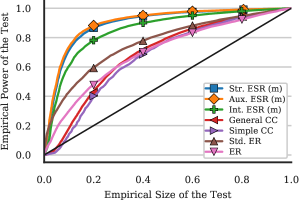
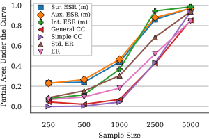
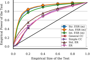
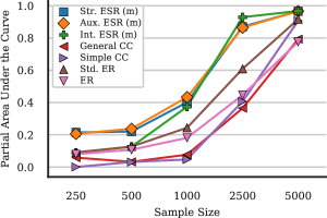
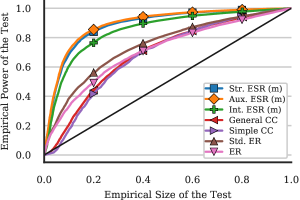

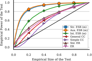
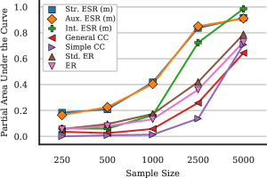
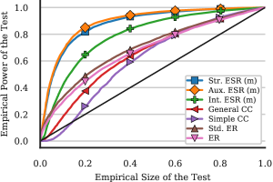
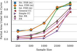
The left panels in Figure 1 and Figure 2 contain the size-adjusted power of the backtests for all empirical sizes in the unit interval for a sample size of 1000 and for the different DGPs.777 These plots are known as the receiver operating characteristic (ROC) curves and origin from the psychometrics literature (Lloyd, , 2005). They are an effective presentation method for general binary classification tasks such as hypothesis testing as they show the size-adjusted power simultaneously for all significance levels. The black line depicts the case of equal empirical size and power, which can be seen as a lower bound for any reasonable test: whenever the power is below this line, randomly guessing the test decision is more accurate than performing the test. For the three ESR backtests, we only report power for the tests relying on the misspecification robust covariance estimator as these versions of the tests exhibit superior size properties for all considered DGPs. We observe that throughout all six considered DGPs, the three ESR backtests clearly dominate the four competitors in terms of power at almost all empirical sizes, including the most relevant region of test sizes between 1% and 10%. Especially the Strict and the Auxiliary ESR tests exhibit a substantially larger power.
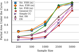
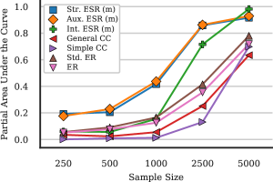
In order to present results for all considered sample sizes in condensed form for the relevant area of empirical sizes between 1% and 10%, we summarize the size-adjusted power by the partial area under the curve (PAUC), as proposed by Lloyd, (2005). For that, we numerically compute the area under each power curve for the empirical sizes between 1% and 10%, which can be interpreted as the test power averaged over the different test sizes. In the right-hand panels of Figure 1 and Figure 2, we present the PAUC for all backtests, DGPs and sample sizes. As expected, the average power increases with the sample size, so that using more information leads to more reliable decisions about the quality of a forecast. We find that for all considered sample sizes, the ESR backtests dominate the other testing approaches. This dominance is especially pronounced for the Strict and the Auxiliary ESR tests. The almost identical performance of the Strict and the Auxiliary ESR tests throughout all simulation designs in Figure 1 and Figure 2 emphasizes that the misspecification introduced by the Strict ESR test seems to be unproblematic for realistic financial data.
3.2 Continuous Model Misspecification
In the second simulation study, we use a GARCH(1,1) model with standardized Student- distributed innovations,
| (3.8) | ||||
with the parameter values , , , and for the true model. For the analysis of the backtests, we simulate 10,000 times from this model with a fixed sample size of 2500 observations and consider the probability level for the VaR and the ES.
|
|
|
|
|
|
|
|
|
|
|
||||||||||||||||||||
|---|---|---|---|---|---|---|---|---|---|---|---|---|---|---|---|---|---|---|---|---|---|---|---|---|---|---|---|---|---|---|
| Misspec Covariance | Classical Covariance | |||||||||||||||||||||||||||||
| Two-Sided | 0.07 | 0.07 | 0.06 | 0.05 | 0.05 | 0.06 | 0.07 | 0.09 | 0.05 | 0.05 | ||||||||||||||||||||
| One-Sided | – | – | 0.03 | – | – | 0.03 | 0.02 | 0.03 | 0.06 | 0.06 | ||||||||||||||||||||
| Notes: This table shows the empirical sizes of the backtests for the GARCH(1,1)- model given in (3.8), for a nominal test size of 5% and for both, one-sided and two-sided hypotheses. The number of Monte-Carlo repetitions is 10,000 and the probability level for the risk measures is . ESR refers to the backtests introduced in this paper. CC refers to the conditional calibration tests of Nolde and Ziegel, (2017), and ER to the exceedance residuals tests of McNeil and Frey, (2000). Note that the Strict and Auxiliary ESR tests do not permit testing against a one-sided alternative and therefore, we only present sizes for the two-sided hypothesis. | ||||||||||||||||||||||||||||||
Table 2 presents the empirical sizes of the backtests for a nominal size of 5% for both, the two- and one-sided hypotheses. As in the first simulation study, we find that most of the backtests are reasonably sized with rejection frequencies close to the nominal value.
For a detailed analysis of the power of the backtests, we continuously misspecify the true model according to the following five designs:
-
(a)
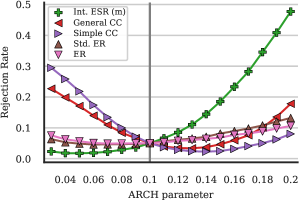
We misspecify how the conditional variance reacts to the squared returns by varying the ARCH parameter . We choose between 0.03 and 0.2 and let , such that the persistence of the GARCH process remains constant. When , there is too little variation in the ES forecasts due to the reduced response to shocks and the GARCH process approaches a constant volatility model.
-
(b)
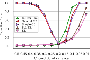
We alter the unconditional variance of the GARCH process between and by varying the parameter while holding and constant. Since the conditional variance is a weighted combination of the unconditional variance, the past squared returns and the past conditional variance, this change implies that the ES forecasts are too conservative when the unconditional variance is larger than its true value, and vice versa.
-
(c)
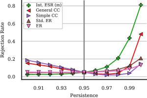
We vary the persistence of shocks between and by setting and for a varying constant and by setting in order to stabilize the unconditional variance. A higher persistence causes a stronger and longer reaction to shocks.
-
(d)
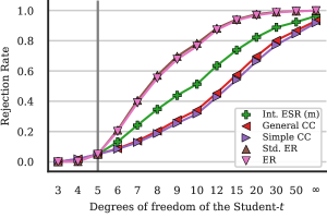
We vary the degrees of freedom of the underlying Student- distribution between 3 and . Since the conditional variance is unaffected, this modification implies a relative horizontal shift of the ES forecasts.
-
(e)
We misspecify the probability level of the ES forecasts between and . This represents the scenario that a forecaster submits (accidentally or on purpose) predictions for some level . Similar to changing the degrees of freedom, this modification implies a relative horizontal shift of the ES forecasts.
As an illustrative example of these misspecifications, Figures 4(a), 4(b), 4(c), 4(d) and 4(e) in Appendix C depict 250 realizations of the returns of the true DGP in (3.8), together with the corresponding ES forecasts of the true model (black dashed line) and of two exemplary models following the parameter misspecifications described in the points (a) to (e) above.
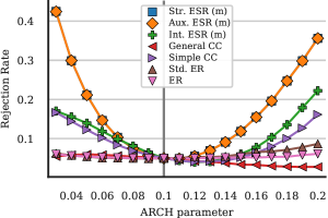
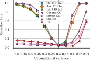
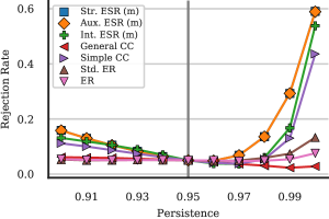
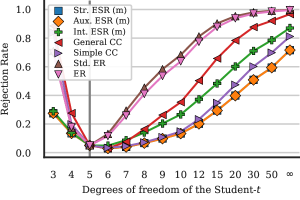
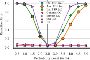
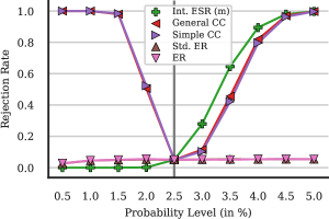
We present the size-adjusted rejection rates plotted against the respective misspecified parameters for these five designs in Figures 2(a), 2(b), 2(c), 2(d) and 2(e). The true model is indicated by the gray vertical line and, induced by the results of Section 3.1 in Appendix C, the x-axis is oriented such that too risky (too small in absolute value) ES forecasts are on the right side of the true model.888Notice that this inequality of the forecast magnitude only holds on average in the cases of Figures 2(a) and 2(c) whereas it holds strictly for Figures 2(b), 2(d) and 2(e). Even though there is no backtest that dominates the others throughout all considered designs, several conclusions can be drawn from this figure.
(1) Overall, the Strict and Auxiliary ESR tests perform almost indistinguishable and in four out of the five considered designs, their performance is superior compared to the general CC and both ER backtesting approaches. (Figures 2(a), 2(b), 2(c) and 2(e)). The ESR backtests outperform the competitors especially when we misspecify the volatility dynamics of the underlying GARCH process (Figures 2(a), 2(b) and 2(c)). This shows that, in contrast to the existing approaches, our ESR backtests can be used to detect misspecifications in the dynamics used to construct the ES forecasts which go beyond level shifts.
(2) The two ER tests (and the general CC test that is constructed to be similar to the ER backtest) can hardly discriminate between forecasts for the VaR and ES issued through misspecified volatility processes (Figures 2(a), 2(b) and 2(c)) and through misspecified probability levels (Figure 2(e)). This confirms the theoretical results discussed in Section B.1 in Appendix B that these backtests only reject misspecifications which affect the relation (distance) between the VaR and ES forecasts. In contrast, these backtests perform well in the case of misspecified tails of the residual distribution, which particularly affects the relative distance between the VaR and ES forecasts (Figure 2(d)). If these backtests would be used by the regulatory authorities, banks could submit joint VaR and ES forecasts for some level or some (too small) volatility process in order to minimize their capital requirements without facing the risk of being detected by these backtests. In comparison, our Intercept ESR backtest which is similar to the ER backtests by construction is clearly able to identify these misspecified probability levels.
(3) Throughout all five misspecifications, the simple CC backtest also exhibits good power properties, similar to our proposed backtests. However, our three ESR backtests exhibit much better size properties (see Section 3.1 and Table 2) and in contrast to the simple CC test, they do not fail to reject the HS forecasts in the first simulation study (see Figure 1).
Together with the results from the first simulation study, these findings demonstrate that our proposed ESR backtests are a powerful choice for backtesting ES forecasts. They are reasonably sized and exhibit good power properties against a variety of misspecifications. Notably, in contrast to the existing backtests, there is no single type of misspecification where our ESR tests are unable to discriminate between forecasts of the true and the misspecified models.
3.3 Testing One-Sided Hypotheses
For the regulatory authorities, testing against a one-sided alternative might be more meaningful than the two-sided versions of the tests we consider in the previous sections. Holding more money than stipulated bv the Basel Accords is no concern for regulators as it is only important that banks keep enough monetary reserves to cover the risks from their market activities. In the following, we assess the performance of the Intercept ESR backtest and the one-sided versions of the four competitor backtests in rejecting the null hypothesis that the issued ES forecasts are at least as conservative (not smaller in absolute value) as the true ES, i.e. that the associated market risk is not underestimated.
In Figures 3(a), 3(b), 3(c), 3(d) and 3(e), we present the size-adjusted rejection rates for the one-sided versions of the considered backtests and for the five continuous parameter misspecifications described in the points (a) - (e) from the previous section. The structure of these figures is analog to the two-sided case where the x-axis is oriented such that too risky ES forecasts are on the right side of the true model (vertical gray line). As it can be seen in Figures 4(a), 4(b), 4(c), 4(d) and 4(e) in Appendix C, the five modifications of the true model exhibit clear patterns when they issue too risky, respectively too conservative forecasts for the true ES, where this finding holds strictly for the cases (b), (d) and (e) and on average for the cases (a) and (c). Thus, the one-sided backtests should only reject the null hypothesis for ES forecasts that issue too risky (too small in absolute value) forecasts, i.e. which are on the right side of the true model in Figures 3(a), 3(b), 3(c), 3(d) and 3(e).
We find that our Intercept ESR backtest is reasonably sized (compare Table 2) and clearly dominates the ER and the CC tests in terms of their power in four out of the five misspecification designs. Only when altering the degrees of freedom, the ER tests are slightly more powerful than the Intercept ESR test. Surprisingly, we see that in four out of the five cases, the one-sided CC tests (both, the simple and the general version) also reject too conservative ES forecasts, even though these should not be rejected by the specifications of the one-sided tests. Furthermore, as for the two-sided tests, both ER backtests fail to detect misspecifications of the underlying volatility process and of the underlying probability level. Summarizing these results, the proposed Intercept ESR backtest is a powerful backtest with good size properties for testing one-sided hypotheses which clearly dominates the existing one-sided (joint VaR and ES) backtesting techniques in the literature.
4 Empirical Application
In the empirical application we apply our backtests to compare ES forecasts along three dimensions: the complexity of the risk model, the length of the estimation window, and the model refit frequency. From a practitioners point of view, it would be desirable to have a parsimonious model that can be estimated with few observations and is valid over a long period of time, for reasons of low engineering effort, data storage, and human and computational effort for updating the model. To assess whether such a setup is reasonable, and if not, which dimensions are crucial for a good performance, we compare rejection rates of ES forecasts using our backtests.
For this application, we use daily log returns of the 200 most highly capitalized stocks of the S&P 500 index (as of September 1, 2019), with a sufficiently long history of stock prices. We consider four different risk models: the standard GARCH(1,1) of Bollerslev, (1986) and the GJR-GARCH(1,1) model of Glosten et al., (1993), both coupled with Gaussian and Student- distributed innovations. For all four models and 200 stocks, we compare the same evaluation horizon, the period from January 2010 to August 2019 with a total of 2432 daily observations. We furthermore consider five different lengths of the rolling estimation window ranging from one year (250 trading days) up to eight years (2000 trading days) and refit horizons of 5, 21, 62, 125 and 250 days, corresponding to weekly, monthly, quarterly, bi-yearly and yearly updating of the models.
Section 4 presents the rejection rates of the one-sided intercept ESR backtest with a nominal size of for the 200 stocks under investigation, for the four GARCH specifications, the five estimation window sizes and the five refit frequencies. We choose to use the one-sided intercept test as this is the only one-sided and strict ES backtest in the literature. Given the currently implemented traffic light system of the Basel Committee, this one-sided test might be the one with the highest practical relevance for backtesting the ES.
& GARCH- GJR-GARCH- 250 0.26 0.32 0.32 0.36 0.59 0.28 0.32 0.29 0.37 0.42 500 0.10 0.09 0.12 0.12 0.20 0.13 0.17 0.17 0.22 0.25 1000 0.07 0.07 0.07 0.08 0.09 0.14 0.11 0.11 0.12 0.14 1500 0.09 0.09 0.09 0.10 0.09 0.08 0.10 0.09 0.09 0.09 2000 0.10 0.08 0.08 0.08 0.09 0.09 0.09 0.10 0.09 0.10
Notes: This tables shows the rejection rates of the one-sided ESR backtest for ES forecasts stemming from the two GARCH-type models with Student’s and Gaussian residuals, different rolling window sizes and model refit lengths (in days). The rejection frequencies are averaged over the analyzed 200 most capitalized stocks of the S&P 500 index. The out-of-sample window covers the time from Jan. 2010 to Aug. 2019 resulting in a sample size of 2432 days.
The results show that both, the GARCH- and GJR-GARCH- are rejected for almost all the stocks (in more than 94% of the cases) uniformly over the different estimation sample sizes and refit frequencies. Independent of the sample length and refit frequency, this supports the well known finding that Gaussian residuals generally fail to capture the riskiness of financial assets, especially in the tail of the distribution. In contrast, for the two GARCH specifications with Student- distributed innovations, the rejection frequencies are considerably lower and for many choices of refit frequencies and estimation windows, they are just above the nominal significance level. These results imply that using fat-tailed distributions generally decreases the rejection frequency. Similarly, refitting the models more frequently tends to decrease the rejection frequency, especially if the estimation window is short. However, refitting the model on a monthly or even weekly basis is not required, infrequent regular updates (such as quarterly) suffice, as more frequent updates do not improve performance if the estimation window is large enough. Interestingly, employing the GJR-GARCH model, which accounts for a potential leverage effect in the volatility, does not perform better than the standard GARCH model.
Generally, refitting these models at least quarterly using data which goes at least four years into the past suffices to obtain rejection rates uniformly below . The results of this application, which are diversified over 200 individual stocks, indicate that in order to obtain satisfactory ES forecasts, one should use fat-tailed residual distributions, more than four years of data and regular refitting of the models at least once per quarter.
5 Conclusion
With the upcoming implementation of the third Basel Accords, risk managers and regulators will shift attention to the risk measure Expected Shortfall (ES) for the forecasting and evaluation of financial risks. In this paper, we introduce regression based ESR backtests for ES forecasts, which extend the classical Mincer and Zarnowitz, (1969) test to ES specific versions. As estimation of regression parameters for the ES stand-alone is infeasible, our tests build on a recently developed joint VaR and ES regression, which allows for different specifications of our tests, titled the Auxiliary, Strict, and Intercept ESR backtests. As these tests are potentially subject to model misspecification, we extend the asymptotic theory for the joint VaR and ES regression framework to possibly misspecified models and verify the tests’ performance in finite samples through an extensive simulation study. We apply our tests to 200 stocks from the S&P 500 index in order to analyze the performance of ES forecasts stemming from the GARCH model family. We find that using fat-tailed (Student’s ) residual distributions, more than four years of data and regular refitting of the models at least once per quarter yields satisfactory ES forecasts.
A unique and essential feature of the Strict and Intercept ESR backtests is that they solely require forecasts for the ES and are consequently the first backtests for the ES stand-alone. In contrast, a common drawback of the existing backtests in the literature is that they need forecasts of further input parameters, such as the VaR, the volatility, the tail distribution or even the whole return distribution. Using more information than the ES forecasts is problematic for two reasons. First, these tests are not applicable for the regulatory authorities, who receive forecasts of the ES, but not of the additional information required by these tests. Second, rejecting the null hypothesis does not necessarily imply that the ES forecasts are incorrect as the rejection can be a result of a false prediction of any of the input parameters.
This paper contributes to the ongoing discussion about which risk measure is the best in practice in the following way. As the VaR is criticized for not being subadditive and for not capturing tail risks beyond itself, the recent literature proposes both, the ES and expectiles as alternative risk measures. Expectiles are suggested as they are coherent, elicitable and are able to capture extreme risks beyond the VaR and thus, they simultaneously overcome the drawbacks of the VaR and the ES (Bellini et al., , 2014; Ziegel, , 2016). Unfortunately, as opposed to the VaR and ES, they lack a visual and intuitive interpretation (Emmer et al., , 2015). In contrast, the ES is mainly criticized for its theoretical deficiencies of being not elicitable and not (only with difficulties) backtestable. However, starting with the joint elicitability result of VaR and ES of Fissler and Ziegel, (2016), there is a growing body of literature using this result for a regression procedure (Dimitriadis and Bayer, , 2019; Barendse, , 2018; Patton et al., 2019a, ) and for relative forecast comparison (Fissler et al., , 2016; Nolde and Ziegel, , 2017), which is extended by this paper through introducing the ESR backtests, which are the first sensible backtests for the ES stand-alone. This shows that, even though technically more demanding, the ES can be modeled, evaluated and backtested in the same way as quantiles and expectiles. Combining this with its ability to capture extreme tail risks and its intuitive visual interpretation, the ES is an appropriate candidate for being the standard risk measure in practice.
Acknowledgments
We thank the editor Andrew Patton, an anonymous associate editor and two referees for very helpful comments. We further thank Tobias Fissler, Lyudmila Grigoryeva, Roxana Halbleib, Phillip Heiler, Ekaterina Kazak, Winfried Pohlmeier, James Taylor, and Johanna Ziegel for suggestions which inspired some results of this paper. Financial support by the Heidelberg Academy of Sciences and Humanities (HAW) within the project “Analyzing, Measuring and Forecasting Financial Risks by means of High-Frequency Data” and by the German Research Foundation (DFG) within the research group “Robust Risk Measures in Real Time Settings” is gratefully acknowledged. The authors acknowledge support by the state of Baden-Württemberg through bwHPC. The majority of the work on this paper was conducted while both authors were at the Department of Economics, Universität Konstanz.
Appendix A Proofs
Proof of Theorem 2.3.
We check that the necessary conditions (i) - (iv) of the basic consistency theorem, given in Theorem 2.1 in Newey and McFadden, (1994), p.2121 hold, where we consider the objective functions and as defined in (2.17) and (2.19). First, notice that condition (ii) holds by imposing condition (A2). The unique identification condition (i) holds by assumption (A3). Next, we verify the uniform convergence condition (iv) by applying the uniform weak law of large numbers given in Theorem A.2.5. in White, (1994). For that, we have to show that
- (A)
-
(B)
For all , there exists , such that for all , the sequences
(A.1) (A.2) obey a weak law of large numbers.
Condition (A) follows directly from Lemma A.1 and we turn to condition (B). As the process is strong mixing of size for some by condition (A6), the processes and are strong mixing of the same size by Theorem 3.49 in White, (2001), p. 50. As the functions and the supremum/infimum functions are -measureable for all , we can conclude that the sequences and are also strong mixing of the same size by applying the same theorem.
Furthermore, for and for some sufficiently small enough, and thus for all . As is compact, there exists some such that and thus, for all , it holds that
| (A.3) |
which is bounded by condition (A8) and as for large enough. The same inequality holds for . Thus, we can apply the weak law of large numbers for strong mixing sequences in Corollary 3.48 in White, (2001), p. 49 in order to conclude that for all such that , it holds that and , which shows condition (B). Consequently, the uniform convergence condition (iv) holds by applying the uniform weak law of large numbers given in Theorem A.2.5. in White, (1994).
Proof of Theorem 2.4.
Let
| (A.4) |
which is almost surely the derivative of with respect to . We further define and . From the proof of Lemma A.2, we get the mean value expansion (for close to ),
| (A.5) |
for some values and somewhere on the line between and , where the components of are given in (A.8) and (A.9), and where .101010The mean-value theorem cannot be generalized in a straight-forward fashion to vector-valued functions. Thus, we have to consider the mean value expansion in each component separately which gives this more complicated expression.
Furthermore, it holds that and is a continuous function in its arguments and . Using that has Eigenvalues bounded away from zero (for large enough), we also get that is non-singular in a neighborhood around (for all arguments) for large enough as the map which maps the matrix onto its Eigenvalues is continuous. As we further know that and for all , we get from the continuous mapping theorem that
| (A.6) |
In the following, we apply Lemma A.1 in Weiss, (1991) (by verifying its assumptions), which extends the iid results of Huber, (1967) to strong mixing sequences. Assumption (N1) of Lemma A.1 in Weiss, (1991) is satisfied as every almost surely continuous stochastic process is separable in the sense of Doob (Gikhman and Skorokhod, , 2004) and the functions are almost surely continuous for all . Assumption (N2) is satisfied as shown in the proof of Theorem 2.3. Assumption (N3)(i) is shown in Lemma A.2. The technical Assumptions (N3)(ii) and (N3)(iii) follow from Lemma 4 and Lemma 5 in Patton et al., 2019b . For this, notice that the moment conditions in Assumption 2 (C) and (D) of Patton et al., 2019a are implied by the condition (A8) in Assumption 2.2 for the simplified case of linear models. Assumption (N4) follows from the moment conditions (A8) in Assumption 2.2 and Assumption (N5) from the strong mixing condition (A6). Furthermore, Lemma 2 of Patton et al., 2019b implies that . Thus, we can apply Lemma A.1 in Weiss, (1991) and get that
| (A.7) |
Combining (A.5), (A.6) and (A.7), we get that
| (A.8) | ||||
| (A.9) | ||||
| (A.10) |
Furthermore,
| (A.11) |
by Lemma A.3 and thus,
| (A.12) |
which concludes the proof of this theorem. ∎
SUPPLEMENTARY MATERIAL
Appendix A Technical Proofs
Lemma A.1.
Given the conditions from Assumption 2.2, the function is -Lipschitz on with -measurable and integrable Lipschitz-constant.
Proof.
We split the -function , where
Local Lipschitz continuity of follows since it is a continuously differentiable function in (such that ) and thus (locally) Lipschitz-. We consequently get that for all , there exists a such that for all , it holds that
| (A.1) |
where the sequences and are bounded for all by the conditions (A7) and (A8) in Assumption 2.2.
For the function , we consider four cases. First, let . Then, on , it holds that,
| (A.2) |
which is obviously Lipschitz-.
Lemma A.2.
Given the conditions from Assumption 2.2, there exist constants such that
| (A.5) |
and for all , where is large enough.
Proof.
Let such that for some (small) constant and define
| (A.6) | ||||
| (A.7) |
such that . Then, by applying the mean-value theorem we get that
| (A.8) |
for some on the line between and . Equivalently, for the second component,
| (A.9) |
for some on the line between and . Notice that and are not necessarily the same as the mean-value theorem does not hold in its classical form for vector-valued functions. Thus, for , we get that
| (A.10) |
In the following, we show that . For the first component of , we get that
| (A.11) | ||||
| (A.12) |
for some on the line between and .
For the second component of (and equivalently for the first component of of ), we get that
| (A.13) | ||||
| (A.14) |
for some on the line between and .
Eventually, for the second component of , we get that
| (A.15) | ||||
| (A.16) | ||||
| (A.17) |
for some on the line between and . As the respective moments are finite given the moment conditions in (A8) in Assumption 2.2 and since and , we have shown that for all sufficiently large enough, there exists a constant such that
| (A.18) |
Furthermore, as the matrix has Eigenvalues bounded from below (for large enough) by assumption, there exists a constant , such that
| (A.19) |
Thus, we choose small enough such that . Then and thus, . Consequently, and thus
| (A.20) | ||||
| (A.21) | ||||
| (A.22) | ||||
| (A.23) |
by applying the mean value expansion and the inverse triangular inequality. ∎
Lemma A.3.
Given Assumption 2.2, it holds that
| (A.24) |
Proof.
We show this multivariate result by applying the Cramér–Wold theorem, i.e. by showing that the conditions for the univariate CLT for -mixing sequences given in Theorem 5.20 in White, (2001), p.130 hold for all linear combinations for all such that . By Theorem 3.49 in White, (2001) p.50, we get that the sequences and are strong mixing of size for some . Furthermore, for all , it holds that
by applying Jensen’s inequality and by the moment conditions (A8) in Assumption 2.2, where (from condition (A6)). As the sequence is uncorrelated by condition (A3) in Assumption 2.2, we get that for all ,
| (A.25) |
As is real and symmetric and positive definite, it can be diagonalized with a real orthogonal matrix , i.e. , where is a diagonal matrix containing the Eigenvalues of , denoted by . Consequently, for any ,
| (A.26) |
where , i.e. as is orthogonal and where the Eigenvalues are bounded away from zero for sufficiently large. Thus, we can apply Theorem 5.20 in White, (2001) p. 130 for asymptotic normality of the sequences for all such that . Applying the Cramér-Wold theorem concludes the proof. ∎
Appendix B Existing Backtests
Over the past two decades and especially driven by the recent transition from VaR to ES in the Basel regulatory framework (Basel Committee, , 2016, 2017), a large literature on backtesting the ES has emerged. These backtests are usually introduced with financial regulators in mind who need to verify the risk forecasts they receive from the financial institutions. To be applicable by the regulatory authorities, a backtest for the risk measure ES thus follows Definition 2.1 and only requires the observed return series and the ES forecasts as input variables. However, many of the proposed backtests for the ES fail to have this property. In particular, several tests require the whole return distribution (or equivalently the cumulative violation process ) (Kerkhof and Melenberg, , 2004; Wong, , 2008; Graham and Pál, , 2014; Acerbi and Szekely, , 2014; Du and Escanciano, , 2017; Löser et al., , 2018; Costanzino and Curran, , 2018), multiple quntile levels (Emmer et al., , 2015; Costanzino and Curran, , 2015; Kratz et al., , 2018; Couperier and Leymarie, , 2019), the VaR and the volatility (McNeil and Frey, , 2000; Nolde and Ziegel, , 2017; Righi and Ceretta, , 2013, 2015), or the VaR (McNeil and Frey, , 2000; Nolde and Ziegel, , 2017) in addition to the ES forecasts. However, this information is not reported by the financial institutions and therefore, most of these tests can not be used by the regulators (Aramonte et al., , 2011; Basel Committee, , 2017).
Furthermore, when more information than solely the ES forecasts is used for backtesting, a rejection of the null hypothesis does not necessarily imply that the ES forecasts are wrong. More precisely, a rejection of the null implies that some component of the input parameters is incorrect (cf. Nolde and Ziegel, , 2017). A related concern is raised by Aramonte et al., (2011), who note that financial institutions could be tempted to submit forecasts of this additional information chosen such that the tests have particularly low power, so that correctness of their internal model (and their issued ES forecasts) is not doubted.
Strictly following Definition 2.1, we would have to distinguish between backtests for the ES and joint backtests for the pair VaR and ES. However, as the ES is strongly intertwined with the VaR (through its definition and through the joint elicitability), sensible forecasts for the ES are based on correctly specified VaR forecasts. Consequently, it is reasonable to backtest both quantities jointly and thus, we compare the performance of our ESR backtests to existing joint VaR and ES backtests in the literature. In the subsequent two sections, we describe the exceedance residual (ER) backtests of McNeil and Frey, (2000) and the conditional calibration (CC) backtests of Nolde and Ziegel, (2017) in detail, since both have versions that only require VaR forecasts in addition to the ES.
B.1 Testing the Exceedance Residuals
One of the first and still most frequently used tests for the ES is the exceedance residual (ER) backtest of McNeil and Frey, (2000). This approach is based on the ES-specified residuals that exceed the VaR, , which form a martingale difference sequence given that and are the true quantile and ES conditional on the information . McNeil and Frey, (2000) further consider a second version that uses exceedance residuals standardized by a given volatility forecast, i.e. .
This backtest tests whether the expected value of the (raw or standardized) ER, , is zero using the estimate in conjunction with a bootstrap hypothesis test (see Efron and Tibshirani, , 1994, p. 224). In the original paper, McNeil and Frey, (2000) propose to test against the one-sided alternative that is negative, i.e. that the issued ES forecasts are too risky (too small in absolute value). However, in this paper we discuss both, tests based on one-sided and two-sided hypotheses, so that in addition to the original proposal, we also include a two-sided test,
| (B.1) | ||||
By Definition 2.1, the test using the standardized ER is in fact a joint backtest for the triple VaR, ES and volatility, whereas the test using the raw ER is a joint backtest for the pair VaR and ES. In light of the discussion above, the test using the raw ER is therefore preferred. Nevertheless, in the simulation studies and the empirical application we apply both approaches and find that they perform alike.
Even though the intercept ESR test introduced in Section 2.3 and the ER backtest appear to be similar, there is a subtle but crucial difference between the two test statistics. For the intercept ESR test, we compute the empirical ES of , i.e. the average of given that is smaller than its empirical -quantile. In contrast, the ER backtest computes the average of , given that is smaller than the respective forecast for its -quantile . This difference seems marginal, but it has severe consequences for the theoretical and empirical properties of the tests.
As we can write , where , the ER backtest in fact compares the empirical average of truncated at to the average ES forecast , whenever there is a VaR violation. Thus, this backtest rejects whenever the distance/relation between the VaR and ES-forecasts is incorrect. However, simultaneous misspecifications of both forecasts, such as e.g. generated by misspecification of the volatility process in location scale models cannot be detected. In the same spirit, the ER backtest cannot distinguish between correct forecasts for the VaR and ES at level and (correct) forecasts for a misspecified probability level , as the given level does not influence the ER test statistic at all. In contrast, by computing the empirical -quantile of (instead of using the forecast ), the intercept ESR test does not suffer from these shortcomings as can be observed in the simulation results in Section 3.2.
B.2 Conditional Calibration Backtests
Nolde and Ziegel, (2017) introduce the concept of conditional calibration (CC) based on strict identification functions (also known as moment conditions or estimating equations) of the respective functional and show that many classical backtests for risk measures can be unified using this concept. For the pair VaR and ES at level , they choose the strict identification function
| (B.2) |
whose expectation is zero if and only if and equal the true VaR and ES of the random variable respectively. The CC backtest for forecasts for the VaR, and for the ES, is based on the hypotheses
| (B.3) | ||||
component-wise and almost surely for all . This is equivalent to testing for all measurable -valued functions . As this is infeasible, Nolde and Ziegel, (2017) propose to use an -measurable sequence of -matrices of test functions for some and to use the Wald-type test statistic
| (B.4) |
where is a consistent estimator of the covariance of the -dimensional vector . Under , the test statistic asymptotically follows a distribution with degrees of freedom.
Nolde and Ziegel, (2017) propose two versions of this test, where the first uses no information besides the risk forecasts (termed simple CC test), and where the second additionally requires volatility forecasts (termed general CC test). For the simple CC test, the test function is the identity matrix, for both, the one- and two-sided hypotheses. For the general CC test, they propose to choose
| (B.5) |
for the two-sided and for the one-sided test, respectively, where is a forecast for the volatility. As with the standardized ER test, the general CC test is strictly speaking a backtest for the triple VaR, ES, and volatility, but we nevertheless include both versions in our empirical comparisons. We provide implementations of the two ESR backtests proposed in this paper, both ER backtests of McNeil and Frey, (2000) and both CC backtests of Nolde and Ziegel, (2017) in the R package esback (Bayer and Dimitriadis, 2019a, ).
Appendix C Additional Material
|
|
|
|
|
|
|
|
|
|
|
|
||||||||||||||||||||||
|---|---|---|---|---|---|---|---|---|---|---|---|---|---|---|---|---|---|---|---|---|---|---|---|---|---|---|---|---|---|---|---|---|---|
| Misspec Covariance | Classical Covariance | ||||||||||||||||||||||||||||||||
| 250 | 0.05 | 0.05 | 0.09 | 0.16 | 0.16 | 0.10 | 0.01 | 0.22 | 0.04 | 0.05 | |||||||||||||||||||||||
| 500 | 0.03 | 0.03 | 0.05 | 0.08 | 0.08 | 0.06 | 0.03 | 0.13 | 0.01 | 0.01 | |||||||||||||||||||||||
| EGARCH-STD | 1000 | 0.02 | 0.02 | 0.03 | 0.05 | 0.05 | 0.03 | 0.04 | 0.08 | 0.01 | 0.02 | ||||||||||||||||||||||
| 2500 | 0.01 | 0.01 | 0.01 | 0.02 | 0.02 | 0.01 | 0.02 | 0.04 | 0.01 | 0.01 | |||||||||||||||||||||||
| 5000 | 0.01 | 0.01 | 0.01 | 0.02 | 0.01 | 0.01 | 0.02 | 0.03 | 0.01 | 0.01 | |||||||||||||||||||||||
250 0.05 0.06 0.08 0.17 0.17 0.10 0.01 0.21 0.04 0.05 500 0.04 0.04 0.06 0.09 0.09 0.06 0.02 0.13 0.01 0.01 GAS-STD 1000 0.02 0.02 0.03 0.06 0.06 0.03 0.03 0.08 0.02 0.02 2500 0.01 0.02 0.01 0.03 0.03 0.01 0.02 0.05 0.01 0.01 5000 0.01 0.01 0.01 0.02 0.02 0.01 0.02 0.03 0.01 0.01 250 0.05 0.05 0.08 0.16 0.16 0.09 0.01 0.20 0.04 0.04 500 0.03 0.03 0.05 0.08 0.08 0.06 0.02 0.12 0.01 0.01 GAS-SSTD 1000 0.02 0.02 0.03 0.04 0.04 0.03 0.03 0.07 0.02 0.01 2500 0.01 0.01 0.01 0.02 0.02 0.01 0.02 0.04 0.01 0.01 5000 0.01 0.01 0.01 0.01 0.01 0.01 0.02 0.03 0.02 0.01 250 0.02 0.02 0.06 0.10 0.10 0.07 0.01 0.17 0.04 0.04 500 0.02 0.02 0.04 0.05 0.05 0.05 0.02 0.09 0.00 0.00 AR-GARCH, 1000 0.01 0.01 0.03 0.04 0.04 0.03 0.02 0.05 0.00 0.01 2500 0.01 0.01 0.02 0.02 0.02 0.02 0.02 0.03 0.01 0.01 5000 0.01 0.01 0.01 0.02 0.02 0.01 0.01 0.02 0.01 0.01 250 0.02 0.02 0.06 0.10 0.10 0.07 0.01 0.17 0.04 0.04 500 0.02 0.02 0.04 0.05 0.05 0.05 0.02 0.09 0.00 0.00 AR-GARCH, 1000 0.01 0.01 0.03 0.03 0.04 0.03 0.02 0.05 0.00 0.01 2500 0.01 0.01 0.02 0.02 0.02 0.02 0.02 0.03 0.01 0.01 5000 0.01 0.01 0.01 0.01 0.02 0.01 0.01 0.02 0.01 0.01 250 0.02 0.02 0.06 0.09 0.09 0.07 0.01 0.17 0.04 0.04 500 0.02 0.02 0.04 0.06 0.06 0.04 0.02 0.09 0.00 0.00 AR-GARCH, 1000 0.01 0.01 0.03 0.04 0.04 0.03 0.02 0.05 0.00 0.01 2500 0.01 0.01 0.02 0.02 0.02 0.02 0.02 0.03 0.01 0.01 5000 0.01 0.01 0.01 0.02 0.02 0.01 0.01 0.02 0.01 0.01 Notes: The table reports the empirical sizes of the backtests for the different DGPs decribed in Section 3.1 and for a nominal test size of . The number of Monte-Carlo repetitions is 10,000 and the probability level for the risk measures is . ESR refers to the three backtests introduced in this paper and we consider versions with covariance estimation with and without model misspecification. CC refers to the conditional calibration tests of Nolde and Ziegel, (2017), and ER to the exceedance residuals tests of McNeil and Frey, (2000).
|
|
|
|
|
|
|
|
|
|
|
|
||||||||||||||||||||||
|---|---|---|---|---|---|---|---|---|---|---|---|---|---|---|---|---|---|---|---|---|---|---|---|---|---|---|---|---|---|---|---|---|---|
| Misspec Covariance | Classical Covariance | ||||||||||||||||||||||||||||||||
| 250 | 0.12 | 0.12 | 0.19 | 0.31 | 0.31 | 0.20 | 0.16 | 0.33 | 0.12 | 0.14 | |||||||||||||||||||||||
| 500 | 0.09 | 0.09 | 0.15 | 0.21 | 0.21 | 0.16 | 0.16 | 0.25 | 0.10 | 0.12 | |||||||||||||||||||||||
| EGARCH-STD | 1000 | 0.08 | 0.08 | 0.13 | 0.16 | 0.16 | 0.13 | 0.14 | 0.19 | 0.10 | 0.13 | ||||||||||||||||||||||
| 2500 | 0.08 | 0.08 | 0.11 | 0.11 | 0.12 | 0.11 | 0.12 | 0.14 | 0.10 | 0.11 | |||||||||||||||||||||||
| 5000 | 0.08 | 0.08 | 0.15 | 0.10 | 0.10 | 0.15 | 0.11 | 0.13 | 0.10 | 0.11 | |||||||||||||||||||||||
250 0.14 0.14 0.18 0.32 0.32 0.20 0.15 0.32 0.13 0.13 500 0.11 0.11 0.14 0.22 0.22 0.15 0.15 0.25 0.12 0.12 GAS-STD 1000 0.09 0.09 0.12 0.16 0.16 0.12 0.14 0.19 0.12 0.12 2500 0.09 0.09 0.12 0.13 0.12 0.12 0.12 0.15 0.11 0.12 5000 0.09 0.09 0.17 0.11 0.11 0.17 0.11 0.13 0.11 0.11 250 0.12 0.12 0.17 0.31 0.31 0.19 0.15 0.30 0.14 0.13 500 0.09 0.09 0.14 0.20 0.20 0.15 0.15 0.23 0.12 0.11 GAS-SSTD 1000 0.08 0.08 0.12 0.15 0.15 0.12 0.13 0.18 0.12 0.11 2500 0.07 0.07 0.11 0.11 0.11 0.11 0.13 0.14 0.12 0.10 5000 0.08 0.08 0.13 0.10 0.10 0.13 0.12 0.12 0.11 0.10 250 0.07 0.07 0.16 0.24 0.24 0.18 0.13 0.26 0.11 0.11 500 0.07 0.07 0.14 0.18 0.18 0.15 0.13 0.19 0.08 0.09 AR-GARCH, 1000 0.07 0.07 0.12 0.14 0.14 0.12 0.12 0.16 0.09 0.09 2500 0.07 0.07 0.11 0.11 0.11 0.11 0.11 0.12 0.10 0.10 5000 0.08 0.08 0.11 0.11 0.11 0.11 0.11 0.11 0.10 0.10 250 0.07 0.07 0.16 0.24 0.24 0.18 0.13 0.26 0.11 0.11 500 0.07 0.07 0.14 0.18 0.18 0.15 0.13 0.19 0.08 0.09 AR-GARCH, 1000 0.06 0.07 0.12 0.14 0.14 0.12 0.12 0.16 0.09 0.09 2500 0.07 0.07 0.11 0.11 0.11 0.11 0.11 0.12 0.10 0.10 5000 0.08 0.07 0.11 0.11 0.11 0.11 0.11 0.11 0.10 0.10 250 0.06 0.06 0.16 0.23 0.23 0.18 0.13 0.26 0.11 0.11 500 0.06 0.06 0.14 0.18 0.18 0.15 0.13 0.19 0.08 0.09 AR-GARCH, 1000 0.06 0.06 0.12 0.14 0.14 0.12 0.12 0.16 0.09 0.09 2500 0.07 0.07 0.11 0.12 0.12 0.11 0.11 0.12 0.10 0.10 5000 0.08 0.08 0.11 0.12 0.11 0.11 0.11 0.11 0.10 0.10 Notes: The table reports the empirical sizes of the backtests for the different DGPs decribed in Section 3.1 and for a nominal test size of . The number of Monte-Carlo repetitions is 10,000 and the probability level for the risk measures is . ESR refers to the three backtests introduced in this paper and we consider versions with covariance estimation with and without model misspecification. CC refers to the conditional calibration tests of Nolde and Ziegel, (2017), and ER to the exceedance residuals tests of McNeil and Frey, (2000).
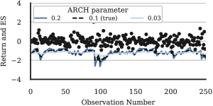
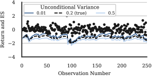
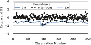

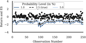
References
- Acerbi and Szekely, (2014) Acerbi, C. and Szekely, B. (2014). Backtesting Expected Shortfall. Risk Magazine, December:76–81.
- Angrist et al., (2006) Angrist, J., Chernozhukov, V., and Fernandez-Val, I. (2006). Quantile regression under misspecification, with an application to the u.s. wage structure. Econometrica, 74(2):539–563.
- Aramonte et al., (2011) Aramonte, S., Durand, P., Kobayashi, S., Kwast, M., Lopez, J. A., Mazzoni, G., Raupach, P., Summer, M., and Wu, J. (2011). Messages from the academic literature on risk measurement for the trading book. Technical report, Bank for International Settlements. Working Paper No. 19, available at http://www.bis.org/publ/bcbs_wp19.pdf.
- Ardia et al., (2019) Ardia, D., Boudt, K., and Catania, L. (2019). Generalized autoregressive score models in r: The gas package. Journal of Statistical Software, Articles, 88(6):1–28.
- Artzner et al., (1999) Artzner, P., Delbaen, F., Eber, J.-M., and Heath, D. (1999). Coherent Measures of Risk. Mathematical Finance, 9(3):203–228.
- Barendse, (2018) Barendse, S. (2018). Interquantile Expectation Regression. Tinbergen Institute Discussion Paper 2017-034/III. Available at https://ssrn.com/abstract=2937665.
- Basel Committee, (1996) Basel Committee (1996). Overview of the Amendment to the Capital Accord to Incorporate Market Risks. Technical report, Bank for International Settlements. Available at http://www.bis.org/publ/bcbs23.pdf.
- Basel Committee, (2013) Basel Committee (2013). Fundamental review of the trading book: A revised market risk framework. Technical report, Bank for International Settlements. Available at http://www.bis.org/publ/bcbs265.pdf.
- Basel Committee, (2016) Basel Committee (2016). Minimum capital requirements for Market Risk. Technical report, Bank for International Settlements. Available at http://www.bis.org/bcbs/publ/d352.pdf.
- Basel Committee, (2017) Basel Committee (2017). Pillar 3 disclosure requirements – consolidated and enhanced framework. Technical report, Basel Committee on Banking Supervision. Available at http://www.bis.org/bcbs/publ/d400.pdf.
- (11) Bayer, S. and Dimitriadis, T. (2019a). esback: Expected Shortfall Backtesting. R package version 0.2.0, available at https://github.com/BayerSe/esback.
- (12) Bayer, S. and Dimitriadis, T. (2019b). esreg: Joint Quantile and Expected Shortfall Regression. R package version 0.4.0, available at https://CRAN.R-project.org/package=esreg.
- Bellini et al., (2014) Bellini, F., Klar, B., Müller, A., and Gianin, E. R. (2014). Generalized quantiles as risk measures. Insurance: Mathematics and Economics, 54(C):41 – 48.
- Bollerslev, (1986) Bollerslev, T. (1986). Generalized autoregressive conditional heteroskedasticity. Journal of Econometrics, 31(3):307–327.
- Carver, (2013) Carver, L. (2013). Mooted VAR substitute cannot be back-tested, says top quant. Risk Magazine, March.
- Cont et al., (2010) Cont, R., Deguest, R., and Scandolo, G. (2010). Robustness and sensitivity analysis of risk measurement procedures. Quantitative Finance, 10(6):593–606.
- Costanzino and Curran, (2015) Costanzino, N. and Curran, M. (2015). Backtesting general spectral risk measures with application to expected shortfall. Risk Magazine, March.
- Costanzino and Curran, (2018) Costanzino, N. and Curran, M. (2018). A simple traffic light approach to backtesting expected shortfall. Risks, 6(1).
- Couperier and Leymarie, (2019) Couperier, O. and Leymarie, J. (2019). Backtesting expected shortfall via multi-quantile regression. available at https://halshs.archives-ouvertes.fr/halshs-01909375v2.
- Creal et al., (2013) Creal, D., Koopman, S. J., and Lucas, A. (2013). Generalized autoregressive score models with applications. Journal of Applied Econometrics, 28(5):777–795.
- Danielsson et al., (2001) Danielsson, J., Embrechts, P., Goodhart, C., Keating, C., Muennich, F., Renault, O., and Shin, H. S. (2001). An Academic Response to Basel II. Financial Markets Group Special Papers, available at https://EconPapers.repec.org/RePEc:fmg:fmgsps:sp130.
- Dimitriadis and Bayer, (2019) Dimitriadis, T. and Bayer, S. (2019). A joint quantile and expected shortfall regression framework. Electron. J. Statist., 13(1):1823–1871.
- Du and Escanciano, (2017) Du, Z. and Escanciano, J. C. (2017). Backtesting Expected Shortfall: Accounting for Tail Risk. Management Science, 63(4):940–958.
- Efron, (1991) Efron, B. (1991). Regression percentiles using asymmetric squared error loss. Statistica Sinica, 1(1):93–125.
- Efron and Tibshirani, (1994) Efron, B. and Tibshirani, R. J. (1994). An Introduction to the Bootstrap. New York: Chapman and Hall.
- Embrechts et al., (2018) Embrechts, P., Liu, H., and Wang, R. (2018). Quantile-based risk sharing. Oper. Res., 66(4):936–949.
- Emmer et al., (2015) Emmer, S., Kratz, M., and Tasche, D. (2015). What Is the Best Risk Measure in Practice? A Comparison of Standard Measures. Journal of Risk, 18(2):31–60.
- Engle and Russell, (1998) Engle, R. F. and Russell, J. R. (1998). Autoregressive conditional duration: A new model for irregularly spaced transaction data. Econometrica, 66(5):1127–1162.
- Fissler and Ziegel, (2016) Fissler, T. and Ziegel, J. F. (2016). Higher order elicitability and Osband’s principle. Annals of Statistics, 44(4):1680–1707.
- Fissler et al., (2016) Fissler, T., Ziegel, J. F., and Gneiting, T. (2016). Expected Shortfall is jointly elicitable with Value at Risk - Implications for backtesting. Risk Magazine, January:58–61.
- Gaglianone et al., (2011) Gaglianone, W. P., Lima, L. R., Linton, O., and Smith, D. R. (2011). Evaluating Value-at-Risk Models via Quantile Regression. Journal of Business & Economic Statistics, 29(1):150–160.
- Gikhman and Skorokhod, (2004) Gikhman, I. and Skorokhod, A. (2004). The Theory of Stochastic Processes I, volume 210 of Classics in Mathematics. Springer Berlin Heidelberg.
- Glosten et al., (1993) Glosten, L. R., Jagannathan, R., and Runkle, D. E. (1993). On the Relation between the Expected Value and the Volatility of the Nominal Excess Return on Stocks. The Journal of Finance, 48(5):1779–1801.
- Gneiting, (2011) Gneiting, T. (2011). Making and Evaluating Point Forecasts. Journal of the American Statistical Association, 106(494):746–762.
- Gourieroux et al., (1984) Gourieroux, C., Monfort, A., and Trognon, A. (1984). Pseudo maximum likelihood methods: Theory. Econometrica, 52(3):681–700.
- Graham and Pál, (2014) Graham, A. and Pál, J. (2014). Backtesting value-at-risk tail losses on a dynamic portfolio. The Journal of Risk Model Validation, 8(2):59.
- Guler et al., (2017) Guler, K., Ng, P. T., and Xiao, Z. (2017). Mincer–Zarnowitz quantile and expectile regressions for forecast evaluations under aysmmetric loss functions. Journal of Forecasting, 36(6):651–679.
- Harvey, (2013) Harvey, A. (2013). Dynamic Models for Volatility and Heavy Tails: With Applications to Financial and Economic Time Series. Econometric Society monographs. Cambridge University Press.
- Hendricks and Koenker, (1992) Hendricks, W. and Koenker, R. (1992). Hierarchical Spline Models for Conditional Quantiles and the Demand for Electricity. Journal of the American Statistical Association, 87(417):58–68.
- Holden and Peel, (1990) Holden, K. and Peel, D. A. (1990). On Testing For Unbiasedness And Efficiency Of Forecasts. The Manchester School, 58(2):120–127.
- Huber, (1967) Huber, P. (1967). The behavior of maximum likelihood estimates under nonstandard conditions. In Proceedings of the Fifth Berkeley Symposium on Mathematical Statistics and Probability, pages 221–233. Berkeley: University of California Press.
- Kerkhof and Melenberg, (2004) Kerkhof, J. and Melenberg, B. (2004). Backtesting for risk-based regulatory capital. Journal of Banking & Finance, 28(8):1845 – 1865.
- Kim and White, (2003) Kim, T.-H. and White, H. (2003). Estimation, inference, and specification testing for possibly misspecified quantile regression. In Maximum Likelihood Estimation of Misspecified Models: Twenty Years Later, pages 107–132. Emerald Group Publishing Limited.
- Koenker and Bassett, (1978) Koenker, R. W. and Bassett, G. (1978). Regression quantiles. Econometrica, 46(1):33–50.
- Komunjer, (2004) Komunjer, I. (2004). Quantile Prediction. In Elliott, G. and Timmermann, A., editors, Handbook of Economic Forecasting, volume 2, chapter 17, pages 961–994. Elsevier.
- Komunjer, (2005) Komunjer, I. (2005). Quasi-maximum likelihood estimation for conditional quantiles. Journal of Econometrics, 128(1):137–164.
- Koopman et al., (2016) Koopman, S. J., Lucas, A., and Scharth, M. (2016). Predicting time-varying parameters with parameter-driven and observation-driven models. Review of Economics and Statistics, 98(1):97–110.
- Kratz et al., (2018) Kratz, M., Lok, Y. H., and McNeil, A. J. (2018). Multinomial VaR backtests: A simple implicit approach to backtesting expected shortfall. Journal of Banking & Finance, 88(C):393–407.
- Lloyd, (2005) Lloyd, C. J. (2005). Estimating test power adjusted for size. Journal of Statistical Computation and Simulation, 75(11):921–933.
- Löser et al., (2018) Löser, R., Wied, D., and Ziggel, D. (2018). New backtests for unconditional coverage of expected shortfall. Journal of Risk, 21(4):1–21.
- McNeil and Frey, (2000) McNeil, A. J. and Frey, R. (2000). Estimation of tail-related risk measures for heteroscedastic financial time series: an extreme value approach. Journal of Empirical Finance, 7(3–4):271–300.
- Mincer and Zarnowitz, (1969) Mincer, J. and Zarnowitz, V. (1969). The Evaluation of Economic Forecasts. In Economic Forecasts and Expectations: Analysis of Forecasting Behavior and Performance, pages 3–46. National Bureau of Economic Research, Inc.
- Nadarajah et al., (2014) Nadarajah, S., Zhang, B., and Chan, S. (2014). Estimation methods for expected shortfall. Quantitative Finance, 14(2):271–291.
- Nelson, (1991) Nelson, D. B. (1991). Conditional Heteroskedasticity in Asset Returns: A New Approach. Econometrica, 59(2):347–370.
- Newey and McFadden, (1994) Newey, W. and McFadden, D. (1994). Large sample estimation and hypothesis testing. In Engle, R. and McFadden, D., editors, Handbook of Econometrics, volume 4, chapter 36, pages 2111–2245. Elsevier.
- Nolde and Ziegel, (2017) Nolde, N. and Ziegel, J. F. (2017). Elicitability and backtesting: Perspectives for banking regulation. The Annals of Applied Statistics, 11(4):1833–1874.
- (57) Patton, A. J., Ziegel, J. F., and Chen, R. (2019a). Dynamic semiparametric models for expected shortfall (and value-at-risk). Journal of Econometrics, 211(2):388 – 413.
- (58) Patton, A. J., Ziegel, J. F., and Chen, R. (2019b). Supplemental appendix for dynamic semiparametric models for expected shortfall (and value-at-risk). available at https://doi.org/10.1016/j.jeconom.2018.10.008.
- Righi and Ceretta, (2013) Righi, M. B. and Ceretta, P. S. (2013). Individual and flexible expected shortfall backtesting. Journal of Risk Model Validation, 7(3):3–20.
- Righi and Ceretta, (2015) Righi, M. B. and Ceretta, P. S. (2015). A comparison of Expected Shortfall estimation models. Journal of Economics and Business, 78:14–47.
- Weber, (2006) Weber, S. (2006). Distribution Invariant Risk Measures, Information, and Dynamic Consistency. Mathematical Finance, 16(2):419–441.
- Weiss, (1991) Weiss, A. A. (1991). Estimating nonlinear dynamic models using least absolute error estimation. Econometric Theory, 7(1):46–68.
- White, (1980) White, H. (1980). Using least squares to approximate unknown regression functions. International Economic Review, 21(1):149–70.
- White, (1994) White, H. (1994). Estimation, Inference and Specification Analysis. Econometric Society Monographs. Cambridge University Press.
- White, (2001) White, H. (2001). Asymptotic Theory for Econometricians. Academic Press, San Diego.
- Wong, (2008) Wong, W. K. (2008). Backtesting trading risk of commercial banks using expected shortfall. Journal of Banking & Finance, 32(7):1404–1415.
- Yamai and Yoshiba, (2002) Yamai, Y. and Yoshiba, T. (2002). On the validity of value-at-risk: comparative analyses with expected shortfall. Monetary and Economic Studies, 20(1):57–85.
- Ziegel, (2016) Ziegel, J. F. (2016). Coherence and elicitability. Mathematical Finance, 26(4):901–918.