Multiple Antennas Secure Transmission under Pilot Spoofing and Jamming Attack thanks: The authors are with the School of Electronics and Information Engineering, and also with the Ministry of Education Key Lab for Intelligent Networks and Network Security, Xi’an Jiaotong University, Xi’an, 710049, Shaanxi, P. R. China. Email: xjbswhm@gmail.com, xjtu-huangkw@outlook.com. thanks: The author is with the School of Engineering, Nazarbayev University, Astana 010000, Kazakhstan. Email: theodoros.tsiftsis@nu.edu.kz.

Hui-Ming Wang, Senior Member, IEEE,   Ke-Wen Huang,   Theodoros A. Tsiftsis, Senior Member, IEEE
Abstract

Transmitter-side channel state information (CSI) of the legitimate destination plays a critical role in physical layer secure transmissions. However, channel training procedure is vulnerable to the pilot spoofing attack (PSA) or pilot jamming attack (PJA) by an active eavesdropper (Eve), which inevitably results in severe private information leakage. In this paper, we propose a random channel training (RCT) based secure downlink transmission framework for a time division duplex (TDD) multiple antennas base station (BS). In the proposed RCT scheme, multiple orthogonal pilot sequences (PSs) are simultaneously allocated to the legitimate user (LU), and the LU randomly selects one PS from the assigned PS set to transmit. Under either the PSA or PJA, we provide the detailed steps for the BS to identify the PS transmitted by the LU, and to simultaneously estimate channels of the LU and Eve. The probability that the BS makes an incorrect decision on the PS of the LU is analytically investigated. Finally, closed-form secure beamforming (SB) vectors are designed and optimized to enhance the secrecy rates during the downlink transmissions. Numerical results show that the secrecy performance is greatly improved compared to the conventional channel training scheme wherein only one PS is assigned to the LU.

Index Terms:
Physical layer security, channel estimation, pilot spoofing attack, jamming attack, secure transmission.

I Introduction

Due to the openness of the wireless environments, wireless signals are vulnerable to be intercepted by a malicious eavesdropper (Eve). Since the pioneering work in [1], physical layer security (PLS) approach has attracted increasing attention and has been regarded as an important complement to traditional cryptography techniques to protect the secrecy of wireless transmissions [2, 3]. Recently, by exploiting the extra spatial degrees of freedom provided by multiple antennas, multiple-input and multiple-output (MIMO) techniques have been applied to PLS to further enlarge the secrecy capacity [2, 4].

Exploiting multiple antennas to facilitate PLS, secure beamforming (SB) and artificial noise (AN) aided transmission are two well-known approaches that have been extensively investigated in various contexts, e.g., in point to point MIMO systems [5, 6, 7], in cooperative/relay systems [8, 10, 9, 11], and in multi-cell and massive MIMO systems [12, 14, 15, 13]. In all these works, transmitter-side channel state information (CSI) is of great importance in designing SB and AN signals. In practice, CSI is usually obtained by channel training, i.e., transmitting previously known pilot sequence (PS) for channel estimation. However, in most of existing works on the design of SB and AN signals, the transmitter-side CSI is directly assumed in perfect or imperfect forms, without considering the channel training phase.

In fact, intelligent active Eve can greatly improve its wiretapping performance by attacking the channel training phase of legitimate links, e.g., pilot spoofing attack (PSA) and pilot jamming attack (PJA). In PSA, Eve transmits the same PS as the legitimate user (LU) during the channel training phase. As a result, the channel estimation at the BS becomes a combination of the LU’s and Eve’s channels, and the designed beamforming vector is directed to both the LU and Eve, which results in serious private information leakage [16]. In PJA, Eve transmits randomly generated interference to reduce the accuracy of the channel estimation. As proved in [21], if Eve jams the channel training phase of a legitimate link, then the secure degree of freedom (SDOF) drops to zero. In viewing of the severe threat posed by these attacks, in this paper, we investigate how to overcome the PSA and PJA during the channel training phase and to achieve secure data transmissions via multiple antennas.

I-A Related works

I-A1 Detection of PSA

Many works have been focused on detecting the PSA [26, 25, 24, 23, 22]. In [22], a phase-shift keying based random training scheme was proposed to detect the PSA. The authors of [23] proposed to compare the signal power received at the base station (BS) and the LU to determine whether a PSA exists. A generalized likelihood ratio based hypothesis testing method is derived in [24] to detect the PSA. In [26, 25], the PS was transmitted along with randomly generated binary sequences, and the PSA can be detected by checking the rank of the signal space. Though these works showed good performance on detecting the PSA, they did not provide a method to combat with it.

I-A2 Secure transmission under PSA

Secure transmission under the PSA was investigated in [27, 28, 29]. In [27], a method utilizing the channel reciprocity of time division duplex (TDD) systems was developed to estimate the channels of the LU and Eve, based on which, SB was designed to protect data transmissions. The main drawback of this scheme is that it requires an extra downlink training procedure which reduces the spectrum efficiency. In [28], the authors proposed a two-stage channel training scheme to detect the PSA and estimate the legitimate and illegitimate channels for SB design. However, the orthogonality of the PSs may be destroyed because different powers are used to transmit different parts of the PS, which means the scheme may only suit to single-user systems. In [29], the authors combated with the PSA by utilizing the different spatial channel statistics of the LU and Eve. However, we observe that in [29], Eve can always transmit the same PS as the LU, which means that the estimation of the legitimate channel (the channel of the LU) is always contaminated by the illegitimate channel (the channel of Eve), and thus is of low accuracy.

I-A3 Secure transmission under PJA

Jamming attack and its countermeasures were investigated in [19, 17, 20, 18]. As shown in [17], by properly allocating the jamming power during the channel training and data transmission phase, the spectral efficiency can be significantly degraded by a smart jammer. In [18], a GLLR based method was proposed to detect the jamming attack. The authors of [19] proposed to retransmit the PS to improve the accuracy of the channel estimation when the detected jamming power is large. In [20], the author proposed to estimate the jamming channel by exploiting a purposely unused PS, and it was shown that with the estimated jamming channel, the average transmission rates were greatly increased. Though these works have made great contributions on eliminating the effects of the jamming signals and enhancing the reliability of the received signals at the legitimate receiver, they did not consider the private information leakage at the malicious Eve due to the contaminated channel estimation. To our knowledge, the research to ensure secure downlink transmission under PJA is still sparse. It was shown in [21] that PJA during the channel training phase will drive the SDOF to zero. To combat with PJA, the authors proposed to share the PS between the BS and the LU secretly through a cryptography key-based method, which violated the basic principle of the PLS.

I-B Motivations and Contributions

Motivated by the severe threat posed by the PSA and PJA during the channel training phase, in this paper, we propose a framework for secure downlink transmissions in a multiple-antenna TDD system, incorporating uplink channel training, channel estimation and downlink secure beamforming design. More specifically, we propose a random channel training (RCT) scheme which is capable of combating with both the PSA and PJA. Different from conventional channel training scheme wherein each user is assigned with only one PS, e.g., in [12] and [13], the RCT scheme simultaneously assigns multiple orthogonal PSs to the LU that is under attack. During the channel training phase, the LU randomly chooses one PS from the assigned PS set to transmit. Neither Eve nor the BS knows which PS will be transmitted by the LU. After receiving the training signals, the BS can distinguish the PS of the LU by exploiting the spatial channel statistics. Then simultaneous estimation of the legitimate and illegitimate channels is performed, and finally the SB vector is designed and optimized accordingly to maximize the average secrecy rate. The main contributions of this paper can be summarized as follows:

  • We propose a RCT scheme for the uplink channel training to combat with both the PSA and PJA. The RCT scheme is capable of simultaneously estimating the legitimate and illegitimate channels. We provide corresponding method for the BS to identify which PS is transmitted by the LU, without requiring any key-based information exchange. The error decision rate (EDR), defined as the probability that the BS makes an incorrect decision on the PS of the LU, has also been investigated, and tractable analytical expressions are derived for numerical evaluations.

  • The SB vector is designed and optimized to improve the secrecy rate. Under the PSA, we obtain a tractable approximation of the average secrecy rate, which takes the channel estimation errors into consideration. Closed-form SB vector is derived which maximizes the approximate average secrecy rate. Under the PJA, we limit the signal leakage to Eve by only transmitting the signals on the null-space of the estimated illegitimate channel direction, and closed-form SB vector which maximizes the average SNR of the LU is also obtained.

  • Analytical and numerical results show that the EDR of the proposed RCT scheme is very low. The proposed framework greatly increases the secrecy rate during the downlink data transmission phase, compared with the existing schemes. Besides, the scheme can also be flexibly applied to multi-user downlink transmissions.

I-C Paper Organization and Notations

The rest of the paper is organized as follows: In Section II, the proposed RCT scheme and the attacking schemes of Eve are introduced. In Section III–Section V, we introduce the uplink channel training, channel estimation and downlink secure beamforming design under the PSA, respectively, in details. In Section IV, the counterpart to PJA is discussed. Numerical results are provided in Section VII. In Section VIII, we conclude the paper.

Notations:()Hsuperscript𝐻(\cdot)^{H} denotes the hermitian transpose. 𝑰nsubscript𝑰𝑛\bm{I}_{n} denotes a n𝑛n-by-n𝑛n identity matrix. ||\left|\cdot\right| denotes the determinant, the absolute value or the cardinality. \left\|\cdot\right\| denotes the l2subscript𝑙2l_{2} norm. 𝒫{}𝒫\mathcal{P}\left\{\cdot\right\} and 𝔼{}𝔼\mathbb{E}\left\{\cdot\right\} denote the probability and mathematical expectation. N×Msuperscript𝑁𝑀\mathbb{C}^{N\times M} denotes the space of N𝑁N-by-M𝑀M complex-valued matrices. (𝝂,𝚺)𝝂𝚺\mathbb{CN}\left(\bm{\nu},\bm{\Sigma}\right) with 𝝂n×1𝝂superscript𝑛1\bm{\nu}\in\mathbb{C}^{n\times 1} and 𝚺n×n𝚺superscript𝑛𝑛\bm{\Sigma}\in\mathbb{C}^{n\times n}, 𝔼(λ)𝔼𝜆\mathbb{E}\left(\lambda\right), and 𝔾(α,β)𝔾𝛼𝛽\mathbb{G}\left(\alpha,\beta\right) represent the complex-valued Gaussian distribution, the exponential distribution, and the Gamma distribution, respectively, with their probability density functions (PDFs) given by 1πn|𝚺|e(𝒙𝝂)H𝚺1(𝒙𝝂)1superscript𝜋𝑛𝚺superscriptesuperscript𝒙𝝂𝐻superscript𝚺1𝒙𝝂\frac{1}{\pi^{n}|\bm{\Sigma}|}\mathrm{e}^{-\left(\bm{x}-\bm{\nu}\right)^{H}\bm{\Sigma}^{-1}\left(\bm{x}-\bm{\nu}\right)}, ex/λλsuperscripte𝑥𝜆𝜆\frac{\mathrm{e}^{x/\lambda}}{\lambda}, and xα1ex/ββαΓ(α)superscript𝑥𝛼1superscripte𝑥𝛽superscript𝛽𝛼Γ𝛼\frac{x^{\alpha-1}\mathrm{e}^{x/\beta}}{\beta^{\alpha}\Gamma\left(\alpha\right)}, respectively. Γ(M)Γ𝑀\Gamma\left(M\right) and Γ(M,x)Γ𝑀𝑥\Gamma\left(M,x\right) are the Gamma function and the upper incomplete Gamma function [38], respectively. 𝕀{}subscript𝕀\mathbb{I}_{\left\{\cdot\right\}} is the indicator function. 𝒖max{}subscript𝒖max\bm{u}_{\mathrm{max}}\left\{\cdot\right\} denotes the normalized eigenvector of the largest eigenvalue of a matrix. ,\left\langle\cdot,\cdot\right\rangle denotes the inner product. Block diagonal matrix is denoted by diag(,,)diag\mathrm{diag}\left(\cdot,\cdots,\cdot\right).

II System model and random training scheme

We consider the downlink secure transmission in a TDD system which consists of a multiple-antenna BS, a single-antenna LU, and a single-antenna active Eve. The whole transmission is divided into two phases, i.e., uplink channel training phase (UCTP) and downlink data transmission phase (DDTP). During the UCTP, the LU transmits a PS to enable the BS to estimate the channel. During the DDTP, based on the estimated channel, the BS forms a beam towards the LU to transmit confidential messages. If Eve attacks the UCTP, e.g., PSA or PJA, the BS will obtain a misled channel estimation, and the downlink beam formed by the BS will not be aligned with the legitimate channel, which leads to serious information leakage. In the following, we introduce our RCT scheme to combat with the PSA and PJA.

II-A Random channel training scheme

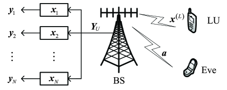
The procedure of the proposed RCT scheme is shown in Fig. 1. Different from conventional schemes where each user is only assigned with one PS, we simultaneously allocate N𝑁N (N>1𝑁1N>1) orthogonal PSs to the LU 111In this paper, we focus on a single-cell system with only one BS. In multi-cell environments, the PSs will be multiplexed in more than one cell, and the pilot contamination from other cells makes the problem mathematically much more complicated. We leave the multi-cell environments for future research.. Denote the set of PSs allocated to the LU as Φ{𝒙n}n=1NΦsuperscriptsubscriptsubscript𝒙𝑛𝑛1𝑁\Phi\triangleq\{\bm{x}_{n}\}_{n=1}^{N}, then we have 𝒙iH𝒙j=τ𝕀{i=j}superscriptsubscript𝒙𝑖𝐻subscript𝒙𝑗𝜏subscript𝕀𝑖𝑗\bm{x}_{i}^{H}\bm{x}_{j}=\tau\mathbb{I}_{\{i=j\}}, where τ𝜏\tau is the length of the PS. During the UCTP, the LU randomly chooses a PS from ΦΦ\Phi, denoted by 𝒙(L)superscript𝒙𝐿\bm{x}^{(L)}, to perform the uplink channel training. We emphasize that only the LU knows 𝒙(L)superscript𝒙𝐿\bm{x}^{(L)}. Both Eve and the BS know the set ΦΦ\Phi 222ΦΦ\Phi is assigned by the BS and shared between the BS and the LU, which is possible to be successfully intercepted by Eve. As the worst case, we assume that Eve perfectly knows ΦΦ\Phi. but do not know which PS is 𝒙(L)superscript𝒙𝐿\bm{x}^{(L)}. For a given instance of UCTP, the BS receives

𝒀UpL𝒉L(𝒙(L))H+pE𝒉E𝒂H+𝑽,subscript𝒀𝑈subscript𝑝𝐿subscript𝒉𝐿superscriptsuperscript𝒙𝐿𝐻subscript𝑝𝐸subscript𝒉𝐸superscript𝒂𝐻𝑽\displaystyle\bm{Y}_{U}\triangleq\sqrt{p_{L}}\bm{h}_{L}\left(\bm{x}^{(L)}\right)^{H}+\sqrt{p_{E}}\bm{h}_{E}\bm{a}^{H}+\bm{V}, (1)

where pLsubscript𝑝𝐿p_{L} and pEsubscript𝑝𝐸p_{E} are the powers of the LU and Eve, 𝒉LM×1(𝟎,𝑹L)subscript𝒉𝐿superscript𝑀1similar-to0subscript𝑹𝐿\bm{h}_{L}\in\mathbb{C}^{M\times 1}\sim\mathbb{CN}\left(\bm{0},\bm{R}_{L}\right) and 𝒉EM×1(𝟎,𝑹E)subscript𝒉𝐸superscript𝑀1similar-to0subscript𝑹𝐸\bm{h}_{E}\in\mathbb{C}^{M\times 1}\sim\mathbb{CN}\left(\bm{0},\bm{R}_{E}\right) denote the instantaneous channels of the LU and Eve, 𝒂τ×1𝒂superscript𝜏1\bm{a}\in\mathbb{C}^{\tau\times 1} is the attacking signal sequence transmitted by Eve, which will be detailed later on, and 𝑽M×τ𝑽superscript𝑀𝜏\bm{V}\in\mathbb{C}^{M\times\tau} is the noise with each element distributed as (0,σT2)0superscriptsubscript𝜎𝑇2\mathbb{CN}\left(0,\sigma_{T}^{2}\right). Due to the fact that 𝑹Lsubscript𝑹𝐿\bm{R}_{L} and 𝑹Esubscript𝑹𝐸\bm{R}_{E} change much slower than the instantaneous channels, we assume that the BS can obtain 𝑹Lsubscript𝑹𝐿\bm{R}_{L} and 𝑹Esubscript𝑹𝐸\bm{R}_{E} in advance333Note that if Tr(𝑹L𝑹E)=0Trsubscript𝑹𝐿subscript𝑹𝐸0\mathrm{Tr}\left(\bm{R}_{L}\bm{R}_{E}\right)=0, then the attack causes no impact on estimating LU’s channel, and in this paper, we only consider the cases where Tr(𝑹L𝑹E)0much-greater-thanTrsubscript𝑹𝐿subscript𝑹𝐸0\mathrm{Tr}\left(\bm{R}_{L}\bm{R}_{E}\right)\gg 0, which means that the attacks cause serious impact on the channel estimation procedure.. Note that similar assumptions has also been adopted in [29]. After receiving 𝒀Usubscript𝒀𝑈\bm{Y}_{U}, the BS matches 𝒀Usubscript𝒀𝑈\bm{Y}_{U} with the N𝑁N different orthogonal PSs in ΦΦ\Phi as illustrated in Fig. 1, and obtains N𝑁N channel observations, i.e.,

𝒚nsubscript𝒚𝑛\displaystyle\bm{y}_{n} φ𝒀U𝒙nabsent𝜑subscript𝒀𝑈subscript𝒙𝑛\displaystyle\triangleq\varphi\bm{Y}_{U}\bm{x}_{n}
=𝕀{𝒙n=𝒙(L)}𝒉L+φpE𝒉E𝒂H𝒙n+𝒛n,absentsubscript𝕀subscript𝒙𝑛superscript𝒙𝐿subscript𝒉𝐿𝜑subscript𝑝𝐸subscript𝒉𝐸superscript𝒂𝐻subscript𝒙𝑛subscript𝒛𝑛\displaystyle=\mathbb{I}_{\left\{\bm{x}_{n}=\bm{x}^{(L)}\right\}}\bm{h}_{L}+\varphi\sqrt{p_{E}}\bm{h}_{E}\bm{a}^{H}\bm{x}_{n}+\bm{z}_{n}, (2)

where 1nN1𝑛𝑁1\leq n\leq N, φ1τpL𝜑1𝜏subscript𝑝𝐿\varphi\triangleq\frac{1}{\tau\sqrt{p_{L}}}, and 𝒛nφ𝑽𝒙n(𝟎,σz2𝑰M)subscript𝒛𝑛𝜑𝑽subscript𝒙𝑛similar-to0superscriptsubscript𝜎𝑧2subscript𝑰𝑀\bm{z}_{n}\triangleq\varphi\bm{V}\bm{x}_{n}\sim\mathbb{CN}\left(\bm{0},\sigma_{z}^{2}\bm{I}_{M}\right) with σz2σT2τpLsuperscriptsubscript𝜎𝑧2superscriptsubscript𝜎𝑇2𝜏subscript𝑝𝐿\sigma_{z}^{2}\triangleq\frac{\sigma_{T}^{2}}{\tau p_{L}} is the equivalent Gaussian noise. Note that for nm𝑛𝑚n\neq m, 𝒛nsubscript𝒛𝑛\bm{z}_{n} and 𝒛msubscript𝒛𝑚\bm{z}_{m} are mutually independent because 𝒙nsubscript𝒙𝑛\bm{x}_{n} is orthogonal to 𝒙msubscript𝒙𝑚\bm{x}_{m}. Once obtaining the set of channel observations, i.e., Ψ{𝒚1,𝒚2,,𝒚N}Ψsubscript𝒚1subscript𝒚2subscript𝒚𝑁\Psi\triangleq\{\bm{y}_{1},\bm{y}_{2},\cdots,\bm{y}_{N}\}, the BS needs to figure out which PS is 𝒙(L)superscript𝒙𝐿\bm{x}^{(L)} in order to estimate LU’s channel, i.e, 𝒉Lsubscript𝒉𝐿\bm{h}_{L}. Before presenting the details, we first discuss the attacking schemes of Eve in the following.
Refer to caption
Figure 1: Uplink Training Model.

II-B Attacking Schemes of Eve

In the RCT scheme described above, Eve is incapable of always transmitting the same PS as that transmitted by the LU due to the randomness. We consider the following two possible attacking strategies of an active Eve,

  • Pilot spoofing attack (PSA): Eve randomly selects several PSs from ΦΦ\Phi and transmits a combination of them during the UCTP. Conventional PSA where Eve transmits the same PS as the LU [16] can be viewed as a special case of the PSA defined here;

  • Pilot jamming attack (PJA): Eve transmits randomly generated Gaussian interference to degrade the accuracy of the channel estimation.

We discuss the results of these two kinds of attack in the following.

II-B1 PSA during UCTP

Denote ΦEΦsubscriptΦ𝐸Φ\Phi_{E}\subseteq\Phi as the set of PSs selected by Eve during the UCTP. Then, the attacking signal sequence transmitted by Eve is

𝒂PSAn=1N𝕀{𝒙nΦE}ejωnχn𝒙n,subscript𝒂PSAsuperscriptsubscript𝑛1𝑁subscript𝕀subscript𝒙𝑛subscriptΦ𝐸superscriptejsubscript𝜔𝑛subscript𝜒𝑛subscript𝒙𝑛\displaystyle\bm{a}_{\mathrm{PSA}}\triangleq\sum_{n=1}^{N}\mathbb{I}_{\left\{\bm{x}_{n}\in\Phi_{E}\right\}}\mathrm{e}^{\mathrm{j}\omega_{n}}\sqrt{\chi_{n}}\bm{x}_{n}, (3)

where χnsubscript𝜒𝑛\chi_{n}, satisfying n=1N𝕀{𝒙nΦE}χn=1superscriptsubscript𝑛1𝑁subscript𝕀subscript𝒙𝑛subscriptΦ𝐸subscript𝜒𝑛1\sum_{n=1}^{N}\mathbb{I}_{\left\{\bm{x}_{n}\in\Phi_{E}\right\}}\chi_{n}=1, is the power factor for transmitting 𝒙nsubscript𝒙𝑛\boldsymbol{x}_{n}, ωnsubscript𝜔𝑛\omega_{n} is a random phase shift when transmitting 𝒙nsubscript𝒙𝑛\bm{x}_{n} which is unknown by the BS. We will show that an extra random phase shift, i.e., ejωnsuperscriptejsubscript𝜔𝑛\mathrm{e}^{\mathrm{j}\omega_{n}}, is necessary for Eve in Section III-C. In this paper, we assume that Eve uniformly allocate its power among different PSs, i.e., χn=1Ksubscript𝜒𝑛1𝐾\chi_{n}=\frac{1}{K} for 𝒙nΦEfor-allsubscript𝒙𝑛subscriptΦ𝐸\forall\bm{x}_{n}\in\Phi_{E} where K|ΦE|𝐾subscriptΦ𝐸K\triangleq\left|\Phi_{E}\right|. This is because Eve does not have any prior knowledge on which PS will be transmitted by the LU, and hence each PS does not have any priority to gain more power than the others. According to (3), 𝒚nsubscript𝒚𝑛\bm{y}_{n} in (2) becomes

𝒚n=𝕀{𝒙n=𝒙(L)}𝒉L+𝕀{𝒙nΦE}ejωnβPSA(K)𝒉E+𝒛n,subscript𝒚𝑛subscript𝕀subscript𝒙𝑛superscript𝒙𝐿subscript𝒉𝐿subscript𝕀subscript𝒙𝑛subscriptΦ𝐸superscriptejsubscript𝜔𝑛superscriptsubscript𝛽PSA𝐾subscript𝒉𝐸subscript𝒛𝑛\displaystyle\bm{y}_{n}=\mathbb{I}_{\{\bm{x}_{n}=\bm{x}^{(L)}\}}\bm{h}_{L}+\mathbb{I}_{\{\bm{x}_{n}\in\Phi_{E}\}}\mathrm{e}^{\mathrm{j}\omega_{n}}\beta_{\mathrm{PSA}}^{(K)}\bm{h}_{E}+\bm{z}_{n}, (4)

where βPSA(K)pEKpLsuperscriptsubscript𝛽PSA𝐾subscript𝑝𝐸𝐾subscript𝑝𝐿\beta_{\mathrm{PSA}}^{(K)}\triangleq\sqrt{\frac{p_{E}}{Kp_{L}}}. For notational simplicity, define two non-overlapping subsets of ΦΦ\Phi as

Φ¯PSA(E)superscriptsubscript¯ΦPSA𝐸\displaystyle\bar{\Phi}_{\mathrm{PSA}}^{(E)} {𝒙n|𝒙nΦE,𝒙n𝒙(L)}absentconditional-setsubscript𝒙𝑛formulae-sequencesubscript𝒙𝑛subscriptΦ𝐸subscript𝒙𝑛superscript𝒙𝐿\displaystyle\triangleq\left\{\bm{x}_{n}|\bm{x}_{n}\in\Phi_{E},\bm{x}_{n}\neq\bm{x}^{(L)}\right\}
={𝒙1(E),𝒙2(E),,𝒙QE(E)},absentsuperscriptsubscript𝒙1𝐸superscriptsubscript𝒙2𝐸superscriptsubscript𝒙subscript𝑄𝐸𝐸\displaystyle=\left\{\bm{x}_{1}^{(E)},\bm{x}_{2}^{(E)},\cdots,\bm{x}_{Q_{E}}^{(E)}\right\}, (5)
Φ¯PSA(F)superscriptsubscript¯ΦPSA𝐹\displaystyle\bar{\Phi}_{\mathrm{PSA}}^{(F)} Φ(Φ¯PSA(E){𝒙(L)})absentΦsuperscriptsubscript¯ΦPSA𝐸superscript𝒙𝐿\displaystyle\triangleq\Phi\setminus\left(\bar{\Phi}_{\mathrm{PSA}}^{(E)}\cup\{\bm{x}^{(L)}\}\right)
={𝒙1(F),𝒙2(F),,𝒙QF(F)},absentsuperscriptsubscript𝒙1𝐹superscriptsubscript𝒙2𝐹superscriptsubscript𝒙subscript𝑄𝐹𝐹\displaystyle=\left\{\bm{x}_{1}^{(F)},\bm{x}_{2}^{(F)},\cdots,\bm{x}_{Q_{F}}^{(F)}\right\}, (6)

where QE|Φ¯PSA(E)|subscript𝑄𝐸superscriptsubscript¯ΦPSA𝐸Q_{E}\triangleq|\bar{\Phi}_{\mathrm{PSA}}^{(E)}| and QF|Φ¯PSA(F)|subscript𝑄𝐹superscriptsubscript¯ΦPSA𝐹Q_{F}\triangleq|\bar{\Phi}_{\mathrm{PSA}}^{(F)}|. Based on (II-B1) and (II-B1), we can rewrite 𝒚nsubscript𝒚𝑛\bm{y}_{n} in (4) as,

𝒚nsubscript𝒚𝑛\displaystyle\bm{y}_{n} ={𝒚(L),𝒙n=𝒙(L),𝒚i(E),𝒙n=𝒙i(E)Φ¯PSA(E),𝒚i(F),𝒙n=𝒙i(F)Φ¯PSA(F),\displaystyle=\left\{\begin{aligned} \bm{y}^{(L)},&\quad\quad\bm{x}_{n}=\bm{x}^{(L)},\\ \bm{y}_{i}^{(E)},&\quad\quad\bm{x}_{n}=\bm{x}_{i}^{(E)}\in\bar{\Phi}_{\mathrm{PSA}}^{(E)},\\ \bm{y}_{i}^{(F)},&\quad\quad\bm{x}_{n}=\bm{x}_{i}^{(F)}\in\bar{\Phi}_{\mathrm{PSA}}^{(F)},\end{aligned}\right. (7)
𝒚(L)superscript𝒚𝐿\displaystyle\bm{y}^{(L)} 𝒉L+𝕀{𝒙(L)ΦE}ejω(L)βPSA(K)𝒉E+𝒛(L),absentsubscript𝒉𝐿subscript𝕀superscript𝒙𝐿subscriptΦ𝐸superscriptejsuperscript𝜔𝐿superscriptsubscript𝛽PSA𝐾subscript𝒉𝐸superscript𝒛𝐿\displaystyle\triangleq\bm{h}_{L}+\mathbb{I}_{\{\bm{x}^{(L)}\in\Phi_{E}\}}\mathrm{e}^{\mathrm{j}\omega^{(L)}}\beta_{\mathrm{PSA}}^{(K)}\bm{h}_{E}+\bm{z}^{(L)},
𝒚i(E)superscriptsubscript𝒚𝑖𝐸\displaystyle\bm{y}_{i}^{(E)} ejωi(E)βPSA(K)𝒉E+𝒛i(E),absentsuperscriptejsuperscriptsubscript𝜔𝑖𝐸superscriptsubscript𝛽PSA𝐾subscript𝒉𝐸superscriptsubscript𝒛𝑖𝐸\displaystyle\triangleq\mathrm{e}^{\mathrm{j}\omega_{i}^{(E)}}\beta_{\mathrm{PSA}}^{(K)}\bm{h}_{E}+\bm{z}_{i}^{(E)},
𝒚i(F)superscriptsubscript𝒚𝑖𝐹\displaystyle\bm{y}_{i}^{(F)} 𝒛i(F),absentsuperscriptsubscript𝒛𝑖𝐹\displaystyle\triangleq\bm{z}_{i}^{(F)},

where 𝒛(L)n=1N𝒛n𝕀{𝒙n=𝒙(L)}superscript𝒛𝐿superscriptsubscript𝑛1𝑁subscript𝒛𝑛subscript𝕀subscript𝒙𝑛superscript𝒙𝐿\bm{z}^{(L)}\triangleq\sum_{n=1}^{N}\bm{z}_{n}\mathbb{I}_{\{\bm{x}_{n}=\bm{x}^{(L)}\}}, 𝒛i(E)n=1N𝒛n𝕀{𝒙n=𝒙i(E)}superscriptsubscript𝒛𝑖𝐸superscriptsubscript𝑛1𝑁subscript𝒛𝑛subscript𝕀subscript𝒙𝑛superscriptsubscript𝒙𝑖𝐸\bm{z}_{i}^{(E)}\triangleq\sum_{n=1}^{N}\bm{z}_{n}\mathbb{I}_{\{\bm{x}_{n}=\bm{x}_{i}^{(E)}\}}, 𝒛i(F)n=1N𝒛n𝕀{𝒙n=𝒙i(F)}superscriptsubscript𝒛𝑖𝐹superscriptsubscript𝑛1𝑁subscript𝒛𝑛subscript𝕀subscript𝒙𝑛superscriptsubscript𝒙𝑖𝐹\bm{z}_{i}^{(F)}\triangleq\sum_{n=1}^{N}\bm{z}_{n}\mathbb{I}_{\{\bm{x}_{n}=\bm{x}_{i}^{(F)}\}}, ω(L)n=1Nωn𝕀{𝒙n=𝒙(L)}superscript𝜔𝐿superscriptsubscript𝑛1𝑁subscript𝜔𝑛subscript𝕀subscript𝒙𝑛superscript𝒙𝐿\omega^{(L)}\triangleq\sum_{n=1}^{N}\omega_{n}\mathbb{I}_{\{\bm{x}_{n}=\bm{x}^{(L)}\}}, and ωi(E)n=1Nωn𝕀{𝒙n=𝒙i(E)}superscriptsubscript𝜔𝑖𝐸superscriptsubscript𝑛1𝑁subscript𝜔𝑛subscript𝕀subscript𝒙𝑛superscriptsubscript𝒙𝑖𝐸\omega_{i}^{(E)}\triangleq\sum_{n=1}^{N}\omega_{n}\mathbb{I}_{\{\bm{x}_{n}=\bm{x}_{i}^{(E)}\}}. According to (7), we can divide Ψ={𝒚n}n=1NΨsuperscriptsubscriptsubscript𝒚𝑛𝑛1𝑁\Psi=\{\bm{y}_{n}\}_{n=1}^{N} into three non-overlapping subsets, i.e., Ψ={𝒚(L)}ΨPSA(E)ΨPSA(F)Ψsuperscript𝒚𝐿superscriptsubscriptΨPSA𝐸superscriptsubscriptΨPSA𝐹\Psi=\left\{\bm{y}^{(L)}\right\}\cup\Psi_{\mathrm{PSA}}^{(E)}\cup\Psi_{\mathrm{PSA}}^{(F)}, where we have ΨPSA(E){𝒚1(E),,𝒚QE(E)}superscriptsubscriptΨPSA𝐸superscriptsubscript𝒚1𝐸superscriptsubscript𝒚subscript𝑄𝐸𝐸\Psi_{\mathrm{PSA}}^{(E)}\triangleq\left\{\bm{y}_{1}^{(E)},\cdots,\bm{y}_{Q_{E}}^{(E)}\right\} and ΨPSA(F){𝒚1(F),,𝒚QF(F)}superscriptsubscriptΨPSA𝐹superscriptsubscript𝒚1𝐹superscriptsubscript𝒚subscript𝑄𝐹𝐹\Psi_{\mathrm{PSA}}^{(F)}\triangleq\left\{\bm{y}_{1}^{(F)},\cdots,\bm{y}_{Q_{F}}^{(F)}\right\}.

We have to point out that the estimation of the legitimate channel is strongly affected by the realization of 𝒙(L)superscript𝒙𝐿\bm{x}^{(L)} and ΦEsubscriptΦ𝐸\Phi_{E}. Due to the fact that 𝒙(L)superscript𝒙𝐿\bm{x}^{(L)} and ΦEsubscriptΦ𝐸\Phi_{E} are independently and randomly selected by the LU and Eve, respectively, we refer to the occurrence of a hit event when 𝒙(L)ΦEsuperscript𝒙𝐿subscriptΦ𝐸\bm{x}^{(L)}\in\Phi_{E}, i.e., the PS transmitted by the LU is occasionally selected by Eve.

II-B2 PJA during UCTP

During the UCTP, Eve transmits Gaussian random jamming signals 𝒂PJA(𝟎,𝑰τ)similar-tosubscript𝒂PJA0subscript𝑰𝜏\bm{a}_{\mathrm{PJA}}\sim\mathbb{CN}\left(\bm{0},\bm{I}_{\tau}\right). Then, 𝒚nsubscript𝒚𝑛\bm{y}_{n} in (2) becomes

𝒚n=φ𝒀U𝒙n=𝕀{𝒙n=𝒙(L)}𝒉L+μnβPJA𝒉E+𝒛n,subscript𝒚𝑛𝜑subscript𝒀𝑈subscript𝒙𝑛subscript𝕀subscript𝒙𝑛superscript𝒙𝐿subscript𝒉𝐿subscript𝜇𝑛subscript𝛽PJAsubscript𝒉𝐸subscript𝒛𝑛\displaystyle\bm{y}_{n}=\varphi\bm{Y}_{U}\bm{x}_{n}=\mathbb{I}_{\left\{\bm{x}_{n}=\bm{x}^{(L)}\right\}}\bm{h}_{L}+\mu_{n}\beta_{\mathrm{PJA}}\bm{h}_{E}+\bm{z}_{n}, (8)

where we have μn1τ𝒂PJAH𝒙n(E)(0,1τ)subscript𝜇𝑛1𝜏superscriptsubscript𝒂PJA𝐻superscriptsubscript𝒙𝑛𝐸similar-to01𝜏\mu_{n}\triangleq\frac{1}{\tau}\bm{a}_{\mathrm{PJA}}^{H}\bm{x}_{n}^{(E)}\sim\mathbb{CN}\left(0,\frac{1}{\tau}\right) and βPJApEpLsubscript𝛽PJAsubscript𝑝𝐸subscript𝑝𝐿\beta_{\mathrm{PJA}}\triangleq\sqrt{\frac{p_{E}}{p_{L}}}. Define Φ¯PJA(E)superscriptsubscript¯ΦPJA𝐸\bar{\Phi}_{\mathrm{PJA}}^{(E)} as a subset of ΦΦ\Phi which is written as

Φ¯PJA(E)Φ{𝒙(L)}={𝒙ˇ1(E),,𝒙ˇN1(E)}.superscriptsubscript¯ΦPJA𝐸Φsuperscript𝒙𝐿superscriptsubscriptˇ𝒙1𝐸superscriptsubscriptˇ𝒙𝑁1𝐸\displaystyle\bar{\Phi}_{\mathrm{PJA}}^{(E)}\triangleq\Phi\setminus\{\bm{x}^{(L)}\}=\{\check{\bm{x}}_{1}^{(E)},\cdots,\check{\bm{x}}_{N-1}^{(E)}\}. (9)

Similar to (7), we rewrite the channel observations in (8) under PJA as

𝒚nsubscript𝒚𝑛\displaystyle\bm{y}_{n} ={𝒚(L),𝒙n=𝒙(L),𝒚i(E),𝒙n=𝒙ˇi(E)Φ¯PJA(E),\displaystyle=\left\{\begin{aligned} \bm{y}^{(L)},&\quad\quad\bm{x}_{n}=\bm{x}^{(L)},\\ \bm{y}_{i}^{(E)},&\quad\quad\bm{x}_{n}=\check{\bm{x}}_{i}^{(E)}\in\bar{\Phi}_{\mathrm{PJA}}^{(E)},\end{aligned}\right. (10)
𝒚(L)superscript𝒚𝐿\displaystyle\bm{y}^{(L)} 𝒉L+μ(L)βPJA𝒉E+𝒛(L),absentsubscript𝒉𝐿superscript𝜇𝐿subscript𝛽PJAsubscript𝒉𝐸superscript𝒛𝐿\displaystyle\triangleq\bm{h}_{L}+\mu^{(L)}\beta_{\mathrm{PJA}}\bm{h}_{E}+\bm{z}^{(L)},
𝒚i(E)superscriptsubscript𝒚𝑖𝐸\displaystyle\bm{y}_{i}^{(E)} μi(E)βPJA𝒉E+𝒛i(E),absentsuperscriptsubscript𝜇𝑖𝐸subscript𝛽PJAsubscript𝒉𝐸superscriptsubscript𝒛𝑖𝐸\displaystyle\triangleq\mu_{i}^{(E)}\beta_{\mathrm{PJA}}\bm{h}_{E}+\bm{z}_{i}^{(E)},

where we have 𝒛i(E)n=1N𝒛n𝕀{𝒙n=𝒙ˇi(E)}superscriptsubscript𝒛𝑖𝐸superscriptsubscript𝑛1𝑁subscript𝒛𝑛subscript𝕀subscript𝒙𝑛superscriptsubscriptˇ𝒙𝑖𝐸\bm{z}_{i}^{(E)}\triangleq\sum_{n=1}^{N}\bm{z}_{n}\mathbb{I}_{\{\bm{x}_{n}=\check{\bm{x}}_{i}^{(E)}\}}, μ(L)n=1Nμn𝕀{𝒙n=𝒙(L)}superscript𝜇𝐿superscriptsubscript𝑛1𝑁subscript𝜇𝑛subscript𝕀subscript𝒙𝑛superscript𝒙𝐿\mu^{(L)}\triangleq\sum_{n=1}^{N}\mu_{n}\mathbb{I}_{\{\bm{x}_{n}=\bm{x}^{(L)}\}}, and μi(E)n=1Nμn𝕀{𝒙n=𝒙ˇi(E)}superscriptsubscript𝜇𝑖𝐸superscriptsubscript𝑛1𝑁subscript𝜇𝑛subscript𝕀subscript𝒙𝑛superscriptsubscriptˇ𝒙𝑖𝐸\mu_{i}^{(E)}\triangleq\sum_{n=1}^{N}\mu_{n}\mathbb{I}_{\{\bm{x}_{n}=\check{\bm{x}}_{i}^{(E)}\}}. According to (10), we divide ΨΨ\Psi under PJA into two non-overlapping subsets, i.e., Ψ={𝒚(L)}ΨPJA(E)Ψsuperscript𝒚𝐿superscriptsubscriptΨPJA𝐸\Psi=\left\{\bm{y}^{(L)}\right\}\cup\Psi_{\mathrm{PJA}}^{(E)}, where we define ΨPJA(E){𝒚1(E),,𝒚N1(E)}superscriptsubscriptΨPJA𝐸superscriptsubscript𝒚1𝐸superscriptsubscript𝒚𝑁1𝐸\Psi_{\mathrm{PJA}}^{(E)}\triangleq\left\{\bm{y}_{1}^{(E)},\cdots,\bm{y}_{N-1}^{(E)}\right\}.

As we can see from (7) and (10), the BS obtains multiple channel observations, which contains both LU’s and Eve’s CSI. A critical step for the BS to achieve secrecy transmission is to figure out which channel observation is 𝒚(L)superscript𝒚𝐿\bm{y}^{(L)} so as to estimate the legitimate and illegitimate channels simultaneously. We will discuss the detailed steps for the BS to identify 𝒚(L)superscript𝒚𝐿\bm{y}^{(L)}, to estimate the channels, and to design the SB vector under the PSA, in Section III, Section IV, and Section V, respectively. Secure transmission under the PJA will be discussed in Section VI in a similar manner.

   Remark 1.

The proposed scheme can be easily extended to a multi-user system because we exploit the orthogonality among different PSs. More specifically, in a system with U𝑈U users, the set of PSs ΦΦ\Phi can be divided into U𝑈U non-overlapping subsets, i.e., Φ(1),Φ(2),,Φ(U)ΦsuperscriptΦ1superscriptΦ2superscriptΦ𝑈Φ\Phi^{(1)},\Phi^{(2)},\cdots,\Phi^{(U)}\subset\Phi, with Φ(u)superscriptΦ𝑢\Phi^{(u)} allocated to the uthsuperscript𝑢thu^{\mathrm{th}} user, and all the following discussions hold as well. In following part of this paper, unless specified, we always assume that there is only one user and all the PSs are allocated to the user, i.e., N=τ𝑁𝜏N=\tau.

III Determining the PS of LU under PSA

In this section, we present the method for the BS to determine which PS is 𝒙(L)superscript𝒙𝐿\bm{x}^{(L)}, or equivalently speaking, which channel observation is 𝒚(L)superscript𝒚𝐿\bm{y}^{(L)}, under the PSA. We also evaluate the detection performance in terms of the EDR, i.e., the probability that the BS makes an incorrect decision on 𝒚(L)superscript𝒚𝐿\bm{y}^{(L)}.

We have to point out that, as shown in (7), channel observations in ΨPSA(F)superscriptsubscriptΨPSA𝐹\Psi_{\mathrm{PSA}}^{(F)} contains neither LU’s nor Eve’s CSI, and therefore, as a pre-processing step, the BS needs to distinguish ΨPSA(C){𝒚(L)}ΨPSA(E)superscriptsubscriptΨPSA𝐶superscript𝒚𝐿superscriptsubscriptΨPSA𝐸\Psi_{\mathrm{PSA}}^{(C)}\triangleq\left\{\bm{y}^{(L)}\right\}\cup\Psi_{\mathrm{PSA}}^{(E)} from ΨPSA(F)superscriptsubscriptΨPSA𝐹\Psi_{\mathrm{PSA}}^{(F)}. To realize this, the BS can simply classify 𝒚nsubscript𝒚𝑛\bm{y}_{n}, (1nN1𝑛𝑁1\leq n\leq N), into ΨPSA(C)superscriptsubscriptΨPSA𝐶\Psi_{\mathrm{PSA}}^{(C)} or ΨPSA(F)superscriptsubscriptΨPSA𝐹\Psi_{\mathrm{PSA}}^{(F)} by comparing their powers with a predesigned threshold ΛCsubscriptΛ𝐶\Lambda_{C}, i.e.,𝒚n2ΨPSA(F)ΨPSA(C)ΛCsuperscriptsubscriptgreater-than-or-equals-or-less-thansuperscriptsubscriptΨPSA𝐹superscriptsubscriptΨPSA𝐶superscriptnormsubscript𝒚𝑛2subscriptΛ𝐶\left\|\bm{y}_{n}\right\|^{2}\gtreqless_{\Psi_{\mathrm{PSA}}^{(F)}}^{\Psi_{\mathrm{PSA}}^{(C)}}\Lambda_{C}. We observe that the powers of 𝒚(L)superscript𝒚𝐿\bm{y}^{(L)} and 𝒚n(E)superscriptsubscript𝒚𝑛𝐸\bm{y}_{n}^{(E)} are much larger than 𝒚n(F)superscriptsubscript𝒚𝑛𝐹\bm{y}_{n}^{(F)} due to the fact that the noise floor of 𝒛n(F)superscriptsubscript𝒛𝑛𝐹\bm{z}_{n}^{(F)} is generally small, especially when pLsubscript𝑝𝐿p_{L} and τ𝜏\tau are large. Therefore, we make a reasonable assumption that the BS has already obtained the effective channel observation set ΨPSA(C)superscriptsubscriptΨPSA𝐶\Psi_{\mathrm{PSA}}^{(C)} correctly. For notational simplicity, we define QCsubscript𝑄𝐶Q_{C} as the cardinality of ΨPSA(C)superscriptsubscriptΨPSA𝐶\Psi_{\mathrm{PSA}}^{(C)}, i.e., QC|ΨPSA(C)|subscript𝑄𝐶superscriptsubscriptΨPSA𝐶Q_{C}\triangleq|\Psi_{\mathrm{PSA}}^{(C)}|.

Now, we provide our method for the BS to determine which channel observation in ΨPSA(C)superscriptsubscriptΨPSA𝐶\Psi_{\mathrm{PSA}}^{(C)} is 𝒚(L)superscript𝒚𝐿\bm{y}^{(L)}. We note that, the detection is highly related to the parameter K𝐾K, which is, however, chosen by Eve and unknown by the BS. For simplicity, In the first step we discuss the cases where K𝐾K is known by BS, and classify our discussions according to the value of K𝐾K and whether or not a hit event occurs. After that, we extend our method to handle the cases when K𝐾K is unknown.

III-A K=1𝐾1K=1 and Eve successfully hits LU’s PS

In this cases, undoubtedly, we have ΨPSA(C)={𝒚(L)}superscriptsubscriptΨPSA𝐶superscript𝒚𝐿\Psi_{\mathrm{PSA}}^{(C)}=\left\{\bm{y}^{(L)}\right\} where 𝒚(L)=𝒉L+ejω(L)βPSA(1)𝒉E+𝒛(L)superscript𝒚𝐿subscript𝒉𝐿superscriptejsuperscript𝜔𝐿superscriptsubscript𝛽PSA1subscript𝒉𝐸superscript𝒛𝐿\bm{y}^{(L)}=\bm{h}_{L}+\mathrm{e}^{\mathrm{j}\omega^{(L)}}\beta_{\mathrm{PSA}}^{(1)}\bm{h}_{E}+\bm{z}^{(L)}. We note that this is the case of the conventional PSA and has been discussed in [25, 24, 23, 27, 28, 29, 26].

III-B K=1𝐾1K=1 and Eve fails to hit LU’s PS

In this case, we have QC=2subscript𝑄𝐶2Q_{C}=2. Without loss of generality, denote ΨPSA(C)={𝒚1,𝒚2}superscriptsubscriptΨPSA𝐶subscript𝒚1subscript𝒚2\Psi_{\mathrm{PSA}}^{(C)}=\left\{\bm{y}_{1},\bm{y}_{2}\right\}. To determine which one of 𝒚1subscript𝒚1\bm{y}_{1} and 𝒚2subscript𝒚2\bm{y}_{2} is 𝒚(L)superscript𝒚𝐿\bm{y}^{(L)}, we formulate a hypothesis test problem, i.e.,

[𝒚1𝒚2]={[𝒚(L)𝒚(E)]=[𝒉L+𝒛(L)ejω(E)βPSA(1)𝒉E+𝒛(E)],0(1,2),[𝒚(E)𝒚(L)]=[ejω(E)βPSA(1)𝒉E+𝒛(E)𝒉L+𝒛(L)],1(1,2),\displaystyle\begin{bmatrix}\bm{y}_{1}\\ \bm{y}_{2}\\ \end{bmatrix}=\left\{\begin{aligned} \begin{bmatrix}\bm{y}^{(L)}\\ \bm{y}^{(E)}\\ \end{bmatrix}=\begin{bmatrix}\bm{h}_{L}+\bm{z}^{(L)}\\ \mathrm{e}^{\mathrm{j}\omega^{(E)}}\beta_{\mathrm{PSA}}^{(1)}\bm{h}_{E}+\bm{z}^{(E)}\\ \end{bmatrix},\mathcal{H}_{0}^{(1,2)},\\ \begin{bmatrix}\bm{y}^{(E)}\\ \bm{y}^{(L)}\\ \end{bmatrix}=\begin{bmatrix}\mathrm{e}^{\mathrm{j}\omega^{(E)}}\beta_{\mathrm{PSA}}^{(1)}\bm{h}_{E}+\bm{z}^{(E)}\\ \bm{h}_{L}+\bm{z}^{(L)}\\ \end{bmatrix},\mathcal{H}_{1}^{(1,2)},\end{aligned}\right. (11)

where 0(1,2)superscriptsubscript012\mathcal{H}_{0}^{(1,2)} represents that 𝒚1=𝒚(L)subscript𝒚1superscript𝒚𝐿\bm{y}_{1}=\bm{y}^{(L)} and 1(1,2)superscriptsubscript112\mathcal{H}_{1}^{(1,2)} represents that 𝒚2=𝒚(L)subscript𝒚2superscript𝒚𝐿\bm{y}_{2}=\bm{y}^{(L)}. To determine 𝒚(L)superscript𝒚𝐿\bm{y}^{(L)}, the logarithmic likelihood ratio (LLR) test is written as

T1(2)lnp(𝒈|0(1,2))lnp(𝒈|1(1,2))1(1,2)0(1,2)0,superscriptsubscript𝑇12𝑝conditional𝒈superscriptsubscript012𝑝conditional𝒈superscriptsubscript112superscriptsubscriptgreater-than-or-equals-or-less-thansuperscriptsubscript112superscriptsubscript0120\displaystyle T_{1}^{(2)}\triangleq\ln p\left(\bm{g}|\mathcal{H}_{0}^{(1,2)}\right)-\ln p\left(\bm{g}|\mathcal{H}_{1}^{(1,2)}\right){\gtreqless}_{\mathcal{H}_{1}^{(1,2)}}^{\mathcal{H}_{0}^{(1,2)}}0, (12)

where 𝒈[𝒚1H,𝒚2H]H𝒈superscriptsuperscriptsubscript𝒚1𝐻superscriptsubscript𝒚2𝐻𝐻\bm{g}\triangleq\left[\bm{y}_{1}^{H},\bm{y}_{2}^{H}\right]^{H}, p(𝒈|0(1,2))𝑝conditional𝒈superscriptsubscript012p\left(\bm{g}|\mathcal{H}_{0}^{(1,2)}\right) and p(𝒈|1(1,2))𝑝conditional𝒈superscriptsubscript112p\left(\bm{g}|\mathcal{H}_{1}^{(1,2)}\right) are the PDFs of 𝒈𝒈\bm{g} conditioned on 0(1,2)superscriptsubscript012\mathcal{H}_{0}^{(1,2)} and 1(1,2)superscriptsubscript112\mathcal{H}_{1}^{(1,2)}, respectively. Note that if 0(1,2)superscriptsubscript012\mathcal{H}_{0}^{(1,2)} is true, 𝒚1subscript𝒚1\bm{y}_{1} and 𝒚2subscript𝒚2\bm{y}_{2} are independently distributed as (𝟎,𝑹L,z)0subscript𝑹𝐿𝑧\mathbb{CN}\left(\bm{0},\bm{R}_{L,z}\right) and (𝟎,𝑹E,z(1))0superscriptsubscript𝑹𝐸𝑧1\mathbb{CN}\left(\bm{0},\bm{R}_{E,z}^{(1)}\right), respectively, and if 1(1,2)superscriptsubscript112\mathcal{H}_{1}^{(1,2)} is true, 𝒚1subscript𝒚1\bm{y}_{1} and 𝒚2subscript𝒚2\bm{y}_{2} are independently distributed as (𝟎,𝑹E,z(1))0superscriptsubscript𝑹𝐸𝑧1\mathbb{CN}\left(\bm{0},\bm{R}_{E,z}^{(1)}\right) and (𝟎,𝑹L,z)0subscript𝑹𝐿𝑧\mathbb{CN}\left(\bm{0},\bm{R}_{L,z}\right), respectively, where we have 𝑹L,z𝑹L+σz2𝑰subscript𝑹𝐿𝑧subscript𝑹𝐿superscriptsubscript𝜎𝑧2𝑰\bm{R}_{L,z}\triangleq\bm{R}_{L}+\sigma_{z}^{2}\bm{I} and 𝑹E,z(1)|βPSA(1)|2𝑹E+σz2𝑰superscriptsubscript𝑹𝐸𝑧1superscriptsuperscriptsubscript𝛽PSA12subscript𝑹𝐸superscriptsubscript𝜎𝑧2𝑰\bm{R}_{E,z}^{(1)}\triangleq|\beta_{\mathrm{PSA}}^{(1)}|^{2}\bm{R}_{E}+\sigma_{z}^{2}\bm{I}. Therefore, (12) can be further simplified as

T1(2)superscriptsubscript𝑇12\displaystyle T_{1}^{(2)} =𝒚1H((𝑹E,z(1))1𝑹L,z1)𝒚1absentsuperscriptsubscript𝒚1𝐻superscriptsuperscriptsubscript𝑹𝐸𝑧11superscriptsubscript𝑹𝐿𝑧1subscript𝒚1\displaystyle=\bm{y}_{1}^{H}\left(\left(\bm{R}_{E,z}^{(1)}\right)^{-1}-\bm{R}_{L,z}^{-1}\right)\bm{y}_{1}
+𝒚2H(𝑹L,z1(𝑹E,z(1))1)𝒚21(1,2)0(1,2)0.superscriptsubscriptgreater-than-or-equals-or-less-thansuperscriptsubscript112superscriptsubscript012superscriptsubscript𝒚2𝐻superscriptsubscript𝑹𝐿𝑧1superscriptsuperscriptsubscript𝑹𝐸𝑧11subscript𝒚20\displaystyle\quad+\bm{y}_{2}^{H}\left(\bm{R}_{L,z}^{-1}-\left(\bm{R}_{E,z}^{(1)}\right)^{-1}\right)\bm{y}_{2}{\gtreqless}_{\mathcal{H}_{1}^{(1,2)}}^{\mathcal{H}_{0}^{(1,2)}}0. (13)

According to (13), the EDR in this case is given by

𝒫EDR(1,2)superscriptsubscript𝒫EDR12\displaystyle\mathcal{P}_{\mathrm{EDR}}^{(1,2)} 𝒫{T1(2)<0|0(1,2)}absent𝒫superscriptsubscript𝑇12bra0superscriptsubscript012\displaystyle\triangleq\mathcal{P}\left\{T_{1}^{(2)}<0|\mathcal{H}_{0}^{(1,2)}\right\}
=𝒫{T1(2)>0|1(1,2)}.absent𝒫conditional-setsuperscriptsubscript𝑇120superscriptsubscript112\displaystyle=\mathcal{P}\left\{T_{1}^{(2)}>0|\mathcal{H}_{1}^{(1,2)}\right\}. (14)

The calculation of 𝒫EDR(1,2)superscriptsubscript𝒫EDR12\mathcal{P}_{\mathrm{EDR}}^{(1,2)} is provided in the following theorem.

   Theorem 1.

𝒫EDR(1,2)superscriptsubscript𝒫EDR12\mathcal{P}_{\mathrm{EDR}}^{(1,2)} can be calculated as

𝒫EDR(1,2)superscriptsubscript𝒫EDR12\displaystyle\mathcal{P}_{\mathrm{EDR}}^{(1,2)} =𝒫{𝒘H𝚵𝒘<0},absent𝒫superscript𝒘𝐻𝚵𝒘0\displaystyle=\mathcal{P}\left\{\bm{w}^{H}\bm{\Xi}\bm{w}<0\right\}, (15)

where 𝒘𝒘\bm{w} is a Gaussian random vector distributed as (𝟎,𝑰2M)0subscript𝑰2𝑀\mathbb{CN}\left(\bm{0},\bm{I}_{2M}\right), and

𝚵𝚵\displaystyle\bm{\Xi} [𝚵1𝑰M,𝟎M×M𝟎M×M,𝚵2𝑰M],absentmatrixsubscript𝚵1subscript𝑰𝑀subscript0𝑀𝑀subscript0𝑀𝑀subscript𝚵2subscript𝑰𝑀\displaystyle\triangleq\begin{bmatrix}\bm{\Xi}_{1}-\bm{I}_{M},&\bm{0}_{M\times M}\\ \bm{0}_{M\times M},&\bm{\Xi}_{2}-\bm{I}_{M}\\ \end{bmatrix}, (16)

with 𝚵1𝑹L,z12(𝑹E,z(1))1𝑹L,z12subscript𝚵1superscriptsubscript𝑹𝐿𝑧12superscriptsuperscriptsubscript𝑹𝐸𝑧11superscriptsubscript𝑹𝐿𝑧12\bm{\Xi}_{1}\triangleq\bm{R}_{L,z}^{\frac{1}{2}}\left(\bm{R}_{E,z}^{(1)}\right)^{-1}\bm{R}_{L,z}^{\frac{1}{2}} and 𝚵2(𝑹E,z(1))12𝑹L,z1(𝑹E,z(1))12subscript𝚵2superscriptsuperscriptsubscript𝑹𝐸𝑧112superscriptsubscript𝑹𝐿𝑧1superscriptsuperscriptsubscript𝑹𝐸𝑧112\bm{\Xi}_{2}\triangleq\left(\bm{R}_{E,z}^{(1)}\right)^{\frac{1}{2}}\bm{R}_{L,z}^{-1}\left(\bm{R}_{E,z}^{(1)}\right)^{\frac{1}{2}}.

Proof:

The detailed derivation of (16) is provided in (17) at the top of the next page,

𝒫EDR(1,2)superscriptsubscript𝒫EDR12\displaystyle\mathcal{P}_{\mathrm{EDR}}^{(1,2)} =𝒫{𝒚1H((𝑹E,z(1))1𝑹L,z1)𝒚1+𝒚2H(𝑹L,z1(𝑹E,z(1))1)𝒚2<0|0(1,2)}absent𝒫superscriptsubscript𝒚1𝐻superscriptsuperscriptsubscript𝑹𝐸𝑧11superscriptsubscript𝑹𝐿𝑧1subscript𝒚1superscriptsubscript𝒚2𝐻superscriptsubscript𝑹𝐿𝑧1superscriptsuperscriptsubscript𝑹𝐸𝑧11subscript𝒚2bra0superscriptsubscript012\displaystyle=\mathcal{P}\left\{\bm{y}_{1}^{H}\left(\left(\bm{R}_{E,z}^{(1)}\right)^{-1}-\bm{R}_{L,z}^{-1}\right)\bm{y}_{1}+\bm{y}_{2}^{H}\left(\bm{R}_{L,z}^{-1}-\left(\bm{R}_{E,z}^{(1)}\right)^{-1}\right)\bm{y}_{2}<0|\mathcal{H}_{0}^{(1,2)}\right\}
=𝒫{𝒚1H𝑹L,z12(𝚵1𝑰M)𝑹L,z12𝒚1+𝒚2H(𝑹E,z(1))12(𝚵2𝑰M)(𝑹E,z(1))12𝒚2<0|0(1,2)}absent𝒫superscriptsubscript𝒚1𝐻superscriptsubscript𝑹𝐿𝑧12subscript𝚵1subscript𝑰𝑀superscriptsubscript𝑹𝐿𝑧12subscript𝒚1superscriptsubscript𝒚2𝐻superscriptsuperscriptsubscript𝑹𝐸𝑧112subscript𝚵2subscript𝑰𝑀superscriptsuperscriptsubscript𝑹𝐸𝑧112subscript𝒚2bra0superscriptsubscript012\displaystyle=\mathcal{P}\left\{\bm{y}_{1}^{H}\bm{R}_{L,z}^{-\frac{1}{2}}\left(\bm{\Xi}_{1}-\bm{I}_{M}\right)\bm{R}_{L,z}^{-\frac{1}{2}}\bm{y}_{1}+\bm{y}_{2}^{H}\left(\bm{R}_{E,z}^{(1)}\right)^{-\frac{1}{2}}\left(\bm{\Xi}_{2}-\bm{I}_{M}\right)\left(\bm{R}_{E,z}^{(1)}\right)^{-\frac{1}{2}}\bm{y}_{2}<0|\mathcal{H}_{0}^{(1,2)}\right\}
=𝒫{𝒘1H(𝚵1𝑰M)𝒘1+𝒘2(𝚵2𝑰M)𝒘2H<0}=𝒫{𝒘H𝚵𝒘<0}.absent𝒫superscriptsubscript𝒘1𝐻subscript𝚵1subscript𝑰𝑀subscript𝒘1subscript𝒘2subscript𝚵2subscript𝑰𝑀superscriptsubscript𝒘2𝐻0𝒫superscript𝒘𝐻𝚵𝒘0\displaystyle=\mathcal{P}\left\{\bm{w}_{1}^{H}\left(\bm{\Xi}_{1}-\bm{I}_{M}\right)\bm{w}_{1}+\bm{w}_{2}\left(\bm{\Xi}_{2}-\bm{I}_{M}\right)\bm{w}_{2}^{H}<0\right\}=\mathcal{P}\left\{\bm{w}^{H}\bm{\Xi}\bm{w}<0\right\}. (17)

where we have 𝒘1𝑹L,z12𝒚1subscript𝒘1superscriptsubscript𝑹𝐿𝑧12subscript𝒚1\bm{w}_{1}\triangleq\bm{R}_{L,z}^{-\frac{1}{2}}\bm{y}_{1}, 𝒘2(𝑹E,z(1))12𝒚2subscript𝒘2superscriptsuperscriptsubscript𝑹𝐸𝑧112subscript𝒚2\bm{w}_{2}\triangleq\left(\bm{R}_{E,z}^{(1)}\right)^{-\frac{1}{2}}\bm{y}_{2}, 𝒘[𝒘1H,𝒘2H]H𝒘superscriptsuperscriptsubscript𝒘1𝐻superscriptsubscript𝒘2𝐻𝐻\bm{w}\triangleq\left[\bm{w}_{1}^{H},\bm{w}_{2}^{H}\right]^{H}, and 𝚵1subscript𝚵1\bm{\Xi}_{1}, 𝚵2subscript𝚵2\bm{\Xi}_{2} and 𝚵𝚵\bm{\Xi} are defined in (16). Note that conditioned on 0(1,2)superscriptsubscript012\mathcal{H}_{0}^{(1,2)}, 𝒚1subscript𝒚1\bm{y}_{1} and 𝒚2subscript𝒚2\bm{y}_{2} are independently distributed as (𝟎,𝑹L,z)0subscript𝑹𝐿𝑧\mathbb{CN}\left(\bm{0},\bm{R}_{L,z}\right) and (𝟎,𝑹E,z(1))0superscriptsubscript𝑹𝐸𝑧1\mathbb{CN}\left(\bm{0},\bm{R}_{E,z}^{(1)}\right), respectively. Therefore, we have 𝒘(𝟎,𝑰2M)similar-to𝒘0subscript𝑰2𝑀\bm{w}\sim\mathbb{CN}\left(\bm{0},\bm{I}_{2M}\right). In fact, (15) is the CDF of an indefinite quadratic form of a Gaussian random vector, the calculation of which is provided in Appendix -D. ∎

III-C K=2𝐾2K=2 and Eve successfully hits LU’s PS

In this case, we also have QC=2subscript𝑄𝐶2Q_{C}=2. Without loss of generality, denoting ΨPSA(C)={𝒚1,𝒚2}superscriptsubscriptΨPSA𝐶subscript𝒚1subscript𝒚2\Psi_{\mathrm{PSA}}^{(C)}=\left\{\bm{y}_{1},\bm{y}_{2}\right\}, we have

[𝒚1𝒚2]={[𝒚(L)𝒚(E)]=[𝒉L+ejω(L)βPSA(2)𝒉E+𝒛(L)ejω(E)βPSA(2)𝒉E+𝒛(E)],0(2,2),[𝒚(E)𝒚(L)]=[ejω(E)βPSA(2)𝒉E+𝒛(E)𝒉L+ejω(L)βPSA(2)𝒉E+𝒛(L)],1(2,2),\displaystyle\begin{bmatrix}\bm{y}_{1}\\ \bm{y}_{2}\\ \end{bmatrix}=\left\{\begin{aligned} \begin{bmatrix}\bm{y}^{(L)}\\ \bm{y}^{(E)}\\ \end{bmatrix}=\begin{bmatrix}\bm{h}_{L}+\mathrm{e}^{\mathrm{j}\omega^{(L)}}\beta_{\mathrm{PSA}}^{(2)}\bm{h}_{E}+\bm{z}^{(L)}\\ \mathrm{e}^{\mathrm{j}\omega^{(E)}}\beta_{\mathrm{PSA}}^{(2)}\bm{h}_{E}+\bm{z}^{(E)}\\ \end{bmatrix},\mathcal{H}_{0}^{(2,2)},\\ \begin{bmatrix}\bm{y}^{(E)}\\ \bm{y}^{(L)}\\ \end{bmatrix}=\begin{bmatrix}\mathrm{e}^{\mathrm{j}\omega^{(E)}}\beta_{\mathrm{PSA}}^{(2)}\bm{h}_{E}+\bm{z}^{(E)}\\ \bm{h}_{L}+\mathrm{e}^{\mathrm{j}\omega^{(L)}}\beta_{\mathrm{PSA}}^{(2)}\bm{h}_{E}+\bm{z}^{(L)}\\ \end{bmatrix},\mathcal{H}_{1}^{(2,2)},\end{aligned}\right. (18)

where 0(2,2)superscriptsubscript022\mathcal{H}_{0}^{(2,2)} represents that 𝒚1=𝒚(L)subscript𝒚1superscript𝒚𝐿\bm{y}_{1}=\bm{y}^{(L)}, and 1(2,2)superscriptsubscript122\mathcal{H}_{1}^{(2,2)} represents the opposite. Before determining which one of 1(2,2)superscriptsubscript122\mathcal{H}_{1}^{(2,2)} and 2(2,2)superscriptsubscript222\mathcal{H}_{2}^{(2,2)} is true, we have the following remark.

   Remark 2.

In fact, (18) provides us an explicit explanation on why random phase shifts ejωnsuperscriptejsubscript𝜔𝑛\mathrm{e}^{\mathrm{j}\omega_{n}} are necessary when Eve transmits multiple PSs. If the random phase shifts are absent, then once the BS knows which channel observation is 𝒚(L)superscript𝒚𝐿\bm{y}^{(L)}, it can cancel the impact of 𝒉Esubscript𝒉𝐸\bm{h}_{E} on 𝒚(L)superscript𝒚𝐿\bm{y}^{(L)} by subtracting 𝒚(E)superscript𝒚𝐸\bm{y}^{(E)} from 𝒚(L)superscript𝒚𝐿\bm{y}^{(L)} and obtain an uncontaminated version of channel observation of 𝒉Lsubscript𝒉𝐿\bm{h}_{L}, i.e., 𝒚ˇ(L)𝒚(L)𝒚(E)=𝒉L+𝒛(L)𝒛(E)superscriptˇ𝒚𝐿superscript𝒚𝐿superscript𝒚𝐸subscript𝒉𝐿superscript𝒛𝐿superscript𝒛𝐸\check{\bm{y}}^{(L)}\triangleq\bm{y}^{(L)}-\bm{y}^{(E)}=\bm{h}_{L}+\bm{z}^{(L)}-\bm{z}^{(E)}. Estimating 𝒉Lsubscript𝒉𝐿\bm{h}_{L} from 𝒚ˇ(L)superscriptˇ𝒚𝐿\check{\bm{y}}^{(L)} provides more accurate result than from 𝒚(L)superscript𝒚𝐿\bm{y}^{(L)}, which is generally not expected by the Eve.

Conditioned on 0(2,2)superscriptsubscript022\mathcal{H}_{0}^{(2,2)}, we have 𝒈(𝟎,𝑹g,0(ω))similar-to𝒈0subscript𝑹𝑔0𝜔\bm{g}\sim\mathbb{CN}\left(\bm{0},\bm{R}_{g,0}\left(\omega\right)\right), and conditioned on 1(2,2)superscriptsubscript122\mathcal{H}_{1}^{(2,2)}, we have 𝒈(𝟎,𝑹g,1(ω))similar-to𝒈0subscript𝑹𝑔1𝜔\bm{g}\sim\mathbb{CN}\left(\bm{0},\bm{R}_{g,1}\left(\omega\right)\right), where ωω(L)ω(E)𝜔superscript𝜔𝐿superscript𝜔𝐸\omega\triangleq\omega^{(L)}-\omega^{(E)}, and

𝑹g,0(ω)subscript𝑹𝑔0𝜔\displaystyle\bm{R}_{g,0}\left(\omega\right) [𝑹L,E,z(2)ejω𝑹E(2)ejω𝑹E(2)𝑹E,z(2)],absentmatrixsuperscriptsubscript𝑹𝐿𝐸𝑧2superscriptej𝜔superscriptsubscript𝑹𝐸2superscriptej𝜔superscriptsubscript𝑹𝐸2superscriptsubscript𝑹𝐸𝑧2\displaystyle\triangleq\begin{bmatrix}\bm{R}_{L,E,z}^{(2)}&\mathrm{e}^{\mathrm{j}\omega}\bm{R}_{E}^{(2)}\\ \mathrm{e}^{-\mathrm{j}\omega}\bm{R}_{E}^{(2)}&\bm{R}_{E,z}^{(2)}\\ \end{bmatrix}, (19a)
𝑹g,1(ω)subscript𝑹𝑔1𝜔\displaystyle\bm{R}_{g,1}\left(\omega\right) [𝑹E,z(2)ejω𝑹E(2)ejω𝑹E(2)𝑹L,E,z(2)],absentmatrixsuperscriptsubscript𝑹𝐸𝑧2superscriptej𝜔superscriptsubscript𝑹𝐸2superscriptej𝜔superscriptsubscript𝑹𝐸2superscriptsubscript𝑹𝐿𝐸𝑧2\displaystyle\triangleq\begin{bmatrix}\bm{R}_{E,z}^{(2)}&\mathrm{e}^{-\mathrm{j}\omega}\bm{R}_{E}^{(2)}\\ \mathrm{e}^{\mathrm{j}\omega}\bm{R}_{E}^{(2)}&\bm{R}_{L,E,z}^{(2)}\\ \end{bmatrix}, (19b)

with 𝑹E(2)|βPSA(2)|2𝑹Esuperscriptsubscript𝑹𝐸2superscriptsuperscriptsubscript𝛽PSA22subscript𝑹𝐸\bm{R}_{E}^{(2)}\triangleq|\beta_{\mathrm{PSA}}^{\left(2\right)}|^{2}\bm{R}_{E} and 𝑹L,E,z(2)𝑹L,z+𝑹E(2)superscriptsubscript𝑹𝐿𝐸𝑧2subscript𝑹𝐿𝑧superscriptsubscript𝑹𝐸2\bm{R}_{L,E,z}^{(2)}\triangleq\bm{R}_{L,z}+\bm{R}_{E}^{(2)}. Now, we provide our method to distinguish 𝒚(L)superscript𝒚𝐿\bm{y}^{(L)} from 𝒚(E)superscript𝒚𝐸\bm{y}^{(E)}. Since the value of ω(L)superscript𝜔𝐿\omega^{(L)} and ω(E)superscript𝜔𝐸\omega^{(E)} are unknowns, using LLR test to determine 𝒚(L)superscript𝒚𝐿\bm{y}^{(L)} is not applicable. In the following, we provide two methods to determine 𝒚(L)superscript𝒚𝐿\bm{y}^{(L)}.

III-C1 Power comparison based method

We observe that 𝒉Lsubscript𝒉𝐿\bm{h}_{L} and 𝒉Esubscript𝒉𝐸\bm{h}_{E} are mutually independent random vectors, and thus, the power of 𝒚(L)superscript𝒚𝐿\bm{y}^{(L)} is expected to be larger than 𝒚(E)superscript𝒚𝐸\bm{y}^{(E)}. Based on this observation, we propose to simply compare the powers of 𝒚1subscript𝒚1\bm{y}_{1} and 𝒚2subscript𝒚2\bm{y}_{2}, i.e.,

T~2(2)𝒚12𝒚221(2,2)0(2,2)0.superscriptsubscript~𝑇22superscriptnormsubscript𝒚12superscriptnormsubscript𝒚22superscriptsubscriptgreater-than-or-equals-or-less-thansuperscriptsubscript122superscriptsubscript0220\displaystyle\tilde{T}_{2}^{(2)}\triangleq\left\|\bm{y}_{1}\right\|^{2}-\left\|\bm{y}_{2}\right\|^{2}{\gtreqless}_{\mathcal{H}_{1}^{(2,2)}}^{\mathcal{H}_{0}^{(2,2)}}0. (20)

According to (20), the EDR is given by

𝒫~EDR(2,2)superscriptsubscript~𝒫EDR22\displaystyle\tilde{\mathcal{P}}_{\mathrm{EDR}}^{(2,2)} 𝒫{T~2(2)>0|1(2,2)}=𝒫{T~2(2)<0|0(2,2)}absent𝒫conditional-setsuperscriptsubscript~𝑇220superscriptsubscript122𝒫superscriptsubscript~𝑇22bra0superscriptsubscript022\displaystyle\triangleq\mathcal{P}\left\{\tilde{T}_{2}^{(2)}>0|\mathcal{H}_{1}^{(2,2)}\right\}=\mathcal{P}\left\{\tilde{T}_{2}^{(2)}<0|\mathcal{H}_{0}^{(2,2)}\right\}
=𝒫{𝒉L+ejω(L)βPSA(2)𝒉E+𝒛(L)2\displaystyle=\mathcal{P}\Bigg{\{}\left\|\bm{h}_{L}+\mathrm{e}^{\mathrm{j}\omega^{(L)}}\beta_{\mathrm{PSA}}^{(2)}\bm{h}_{E}+\bm{z}^{(L)}\right\|^{2}
ejω(E)βPSA(2)𝒉E+𝒛(E)2<0}.\displaystyle\quad\quad\quad-\left\|\mathrm{e}^{\mathrm{j}\omega^{(E)}}\beta_{\mathrm{PSA}}^{(2)}\bm{h}_{E}+\bm{z}^{(E)}\right\|^{2}<0\Bigg{\}}. (21)

We note that the calculation of (21) is difficult for two reasons: (1) the joint PDF of (𝒚1,𝒚2)subscript𝒚1subscript𝒚2\left(\bm{y}_{1},\bm{y}_{2}\right) is unknown due to the unknown parameters ω(L)superscript𝜔𝐿\omega^{(L)} and ω(E)superscript𝜔𝐸\omega^{(E)}, and (2) though the marginal distribution of 𝒚1subscript𝒚1\bm{y}_{1} and 𝒚2subscript𝒚2\bm{y}_{2} are known, they are correlated with each other. Fortunately, we successfully obtain the following theorem to provide a tractable expression for numerical evaluation of (21).

   Theorem 2.

The EDR in (21) is irrelevant to ω(L)superscript𝜔𝐿\omega^{(L)} and ω(E)superscript𝜔𝐸\omega^{(E)}, and can be written as

𝒫~EDR(2,2)=𝒫{𝜶H𝑾𝜶<0}superscriptsubscript~𝒫EDR22𝒫superscript𝜶𝐻𝑾𝜶0\displaystyle\tilde{\mathcal{P}}_{\mathrm{EDR}}^{(2,2)}=\mathcal{P}\left\{\bm{\alpha}^{H}\bm{W}\bm{\alpha}<0\right\} (22)

where 𝜶(𝟎,𝑰2M)similar-to𝜶0subscript𝑰2𝑀\bm{\alpha}\sim\mathbb{CN}\left(\bm{0},\bm{I}_{2M}\right) and 𝑾𝑾\bm{W} is an indefinite Hermitian matrix defined in Appendix -A.

Proof:

Please refer to Appendix -A. Besides, we provide a mathematical expression for numerical evaluation of (22) in Appendix -D. ∎

III-C2 Generalized logarithmic likelihood ratio (GLLR) based method

GLLR is an extension of regular LLR, which is usually used to handle hypothesis test problems with unknown parameters [37]. The GLLR test for (18) is given by

T2(2)superscriptsubscript𝑇22\displaystyle T_{2}^{(2)} ln(maxω(L),ω(E)p(𝒈|0(2,2)))absentsubscriptsuperscript𝜔𝐿superscript𝜔𝐸𝑝conditional𝒈superscriptsubscript022\displaystyle\triangleq\ln\left(\max_{\omega^{(L)},\omega^{(E)}}p\left(\bm{g}|\mathcal{H}_{0}^{(2,2)}\right)\right)
ln(maxω(L),ω(E)p(𝒈|1(2,2)))1(2,2)0(2,2)0,superscriptsubscriptgreater-than-or-equals-or-less-thansuperscriptsubscript122superscriptsubscript022subscriptsuperscript𝜔𝐿superscript𝜔𝐸𝑝conditional𝒈superscriptsubscript1220\displaystyle\quad-\ln\left(\max_{\omega^{(L)},\omega^{(E)}}p\left(\bm{g}|\mathcal{H}_{1}^{(2,2)}\right)\right){\gtreqless}_{\mathcal{H}_{1}^{(2,2)}}^{\mathcal{H}_{0}^{(2,2)}}0, (23)

where for i{0,1}𝑖01i\in\{0,1\}, p(𝒈|i(2,2))𝑝conditional𝒈superscriptsubscript𝑖22p\left(\bm{g}|\mathcal{H}_{i}^{(2,2)}\right) is the PDF of 𝒈𝒈\bm{g} conditioned on i(2,2)superscriptsubscript𝑖22\mathcal{H}_{i}^{(2,2)}. Based on (19), T2(2)superscriptsubscript𝑇22T_{2}^{(2)} in (III-C2) can be further simplified as

T2(2)superscriptsubscript𝑇22\displaystyle T_{2}^{(2)} =(minω𝒚1H𝑩𝒚1+𝒚2H𝑨𝒚2+2Re{ejω𝒚1H𝑪H𝒚2})absentsubscript𝜔superscriptsubscript𝒚1𝐻𝑩subscript𝒚1superscriptsubscript𝒚2𝐻𝑨subscript𝒚22Resuperscriptej𝜔superscriptsubscript𝒚1𝐻superscript𝑪𝐻subscript𝒚2\displaystyle=\left(\min_{\omega}~{}\bm{y}_{1}^{H}\bm{B}\bm{y}_{1}+\bm{y}_{2}^{H}\bm{A}\bm{y}_{2}+2\mathrm{Re}\left\{\mathrm{e}^{-\mathrm{j}\omega}\bm{y}_{1}^{H}\bm{C}^{H}\bm{y}_{2}\right\}\right)
(minω𝒚1H𝑨𝒚1+𝒚2H𝑩𝒚2+2Re{ejω𝒚1H𝑪𝒚2})subscript𝜔superscriptsubscript𝒚1𝐻𝑨subscript𝒚1superscriptsubscript𝒚2𝐻𝑩subscript𝒚22Resuperscriptej𝜔superscriptsubscript𝒚1𝐻𝑪subscript𝒚2\displaystyle\quad-\left(\min_{\omega}~{}\bm{y}_{1}^{H}\bm{A}\bm{y}_{1}+\bm{y}_{2}^{H}\bm{B}\bm{y}_{2}+2\mathrm{Re}\left\{\mathrm{e}^{\mathrm{j}\omega}\bm{y}_{1}^{H}\bm{C}\bm{y}_{2}\right\}\right)
=𝒚1H(𝑩𝑨)𝒚1+𝒚2H(𝑨𝑩)𝒚2absentsuperscriptsubscript𝒚1𝐻𝑩𝑨subscript𝒚1superscriptsubscript𝒚2𝐻𝑨𝑩subscript𝒚2\displaystyle=\bm{y}_{1}^{H}\left(\bm{B}-\bm{A}\right)\bm{y}_{1}+\bm{y}_{2}^{H}\left(\bm{A}-\bm{B}\right)\bm{y}_{2}
+2|𝒚1H𝑪𝒚2|2|𝒚1H𝑪H𝒚2|,2superscriptsubscript𝒚1𝐻𝑪subscript𝒚22superscriptsubscript𝒚1𝐻superscript𝑪𝐻subscript𝒚2\displaystyle\quad+2\left|\bm{y}_{1}^{H}\bm{C}\bm{y}_{2}\right|-2\left|\bm{y}_{1}^{H}\bm{C}^{H}\bm{y}_{2}\right|, (24)

where 𝑨𝑨\bm{A}, 𝑩𝑩\bm{B}, and 𝑪𝑪\bm{C} are three M𝑀M-dimensional square matrices satisfying

[𝑨𝑪𝑪H𝑩]=[𝑹L,E,z(2)𝑹E(2)𝑹E(2)𝑹E,z(2)]1.matrix𝑨𝑪superscript𝑪𝐻𝑩superscriptmatrixsuperscriptsubscript𝑹𝐿𝐸𝑧2superscriptsubscript𝑹𝐸2superscriptsubscript𝑹𝐸2superscriptsubscript𝑹𝐸𝑧21\displaystyle\begin{bmatrix}\bm{A}&\bm{C}\\ \bm{C}^{H}&\bm{B}\\ \end{bmatrix}=\begin{bmatrix}\bm{R}_{L,E,z}^{(2)}&\bm{R}_{E}^{(2)}\\ \bm{R}_{E}^{(2)}&\bm{R}_{E,z}^{(2)}\\ \end{bmatrix}^{-1}. (25)

According to (III-C2), the EDR is given by

𝒫EDR(2,2)𝒫{T2(2)<0|0(2,2)}=𝒫{T2(2)>0|1(2,2)}.superscriptsubscript𝒫EDR22𝒫superscriptsubscript𝑇22bra0superscriptsubscript022𝒫conditional-setsuperscriptsubscript𝑇220superscriptsubscript122\displaystyle\mathcal{P}_{\mathrm{EDR}}^{(2,2)}\triangleq\mathcal{P}\left\{T_{2}^{(2)}<0|\mathcal{H}_{0}^{(2,2)}\right\}=\mathcal{P}\left\{T_{2}^{(2)}>0|\mathcal{H}_{1}^{(2,2)}\right\}.

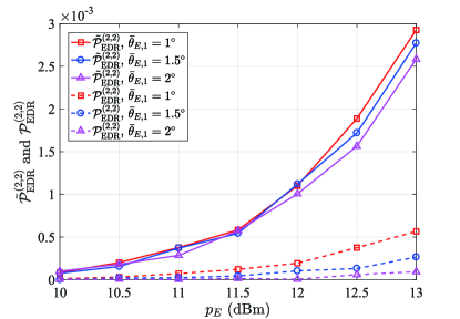
In the simulation part, we will show that 𝒫EDR(2,2)superscriptsubscript𝒫EDR22\mathcal{P}_{\mathrm{EDR}}^{(2,2)} is generally small, which means that the BS can successfully recognize 𝒚(L)superscript𝒚𝐿\bm{y}^{(L)} with high probability. Note that the calculation of T2(2)superscriptsubscript𝑇22T_{2}^{(2)} requires an inverse operation with respect to a 2Mdimensional2𝑀𝑑𝑖𝑚𝑒𝑛𝑠𝑖𝑜𝑛𝑎𝑙2M-dimensional matrix, therefore, the GLLR based method is computationally more complex than the power comparison based method.

III-D K=2𝐾2K=2 but Eve fails to hit LU’s PS, or K>2𝐾2K>2

Refer to caption
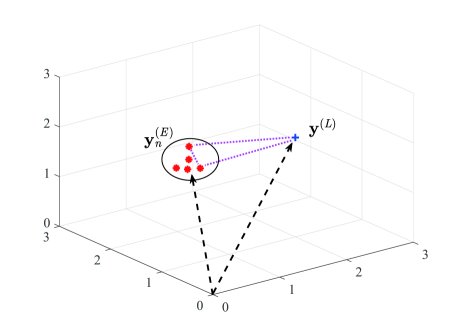
Figure 2: Basic principle of the proposed distance-based method.

In this case, we have the following two situations:

  • K>2𝐾2K>2 and Eve hits LU’s PS, and we have 𝒚(L)=𝒉L+ejω(L)βPSA(K)𝒉E+𝒛(L)ΨPSA(C)superscript𝒚𝐿subscript𝒉𝐿superscriptejsuperscript𝜔𝐿superscriptsubscript𝛽PSA𝐾subscript𝒉𝐸superscript𝒛𝐿superscriptsubscriptΨPSA𝐶\bm{y}^{(L)}=\bm{h}_{L}+\mathrm{e}^{\mathrm{j}\omega^{(L)}}\beta_{\mathrm{PSA}}^{(K)}\bm{h}_{E}+\bm{z}^{(L)}\in\Psi_{\mathrm{PSA}}^{(C)}.

  • K2𝐾2K\geq 2 but Eve fails to hit LU’s PS, and we have 𝒚(L)=𝒉L+𝒛(L)ΨPSA(C)superscript𝒚𝐿subscript𝒉𝐿superscript𝒛𝐿superscriptsubscriptΨPSA𝐶\bm{y}^{(L)}=\bm{h}_{L}+\bm{z}^{(L)}\in\Psi_{\mathrm{PSA}}^{(C)}.

Denote the channel observations in ΨPSA(C)superscriptsubscriptΨPSA𝐶\Psi_{\mathrm{PSA}}^{(C)} as {𝒚1,,𝒚QC}subscript𝒚1subscript𝒚subscript𝑄𝐶\{\bm{y}_{1},\cdots,\bm{y}_{Q_{C}}\}. For both cases listed above, the BS needs to figure out which channel observation is 𝒚(L)superscript𝒚𝐿\bm{y}^{(L)}. We propose an unified method to handle both of the two cases, regardless the value of K𝐾K. Note that we have ΨPSA(C)={𝒚(L)}ΨPSA(E)superscriptsubscriptΨPSA𝐶superscript𝒚𝐿superscriptsubscriptΨPSA𝐸\Psi_{\mathrm{PSA}}^{(C)}=\{\bm{y}^{(L)}\}\cup\Psi_{\mathrm{PSA}}^{(E)}. From (7), we observe that for a given realization of 𝒉Esubscript𝒉𝐸\bm{h}_{E}, the channel observations in ΨPSA(E)superscriptsubscriptΨPSA𝐸\Psi_{\mathrm{PSA}}^{(E)}, after some phase shifts, are clustered around βPSA(K)𝒉Esuperscriptsubscript𝛽PSA𝐾subscript𝒉𝐸\beta_{\mathrm{PSA}}^{(K)}\bm{h}_{E} in a M𝑀M–dimensional complex-valued space with relatively small biases due to the noise terms, i.e., 𝒛1(E),𝒛2(E),,𝒛QE(E)superscriptsubscript𝒛1𝐸superscriptsubscript𝒛2𝐸superscriptsubscript𝒛subscript𝑄𝐸𝐸\bm{z}_{1}^{(E)},\bm{z}_{2}^{(E)},\cdots,\bm{z}_{Q_{E}}^{(E)}. However, 𝒚(L)superscript𝒚𝐿\bm{y}^{(L)} is generally apart from βPSA(K)𝒉Esuperscriptsubscript𝛽PSA𝐾subscript𝒉𝐸\beta_{\mathrm{PSA}}^{(K)}\bm{h}_{E} due to the existence of 𝒉Lsubscript𝒉𝐿\bm{h}_{L}. This observation inspires us a novel distance-based method to determine 𝒚(L)superscript𝒚𝐿\bm{y}^{(L)}, the basic principle of which is shown in Fig 2.

III-D1 The distance-based method

For n{0,1,,QC}for-all𝑛01subscript𝑄𝐶\forall n\in\{0,1,\cdots,Q_{C}\}, define the distances between the channel observations as

dnsubscript𝑑𝑛\displaystyle d_{n} 𝕀{1nQC1}(minϕ𝒚nejϕ𝒚n+12)absentsubscript𝕀1𝑛subscript𝑄𝐶1subscriptminitalic-ϕsuperscriptnormsubscript𝒚𝑛superscriptejitalic-ϕsubscript𝒚𝑛12\displaystyle\triangleq\mathbb{I}_{\{1\leq n\leq Q_{C}-1\}}\left(\mathop{\mathrm{min}}\limits_{\phi}\left\|\bm{y}_{n}-\mathrm{e}^{\mathrm{j}\phi}\bm{y}_{n+1}\right\|^{2}\right)
+𝕀{n=0 or QC}(minϕ𝒚1ejϕ𝒚QC2).subscript𝕀𝑛0 or subscript𝑄𝐶subscriptminitalic-ϕsuperscriptnormsubscript𝒚1superscriptejitalic-ϕsubscript𝒚subscript𝑄𝐶2\displaystyle\quad+\mathbb{I}_{\{n=0\text{~{}or~{}}Q_{C}\}}\left(\mathop{\mathrm{min}}\limits_{\phi}\left\|\bm{y}_{1}-\mathrm{e}^{\mathrm{j}\phi}\bm{y}_{Q_{C}}\right\|^{2}\right). (26)

If dn>ϵsubscript𝑑𝑛italic-ϵd_{n}>\epsilon and dn1>ϵsubscript𝑑𝑛1italic-ϵd_{n-1}>\epsilon, then we conclude that 𝒚n=𝒚(L)subscript𝒚𝑛superscript𝒚𝐿\bm{y}_{n}=\bm{y}^{(L)}, and if dnϵsubscript𝑑𝑛italic-ϵd_{n}\leq\epsilon and dn1ϵsubscript𝑑𝑛1italic-ϵd_{n-1}\leq\epsilon, then we conclude that 𝒚nΨPSA(E)subscript𝒚𝑛superscriptsubscriptΨPSA𝐸\bm{y}_{n}\in\Psi_{\mathrm{PSA}}^{(E)}, where ϵitalic-ϵ\epsilon is a pre-designed threshold. Note that it is possible that dn>ϵsubscript𝑑𝑛italic-ϵd_{n}>\epsilon (dn<ϵsubscript𝑑𝑛italic-ϵd_{n}<\epsilon) while both dn1subscript𝑑𝑛1d_{n-1} and dn+1subscript𝑑𝑛1d_{n+1} are smaller (larger) than ϵitalic-ϵ\epsilon, which leads to a dilemma. Therefore, a proper threshold ϵitalic-ϵ\epsilon should be designed to keep the probabilities of these events low.

III-D2 Design the threshold ϵitalic-ϵ\epsilon

If {𝒚n,𝒚n+1}ΨPSA(E)subscript𝒚𝑛subscript𝒚𝑛1superscriptsubscriptΨPSA𝐸\{\bm{y}_{n},\bm{y}_{n+1}\}\subset\Psi_{\mathrm{PSA}}^{(E)}, we expect the probability that dnsubscript𝑑𝑛d_{n} exceeds ϵitalic-ϵ\epsilon to be as small as possible. Therefore, we choose the value of ϵitalic-ϵ\epsilon such that

𝒫F(ϵ)𝒫{dn>ϵ|{𝒚n,𝒚n+1}ΨPSA(E)}η,subscript𝒫𝐹italic-ϵ𝒫conditional-setsubscript𝑑𝑛italic-ϵsubscript𝒚𝑛subscript𝒚𝑛1superscriptsubscriptΨPSA𝐸𝜂\displaystyle\mathcal{P}_{F}\left(\epsilon\right)\triangleq\mathcal{P}\left\{d_{n}>\epsilon|\{\bm{y}_{n},\bm{y}_{n+1}\}\subset\Psi_{\mathrm{PSA}}^{(E)}\right\}\leq\eta, (27)

where η𝜂\eta (0<η<10𝜂10<\eta<1) is a pre-designed value. In fact, η𝜂\eta is analogous to the false alarm rate in a hypothesis test problem, and in general, we should set a small value of η𝜂\eta to ensure a low EDR. Note that 𝒫{dn<ϵ|𝒚n=𝒚(L) or 𝒚n+1=𝒚(L)}𝒫subscript𝑑𝑛braitalic-ϵsubscript𝒚𝑛superscript𝒚𝐿 or subscript𝒚𝑛1superscript𝒚𝐿\mathcal{P}\left\{d_{n}<\epsilon|\bm{y}_{n}=\bm{y}^{(L)}\text{~{}or~{}}\bm{y}_{n+1}=\bm{y}^{(L)}\right\} increases with ϵitalic-ϵ\epsilon, and thus, we set 𝒫F(ϵ)=ηsubscript𝒫𝐹italic-ϵ𝜂\mathcal{P}_{F}\left(\epsilon\right)=\eta to obtain the smallest decision threshold ϵitalic-ϵ\epsilon that satisfies (27).

The direct calculation of ϵitalic-ϵ\epsilon via 𝒫F(ϵ)subscript𝒫𝐹italic-ϵ\mathcal{P}_{F}\left(\epsilon\right) is difficult because there is no closed-form expression for 𝒫F(ϵ)subscript𝒫𝐹italic-ϵ\mathcal{P}_{F}\left(\epsilon\right). To deal with this problem, in the following theorem, we provide an upper bound on dnsubscript𝑑𝑛d_{n} when {𝒚n,𝒚n+1}ΨPSA(E)subscript𝒚𝑛subscript𝒚𝑛1superscriptsubscriptΨPSA𝐸\{\bm{y}_{n},\bm{y}_{n+1}\}\subset\Psi_{\mathrm{PSA}}^{(E)} to obtain a closed-form approximation of 𝒫F(ϵ)subscript𝒫𝐹italic-ϵ\mathcal{P}_{F}\left(\epsilon\right).

   Theorem 3.

A closed-form upper bound on 𝒫F(ϵ)subscript𝒫𝐹italic-ϵ\mathcal{P}_{F}\left(\epsilon\right) can be written as

𝒫F(ϵ)𝒫~F(ϵ)Γ(M,ϵ/(2σz2))/Γ(M).subscript𝒫𝐹italic-ϵsubscript~𝒫𝐹italic-ϵΓ𝑀italic-ϵ2superscriptsubscript𝜎𝑧2Γ𝑀\displaystyle\mathcal{P}_{F}\left(\epsilon\right)\leq\tilde{\mathcal{P}}_{F}\left(\epsilon\right)\triangleq\Gamma\left(M,\epsilon/(2\sigma_{z}^{2})\right)/\Gamma\left(M\right). (28)
Proof:

Conditioned on {𝒚n,𝒚n+1}ΨPSA(E)subscript𝒚𝑛subscript𝒚𝑛1superscriptsubscriptΨPSA𝐸\{\bm{y}_{n},\bm{y}_{n+1}\}\subset\Psi_{\mathrm{PSA}}^{(E)}, we have

dnsubscript𝑑𝑛\displaystyle d_{n} =minϕejωnβPSA(K)𝒉E+𝒛nabsentconditionalsubscriptminitalic-ϕsuperscriptejsubscript𝜔𝑛superscriptsubscript𝛽PSA𝐾subscript𝒉𝐸subscript𝒛𝑛\displaystyle=\mathop{\mathrm{min}}\limits_{\phi}\Big{\|}\mathrm{e}^{\mathrm{j}\omega_{n}}\beta_{\mathrm{PSA}}^{(K)}\bm{h}_{E}+\bm{z}_{n}
ejϕ(ejωn+1βPSA(K)𝒉E+𝒛n+1)2\displaystyle\quad\quad\quad\quad-\mathrm{e}^{\mathrm{j}\phi}\left(\mathrm{e}^{\mathrm{j}\omega_{n+1}}\beta_{\mathrm{PSA}}^{(K)}\bm{h}_{E}+\bm{z}_{n+1}\right)\Big{\|}^{2}
d~n𝒛nej(ωnωn+1)𝒛n+12.absentsubscript~𝑑𝑛superscriptnormsubscript𝒛𝑛superscriptejsubscript𝜔𝑛subscript𝜔𝑛1subscript𝒛𝑛12\displaystyle\leq\tilde{d}_{n}\triangleq\left\|\bm{z}_{n}-\mathrm{e}^{\mathrm{j}\left(\omega_{n}-\omega_{n+1}\right)}\bm{z}_{n+1}\right\|^{2}. (29)

In (29), (𝒛nej(ωnωn+1)𝒛n+1)(𝟎,2σz2𝑰)similar-tosubscript𝒛𝑛superscriptejsubscript𝜔𝑛subscript𝜔𝑛1subscript𝒛𝑛102superscriptsubscript𝜎𝑧2𝑰\left(\bm{z}_{n}-\mathrm{e}^{\mathrm{j}\left(\omega_{n}-\omega_{n+1}\right)}\bm{z}_{n+1}\right)\sim\mathbb{CN}\left(\bm{0},2\sigma_{z}^{2}\bm{I}\right), and thus d~n𝔾(M,2σz2)similar-tosubscript~𝑑𝑛𝔾𝑀2superscriptsubscript𝜎𝑧2\tilde{d}_{n}\sim\mathbb{G}\left(M,2\sigma_{z}^{2}\right). According to (29), the CCDF of d~nsubscript~𝑑𝑛\tilde{d}_{n}, i.e., 𝒫~F(ϵ)subscript~𝒫𝐹italic-ϵ\tilde{\mathcal{P}}_{F}\left(\epsilon\right) in (28), is an upper bound on 𝒫F(ϵ)subscript𝒫𝐹italic-ϵ\mathcal{P}_{F}\left(\epsilon\right). ∎

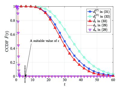
Using d~nsubscript~𝑑𝑛\tilde{d}_{n} in (29) to approximate dnsubscript𝑑𝑛d_{n} leads to an approximation of ϵitalic-ϵ\epsilon, i.e., ϵ~2σz2Γ1(M,ηΓ(M))~italic-ϵ2superscriptsubscript𝜎𝑧2superscriptΓ1𝑀𝜂Γ𝑀\tilde{\epsilon}\triangleq 2\sigma_{z}^{2}\Gamma^{-1}\left(M,\eta\Gamma\left(M\right)\right), where Γ1(M,x)superscriptΓ1𝑀𝑥\Gamma^{-1}\left(M,x\right) is the inverse function of Γ(M,x)Γ𝑀𝑥\Gamma\left(M,x\right). We show the high accuracy of using d~nsubscript~𝑑𝑛\tilde{d}_{n} to approximate dnsubscript𝑑𝑛d_{n} in Fig. 4(a) in Section VII.

III-D3 EDR analysis

Without loss of generality, assume 𝒚1=𝒚(L)subscript𝒚1superscript𝒚𝐿\bm{y}_{1}=\bm{y}^{(L)}, then the BS may make a mistake on determining 𝒚(L)superscript𝒚𝐿\bm{y}^{(L)} if one of the following events happens: (1) d1ϵsubscript𝑑1italic-ϵd_{1}\leq\epsilon, denoted by 1subscript1\mathcal{E}_{1}, (2) d0ϵsubscript𝑑0italic-ϵd_{0}\leq\epsilon, denoted by 2subscript2\mathcal{E}_{2}, and (3) k{2,3,,QC1}𝑘23subscript𝑄𝐶1\exists k\in\{2,3,\cdots,Q_{C}-1\} satisfying dk>ϵsubscript𝑑𝑘italic-ϵd_{k}>\epsilon, denoted by 3subscript3\mathcal{E}_{3}. Accordingly, the EDR can be written as 𝒫EDR𝒫{i=13i}.subscript𝒫EDR𝒫superscriptsubscript𝑖13subscript𝑖\mathcal{P}_{\mathrm{EDR}}\triangleq\mathcal{P}\left\{\bigcup_{i=1}^{3}\mathcal{E}_{i}\right\}.

In general, a tractable expression for 𝒫EDRsubscript𝒫EDR\mathcal{P}_{\mathrm{EDR}} is hard to obtain due to the fact that: (1) the PDFs of dnsubscript𝑑𝑛d_{n} for n{1,2,,QC}𝑛12subscript𝑄𝐶n\in\left\{1,2,\cdots,Q_{C}\right\} are complicated, and (2) {d0,d1,,dQC}subscript𝑑0subscript𝑑1subscript𝑑subscript𝑄𝐶\left\{d_{0},d_{1},\cdots,d_{Q_{C}}\right\} are correlated with each other. Here we consider an upper approximation of 𝒫EDRsubscript𝒫EDR\mathcal{P}_{\mathrm{EDR}}, which is given by

𝒫EDRsubscript𝒫EDR\displaystyle\mathcal{P}_{\mathrm{EDR}} =𝒫{i=13i}𝒫{1}+𝒫{2}+𝒫{3}absent𝒫superscriptsubscript𝑖13subscript𝑖𝒫subscript1𝒫subscript2𝒫subscript3\displaystyle=\mathcal{P}\left\{\cup_{i=1}^{3}\mathcal{E}_{i}\right\}\leq\mathcal{P}\left\{\mathcal{E}_{1}\right\}+\mathcal{P}\left\{\mathcal{E}_{2}\right\}+\mathcal{P}\left\{\mathcal{E}_{3}\right\}
𝒫¯EDR2𝒫{1}+η,absentsubscript¯𝒫EDR2𝒫subscript1𝜂\displaystyle\approx\overline{\mathcal{P}}_{\mathrm{EDR}}\triangleq 2\mathcal{P}\left\{\mathcal{E}_{1}\right\}+\eta, (30)

where we approximate 𝒫{3}𝒫subscript3\mathcal{P}\left\{\mathcal{E}_{3}\right\} as η𝜂\eta based on the observation that we have 𝒫{dn>ϵ}η𝒫subscript𝑑𝑛italic-ϵ𝜂\mathcal{P}\{d_{n}>\epsilon\}\leq\eta for n{2,3,,QC1}for-all𝑛23subscript𝑄𝐶1\forall n\in\left\{2,3,\cdots,Q_{C}-1\right\}, and when η𝜂\eta is small, the probability of having multiple elements in {d2,d3,,dQC1}subscript𝑑2subscript𝑑3subscript𝑑subscript𝑄𝐶1\left\{d_{2},d_{3},\cdots,d_{Q_{C}-1}\right\} larger than ϵitalic-ϵ\epsilon is negligible.

Now, to calculate 𝒫¯EDRsubscript¯𝒫EDR\overline{\mathcal{P}}_{\mathrm{EDR}} is equivalent to calculate 𝒫{d1ϵ}𝒫subscript𝑑1italic-ϵ\mathcal{P}\left\{d_{1}\leq\epsilon\right\}. However, since there is no tractable expression for the PDF of d1subscript𝑑1d_{1}, it is still very difficult if not impossible. To deal with this problem, we provide a tractable approximate of d1subscript𝑑1d_{1} as follows:

  • if 𝒚1subscript𝒚1\bm{y}_{1} is contaminated by 𝒉Esubscript𝒉𝐸\bm{h}_{E}, we denote d1subscript𝑑1d_{1} in this case as d1(C)superscriptsubscript𝑑1𝐶d_{1}^{(C)}, and then we have

    d1(C)minϕ𝒉L+ejω1βPSA(K)𝒉E+𝒛1superscriptsubscript𝑑1𝐶conditionalsubscriptminitalic-ϕsubscript𝒉𝐿superscriptejsubscript𝜔1superscriptsubscript𝛽PSA𝐾subscript𝒉𝐸subscript𝒛1\displaystyle d_{1}^{(C)}\triangleq\mathop{\mathrm{min}}\limits_{\phi}\Big{\|}\bm{h}_{L}+\mathrm{e}^{\mathrm{j}\omega_{1}}\beta_{\mathrm{PSA}}^{(K)}\bm{h}_{E}+\bm{z}_{1}
    ejϕ(ejω2βPSA(K)𝒉E+𝒛2)2\displaystyle\quad\quad\quad\quad\quad-\mathrm{e}^{\mathrm{j}\phi}\left(\mathrm{e}^{\mathrm{j}\omega_{2}}\beta_{\mathrm{PSA}}^{(K)}\bm{h}_{E}+\bm{z}_{2}\right)\Big{\|}^{2}
    \displaystyle\approx\ d~1(C)minϕ𝒉L+𝒛1𝒛~2superscriptsubscript~𝑑1𝐶conditionalsubscriptminitalic-ϕsubscript𝒉𝐿subscript𝒛1subscript~𝒛2\displaystyle\tilde{d}_{1}^{(C)}\triangleq\mathop{\mathrm{min}}\limits_{\phi}\Big{\|}\bm{h}_{L}+\bm{z}_{1}-\tilde{\bm{z}}_{2}
    +(ejω1ejϕejω2)βPSA(K)𝒉E2,\displaystyle\quad\quad\quad\quad\quad+\left(\mathrm{e}^{\mathrm{j}\omega_{1}}-\mathrm{e}^{\mathrm{j}\phi}\mathrm{e}^{\mathrm{j}\omega_{2}}\right)\beta_{\mathrm{PSA}}^{(K)}\bm{h}_{E}\Big{\|}^{2}, (31)
  • if 𝒚1subscript𝒚1\bm{y}_{1} is not contaminated by 𝒉Esubscript𝒉𝐸\bm{h}_{E}, we denote d1subscript𝑑1d_{1} in this case as d1(N)superscriptsubscript𝑑1𝑁d_{1}^{(N)}, and then we have

    d1(N)minϕ𝒉L+𝒛1ejϕ(ejω2βPSA(K)𝒉E+𝒛2)2superscriptsubscript𝑑1𝑁subscriptminitalic-ϕsuperscriptnormsubscript𝒉𝐿subscript𝒛1superscriptejitalic-ϕsuperscriptejsubscript𝜔2superscriptsubscript𝛽PSA𝐾subscript𝒉𝐸subscript𝒛22\displaystyle d_{1}^{(N)}\triangleq\mathop{\mathrm{min}}\limits_{\phi}\left\|\bm{h}_{L}+\bm{z}_{1}-\mathrm{e}^{\mathrm{j}\phi}\left(\mathrm{e}^{\mathrm{j}\omega_{2}}\beta_{\mathrm{PSA}}^{(K)}\bm{h}_{E}+\bm{z}_{2}\right)\right\|^{2}
    \displaystyle\approx\ d~1(N)minϕ𝒉L+𝒛1𝒛~2ejϕejω2βPSA(K)𝒉E2,superscriptsubscript~𝑑1𝑁subscriptminitalic-ϕsuperscriptnormsubscript𝒉𝐿subscript𝒛1subscript~𝒛2superscriptejitalic-ϕsuperscriptejsubscript𝜔2superscriptsubscript𝛽PSA𝐾subscript𝒉𝐸2\displaystyle\tilde{d}_{1}^{(N)}\triangleq\mathop{\mathrm{min}}\limits_{\phi}\left\|\bm{h}_{L}+\bm{z}_{1}-\tilde{\bm{z}}_{2}-\mathrm{e}^{\mathrm{j}\phi}\mathrm{e}^{\mathrm{j}\omega_{2}}\beta_{\mathrm{PSA}}^{(K)}\bm{h}_{E}\right\|^{2}, (32)

where the approximations in (31) and (32) is obtained by replacing ejϕ𝒛2superscriptejitalic-ϕsubscript𝒛2\mathrm{e}^{\mathrm{j}\phi}\boldsymbol{z}_{2} with 𝒛~2(𝟎,σz2𝑰M)similar-tosubscript~𝒛20superscriptsubscript𝜎𝑧2subscript𝑰𝑀\tilde{\boldsymbol{z}}_{2}\sim\mathbb{CN}\left(\boldsymbol{0},\sigma_{z}^{2}\boldsymbol{I}_{M}\right) which is independent of ϕitalic-ϕ\phi. Both of d~1(C)superscriptsubscript~𝑑1𝐶\tilde{d}_{1}^{(C)} and d~1(N)superscriptsubscript~𝑑1𝑁\tilde{d}_{1}^{(N)} are further lower bounded by

d~1(i)superscriptsubscript~𝑑1𝑖\displaystyle\tilde{d}_{1}^{(i)} minx𝒉L+𝒛x𝒉E2absentsubscriptmin𝑥superscriptnormsubscript𝒉𝐿𝒛𝑥subscript𝒉𝐸2\displaystyle\geq\mathop{\mathrm{min}}\limits_{x}\left\|\bm{h}_{L}+\bm{z}-x\bm{h}_{E}\right\|^{2}
=𝒉L+𝒛2|𝒉EH(𝒉L+𝒛)|2𝒉E2absentsuperscriptnormsubscript𝒉𝐿𝒛2superscriptsuperscriptsubscript𝒉𝐸𝐻subscript𝒉𝐿𝒛2superscriptnormsubscript𝒉𝐸2\displaystyle=\left\|\bm{h}_{L}+\bm{z}\right\|^{2}-\frac{\left|\bm{h}_{E}^{H}\left(\bm{h}_{L}+\bm{z}\right)\right|^{2}}{\left\|\bm{h}_{E}\right\|^{2}}
(a)d^1(𝒉L+𝒛)H𝑸(𝒉L+𝒛),i{C,N},formulae-sequence𝑎subscript^𝑑1superscriptsubscript𝒉𝐿𝒛𝐻𝑸subscript𝒉𝐿𝒛𝑖𝐶𝑁\displaystyle\overset{(a)}{\approx}\hat{d}_{1}\triangleq\left(\bm{h}_{L}+\bm{z}\right)^{H}\bm{Q}\left(\bm{h}_{L}+\bm{z}\right),\quad i\in\{C,N\}, (33)

where 𝒛𝒛1𝒛~2𝒛subscript𝒛1subscript~𝒛2\bm{z}\triangleq\bm{z}_{1}-\tilde{\bm{z}}_{2}, 𝑸𝑰𝑹ETr(𝑹E)𝑸𝑰subscript𝑹𝐸Trsubscript𝑹𝐸\bm{Q}\triangleq\bm{I}-\frac{\bm{R}_{E}}{\mathrm{Tr}\left(\bm{R}_{E}\right)}, and step (a)𝑎(a) is obtained by using 𝒉E𝒉EH𝒉E2𝑹ETr(𝑹E)subscript𝒉𝐸superscriptsubscript𝒉𝐸𝐻superscriptnormsubscript𝒉𝐸2subscript𝑹𝐸Trsubscript𝑹𝐸\frac{\bm{h}_{E}\bm{h}_{E}^{H}}{\left\|\bm{h}_{E}\right\|^{2}}\rightarrow\frac{\bm{R}_{E}}{\mathrm{Tr}\left(\bm{R}_{E}\right)} when M𝑀M is large.

According to (33), we can approximate 𝒫{1}𝒫subscript1\mathcal{P}\left\{\mathcal{E}_{1}\right\} by 𝒫{d^1ϵ}𝒫subscript^𝑑1italic-ϵ\mathcal{P}\left\{\hat{d}_{1}\leq\epsilon\right\}, and the calculation of 𝒫{d^1ϵ}𝒫subscript^𝑑1italic-ϵ\mathcal{P}\left\{\hat{d}_{1}\leq\epsilon\right\} is provided in the following theorem.

   Theorem 4.

𝒫{d^1ϵ}𝒫subscript^𝑑1italic-ϵ\mathcal{P}\left\{\hat{d}_{1}\leq\epsilon\right\} can be calculated as

𝒫{d^1ϵ}=𝒫{𝜶H𝑸¯𝜶ϵ},𝒫subscript^𝑑1italic-ϵ𝒫superscript𝜶𝐻¯𝑸𝜶italic-ϵ\displaystyle\mathcal{P}\left\{\hat{d}_{1}\leq\epsilon\right\}=\mathcal{P}\left\{\bm{\alpha}^{H}\bar{\bm{Q}}\bm{\alpha}\leq\epsilon\right\}, (34)

where 𝜶(𝟎,𝑰M)similar-to𝜶0subscript𝑰𝑀\bm{\alpha}\sim\mathbb{CN}\left(\bm{0},\bm{I}_{M}\right), and 𝑸¯(𝑹L+2σz2𝑰M)12𝑸(𝑹L+2σz2𝑰M)12¯𝑸superscriptsubscript𝑹𝐿2superscriptsubscript𝜎𝑧2subscript𝑰𝑀12𝑸superscriptsubscript𝑹𝐿2superscriptsubscript𝜎𝑧2subscript𝑰𝑀12\bar{\bm{Q}}\triangleq\left(\bm{R}_{L}+2\sigma_{z}^{2}\boldsymbol{I}_{M}\right)^{\frac{1}{2}}\bm{Q}\left(\bm{R}_{L}+2\sigma_{z}^{2}\boldsymbol{I}_{M}\right)^{\frac{1}{2}}.

Proof:

The proof is similar to that of Theorem 1, and thus is omitted. ∎

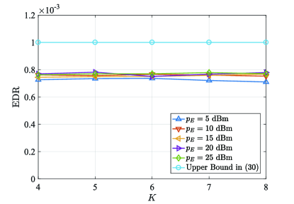
We plot the CCDF of d1(C)superscriptsubscript𝑑1𝐶d_{1}^{(C)},d1(N)superscriptsubscript𝑑1𝑁d_{1}^{(N)}, and d^1subscript^𝑑1\hat{d}_{1} in Fig. 4(a) to show that d1(N)superscriptsubscript𝑑1𝑁d_{1}^{(N)} is a satisfying lower approximation of both d1(C)superscriptsubscript𝑑1𝐶d_{1}^{(C)} and d1(N)superscriptsubscript𝑑1𝑁d_{1}^{(N)}. And we also compare 𝒫EDRsubscript𝒫EDR\mathcal{P}_{\mathrm{EDR}} obtained from simulation with its analytical upper approximation 𝒫¯EDRsubscript¯𝒫EDR\overline{\mathcal{P}}_{\mathrm{EDR}} in (30) in Section VII.

III-E If K𝐾K is unknown by the BS

We have discussed the cases when K𝐾K is known by the BS in the previous subsections. In practice, K𝐾K is chosen by Eve and the BS generally does not have any prior information on K𝐾K. However, even though the BS does not know the value of K𝐾K, we will show that in order to identify 𝒚(L)superscript𝒚𝐿\bm{y}^{(L)}, the BS only needs to carry out some additional operations to decide whether a hit event happens. And then, all the discussions in the previous subsections hold as well. In the following, the detailed discussions on these additional operations are provided. For simplicity and clarity, we classify the discussions according to the value of QCsubscript𝑄𝐶Q_{C}.

III-E1 QC=1subscript𝑄𝐶1Q_{C}=1

In this case, ΨPSA(C)={𝒚(L)}superscriptsubscriptΨPSA𝐶superscript𝒚𝐿\Psi_{\mathrm{PSA}}^{(C)}=\left\{\bm{y}^{(L)}\right\}, and the BS needs to distinguish between:

  • (0,1)superscript01\mathcal{H}^{(0,1)}: K=0𝐾0K=0, i.e., Eve keeps silent,

  • (1,1)superscript11\mathcal{H}^{(1,1)}: K=1𝐾1K=1 and Eve successfully hits LU’s PS.

Note that to distinguish between (0,1)superscript01\mathcal{H}^{(0,1)} and (1,1)superscript11\mathcal{H}^{(1,1)} is equivalent to detect the existence of PSA under the conventional channel training scheme wherein only one PS is assigned to the LU as discussed in [26, 25, 24, 23, 22]. And this can be easily realized by checking the LLR, i.e.,

lnp{𝒚(L)|(0,1)}lnp{𝒚(L)|(1,1)}(1,1)(0,1)0,superscriptsubscriptgreater-than-or-equals-or-less-thansuperscript11superscript01𝑝conditional-setsuperscript𝒚𝐿superscript01𝑝conditional-setsuperscript𝒚𝐿superscript110\displaystyle\ln p\left\{\bm{y}^{(L)}|\mathcal{H}^{(0,1)}\right\}-\ln p\left\{\bm{y}^{(L)}|\mathcal{H}^{(1,1)}\right\}{\gtreqless}_{\mathcal{H}^{(1,1)}}^{\mathcal{H}^{(0,1)}}0, (35)

where 𝒚(L)(𝟎,𝑹L,z)similar-tosuperscript𝒚𝐿0subscript𝑹𝐿𝑧\bm{y}^{(L)}\sim\mathbb{CN}\left(\bm{0},\bm{R}_{L,z}\right) conditioned on 0subscript0\mathcal{H}_{0}, and 𝒚(L)(𝟎,𝑹L,E,z(1))similar-tosuperscript𝒚𝐿0superscriptsubscript𝑹𝐿𝐸𝑧1\bm{y}^{(L)}\sim\mathbb{CN}\left(\bm{0},\bm{R}_{L,E,z}^{(1)}\right) conditioned on 1subscript1\mathcal{H}_{1}.

III-E2 QC=2subscript𝑄𝐶2Q_{C}=2

The following two situations will result in QC=2subscript𝑄𝐶2Q_{C}=2, i.e.,

  • (1,2)superscript12\mathcal{H}^{(1,2)}: K=1𝐾1K=1, but Eve fails to hit LU’s PS,

  • (2,2)superscript22\mathcal{H}^{(2,2)}: K=2𝐾2K=2, and Eve successfully hits LU’s PS.

To distinguish between (1,2)superscript12\mathcal{H}^{(1,2)} and (2,2)superscript22\mathcal{H}^{(2,2)}, we first determine the subcases of (1,2)superscript12\mathcal{H}^{(1,2)}, i.e., 0(1,2)superscriptsubscript012\mathcal{H}_{0}^{(1,2)} and 1(1,2)superscriptsubscript112\mathcal{H}_{1}^{(1,2)} defined in Section III-B, by using the method provided in Section III-B. Assume the decision result between 0(1,2)superscriptsubscript012\mathcal{H}_{0}^{(1,2)} and 1(1,2)superscriptsubscript112\mathcal{H}_{1}^{(1,2)} is denoted by j1(1,2)superscriptsubscriptsubscript𝑗112\mathcal{H}_{j_{1}}^{(1,2)} where j1=argmaxi=0,1p(𝒈|i(1,2))subscript𝑗1subscriptargmax𝑖01𝑝conditional𝒈superscriptsubscript𝑖12j_{1}=\mathrm{argmax}_{i=0,1}~{}p\left(\bm{g}|\mathcal{H}_{i}^{(1,2)}\right). Then, we determine the subcases of (2,2)superscript22\mathcal{H}^{(2,2)}, i.e., 0(2,2)superscriptsubscript022\mathcal{H}_{0}^{(2,2)} and 1(2,2)superscriptsubscript122\mathcal{H}_{1}^{(2,2)} defined in Section III-C, by using the method provided in Section III-C (both the power comparison based method and the GLLR based method are applicable). If the GLLR based method is used, then we denote the decision result between 0(2,2)superscriptsubscript022\mathcal{H}_{0}^{(2,2)} and 1(2,2)superscriptsubscript122\mathcal{H}_{1}^{(2,2)} as j2(2,2)superscriptsubscriptsubscript𝑗222\mathcal{H}_{j_{2}}^{(2,2)}, where j2=argmaxi=0,1(maxω(L),ω(E)p(𝒈|i(2,2)))subscript𝑗2subscriptargmax𝑖01subscriptmaxsuperscript𝜔𝐿superscript𝜔𝐸𝑝conditional𝒈superscriptsubscript𝑖22j_{2}=\mathrm{argmax}_{i=0,1}\left(\mathrm{max}_{\omega^{(L)},\omega^{(E)}}~{}p\left(\bm{g}|\mathcal{H}_{i}^{(2,2)}\right)\right). After obtaining j1(1,2)superscriptsubscriptsubscript𝑗112\mathcal{H}_{j_{1}}^{(1,2)} and j2(2,2)superscriptsubscriptsubscript𝑗222\mathcal{H}_{j_{2}}^{(2,2)}, we now resort to GLLR test to determine which one of (1,2)superscript12\mathcal{H}^{(1,2)} and (2,2)superscript22\mathcal{H}^{(2,2)} is true, i.e., ln(maxω(L),ω(E)p(𝒈|j2(2,2)))lnp(𝒈|j1(1,2))(1,2)(2,2)0superscriptsubscriptgreater-than-or-equals-or-less-thansuperscript12superscript22subscriptmaxsuperscript𝜔𝐿superscript𝜔𝐸𝑝conditional𝒈superscriptsubscriptsubscript𝑗222𝑝conditional𝒈superscriptsubscriptsubscript𝑗1120\ln\left(\mathrm{max}_{\omega^{(L)},\omega^{(E)}}~{}p\left(\bm{g}|\mathcal{H}_{j_{2}}^{(2,2)}\right)\right)-\ln p\left(\bm{g}|\mathcal{H}_{j_{1}}^{(1,2)}\right)\gtreqless_{\mathcal{H}^{(1,2)}}^{\mathcal{H}^{(2,2)}}0.

III-E3 QC>2subscript𝑄𝐶2Q_{C}>2

In this cases, we can first recognize which channel observation in ΨPSA(C)superscriptsubscriptΨPSA𝐶\Psi_{\mathrm{PSA}}^{(C)} is 𝒚(L)superscript𝒚𝐿\bm{y}^{(L)} by using the distance-based method proposed in Section III-D. After obtaining 𝒚(L)superscript𝒚𝐿\bm{y}^{(L)}, we only need to determine whether Eve hits LU’s PS, which can be simply realized by checking the LLR which is similar to that in (35).

Combining all these steps in the discussions above, we can determine which PS is 𝒙(L)superscript𝒙𝐿\bm{x}^{(L)} (which channel observation is 𝒚(L)superscript𝒚𝐿\bm{y}^{(L)}), even when K𝐾K is unknown by the BS.

IV Channel Estimation under PSA

After determining which PS is 𝒙(L)superscript𝒙𝐿\bm{x}^{(L)}, now the BS can estimate both of the legitimate and illegitimate channels.

IV-A Estimation of the legitimate channel

Assume minimum mean square error (MMSE) estimator is used at the BS, then the estimation of LU’s channel and corresponding the mean square error (MSE) matrices are given by

𝒉^Lsubscript^𝒉𝐿\displaystyle\hat{\bm{h}}_{L} =𝕀{𝒙(L)ΦE}𝑹L(𝑹L,E,z(K))1𝒚(L)absentsubscript𝕀superscript𝒙𝐿subscriptΦ𝐸subscript𝑹𝐿superscriptsuperscriptsubscript𝑹𝐿𝐸𝑧𝐾1superscript𝒚𝐿\displaystyle=\mathbb{I}_{\{\bm{x}^{(L)}\in\Phi_{E}\}}\bm{R}_{L}\left(\bm{R}_{L,E,z}^{(K)}\right)^{-1}\bm{y}^{(L)}
+𝕀{𝒙(L)ΦE}𝑹L(𝑹L,z)1𝒚(L),subscript𝕀superscript𝒙𝐿subscriptΦ𝐸subscript𝑹𝐿superscriptsubscript𝑹𝐿𝑧1superscript𝒚𝐿\displaystyle\quad+\mathbb{I}_{\{\bm{x}^{(L)}\notin\Phi_{E}\}}\bm{R}_{L}\left(\bm{R}_{L,z}\right)^{-1}\bm{y}^{(L)}, (36)
𝑹~Lsubscript~𝑹𝐿\displaystyle\tilde{\bm{R}}_{L} =𝔼{(𝒉L𝒉^L)(𝒉L𝒉^L)H}absent𝔼subscript𝒉𝐿subscript^𝒉𝐿superscriptsubscript𝒉𝐿subscript^𝒉𝐿𝐻\displaystyle=\mathbb{E}\left\{\left(\bm{h}_{L}-\hat{\bm{h}}_{L}\right)\left(\bm{h}_{L}-\hat{\bm{h}}_{L}\right)^{H}\right\}
=𝕀{𝒙(L)ΦE}(𝑹L𝑹L(𝑹L,E,z(K))1𝑹L)absentsubscript𝕀superscript𝒙𝐿subscriptΦ𝐸subscript𝑹𝐿subscript𝑹𝐿superscriptsuperscriptsubscript𝑹𝐿𝐸𝑧𝐾1subscript𝑹𝐿\displaystyle=\mathbb{I}_{\{\bm{x}^{(L)}\in\Phi_{E}\}}\left(\bm{R}_{L}-\bm{R}_{L}\left(\bm{R}_{L,E,z}^{(K)}\right)^{-1}\bm{R}_{L}\right)
+𝕀{𝒙(L)ΦE}(𝑹L𝑹L(𝑹L,z)1𝑹L).subscript𝕀superscript𝒙𝐿subscriptΦ𝐸subscript𝑹𝐿subscript𝑹𝐿superscriptsubscript𝑹𝐿𝑧1subscript𝑹𝐿\displaystyle\quad+\mathbb{I}_{\{\bm{x}^{(L)}\notin\Phi_{E}\}}\left(\bm{R}_{L}-\bm{R}_{L}\left(\bm{R}_{L,z}\right)^{-1}\bm{R}_{L}\right). (37)

IV-B Estimation of illegitimate channel

To estimate the channel of Eve, we consider the following two situations:

IV-B1 QC=1subscript𝑄𝐶1Q_{C}=1 and PSA is detected

In this case, the only one channel observation in ΨCsubscriptΨ𝐶\Psi_{C} is 𝒚(L)=𝒉L+ejω(L)βPSA(1)𝒉E+𝒛(L)superscript𝒚𝐿subscript𝒉𝐿superscriptejsuperscript𝜔𝐿superscriptsubscript𝛽PSA1subscript𝒉𝐸superscript𝒛𝐿\bm{y}^{(L)}=\bm{h}_{L}+\mathrm{e}^{\mathrm{j}\omega^{(L)}}\beta_{\mathrm{PSA}}^{(1)}\bm{h}_{E}+\bm{z}^{(L)}, and therefore, the estimation of Eve’s channel444We have to point out here that the estimated illegitimate channel, i.e., 𝒉^Esubscript^𝒉𝐸\hat{\bm{h}}_{E}, is, in fact, not an estimation of 𝒉Esubscript𝒉𝐸\bm{h}_{E} but an estimation of the entirety of the product of ejω(L)superscriptejsuperscript𝜔L\mathrm{e}^{\mathrm{j\omega^{(L)}}} and 𝒉Esubscript𝒉𝐸\bm{h}_{E}, i.e., ejω(L)𝒉Esuperscriptejsuperscript𝜔𝐿subscript𝒉𝐸\mathrm{e}^{\mathrm{j}\omega^{(L)}}\bm{h}_{E}. Due to the fact that 𝒉Esubscript𝒉𝐸\bm{h}_{E} is a circular symmetrical complex random vector, ejω(L)𝒉Esuperscriptejsuperscript𝜔𝐿subscript𝒉𝐸\mathrm{e}^{\mathrm{j}\omega^{(L)}}\bm{h}_{E} has the same distribution as 𝒉Esubscript𝒉𝐸\bm{h}_{E}, even though ω(L)superscript𝜔𝐿\omega^{(L)} is unknown. and the corresponding MSE matrix are given by

𝒉^Esubscript^𝒉𝐸\displaystyle\hat{\bm{h}}_{E} =βPSA(1)𝑹E(𝑹L,E,z(1))1𝒚(L),absentsuperscriptsubscript𝛽PSA1subscript𝑹𝐸superscriptsuperscriptsubscript𝑹𝐿𝐸𝑧11superscript𝒚𝐿\displaystyle=\beta_{\mathrm{PSA}}^{(1)}\bm{R}_{E}\left(\bm{R}_{L,E,z}^{(1)}\right)^{-1}\bm{y}^{(L)}, (38)
𝑹~Esubscript~𝑹𝐸\displaystyle\tilde{\bm{R}}_{E} =𝔼{(ejω(L)𝒉E𝒉^E)(ejω(L)𝒉E𝒉^E)H}absent𝔼superscriptejsuperscript𝜔𝐿subscript𝒉𝐸subscript^𝒉𝐸superscriptsuperscriptejsuperscript𝜔𝐿subscript𝒉𝐸subscript^𝒉𝐸𝐻\displaystyle=\mathbb{E}\left\{\left(\mathrm{e}^{\mathrm{j}\omega^{(L)}}\bm{h}_{E}-\hat{\bm{h}}_{E}\right)\left(\mathrm{e}^{\mathrm{j}\omega^{(L)}}\bm{h}_{E}-\hat{\bm{h}}_{E}\right)^{H}\right\}
=𝑹E|βPSA(1)|2𝑹E(𝑹L,E,z(1))1𝑹E.absentsubscript𝑹𝐸superscriptsuperscriptsubscript𝛽PSA12subscript𝑹𝐸superscriptsuperscriptsubscript𝑹𝐿𝐸𝑧11subscript𝑹𝐸\displaystyle=\bm{R}_{E}-\left|\beta_{\mathrm{PSA}}^{(1)}\right|^{2}\bm{R}_{E}\left(\bm{R}_{L,E,z}^{(1)}\right)^{-1}\bm{R}_{E}. (39)

IV-B2 QC>1subscript𝑄𝐶1Q_{C}>1

In this case, we can estimate 𝒉Esubscript𝒉𝐸\bm{h}_{E} from the channel observations in ΨPSA(E)superscriptsubscriptΨPSA𝐸\Psi_{\mathrm{PSA}}^{(E)}. Denote the channel observations in ΨPSA(E)superscriptsubscriptΨPSA𝐸\Psi_{\mathrm{PSA}}^{(E)} as 𝒚i(E)=βPSA(K)𝒉E(i)+𝒛i(E)superscriptsubscript𝒚𝑖𝐸superscriptsubscript𝛽PSA𝐾superscriptsubscript𝒉𝐸𝑖superscriptsubscript𝒛𝑖𝐸\bm{y}_{i}^{(E)}=\beta_{\mathrm{PSA}}^{(K)}\bm{h}_{E}^{(i)}+\bm{z}_{i}^{(E)}, for i=1,2,,QE𝑖12subscript𝑄𝐸i=1,2,\cdots,Q_{E}, where we have 𝒉E(i)ejωi(E)𝒉Esuperscriptsubscript𝒉𝐸𝑖superscriptejsuperscriptsubscript𝜔𝑖𝐸subscript𝒉𝐸\bm{h}_{E}^{(i)}\triangleq\mathrm{e}^{\mathrm{j}\omega_{i}^{(E)}}\bm{h}_{E}. To estimate the illegitimate channel, we first combine 𝒚1(E),𝒚2(E),,𝒚QE(E)superscriptsubscript𝒚1𝐸superscriptsubscript𝒚2𝐸superscriptsubscript𝒚subscript𝑄𝐸𝐸\bm{y}_{1}^{(E)},\bm{y}_{2}^{(E)},\cdots,\bm{y}_{Q_{E}}^{(E)} as

𝒚E1QEi=1QEκi𝒚i(E)=1QEi=1QEκiβPSA(K)𝒉E(i)+𝒛~E,subscript𝒚𝐸1subscript𝑄𝐸superscriptsubscript𝑖1subscript𝑄𝐸subscript𝜅𝑖superscriptsubscript𝒚𝑖𝐸1subscript𝑄𝐸superscriptsubscript𝑖1subscript𝑄𝐸subscript𝜅𝑖superscriptsubscript𝛽PSA𝐾superscriptsubscript𝒉𝐸𝑖subscript~𝒛𝐸\displaystyle\bm{y}_{E}\triangleq\frac{1}{Q_{E}}\sum_{i=1}^{Q_{E}}\kappa_{i}\bm{y}_{i}^{(E)}=\frac{1}{Q_{E}}\sum_{i=1}^{Q_{E}}\kappa_{i}\beta_{\mathrm{PSA}}^{(K)}\bm{h}_{E}^{(i)}+\tilde{\bm{z}}_{E}, (40)

where κi𝒚1(E),𝒚i(E)/|𝒚1(E),𝒚i(E)|subscript𝜅𝑖superscriptsubscript𝒚1𝐸superscriptsubscript𝒚𝑖𝐸superscriptsubscript𝒚1𝐸superscriptsubscript𝒚𝑖𝐸\kappa_{i}\triangleq\langle\bm{y}_{1}^{(E)},\bm{y}_{i}^{(E)}\rangle\big{/}|\langle\bm{y}_{1}^{(E)},\bm{y}_{i}^{(E)}\rangle|, for i=1,2,,QE𝑖12subscript𝑄𝐸i=1,2,\cdots,Q_{E}, are the combination coefficients, and 𝒛~E1QEi=1QEκi𝒛i(E)subscript~𝒛𝐸1subscript𝑄𝐸superscriptsubscript𝑖1subscript𝑄𝐸subscript𝜅𝑖superscriptsubscript𝒛𝑖𝐸\tilde{\bm{z}}_{E}\triangleq\frac{1}{Q_{E}}\sum_{i=1}^{Q_{E}}\kappa_{i}\bm{z}_{i}^{(E)} is the noise term. Note that the exact distribution of 𝒛~Esubscript~𝒛𝐸\tilde{\bm{z}}_{E}, or even its covariance matrix, is very hard to obtain because the combination coefficients, i.e., {κi}i=1QEsuperscriptsubscriptsubscript𝜅𝑖𝑖1subscript𝑄𝐸\{\kappa_{i}\}_{i=1}^{Q_{E}}, are determined by {𝒚i(E)}i=1QEsuperscriptsubscriptsuperscriptsubscript𝒚𝑖𝐸𝑖1subscript𝑄𝐸\{\bm{y}_{i}^{(E)}\}_{i=1}^{Q_{E}} in a extremely complicated form. However, we observe that the noise floor of 𝒛i(E)superscriptsubscript𝒛𝑖𝐸\bm{z}_{i}^{(E)} decreases with the increase of τ𝜏\tau and pLsubscript𝑝𝐿p_{L}, and when τ𝜏\tau and pLsubscript𝑝𝐿p_{L} is sufficiently large, it reasonable to approximate κisubscript𝜅𝑖\kappa_{i} as κiκ~iej(ω1(E)ωi(E))subscript𝜅𝑖subscript~𝜅𝑖superscriptejsuperscriptsubscript𝜔1𝐸superscriptsubscript𝜔𝑖𝐸\kappa_{i}\approx\tilde{\kappa}_{i}\triangleq\mathrm{e}^{\mathrm{j}\left(\omega_{1}^{(E)}-\omega_{i}^{(E)}\right)}. Based on κ~isubscript~𝜅𝑖\tilde{\kappa}_{i}, we have 𝔼{𝒛i(E)(𝒛i(E))H}σz2QE𝑰M𝔼superscriptsubscript𝒛𝑖𝐸superscriptsuperscriptsubscript𝒛𝑖𝐸𝐻superscriptsubscript𝜎𝑧2subscript𝑄𝐸subscript𝑰𝑀\mathbb{E}\left\{\bm{z}_{i}^{(E)}\left(\bm{z}_{i}^{(E)}\right)^{H}\right\}\approx\frac{\sigma_{z}^{2}}{Q_{E}}\bm{I}_{M}. Inserting κiκ~isubscript𝜅𝑖subscript~𝜅𝑖\kappa_{i}\approx\tilde{\kappa}_{i} into (40), we obtain 𝒚EβPSA(K)𝒉E(1)+𝒛~Esubscript𝒚𝐸superscriptsubscript𝛽PSA𝐾superscriptsubscript𝒉𝐸1subscript~𝒛𝐸\bm{y}_{E}\approx\beta_{\mathrm{PSA}}^{(K)}\bm{h}_{E}^{(1)}+\tilde{\bm{z}}_{E}. Using the linear MMSE estimator to estimate the illegitimate channel, we have

𝒉^Esubscript^𝒉𝐸\displaystyle\hat{\bm{h}}_{E} =βPSA(K)𝑹E(𝑹E(K)+σz2QE𝑰M)1𝒚E,absentsuperscriptsubscript𝛽PSA𝐾subscript𝑹𝐸superscriptsuperscriptsubscript𝑹𝐸𝐾superscriptsubscript𝜎𝑧2subscript𝑄𝐸subscript𝑰𝑀1subscript𝒚𝐸\displaystyle=\beta_{\mathrm{PSA}}^{(K)}\bm{R}_{E}\left(\bm{R}_{E}^{(K)}+\frac{\sigma_{z}^{2}}{Q_{E}}\bm{I}_{M}\right)^{-1}\bm{y}_{E}, (41)
𝑹~Esubscript~𝑹𝐸\displaystyle\tilde{\bm{R}}_{E} =𝑹E|βPSA(K)|2𝑹E(𝑹E(K)+σz2QE𝑰M)1𝑹E.absentsubscript𝑹𝐸superscriptsuperscriptsubscript𝛽PSA𝐾2subscript𝑹𝐸superscriptsuperscriptsubscript𝑹𝐸𝐾superscriptsubscript𝜎𝑧2subscript𝑄𝐸subscript𝑰𝑀1subscript𝑹𝐸\displaystyle=\bm{R}_{E}-\left|\beta_{\mathrm{PSA}}^{(K)}\right|^{2}\bm{R}_{E}\left(\bm{R}_{E}^{(K)}+\frac{\sigma_{z}^{2}}{Q_{E}}\bm{I}_{M}\right)^{-1}\bm{R}_{E}. (42)

V Secure Transmission under PSA

After UCTP, based on the channel estimations, SB vector is designed to transmit the confidential messages. Denote the signals received by the LU and Eve during DDTP as yLsubscript𝑦𝐿y_{L} and yEsubscript𝑦𝐸y_{E}, respectively, then yqsubscript𝑦𝑞y_{q} for q{L,E}𝑞𝐿𝐸q\in\{L,E\} can be written as

yqsubscript𝑦𝑞\displaystyle y_{q} =pB(𝒉^q+𝒉~q)H𝒗x+nq,absentsubscript𝑝𝐵superscriptsubscript^𝒉𝑞subscript~𝒉𝑞𝐻𝒗𝑥subscript𝑛𝑞\displaystyle=\sqrt{p_{B}}\left(\hat{\bm{h}}_{q}+\tilde{\bm{h}}_{q}\right)^{H}\bm{v}x+n_{q}, (43)

where 𝒉^qsubscript^𝒉𝑞\hat{\bm{h}}_{q} for q{L,E}𝑞𝐿𝐸q\in\{L,E\} are the estimations of the legitimate and illegitimate channels, respectively, 𝒉~q𝒉q𝒉^qsubscript~𝒉𝑞subscript𝒉𝑞subscript^𝒉𝑞\tilde{\bm{h}}_{q}\triangleq\bm{h}_{q}-\hat{\bm{h}}_{q} for q{L,E}𝑞𝐿𝐸q\in\{L,E\} are the corresponding estimation errors, nq(0,σq2)similar-tosubscript𝑛𝑞0superscriptsubscript𝜎𝑞2n_{q}\sim\mathbb{CN}\left(0,\sigma_{q}^{2}\right) for q{L,E}𝑞𝐿𝐸q\in\{L,E\} are the additive white Gaussian noises, 𝒗𝒗\bm{v} satisfying 𝒗=1norm𝒗1\left\|\bm{v}\right\|=1 is the SB vector designed by the BS, x(0,1)similar-to𝑥01x\sim\mathbb{CN}\left(0,1\right) is the confidential signal, and pBsubscript𝑝𝐵p_{B} is the power budget of the BS. Note that if positive secrecy rate exists, maximum power is optimal [33].

We make an reasonable assumption here that the LU and Eve can know their equivalent channel coefficients, i.e., (𝒉^L+𝒉~L)H𝒗superscriptsubscript^𝒉𝐿subscript~𝒉𝐿𝐻𝒗\left(\hat{\bm{h}}_{L}+\tilde{\bm{h}}_{L}\right)^{H}\bm{v} and (𝒉^E+𝒉~E)H𝒗superscriptsubscript^𝒉𝐸subscript~𝒉𝐸𝐻𝒗\left(\hat{\bm{h}}_{E}+\tilde{\bm{h}}_{E}\right)^{H}\bm{v}, when they decode the information-bearing symbols. This assumption can be realized in the following two ways,

  • after obtaining the beamforming vector 𝒗𝒗\bm{v}, the BS performs a downlink training procedure to let the LU estimate its equivalent channel coefficient.

  • note that the equivalent channel is only a complex number, and the LU may direct learn it through the received signal symbols during the whole DDTP.

Based on this assumption, the SNRSNR\mathrm{SNR} of the LU and Eve can be written, respectively, as SNRL=pB|𝒗H(𝒉^L+𝒉~L)|2σL2subscriptSNR𝐿subscript𝑝𝐵superscriptsuperscript𝒗𝐻subscript^𝒉𝐿subscript~𝒉𝐿2superscriptsubscript𝜎𝐿2\mathrm{SNR}_{L}=\frac{p_{B}\left|\bm{v}^{H}\left(\hat{\bm{h}}_{L}+\tilde{\bm{h}}_{L}\right)\right|^{2}}{\sigma_{L}^{2}} and SNRE=pB|𝒗H(𝒉^E+𝒉~E)|2σE2subscriptSNR𝐸subscript𝑝𝐵superscriptsuperscript𝒗𝐻subscript^𝒉𝐸subscript~𝒉𝐸2superscriptsubscript𝜎𝐸2\mathrm{SNR}_{E}=\frac{p_{B}\left|\bm{v}^{H}\left(\hat{\bm{h}}_{E}+\tilde{\bm{h}}_{E}\right)\right|^{2}}{\sigma_{E}^{2}}. Then the secrecy rate is given by

RS=ln(1+SNRL1+SNRE)=ln(𝒗H𝑯L𝒗𝒗H𝑯E𝒗),subscript𝑅𝑆1subscriptSNR𝐿1subscriptSNR𝐸superscript𝒗𝐻subscript𝑯𝐿𝒗superscript𝒗𝐻subscript𝑯𝐸𝒗\displaystyle R_{S}=\ln\left(\frac{1+\mathrm{SNR}_{L}}{1+\mathrm{SNR}_{E}}\right)=\ln\left(\frac{\bm{v}^{H}\bm{H}_{L}\bm{v}}{\bm{v}^{H}\bm{H}_{E}\bm{v}}\right), (44)

where 𝑯q𝑰+pBσq2(𝒉^q+𝒉~q)(𝒉^q+𝒉~q)Hsubscript𝑯𝑞𝑰subscript𝑝𝐵superscriptsubscript𝜎𝑞2subscript^𝒉𝑞subscript~𝒉𝑞superscriptsubscript^𝒉𝑞subscript~𝒉𝑞𝐻\bm{H}_{q}\triangleq\bm{I}+\frac{p_{B}}{\sigma_{q}^{2}}\left(\hat{\bm{h}}_{q}+\tilde{\bm{h}}_{q}\right)\left(\hat{\bm{h}}_{q}+\tilde{\bm{h}}_{q}\right)^{H} for q{L,E}𝑞𝐿𝐸q\in\{L,E\}. Note that 𝒉~Lsubscript~𝒉𝐿\tilde{\bm{h}}_{L} and 𝒉~Esubscript~𝒉𝐸\tilde{\bm{h}}_{E} are the channel estimation errors which are unknown by the BS when designing 𝒗𝒗\bm{v}, therefore, the BS is not able to maximize the instantaneous secrecy rate. To secure the data transmission, the BS can alternatively maximize the average secrecy rate over the unknown channel estimation errors 𝒉~Lsubscript~𝒉𝐿\tilde{\bm{h}}_{L} and 𝒉~Esubscript~𝒉𝐸\tilde{\bm{h}}_{E}, i.e.,

max𝒗,𝒗2=1𝔼𝒉~B,𝒉~E{RS}.subscriptmax𝒗superscriptnorm𝒗21subscript𝔼subscript~𝒉𝐵subscript~𝒉𝐸subscript𝑅𝑆\displaystyle\mathop{\mathrm{max}}\limits_{\bm{v},\left\|\bm{v}\right\|^{2}=1}\quad\mathbb{E}_{\tilde{\bm{h}}_{B},\tilde{\bm{h}}_{E}}\left\{R_{S}\right\}. (45)

In general, solving (45) is complicated because the expectation operation in (45) leads to an intractable expression of the objective. To handle it, the following lemma provides us a tractable approximation of the objective in (45).

   Lemma 1.

For two random variables X𝑋X and Y𝑌Y satisfying X,Y0𝑋𝑌0X,Y\geq 0, ln(1+𝔼X{X}1+𝔼Y{Y})1subscript𝔼𝑋𝑋1subscript𝔼𝑌𝑌\ln\left(\frac{1+\mathbb{E}_{X}\left\{X\right\}}{1+\mathbb{E}_{Y}\left\{Y\right\}}\right) can approximate 𝔼X,Y{ln(1+X1+Y)}subscript𝔼𝑋𝑌1𝑋1𝑌\mathbb{E}_{X,Y}\left\{\ln\left(\frac{1+X}{1+Y}\right)\right\} in the sense that they have common upper and lower bounds.

Proof:

This lemma is inspired by [31, Lemma 1], and the proof is given in Appendix -B. ∎

Using Lemma 1, problem (45) is approximated by

max𝒗,𝒗2=1𝒗H𝑯¯L𝒗𝒗H𝑯¯E𝒗,subscriptmax𝒗superscriptnorm𝒗21superscript𝒗𝐻subscript¯𝑯𝐿𝒗superscript𝒗𝐻subscript¯𝑯𝐸𝒗\displaystyle\mathop{\mathrm{max}}\limits_{\bm{v},\left\|\bm{v}\right\|^{2}=1}\quad\frac{\bm{v}^{H}\bar{\bm{H}}_{L}\bm{v}}{\bm{v}^{H}\bar{\bm{H}}_{E}\bm{v}}, (46)

where we have 𝑯q¯𝑰+pBσE2(𝒉^q𝒉^qH+𝑹~q)¯subscript𝑯𝑞𝑰subscript𝑝𝐵superscriptsubscript𝜎𝐸2subscript^𝒉𝑞superscriptsubscript^𝒉𝑞𝐻subscript~𝑹𝑞\bar{\bm{H}_{q}}\triangleq\bm{I}+\frac{p_{B}}{\sigma_{E}^{2}}\left(\hat{\bm{h}}_{q}\hat{\bm{h}}_{q}^{H}+\tilde{\bm{R}}_{q}\right) for q{L,E}𝑞𝐿𝐸q\in\{L,E\}. Note that similar approximations are also used in [32, 11] for mathematical tractability. Problem (46) is to maximize a generalized Rayleigh quotient, whose optimal solution is given by 𝒗opt=𝒖max{(𝑯¯E)1(𝑯¯L)}subscript𝒗optsubscript𝒖maxsuperscriptsubscript¯𝑯𝐸1subscript¯𝑯𝐿\bm{v}_{\mathrm{opt}}=\bm{u}_{\mathrm{max}}\left\{\left(\bar{\bm{H}}_{E}\right)^{-1}\left(\bar{\bm{H}}_{L}\right)\right\}. The calculation of 𝒗optsubscript𝒗opt\bm{v}_{\mathrm{opt}} may be computationally complex when M𝑀M gets large. In fact, (46) can be lower bounded by

max𝒗~,𝒗~2=1pBσL2𝒗~H𝒉^L𝒉^LH𝒗~𝒗~H𝑯¯E𝒗~.subscriptmax~𝒗superscriptnorm~𝒗21subscript𝑝𝐵superscriptsubscript𝜎𝐿2superscript~𝒗𝐻subscript^𝒉𝐿superscriptsubscript^𝒉𝐿𝐻~𝒗superscript~𝒗𝐻subscript¯𝑯𝐸~𝒗\displaystyle\mathop{\mathrm{max}}\limits_{\tilde{\bm{v}},\left\|\tilde{\bm{v}}\right\|^{2}=1}\quad\frac{p_{B}}{\sigma_{L}^{2}}\frac{\tilde{\bm{v}}^{H}\hat{\bm{h}}_{L}\hat{\bm{h}}_{L}^{H}\tilde{\bm{v}}}{\tilde{\bm{v}}^{H}\bar{\bm{H}}_{E}\tilde{\bm{v}}}. (47)

and the optimal beamforming vector for (47) is 𝒗~opt=ρ(𝑯E)1𝒉^Lsubscript~𝒗opt𝜌superscriptsubscript𝑯𝐸1subscript^𝒉𝐿\tilde{\bm{v}}_{\mathrm{opt}}=\rho\left(\bm{H}_{E}\right)^{-1}\hat{\bm{h}}_{L}. where ρ𝜌\rho is a scaling factor chosen to satisfy 𝒗~optH𝒗~opt=1superscriptsubscript~𝒗opt𝐻subscript~𝒗opt1\tilde{\bm{v}}_{\mathrm{opt}}^{H}\tilde{\bm{v}}_{\mathrm{opt}}=1.

   Remark 3.

The matrix inverse operation in 𝒗optsubscript𝒗opt\bm{v}_{\mathrm{opt}} and 𝒗~optsubscript~𝒗opt\tilde{\bm{v}}_{\mathrm{opt}} are in the form of (𝑩+𝝁𝝁H)1superscript𝑩𝝁superscript𝝁𝐻1\left(\bm{B}+\bm{\mu}\bm{\mu}^{H}\right)^{-1}, where 𝑩=𝑰+pBσE2𝑹~E𝑩𝑰subscript𝑝𝐵superscriptsubscript𝜎𝐸2subscript~𝑹𝐸\bm{B}=\bm{I}+\frac{p_{B}}{\sigma_{E}^{2}}\tilde{\bm{R}}_{E} and 𝝁=pBσE2𝒉^E𝝁subscript𝑝𝐵superscriptsubscript𝜎𝐸2subscript^𝒉𝐸\bm{\mu}=\sqrt{\frac{p_{B}}{\sigma_{E}^{2}}}\hat{\bm{h}}_{E}, which can be implemented by using the Matrix Inverse Lemma, i.e., (𝑩+𝝁𝝁H)1=𝑩1𝑩1𝝁𝝁H𝑩11+𝝁H𝑩1𝝁superscript𝑩𝝁superscript𝝁𝐻1superscript𝑩1superscript𝑩1𝝁superscript𝝁𝐻superscript𝑩11superscript𝝁𝐻superscript𝑩1𝝁\left(\bm{B}+\bm{\mu}\bm{\mu}^{H}\right)^{-1}=\bm{B}^{-1}-\frac{\bm{B}^{-1}\bm{\mu}\bm{\mu}^{H}\bm{B}^{-1}}{1+\bm{\mu}^{H}\bm{B}^{-1}\bm{\mu}}. Note that 𝑹~Esubscript~𝑹𝐸\tilde{\bm{R}}_{E} is the MSE matrix which is usually known previously, therefore, 𝑩1superscript𝑩1\bm{B}^{-1} can be precalculated to reduce the real time computational complexity.

VI Secure Transmission under PJA

In this section, we discuss the method to deal with the PJA during UCTP. We follow the same steps as what we did to deal with PSA in previous sections, i.e., we first determine which PS is transmitted by the LU, and then we estimate the legitimate and illegitimate channels, and finally we design the secure beamforming vector.

VI-A Determine which PS is transmitted by the LU

We have to point out that to identify 𝒚(L)superscript𝒚𝐿\bm{y}^{(L)} from ΨΨ\Psi under PJA is more complicated than that under PSA. This is because under PSA, the amplitude of 𝒉Esubscript𝒉𝐸\bm{h}_{E} projected on each PS, i.e., βPSA(K)superscriptsubscript𝛽PSA𝐾\beta_{\mathrm{PSA}}^{(K)}, is fixed, and only the phase shifts, i.e., {ω1(E),,ωK(E)}superscriptsubscript𝜔1𝐸superscriptsubscript𝜔𝐾𝐸\{\omega_{1}^{(E)},\cdots,\omega_{K}^{(E)}\}, are unknown. However, under PJA, both the amplitudes and the phase shifts are unknown because {μ1,,μN}subscript𝜇1subscript𝜇𝑁\{\mu_{1},\cdots,\mu_{N}\} are complex-valued random variables. To make a decision, we further develop the distance-based method proposed in Section III-D to make it applicable to combat with the PJA.

For n=1,2,,N𝑛12𝑁n={1,2,\cdots,N}, we redefine the distance between two channel observations as

{dPJA,n(+)𝕀{1n<N}(mina𝒚na𝒚n+12)+𝕀{n=N}(mina𝒚Na𝒚12),dPJA,n()𝕀{1<nN}(mina𝒚na𝒚n12)+𝕀{n=1}(mina𝒚1a𝒚N2).\displaystyle\left\{\begin{aligned} d_{\mathrm{PJA},n}^{\left(+\right)}&\triangleq\mathbb{I}_{\{1\leq n<N\}}\left(\mathop{\mathrm{min}}\limits_{a}\left\|\bm{y}_{n}-a\bm{y}_{n+1}\right\|^{2}\right)\\ &\quad+\mathbb{I}_{\{n=N\}}\left(\mathop{\mathrm{min}}\limits_{a}\left\|\bm{y}_{N}-a\bm{y}_{1}\right\|^{2}\right),\\ d_{\mathrm{PJA},n}^{\left(-\right)}&\triangleq\mathbb{I}_{\{1<n\leq N\}}\left(\mathop{\mathrm{min}}\limits_{a}\left\|\bm{y}_{n}-a\bm{y}_{n-1}\right\|^{2}\right)\\ &\quad+\mathbb{I}_{\{n=1\}}\left(\mathop{\mathrm{min}}\limits_{a}\left\|\bm{y}_{1}-a\bm{y}_{N}\right\|^{2}\right).\end{aligned}\right. (48)

Note that (48) is different from (III-D1) in the sense that the parameter a𝑎a is a general complex-valued number but not in the form of ejφsuperscriptej𝜑\mathrm{e}^{\mathrm{j}\varphi}. Besides, in general, we have dPJA,n+1()dPJA,n(+)superscriptsubscript𝑑PJA𝑛1superscriptsubscript𝑑PJA𝑛d_{\mathrm{PJA},n+1}^{\left(-\right)}\neq d_{\mathrm{PJA},n}^{\left(+\right)}. The decision method is modified as: if dPJA,n(+)ϵsuperscriptsubscript𝑑PJA𝑛italic-ϵd_{\mathrm{PJA},n}^{(+)}\geq\epsilon and dPJA,n+1()ϵsuperscriptsubscript𝑑PJA𝑛1italic-ϵd_{\mathrm{PJA},n+1}^{(-)}\geq\epsilon, then we decide that 𝒚n=𝒚(L)subscript𝒚𝑛superscript𝒚𝐿\bm{y}_{n}=\bm{y}^{(L)}.

In general, a proper threshold ϵitalic-ϵ\epsilon should be designed to keep a low EDR. Therefore, we choose ϵitalic-ϵ\epsilon such that it satisfies

𝒫{dPJA,n(+)>ϵ|{𝒚n,𝒚n+1}ΨPJA(E)}𝒫conditional-setsuperscriptsubscript𝑑PJA𝑛italic-ϵsubscript𝒚𝑛subscript𝒚𝑛1superscriptsubscriptΨPJA𝐸\displaystyle\mathcal{P}\left\{d_{\mathrm{PJA},n}^{(+)}>\epsilon|\{\bm{y}_{n},\bm{y}_{n+1}\}\subset\Psi_{\mathrm{PJA}}^{(E)}\right\}
=()𝒫{dPJA,n+1()>ϵ|{𝒚n,𝒚n+1}ΨPJA(E)}η,𝒫conditional-setsuperscriptsubscript𝑑PJA𝑛1italic-ϵsubscript𝒚𝑛subscript𝒚𝑛1superscriptsubscriptΨPJA𝐸𝜂\displaystyle\overset{(*)}{=}\mathcal{P}\left\{d_{\mathrm{PJA},n+1}^{(-)}>\epsilon|\{\bm{y}_{n},\bm{y}_{n+1}\}\subset\Psi_{\mathrm{PJA}}^{(E)}\right\}\leq\eta, (49)

where step ()(*) is because dPJA,n(+)superscriptsubscript𝑑PJA𝑛d_{\mathrm{PJA},n}^{(+)} has the same distribution as dPJA,n+1()superscriptsubscript𝑑PJA𝑛1d_{\mathrm{PJA},n+1}^{(-)}, if {𝒚n,𝒚n+1}ΨPJA(E)subscript𝒚𝑛subscript𝒚𝑛1superscriptsubscriptΨPJA𝐸\{\bm{y}_{n},\bm{y}_{n+1}\}\subset\Psi_{\mathrm{PJA}}^{(E)}. Note that the exact distribution of dPJA,n(+)superscriptsubscript𝑑PJA𝑛d_{\mathrm{PJA},n}^{(+)} is hard to obtain, and we provide a closed-form upper bound on 𝒫{dPJA,n(+)>ϵ|{𝒚n,𝒚n+1}ΨPJA(E)}𝒫conditional-setsuperscriptsubscript𝑑PJA𝑛italic-ϵsubscript𝒚𝑛subscript𝒚𝑛1superscriptsubscriptΨPJA𝐸\mathcal{P}\left\{d_{\mathrm{PJA},n}^{(+)}>\epsilon|\{\bm{y}_{n},\bm{y}_{n+1}\}\subset\Psi_{\mathrm{PJA}}^{(E)}\right\} as an approximation in the following theorem.

   Theorem 5.

If {𝒚n,𝒚n+1}ΨPJA(E)subscript𝒚𝑛subscript𝒚𝑛1superscriptsubscriptΨPJA𝐸\{\bm{y}_{n},\bm{y}_{n+1}\}\subset\Psi_{\mathrm{PJA}}^{(E)}, then 𝒫{dPJA,n(+)>ϵ}𝒫superscriptsubscript𝑑PJA𝑛italic-ϵ\mathcal{P}\left\{d_{\mathrm{PJA},n}^{(+)}>\epsilon\right\} is upper bounded by

𝒫PJA(F)(ϵ)superscriptsubscript𝒫PJAFitalic-ϵ\displaystyle\mathcal{P}_{\mathrm{PJA}}^{(\mathrm{F})}\left(\epsilon\right) σz2Mϵeϵσz2m=0M1k=0m1k!(ϵσz2)k1.absentsuperscriptsubscript𝜎𝑧2𝑀italic-ϵsuperscripteitalic-ϵsuperscriptsubscript𝜎𝑧2superscriptsubscript𝑚0𝑀1superscriptsubscript𝑘0𝑚1𝑘superscriptitalic-ϵsuperscriptsubscript𝜎𝑧2𝑘1\displaystyle\triangleq\frac{\sigma_{z}^{2}M}{\epsilon}-\mathrm{e}^{-\frac{\epsilon}{\sigma_{z}^{2}}}\sum_{m=0}^{M-1}\sum_{k=0}^{m}\frac{1}{k!}\left(\frac{\epsilon}{\sigma_{z}^{2}}\right)^{k-1}. (50)
Proof:

Please refer to Appendix -C. ∎

It can be easily verified that 𝒫PJA(F)(ϵ)superscriptsubscript𝒫PJAFitalic-ϵ\mathcal{P}_{\mathrm{PJA}}^{(\mathrm{F})}\left(\epsilon\right) decreases with ϵitalic-ϵ\epsilon. Therefore, we can use the bisection method to search ϵ~~italic-ϵ\tilde{\epsilon} such that 𝒫PJA(F)(ϵ~)=ηsuperscriptsubscript𝒫PJAF~italic-ϵ𝜂\mathcal{P}_{\mathrm{PJA}}^{(\mathrm{F})}\left(\tilde{\epsilon}\right)=\eta, and use ϵ~~italic-ϵ\tilde{\epsilon} as the decision threshold.

Under PJA, the distributions of dPJA,n(+)superscriptsubscript𝑑PJA𝑛d_{\mathrm{PJA},n}^{(+)} and dPJA,n()superscriptsubscript𝑑PJA𝑛d_{\mathrm{PJA},n}^{(-)} are extremely complicated if 𝒚n=𝒚(L)subscript𝒚𝑛superscript𝒚𝐿\bm{y}_{n}=\bm{y}^{(L)}, and therefore the EDR analysis is left for future work. Here, we have to emphasize that the proposed distance-based method only relies on the difference between 𝒉Lsubscript𝒉𝐿\bm{h}_{L} and 𝒉Esubscript𝒉𝐸\bm{h}_{E}, but not the difference between 𝑹Lsubscript𝑹𝐿\bm{R}_{L} and 𝑹Esubscript𝑹𝐸\bm{R}_{E}. Therefore, even if 𝑹L=𝑹Esubscript𝑹𝐿subscript𝑹𝐸\bm{R}_{L}=\bm{R}_{E}, the proposed method still works.

VI-B Channel Estimation

Without loss of generality, in this subsection, we assume 𝒚1=𝒚(L)subscript𝒚1superscript𝒚𝐿\bm{y}_{1}=\bm{y}^{(L)}. We can use linear MMSE estimator to estimate the legitimate channel, i.e., 𝒉^L=𝑹L(𝑹L+1τ|βPJA|2𝑹E+σz2𝑰)1𝒚1subscript^𝒉𝐿subscript𝑹𝐿superscriptsubscript𝑹𝐿1𝜏superscriptsubscript𝛽PJA2subscript𝑹𝐸superscriptsubscript𝜎𝑧2𝑰1subscript𝒚1\hat{\bm{h}}_{L}=\bm{R}_{L}\left(\bm{R}_{L}+\frac{1}{\tau}\left|\beta_{\mathrm{PJA}}\right|^{2}\bm{R}_{E}+\sigma_{z}^{2}\bm{I}\right)^{-1}\bm{y}_{1}, and thus, the corresponding MSE matrix becomes 𝑹~PJA,L=𝑹L𝑹L(𝑹L+1τ|βPJA|2𝑹E+σz2𝑰)1𝑹Lsubscript~𝑹PJA𝐿subscript𝑹𝐿subscript𝑹𝐿superscriptsubscript𝑹𝐿1𝜏superscriptsubscript𝛽PJA2subscript𝑹𝐸superscriptsubscript𝜎𝑧2𝑰1subscript𝑹𝐿\tilde{\bm{R}}_{\mathrm{PJA},L}=\bm{R}_{L}-\bm{R}_{L}\left(\bm{R}_{L}+\frac{1}{\tau}\left|\beta_{\mathrm{PJA}}\right|^{2}\bm{R}_{E}+\sigma_{z}^{2}\bm{I}\right)^{-1}\bm{R}_{L}. Note that under PJA, the linear MMSE estimator is not the optimal estimator in the MMSE sense due to the fact that u1𝒉Esubscript𝑢1subscript𝒉𝐸u_{1}\bm{h}_{E} is not a Gaussian random vector. As for the estimation of 𝒉Esubscript𝒉𝐸\bm{h}_{E}, we have to point out that though 𝒚2,𝒚3,,𝒚Nsubscript𝒚2subscript𝒚3subscript𝒚𝑁\bm{y}_{2},\bm{y}_{3},\cdots,\bm{y}_{N} contain 𝒉Esubscript𝒉𝐸\bm{h}_{E}, it is still hard to estimate 𝒉Esubscript𝒉𝐸\bm{h}_{E} due to the unknown parameters μksubscript𝜇𝑘\mu_{k} for k=2,3,,N𝑘23𝑁k=2,3,\cdots,N. Define 𝒀E[𝒚2,𝒚3,,𝒚N]subscript𝒀𝐸subscript𝒚2subscript𝒚3subscript𝒚𝑁\bm{Y}_{E}\triangleq\left[\bm{y}_{2},\bm{y}_{3},\cdots,\bm{y}_{N}\right], we propose to only estimate the directional information of 𝒉Esubscript𝒉𝐸\bm{h}_{E} in a M𝑀M–dimensional complex-valued vector space as,

𝒉ˇE=argmax𝒙2=1𝒙H𝒀E𝒀EH𝒙,subscriptˇ𝒉𝐸subscriptargmaxsuperscriptnorm𝒙21superscript𝒙𝐻subscript𝒀𝐸superscriptsubscript𝒀𝐸𝐻𝒙\displaystyle\check{\bm{h}}_{E}={\mathrm{argmax}}_{\left\|\bm{x}\right\|^{2}=1}\quad\bm{x}^{H}\bm{Y}_{E}\bm{Y}_{E}^{H}\bm{x}, (51)

and obviously, we get 𝒉ˇE=𝒖max(𝒀E𝒀EH)subscriptˇ𝒉𝐸subscript𝒖maxsubscript𝒀𝐸superscriptsubscript𝒀𝐸𝐻\check{\bm{h}}_{E}=\bm{u}_{\mathrm{max}}\left(\bm{Y}_{E}\bm{Y}_{E}^{H}\right). The principle behind the estimator in (51) can be summarized as follows. Each column of the matrix 𝒀Esubscript𝒀𝐸\bm{Y}_{E} is in the form of μ𝒉E+𝒛𝜇subscript𝒉𝐸𝒛\mu\bm{h}_{E}+\bm{z}. The value of 𝒛𝒛\bm{z} is generally small, and therefore, the characteristic space of 𝒀E𝒀EHsubscript𝒀𝐸superscriptsubscript𝒀𝐸𝐻\bm{Y}_{E}\bm{Y}_{E}^{H} should be dominated by 𝒉Esubscript𝒉𝐸\bm{h}_{E}.

VI-C Secure Transmission

Note that only the directional information of the illegitimate channel, i.e, 𝒉ˇEsubscriptˇ𝒉𝐸\check{\bm{h}}_{E}, is obtained, so we are not able to evaluate the secrecy rate. As an alternative, we propose to maximize the SNR of the LU, using the zero-forcing beamforming, i.e., we only transmit signal in the null-space of 𝒉ˇEsubscriptˇ𝒉𝐸\check{\bm{h}}_{E}. Assume that the equivalent channel coefficient can be obtained by the LU as in Section V, then the SNR at the LU is SNRL=pB|𝒗H(𝒉^L+𝒉~L)|2σL2subscriptSNR𝐿subscript𝑝𝐵superscriptsuperscript𝒗𝐻subscript^𝒉𝐿subscript~𝒉𝐿2superscriptsubscript𝜎𝐿2\mathrm{SNR}_{L}=\frac{p_{B}\left|\bm{v}^{H}\left(\hat{\bm{h}}_{L}+\tilde{\bm{h}}_{L}\right)\right|^{2}}{\sigma_{L}^{2}}. When designing 𝒗𝒗\bm{v}, 𝒉~Lsubscript~𝒉𝐿\tilde{\bm{h}}_{L} is not known by the BS, and hence we use the average SNR as the objective function. We have

max𝒗M×1𝔼𝒉~L{SNRL}=pBσL2𝒗H𝑯¯PJA𝒗,s.t.𝒗H𝒗=1,𝒉ˇEH𝒗=0.missing-subexpressionsubscriptmax𝒗superscript𝑀1missing-subexpressionsubscript𝔼subscript~𝒉𝐿subscriptSNR𝐿subscript𝑝𝐵superscriptsubscript𝜎𝐿2superscript𝒗𝐻subscript¯𝑯PJA𝒗missing-subexpressionformulae-sequencestmissing-subexpressionformulae-sequencesuperscript𝒗𝐻𝒗1superscriptsubscriptˇ𝒉𝐸𝐻𝒗0\displaystyle\begin{aligned} &\mathop{\mathrm{max}}\limits_{\bm{v}\in\mathbb{C}^{M\times 1}}&&\mathbb{E}_{\tilde{\bm{h}}_{L}}\left\{\mathrm{SNR}_{L}\right\}=\frac{p_{B}}{\sigma_{L}^{2}}\bm{v}^{H}\bar{\boldsymbol{H}}_{\mathrm{PJA}}\bm{v},\\ &\quad\mathrm{s.t.}&&\bm{v}^{H}\bm{v}=1,\ \check{\bm{h}}_{E}^{H}\bm{v}=0.\end{aligned} (52)

where 𝑯¯PJA𝒉^L𝒉^LH+𝑹~PJA,Lsubscript¯𝑯PJAsubscript^𝒉𝐿superscriptsubscript^𝒉𝐿𝐻subscript~𝑹PJA𝐿\bar{\boldsymbol{H}}_{\mathrm{PJA}}\triangleq\hat{\bm{h}}_{L}\hat{\bm{h}}_{L}^{H}+\tilde{\bm{R}}_{\mathrm{PJA},L}. In fact, (52) is equivalent to maximizing 𝒗~H𝑷H𝑯¯PJA𝑷𝒗~superscript~𝒗𝐻superscript𝑷𝐻subscript¯𝑯PJA𝑷~𝒗\tilde{\bm{v}}^{H}\bm{P}^{H}\bar{\boldsymbol{H}}_{\mathrm{PJA}}\bm{P}\tilde{\bm{v}} with respect to 𝒗~~𝒗\tilde{\bm{v}}, where 𝒗~(M1)×1~𝒗superscript𝑀11\tilde{\bm{v}}\in\mathbb{C}^{\left(M-1\right)\times 1} satisfies 𝒗~=1norm~𝒗1\left\|\tilde{\bm{v}}\right\|=1, and 𝑷M×(M1)𝑷superscript𝑀𝑀1\bm{P}\in\mathbb{C}^{M\times\left(M-1\right)} is a sub-unitary matrix satisfying 𝑷H𝒉ˇE=𝟎superscript𝑷𝐻subscriptˇ𝒉𝐸0\bm{P}^{H}\check{\bm{h}}_{E}=\bm{0} and 𝑷H𝑷=𝑰M1superscript𝑷𝐻𝑷subscript𝑰𝑀1\bm{P}^{H}\bm{P}=\bm{I}_{M-1}. Obviously, we have 𝒗~opt=𝒖max{𝑷H𝑯¯PJA𝑷}subscript~𝒗optsubscript𝒖maxsuperscript𝑷𝐻subscript¯𝑯PJA𝑷\tilde{\bm{v}}_{\mathrm{opt}}=\bm{u}_{\mathrm{max}}\left\{\bm{P}^{H}\bar{\boldsymbol{H}}_{\mathrm{PJA}}\bm{P}\right\}, and the optimal solution for (52) is given by 𝒗opt=𝑷𝒗~optsubscript𝒗opt𝑷subscript~𝒗opt\bm{v}_{\mathrm{opt}}=\bm{P}\tilde{\bm{v}}_{\mathrm{opt}}.

VII Numerical Results

In this section, we evaluate the secrecy performance of the proposed uplink channel training and downlink data transmission framework. The BS is equipped with an uniform linear array (ULA) with antenna spacing half of the wavelength. The following spatially correlated channel model is used in simulations unless specified: we set 𝑹q=π2π2Pq(θ)(𝒂(θ))H𝒂(θ)dθsubscript𝑹𝑞superscriptsubscript𝜋2𝜋2subscript𝑃𝑞𝜃superscript𝒂𝜃𝐻𝒂𝜃differential-d𝜃\bm{R}_{q}=\int_{-\frac{\pi}{2}}^{\frac{\pi}{2}}P_{q}\left(\theta\right)\left(\bm{a}\left(\theta\right)\right)^{H}\bm{a}\left(\theta\right)\mathrm{d}\theta for q{L,E}𝑞𝐿𝐸q\in\{L,E\}, where 𝒂(θ)[1,ejπsin(θ),,ejπ(M1)sin(θ)]𝒂𝜃1superscriptej𝜋𝜃superscriptej𝜋𝑀1𝜃\bm{a}\left(\theta\right)\triangleq\left[1,\mathrm{e}^{-\mathrm{j}\pi\sin\left(\theta\right)},\cdots,\mathrm{e}^{-\mathrm{j}\pi\left(M-1\right)\sin\left(\theta\right)}\right] is the steering vector of ULA, Pq(θ)ξq𝕀{θΘq}subscript𝑃𝑞𝜃subscript𝜉𝑞subscript𝕀𝜃subscriptΘ𝑞P_{q}\left(\theta\right)\triangleq\xi_{q}\mathbb{I}_{\{\theta\in\Theta_{q}\}} for q{L,E}𝑞𝐿𝐸q\in\{L,E\} are the power azimuth spectrum of the LU and Eve, respectively, in which ξqsubscript𝜉𝑞\xi_{q} is a constant satisfying π2π2Pq(θ)dθ=1superscriptsubscript𝜋2𝜋2subscript𝑃𝑞𝜃differential-d𝜃1\int_{-\frac{\pi}{2}}^{\frac{\pi}{2}}P_{q}\left(\theta\right)\mathrm{d}\theta=1, Θqi=1Tq[θ¯q,iθq,i(D)/2,θ¯q,i+θq,i(D)/2]subscriptΘ𝑞superscriptsubscript𝑖1subscript𝑇𝑞subscript¯𝜃𝑞𝑖superscriptsubscript𝜃𝑞𝑖𝐷2subscript¯𝜃𝑞𝑖superscriptsubscript𝜃𝑞𝑖𝐷2\Theta_{q}\triangleq\bigcup_{i=1}^{T_{q}}\left[\bar{\theta}_{q,i}-\theta_{q,i}^{(D)}/2,\bar{\theta}_{q,i}+\theta_{q,i}^{(D)}/2\right], TLsubscript𝑇𝐿T_{L} (TEsubscript𝑇𝐸T_{E}) are the numbers of multi-paths from the BS to the LU (Eve), and for q{L,E}𝑞𝐿𝐸q\in\{L,E\}, θ¯q,isubscript¯𝜃𝑞𝑖\bar{\theta}_{q,i} and θq,i(D)superscriptsubscript𝜃𝑞𝑖𝐷\theta_{q,i}^{(D)} are the center and the angle spread of the ithsuperscript𝑖thi^{\mathrm{th}} path. Note that when Tq=1subscript𝑇𝑞1T_{q}=1, this channel model degrades to that in [34, 35].

VII-A EDR evaluation
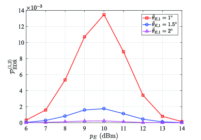
Refer to caption
(a) 𝒫EDR(1,2)superscriptsubscript𝒫EDR12\mathcal{P}_{\mathrm{EDR}}^{(1,2)} versus the transmit power of Eve.
Refer to caption
(b) 𝒫~EDR(2,2)superscriptsubscript~𝒫EDR22\tilde{\mathcal{P}}_{\mathrm{EDR}}^{(2,2)} and 𝒫EDR(2,2)superscriptsubscript𝒫EDR22\mathcal{P}_{\mathrm{EDR}}^{(2,2)} versus the transmit power of Eve.
Figure 3: EDRs under the PSA when there are only two effective channel observations.
Refer to caption
(a) CCDFs of d1(C)superscriptsubscript𝑑1𝐶d_{1}^{(C)},d1(N)superscriptsubscript𝑑1𝑁d_{1}^{(N)}, d^1subscript^𝑑1\hat{d}_{1}, dnsubscript𝑑𝑛d_{n}, and d^nsubscript^𝑑𝑛\hat{d}_{n}.
Refer to caption
(b) EDR versus K𝐾K under different transmit power of Eve.
Figure 4: EDRs under the PSA when there are more than two effective channel observations.

In Fig. 3 and Fig. 4, we evaluate the EDRs under the PSA through simulation. In Fig. 3, we simulate the case when there are only two effective channel observations, and in Fig. 4, we simulate the case when there are more than two effective channel observations. The reason why we simulate the two cases separately is that we use totally different methods to deal with these two cases as shown in Section III.

In Fig. 3, the number of antennas at the BS, the length of the PS, and the transmit power of the LU are set to M=64𝑀64M=64, τ=5𝜏5\tau=5, and pL=10dBmsubscript𝑝𝐿10dBmp_{L}=10~{}\mathrm{dBm} , respectively. We adopt the spatially correlated channel model introduced at the beginning of this section by setting TL=TE=1subscript𝑇𝐿subscript𝑇𝐸1T_{L}=T_{E}=1, θ¯L,1=0subscript¯𝜃𝐿1superscript0\bar{\theta}_{L,1}=0^{\circ}, and θL,1(D)=θE,1(D)=30superscriptsubscript𝜃𝐿1𝐷superscriptsubscript𝜃𝐸1𝐷superscript30\theta_{L,1}^{(D)}=\theta_{E,1}^{(D)}=30^{\circ}. In Fig. 3(a), we evaluate the EDRs under the condition that Eve only transmits one PS (K=1𝐾1K=1) but fails to hit the PS transmitted by the LU. As shown in Fig. 3(a), for fixed transmit power of Eve, when the direction of Eve gets closer to that of the LU, the EDR will significantly increase. This is because in this case, the statistical properties, e.g., the covariance matrix, of the legitimate and the illegitimate channels tend to be consistent, which makes it harder to differentiate the legitimate channel from the illegitimate channel. Besides, we show that the value of 𝒫EDR(1,2)superscriptsubscript𝒫EDR12\mathcal{P}_{\mathrm{EDR}}^{(1,2)} becomes large when pEsubscript𝑝𝐸p_{E} approaches to pLsubscript𝑝𝐿p_{L} and tends to be small when pEsubscript𝑝𝐸p_{E} is quite different from pEsubscript𝑝𝐸p_{E}. This is because if pEsubscript𝑝𝐸p_{E} is much smaller or much larger than pLsubscript𝑝𝐿p_{L}, the amplitude of 𝒚(E)superscript𝒚𝐸\bm{y}^{(E)} in (11) will be markedly distinct from that of 𝒚(L)superscript𝒚𝐿\bm{y}^{(L)}, which makes 𝒚(L)superscript𝒚𝐿\bm{y}^{(L)} more distinguishable and thus results in the decreasing EDRs. In Fig. 3(b), we evaluate the EDR under the condition that Eve transmits two PS (K=2𝐾2K=2) and successfully hits the PS transmitted by the LU. The performance of both the power comparison based method and the GLLR based method are checked. As we can see from Fig. 3(b), the GLLR based method generally outperforms the power comparison based method. This is due to the fact that in the power comparison based method, we only utilize partial information of the channel observations, i.e., the power, to determine 𝒚(L)superscript𝒚𝐿\bm{y}^{(L)}, while in the GLLR based method, high order statistics of 𝒚(L)superscript𝒚𝐿\bm{y}^{(L)} and 𝒚(E)superscript𝒚𝐸\bm{y}^{(E)}, i.e., the covariance matrices, are utilized to determine 𝒚(L)superscript𝒚𝐿\bm{y}^{(L)} and thus enjoys a lower EDR. Besides, we also observe that 𝒫EDR(2,2)superscriptsubscript𝒫EDR22\mathcal{P}_{\mathrm{EDR}}^{(2,2)} tends to increase with pEsubscript𝑝𝐸p_{E}. This is because when pEsubscript𝑝𝐸p_{E} becomes large, the statistics of 𝒚(L)superscript𝒚𝐿\bm{y}^{(L)} will be dominated by that of the term ejω(E)βPSA(2)𝒉Esuperscriptejsuperscript𝜔𝐸superscriptsubscript𝛽PSA2subscript𝒉𝐸\mathrm{e}^{\mathrm{j}\omega^{(E)}}\beta_{\mathrm{PSA}}^{(2)}\bm{h}_{E} in (18), and consequently, the impact of 𝒉Lsubscript𝒉𝐿\bm{h}_{L} on 𝒚(L)superscript𝒚𝐿\bm{y}^{(L)} becomes relatively smaller, which means that the statistical differences between 𝒚(L)superscript𝒚𝐿\bm{y}^{(L)} and 𝒚(E)superscript𝒚𝐸\bm{y}^{(E)} also gets relatively smaller. And therefore, it is harder to distinguish 𝒚(L)superscript𝒚𝐿\bm{y}^{(L)} from 𝒚(E)superscript𝒚𝐸\bm{y}^{(E)} when pEsubscript𝑝𝐸p_{E} is large.

In Fig. 4, we evaluate the EDRs when there are more than two effective channel observations. In the simulation, we set M=32𝑀32M=32, and other parameters are set to be the same as those in Fig. 3, unless specified. Note that the proposed distance based method does not utilize the statistical properties of the legitimate and illegitimate channels to identify 𝒚(L)superscript𝒚𝐿\bm{y}^{(L)}, and therefore, we set θ¯E,1=θ¯L,1=0subscript¯𝜃𝐸1subscript¯𝜃𝐿1superscript0\bar{\theta}_{E,1}=\bar{\theta}_{L,1}=0^{\circ} for simplicity. In Fig. 4(a), we keep βPSA(K)=0.5superscriptsubscript𝛽PSA𝐾0.5\beta_{\mathrm{PSA}}^{(K)}=0.5 regardless of the value of K𝐾K, and we plot the CCDFs of d1(C)superscriptsubscript𝑑1𝐶d_{1}^{(C)}, d1(N)superscriptsubscript𝑑1𝑁d_{1}^{(N)}, d^1subscript^𝑑1\hat{d}_{1}, dnsubscript𝑑𝑛d_{n}, and d~nsubscript~𝑑𝑛\tilde{d}_{n} to validate the effectiveness of the approximations in (29) and (33) and to provide a guideline on designing the decision threshold ϵitalic-ϵ\epsilon. As shown in Fig. 4(a), d~nsubscript~𝑑𝑛\tilde{d}_{n} approximates dnsubscript𝑑𝑛d_{n} very well and we can safely use the CCDF of d~nsubscript~𝑑𝑛\tilde{d}_{n}, i.e., 𝒫~F(ϵ)subscript~𝒫𝐹italic-ϵ\tilde{\mathcal{P}}_{F}\left(\epsilon\right), to approximate 𝒫F(ϵ)subscript𝒫𝐹italic-ϵ\mathcal{P}_{F}\left(\epsilon\right) as stated in Theorem 3. To determine a proper value of ϵitalic-ϵ\epsilon, we can choose those values of ϵitalic-ϵ\epsilon such that 𝒫{d~n>ϵ}𝒫subscript~𝑑𝑛italic-ϵ\mathcal{P}\{\tilde{d}_{n}>\epsilon\} is sufficiently small while 𝒫{d^1<ϵ}𝒫subscript^𝑑1italic-ϵ\mathcal{P}\{\hat{d}_{1}<\epsilon\} is close to 111. In this way, the EDR can be controlled to be small. In Fig. 4(b), we set τ=8𝜏8\tau=8, and we plot the EDRs against the numbers of PSs transmitted by Eve, i.e., K𝐾K, under different power budget of Eve. We choose ϵitalic-ϵ\epsilon such that 𝒫~F(ϵ)=103subscript~𝒫𝐹italic-ϵsuperscript103\tilde{\mathcal{P}}_{F}\left(\epsilon\right)=10^{-3}. As we can see from 4(b), with the proposed distance-based method, the BS can successfully identify 𝒚(L)superscript𝒚𝐿\bm{y}^{(L)} from the effective channel observation set while keeps the EDR to be generally small. We also observe that even if the Eve increases its power or transmits more PSs, the EDR appears to be robust and does not change with the transmission strategies of Eve.
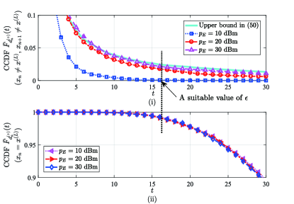
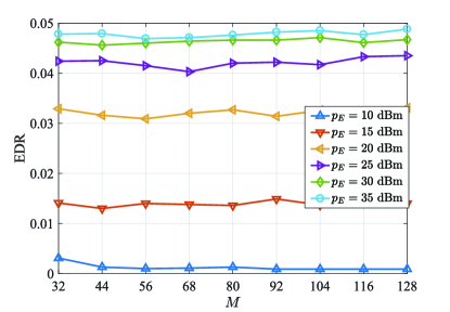
Refer to caption
(a) CCDF of dn(+)superscriptsubscript𝑑𝑛d_{n}^{(+)}.
Refer to caption
(b) EDR versus the number of antennas at BS.
Figure 5: EDRs under the PJA.

In Fig. 5, the EDRs under PJA are evaluated. In the simulation, the parameters are set to be the same as those in Fig. 4, unless specified. In Fig. 5(a), we set pL=15dBmsubscript𝑝𝐿15dBmp_{L}=15~{}\mathrm{dBm} and τ=5𝜏5\tau=5, and we plot the CCDFs of dn(+)superscriptsubscript𝑑𝑛d_{n}^{(+)} when 𝒙n𝒙(L)subscript𝒙𝑛superscript𝒙𝐿\bm{x}_{n}\neq\bm{x}^{(L)} and 𝒙n+1𝒙(L)subscript𝒙𝑛1superscript𝒙𝐿\bm{x}_{n+1}\neq\bm{x}^{(L)}, and when 𝒙n=𝒙(L)subscript𝒙𝑛superscript𝒙𝐿\bm{x}_{n}=\bm{x}^{(L)}, respectively, to provide a guideline on designing the decision threshold ϵitalic-ϵ\epsilon. As shown in Fig. 5(a), the analytical upper bound accurately approximates the simulation results if pEsubscript𝑝𝐸p_{E} is large. In this case, we can directly use 𝒫PJA(F)(ϵ)superscriptsubscript𝒫PJAFitalic-ϵ\mathcal{P}_{\mathrm{PJA}}^{(\mathrm{F})}\left(\epsilon\right) in (50) to design ϵitalic-ϵ\epsilon. When pEsubscript𝑝𝐸p_{E} is small, 𝒫PJA(F)(ϵ)superscriptsubscript𝒫PJAFitalic-ϵ\mathcal{P}_{\mathrm{PJA}}^{(\mathrm{F})}\left(\epsilon\right) becomes a strictly upper bound on the simulation results, and in this case, we do not need to restrict a small η𝜂\eta due to the gap between the upper bound and the exact value. In Fig. 5(b), we plot the EDRs versus the numbers of antennas at the BS under different transmit power of Eve. We set η=0.025𝜂0.025\eta=0.025 in the simulation. From Fig. 5(b), we observe that even though the EDR increases with transmit power of Eve, the EDR still keeps small when the power of the Eve becomes very high (lower than 0.050.050.05 when pE=35dBmsubscript𝑝𝐸35dBmp_{E}=35~{}\mathrm{dBm}), which validates the effectiveness of the proposed distance-based method.

We have to emphasize here that ensuring a small EDR is very important for the proposed downlink secure transmission scheme. This is because only when the BS successfully recognizes 𝒚(L)superscript𝒚𝐿\bm{y}^{(L)} can it estimates the channel of the LU. If a small EDR is not guaranteed, it is possible that the BS mistakes the illegitimate channel for the legitimate channel, which will undoubtedly result in the private information leakage to Eve.

VII-B Secrecy performance
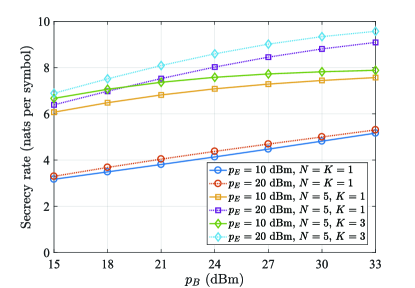
Refer to caption
(a) Secrecy rates versus the powers of BS.
Refer to caption
(b) Secrecy rates versus the powers of BS.
Figure 6: Secrecy performance under the PSA.

We have already shown that the BS can detect 𝒙(L)superscript𝒙𝐿\bm{x}^{(L)} with a low EDR in the previous subsection. In this subsection, we evaluate the secrecy performance in terms of secrecy rate under the proposed downlink secure transmission framework.

In Fig. 6, we plot the secrecy rates versus the downlink transmit powers of the BS when Eve carries out PSA. In the simulation, we set M=48𝑀48M=48, τ=5𝜏5\tau=5, pL=10dBmsubscript𝑝𝐿10dBmp_{L}=10~{}\mathrm{dBm}. The simulation results are obtained by averaging over 100010001000 random channel realizations. In each random trial, if the BS makes an error decision on 𝒚(L)superscript𝒚𝐿\bm{y}^{(L)}, we directly set the secrecy rate as 00. In Fig. 6(a), we set TL=TE=1subscript𝑇𝐿subscript𝑇𝐸1T_{L}=T_{E}=1, θ¯L,1=0subscript¯𝜃𝐿1superscript0\bar{\theta}_{L,1}=0^{\circ}, θ¯E,1=2subscript¯𝜃𝐸1superscript2\bar{\theta}_{E,1}=2^{\circ}, and θL,1(D)=θE,1(D)=30superscriptsubscript𝜃𝐿1𝐷superscriptsubscript𝜃𝐸1𝐷superscript30\theta_{L,1}^{(D)}=\theta_{E,1}^{(D)}=30^{\circ}. In Fig. 6(b), we set TL=TE=2subscript𝑇𝐿subscript𝑇𝐸2T_{L}=T_{E}=2, θL,1(D)=θE,1(D)=θL,2(D)=θE,2(D)=15superscriptsubscript𝜃𝐿1𝐷superscriptsubscript𝜃𝐸1𝐷superscriptsubscript𝜃𝐿2𝐷superscriptsubscript𝜃𝐸2𝐷superscript15\theta_{L,1}^{(D)}=\theta_{E,1}^{(D)}=\theta_{L,2}^{(D)}=\theta_{E,2}^{(D)}=15^{\circ}, and θ¯L,1=θ¯E,1=30subscript¯𝜃𝐿1subscript¯𝜃𝐸1superscript30\bar{\theta}_{L,1}=\bar{\theta}_{E,1}=30^{\circ}, and in each trial, θ¯L,2subscript¯𝜃𝐿2\bar{\theta}_{L,2} and θ¯E,2subscript¯𝜃𝐸2\bar{\theta}_{E,2} are independently and randomly generated within (5,5)superscript5superscript5\left(-5^{\circ},5^{\circ}\right). In Fig. 6, N=1𝑁1N=1 corresponds to the conventional training scheme wherein only one PS is allocated to the LU, and N=5𝑁5N=5 corresponds to the proposed training scheme wherein 555 PSs are simultaneously allocated to the LU. As we can see, compared to the conventional training scheme, allocating multiple PSs to the LU can greatly improve the secrecy rate. This is because when N=1𝑁1N=1, Eve can always hit the LU’s PS, which leads to a poor performance of channel estimation. However, when N>1𝑁1N>1, due to the fact that Eve does not know which PS the LU will transmit, it is possible for the BS to obtain uncontaminated channel observations of both the LU’s and Eve’s channels, which significantly improves the accuracy of the channel estimations, and thus the secrecy rate gets increased. Besides, we observe that the secrecy rate is improved when the transmit power of Eve is increased from 10dBm10dBm10~{}\mathrm{dBm} to 20dBm20dBm20~{}\mathrm{dBm}. Note that this phenomenon is totally different from that shown in [16]. In [16], the authors showed that without protection on the channel training procedure, Eve can always improve its wiretapping performance by increasing its power. However, with the proposed channel training scheme, if Eve increases its transmit power during the channel training procedure, the BS will obtain more accurate estimation of the illegitimate channel, which undoubtedly degrades the wiretapping capability of Eve.
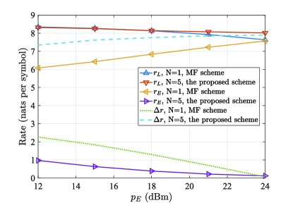
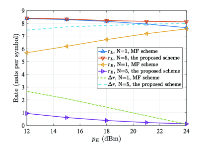
Refer to caption
(a) Achieve rates versus the powers of Eve.
Refer to caption
(b) Achieve rates versus the powers of Eve.
Figure 7: Secrecy performance under PJA.

In Fig. 7, we check the performance of the proposed secure downlink transmission framework under PJA. In the simulation, we set M=48𝑀48M=48, τ=5𝜏5\tau=5, pL=15subscript𝑝𝐿15p_{L}=15 (dBm), pB=20subscript𝑝𝐵20p_{B}=20 (dBm), and η=0.025𝜂0.025\eta=0.025. Besides, we consider an extreme terrible case for the LU where 𝑹L=𝑹Esubscript𝑹𝐿subscript𝑹𝐸\bm{R}_{L}=\bm{R}_{E}. In Fig. 7(a), the spatially correlated channel model is adopted by setting TL=TE=1subscript𝑇𝐿subscript𝑇𝐸1T_{L}=T_{E}=1, θ¯L,1=θ¯E,1=0subscript¯𝜃𝐿1subscript¯𝜃𝐸1superscript0\bar{\theta}_{L,1}=\bar{\theta}_{E,1}=0^{\circ}, and θL,1(D)=θE,1(D)=30superscriptsubscript𝜃𝐿1𝐷superscriptsubscript𝜃𝐸1𝐷superscript30\theta_{L,1}^{(D)}=\theta_{E,1}^{(D)}=30^{\circ}. In Fig. 7(b), we set 𝑹L=𝑹E=𝑰Msubscript𝑹𝐿subscript𝑹𝐸subscript𝑰𝑀\bm{R}_{L}=\bm{R}_{E}=\bm{I}_{M}. The achievable rates of the LU and Eve, denoted by rLln(1+SNRL)subscript𝑟𝐿1subscriptSNRLr_{L}\triangleq\ln(1+\mathrm{SNR_{L}}) and rEln(1+SNRE)subscript𝑟𝐸1subscriptSNREr_{E}\triangleq\ln(1+\mathrm{SNR_{E}}), respectively, and the differences of the achievable rates, denoted by ΔrrLrEsubscriptΔ𝑟subscript𝑟𝐿subscript𝑟𝐸\Delta_{r}\triangleq r_{L}-r_{E}, are used as the performance metrics. We also provide the performance of the conventional channel training (N=1𝑁1N=1) and matching filter (MF) beamforming data transmission scheme for comparison. The simulation results are obtained by averaging across 100010001000 random channel realizations. As we can see in Fig. 7, in the conventional channel training and MF beamforming transmission scheme, rEsubscript𝑟𝐸r_{E} is generally very high, and even approaches to rLsubscript𝑟𝐿r_{L} when pE=24dBmsubscript𝑝𝐸24dBmp_{E}=24~{}\mathrm{dBm}. This means that the data transmission suffers from serious signal leakage. The main reason accounts for this phenomenon is that under the condition 𝑹L=𝑹Esubscript𝑹𝐿subscript𝑹𝐸\bm{R}_{L}=\bm{R}_{E}, the BS can hardly distinguish the legitimate channel from the wiretap channel, and therefore, there is no way for the BS to restrain the signal leakage. However, in the proposed channel training and data transmission framework, rEsubscript𝑟𝐸r_{E} is always much lower than rLsubscript𝑟𝐿r_{L}, and even approaches to 00 when pE=24dBmsubscript𝑝𝐸24dBmp_{E}=24~{}\mathrm{dBm}. This is because with the proposed channel training scheme, the BS is able to simultaneously estimate the legitimate channel and the channel direction of the wiretap channel, based on which zero-forcing beamforming can be utilized to greatly reduce the signal power received by Eve. We also observe that rLsubscript𝑟𝐿r_{L} slightly decreases with the increase of pEsubscript𝑝𝐸p_{E}. This is because when pEsubscript𝑝𝐸p_{E} gets large, the EDR also increase as shown in Fig. 5(b). This means that the probability that the BS mistakes the illegitimate channel as the legitimate channel increases, and therefore rLsubscript𝑟𝐿r_{L} decreases accordingly.

VIII Conclusion

In this paper, a framework, including the RCT scheme and the SB vector design, was proposed to combat with the PSA and PJA during the channel training phase in a TDD system. We hid LU’s PS by letting the LU randomly select a PS to transmit. The BS can recognize LU’s PS by utilizing the different channel statistics between Eve and the LU. It was shown that though the BS does not know which PS will be transmitted by LU in advance, it can correctly recognize it with very high probability, even the channel statistics of Eve is very similar to that of the LU. We showed that the secrecy rate is remarkably increased when the proposed framework is utilized.

At last, we have to point out that in this paper, we only investigated the single-cell systems. When it comes to multi-cell systems, the PSs will be reused in multiple cells, and the pilot contamination from the other cells will makes the problem much more difficult and complicated. To combat PSA and PJA in multi-cell situations will be one of our future works.

-A The Proof of Theorem 2

Define a unitary matrix 𝚲(x)diag(𝑰M,ejx𝑰M)𝚲𝑥diagsubscript𝑰𝑀superscriptej𝑥subscript𝑰𝑀\bm{\Lambda}\left(x\right)\triangleq\mathrm{diag}\left(\bm{I}_{M},\mathrm{e}^{\mathrm{j}x}\bm{I}_{M}\right). Because 𝒉Esubscript𝒉𝐸\bm{h}_{E} is circular and symmetrical, we have 𝒫~EDR(2,2)=𝒫{𝒈~12𝒈~22<0}superscriptsubscript~𝒫EDR22𝒫superscriptnormsubscript~𝒈12superscriptnormsubscript~𝒈220\tilde{\mathcal{P}}_{\mathrm{EDR}}^{(2,2)}=\mathcal{P}\left\{\left\|\tilde{\bm{g}}_{1}\right\|^{2}-\left\|\tilde{\bm{g}}_{2}\right\|^{2}<0\right\}, where 𝒈~1𝒉L+βPSA(2)𝒉E+𝒛(L)subscript~𝒈1subscript𝒉𝐿superscriptsubscript𝛽PSA2subscript𝒉𝐸superscript𝒛𝐿\tilde{\bm{g}}_{1}\triangleq\bm{h}_{L}+\beta_{\mathrm{PSA}}^{(2)}\bm{h}_{E}+\bm{z}^{(L)}, 𝒈~2ejω~βPSA(2)𝒉E+𝒛(E)subscript~𝒈2superscriptej~𝜔superscriptsubscript𝛽PSA2subscript𝒉𝐸superscript𝒛𝐸\tilde{\bm{g}}_{2}\triangleq\mathrm{e}^{\mathrm{j}\tilde{\omega}}\beta_{\mathrm{PSA}}^{(2)}\bm{h}_{E}+\bm{z}^{(E)}, and ω~ω(E)ω(L)~𝜔superscript𝜔𝐸superscript𝜔𝐿\tilde{\omega}\triangleq\omega^{(E)}-\omega^{(L)}. Using 𝚲(x)𝚲𝑥\bm{\Lambda}\left(x\right), we have 𝒫~EDR(2,2)=𝒫{𝒈~H𝚲(π)𝒈~<0}superscriptsubscript~𝒫EDR22𝒫superscript~𝒈𝐻𝚲𝜋~𝒈0\tilde{\mathcal{P}}_{\mathrm{EDR}}^{(2,2)}=\mathcal{P}\left\{\tilde{\bm{g}}^{H}\bm{\Lambda}\left(\pi\right)\tilde{\bm{g}}<0\right\}, where 𝒈~[𝒈~1H,𝒈~2H]H(𝟎,𝑹g(ω~))similar-tosubscript~𝒈superscriptsuperscriptsubscript~𝒈1𝐻superscriptsubscript~𝒈2𝐻𝐻0subscript𝑹𝑔~𝜔\tilde{\bm{g}}_{\triangleq}\left[\tilde{\bm{g}}_{1}^{H},\tilde{\bm{g}}_{2}^{H}\right]^{H}\sim\mathbb{CN}\left(\bm{0},\bm{R}_{g}\left(\tilde{\omega}\right)\right) with

𝑹g(ω~)subscript𝑹𝑔~𝜔\displaystyle\bm{R}_{g}\left(\tilde{\omega}\right) 𝔼(𝒈~𝒈~H)=[𝑹L,E,z(2)ejω~𝑹E(2)ejω~𝑹E(2)𝑹E,z(2)]absent𝔼~𝒈superscript~𝒈𝐻matrixsuperscriptsubscript𝑹𝐿𝐸𝑧2superscriptej~𝜔superscriptsubscript𝑹𝐸2superscriptej~𝜔superscriptsubscript𝑹𝐸2superscriptsubscript𝑹𝐸𝑧2\displaystyle\triangleq\mathbb{E}\left(\tilde{\bm{g}}\tilde{\bm{g}}^{H}\right)=\begin{bmatrix}\bm{R}_{L,E,z}^{(2)}&\mathrm{e}^{-\mathrm{j}\tilde{\omega}}\bm{R}_{E}^{(2)}\\ \mathrm{e}^{\mathrm{j}\tilde{\omega}}\bm{R}_{E}^{(2)}&\bm{R}_{E,z}^{(2)}\end{bmatrix}
=𝚲(ω~)𝑹g(0)𝚲(ω~).absent𝚲~𝜔subscript𝑹𝑔0𝚲~𝜔\displaystyle=\bm{\Lambda}\left(\tilde{\omega}\right)\bm{R}_{g}\left(0\right)\bm{\Lambda}\left(-\tilde{\omega}\right). (53)

Therefore, we further have

𝒫~EDR(2,2)superscriptsubscript~𝒫EDR22\displaystyle\tilde{\mathcal{P}}_{\mathrm{EDR}}^{(2,2)} =𝒫{𝒈~H(𝑹g(ω~))12(𝑹g(ω~))12𝚲(π)\displaystyle=\mathcal{P}\Big{\{}\tilde{\bm{g}}^{H}\left(\bm{R}_{g}\left(\tilde{\omega}\right)\right)^{-\frac{1}{2}}\left(\bm{R}_{g}\left(\tilde{\omega}\right)\right)^{\frac{1}{2}}\bm{\Lambda}\left(\pi\right)
×(𝑹g(ω~))12(𝑹g(ω~))12𝒈~<0}\displaystyle\quad\quad\quad\times\left(\bm{R}_{g}\left(\tilde{\omega}\right)\right)^{\frac{1}{2}}\left(\bm{R}_{g}\left(\tilde{\omega}\right)\right)^{-\frac{1}{2}}\tilde{\bm{g}}<0\Big{\}}
=𝒫{𝒈~H𝚲(ω~)(𝑹g(0))12(𝑹g(0))12𝚲(π)\displaystyle=\mathcal{P}\Big{\{}\tilde{\bm{g}}^{H}\bm{\Lambda}\left(\tilde{\omega}\right)\left(\bm{R}_{g}\left(0\right)\right)^{-\frac{1}{2}}\left(\bm{R}_{g}\left(0\right)\right)^{\frac{1}{2}}\bm{\Lambda}\left(\pi\right)
×(𝑹g(0))12(𝑹g(0))12𝚲(ω~)𝒈~<0}\displaystyle\quad\quad\quad\times\left(\bm{R}_{g}\left(0\right)\right)^{\frac{1}{2}}\left(\bm{R}_{g}\left(0\right)\right)^{-\frac{1}{2}}\bm{\Lambda}\left(-\tilde{\omega}\right)\tilde{\bm{g}}<0\Big{\}}
=𝒫{𝜶H𝑾𝜶<0},absent𝒫superscript𝜶𝐻𝑾𝜶0\displaystyle=\mathcal{P}\left\{\bm{\alpha}^{H}\bm{W}\bm{\alpha}<0\right\}, (54)

where 𝜶(𝑹g(0))12𝚲(ω~)𝒈~𝜶superscriptsubscript𝑹𝑔012𝚲~𝜔~𝒈\bm{\alpha}\triangleq\left(\bm{R}_{g}\left(0\right)\right)^{-\frac{1}{2}}\bm{\Lambda}\left(-\tilde{\omega}\right)\tilde{\bm{g}} and 𝑾(𝑹g(0))12𝚲(π)(𝑹g(0))12𝑾superscriptsubscript𝑹𝑔012𝚲𝜋superscriptsubscript𝑹𝑔012\bm{W}\triangleq\left(\bm{R}_{g}\left(0\right)\right)^{\frac{1}{2}}\bm{\Lambda}\left(\pi\right)\left(\bm{R}_{g}\left(0\right)\right)^{\frac{1}{2}}. Note that 𝑾𝑾\bm{W} does not depend on ω𝜔\omega. As for 𝜶𝜶\bm{\alpha}, it can be easily checked that 𝔼{𝜶𝜶H}=𝑰2M𝔼𝜶superscript𝜶𝐻subscript𝑰2𝑀\mathbb{E}\left\{\bm{\alpha}\bm{\alpha}^{H}\right\}=\boldsymbol{I}_{2M}.

-B The proof Lemma 1

We first show that 𝔼X,Y{ln(1+X1+Y)}subscript𝔼𝑋𝑌1𝑋1𝑌\mathbb{E}_{X,Y}\left\{\ln\left(\frac{1+X}{1+Y}\right)\right\} and ln(1+𝔼X{X}1+𝔼Y{Y})1subscript𝔼𝑋𝑋1subscript𝔼𝑌𝑌\ln\left(\frac{1+\mathbb{E}_{X}\left\{X\right\}}{1+\mathbb{E}_{Y}\left\{Y\right\}}\right) have a common lower bound as follows,

𝔼X,Y{ln(1+X1+Y)}subscript𝔼𝑋𝑌1𝑋1𝑌\displaystyle\mathbb{E}_{X,Y}\left\{\ln\left(\frac{1+X}{1+Y}\right)\right\}
(a)ln(1+1𝔼X{1/X})ln(1+𝔼Y{Y})𝑎11subscript𝔼𝑋1𝑋1subscript𝔼𝑌𝑌\displaystyle\overset{(a)}{\geq}\ln\left(1+\frac{1}{\mathbb{E}_{X}\left\{1/X\right\}}\right)-\ln\left(1+\mathbb{E}_{Y}\left\{Y\right\}\right)
(b)ln(1+𝔼X{X}1+𝔼Y{Y}),𝑏1subscript𝔼𝑋𝑋1subscript𝔼𝑌𝑌\displaystyle\overset{(b)}{\leq}\ln\left(\frac{1+\mathbb{E}_{X}\left\{X\right\}}{1+\mathbb{E}_{Y}\left\{Y\right\}}\right), (55)

where step (a)𝑎(a) is obtained by applying Jensen’s inequality to convex functions ln(1+1x)11𝑥\ln\left(1+\frac{1}{x}\right) and ln(11+x)11𝑥\ln\left(\frac{1}{1+x}\right), and step (b)𝑏(b) is because 𝔼X{1X}1𝔼X{X}subscript𝔼𝑋1𝑋1subscript𝔼𝑋𝑋\mathbb{E}_{X}\left\{\frac{1}{X}\right\}\geq\frac{1}{\mathbb{E}_{X}\left\{X\right\}}. Now we show that 𝔼X,Y{ln(1+X1+Y)}subscript𝔼𝑋𝑌1𝑋1𝑌\mathbb{E}_{X,Y}\left\{\ln\left(\frac{1+X}{1+Y}\right)\right\} and ln(1+𝔼X{X}1+𝔼Y{Y})1subscript𝔼𝑋𝑋1subscript𝔼𝑌𝑌\ln\left(\frac{1+\mathbb{E}_{X}\left\{X\right\}}{1+\mathbb{E}_{Y}\left\{Y\right\}}\right) have a common upper bound as follows,

𝔼X,Y{ln(1+X1+Y)}subscript𝔼𝑋𝑌1𝑋1𝑌\displaystyle\mathbb{E}_{X,Y}\left\{\ln\left(\frac{1+X}{1+Y}\right)\right\}
(a)ln(1+𝔼X{X})ln(1+1𝔼Y{1/Y})𝑎1subscript𝔼𝑋𝑋11subscript𝔼𝑌1𝑌\displaystyle\overset{(a)}{\leq}\ln\left(1+\mathbb{E}_{X}\left\{X\right\}\right)-\ln\left(1+\frac{1}{\mathbb{E}_{Y}\left\{1/Y\right\}}\right)
(b)ln(1+𝔼X{X}1+𝔼Y{Y}),𝑏1subscript𝔼𝑋𝑋1subscript𝔼𝑌𝑌\displaystyle\overset{(b)}{\geq}\ln\left(\frac{1+\mathbb{E}_{X}\left\{X\right\}}{1+\mathbb{E}_{Y}\left\{Y\right\}}\right), (56)

where step (a)𝑎(a) is due to the fact that ln(1+x)1𝑥\ln\left(1+x\right) and ln(1+1x)11𝑥-\ln\left(1+\frac{1}{x}\right) are concave functions, and step (b)𝑏(b) is because 𝔼Y{1Y}1𝔼Y{Y}subscript𝔼𝑌1𝑌1subscript𝔼𝑌𝑌\mathbb{E}_{Y}\left\{\frac{1}{Y}\right\}\geq\frac{1}{\mathbb{E}_{Y}\left\{Y\right\}}. As we can see, 𝔼X,Y{ln(1+X1+Y)}subscript𝔼𝑋𝑌1𝑋1𝑌\mathbb{E}_{X,Y}\left\{\ln\left(\frac{1+X}{1+Y}\right)\right\} and ln(1+𝔼X{X}1+𝔼Y{Y})1subscript𝔼𝑋𝑋1subscript𝔼𝑌𝑌\ln\left(\frac{1+\mathbb{E}_{X}\left\{X\right\}}{1+\mathbb{E}_{Y}\left\{Y\right\}}\right) has the same upper and lower bound, and thus we can use ln(1+𝔼X{X}1+𝔼Y{Y})1subscript𝔼𝑋𝑋1subscript𝔼𝑌𝑌\ln\left(\frac{1+\mathbb{E}_{X}\left\{X\right\}}{1+\mathbb{E}_{Y}\left\{Y\right\}}\right) to approximate 𝔼X,Y{ln(1+X1+Y)}subscript𝔼𝑋𝑌1𝑋1𝑌\mathbb{E}_{X,Y}\left\{\ln\left(\frac{1+X}{1+Y}\right)\right\}.

-C Proof of Theorem 5

The derivation of Theorem 5 is given as follows,

𝒫{dPJA,n(+)>ϵ}𝒫superscriptsubscript𝑑PJA𝑛italic-ϵ\displaystyle\mathcal{P}\left\{d_{\mathrm{PJA},n}^{(+)}>\epsilon\right\}
=𝒫{minaμnβPJA𝒉E+𝒛n\displaystyle=\mathcal{P}\Big{\{}\mathop{\mathrm{min}}\limits_{a}~{}\|\mu_{n}\beta_{\mathrm{PJA}}\bm{h}_{E}+\bm{z}_{n}
a(μn+1βPJA𝒉E+𝒛n+1)2>ϵ}\displaystyle\quad-a\left(\mu_{n+1}\beta_{\mathrm{PJA}}\bm{h}_{E}+\bm{z}_{n+1}\right)\|^{2}>\epsilon\Big{\}}
(a)𝒫{𝒛nμn𝒛n+1/μn+12>ϵ}𝑎𝒫superscriptnormsubscript𝒛𝑛subscript𝜇𝑛subscript𝒛𝑛1subscript𝜇𝑛12italic-ϵ\displaystyle\overset{(a)}{\leq}\mathcal{P}\left\{\left\|\bm{z}_{n}-\mu_{n}\bm{z}_{n+1}/\mu_{n+1}\right\|^{2}>\epsilon\right\}
=(b)τ20+0+eτ(x+y)Γ(M,ϵxσz2(x+y))Γ(M)dxdy𝑏superscript𝜏2superscriptsubscript0superscriptsubscript0superscripte𝜏𝑥𝑦Γ𝑀italic-ϵ𝑥superscriptsubscript𝜎𝑧2𝑥𝑦Γ𝑀differential-d𝑥differential-d𝑦\displaystyle\overset{(b)}{=}\tau^{2}\int_{0}^{+\infty}\int_{0}^{+\infty}\mathrm{e}^{-\tau\left(x+y\right)}\frac{\Gamma\left(M,\frac{\epsilon x}{\sigma_{z}^{2}\left(x+y\right)}\right)}{\Gamma\left(M\right)}\mathrm{d}x\mathrm{d}y
=(c)τ20+v+eτuΓ(M,ϵvσz2u)Γ(M)dudv𝑐superscript𝜏2superscriptsubscript0superscriptsubscript𝑣superscripte𝜏𝑢Γ𝑀italic-ϵ𝑣superscriptsubscript𝜎𝑧2𝑢Γ𝑀differential-d𝑢differential-d𝑣\displaystyle\overset{(c)}{=}\tau^{2}\int_{0}^{+\infty}\int_{v}^{+\infty}\mathrm{e}^{-\tau u}\frac{\Gamma\left(M,\frac{\epsilon v}{\sigma_{z}^{2}u}\right)}{\Gamma\left(M\right)}\mathrm{d}u\mathrm{d}v
=(d)τ20+0ueτueϵσz2uvm=0M1(ϵσz2u)mvmm!dvdu𝑑superscript𝜏2superscriptsubscript0superscriptsubscript0𝑢superscripte𝜏𝑢superscripteitalic-ϵsuperscriptsubscript𝜎𝑧2𝑢𝑣superscriptsubscript𝑚0𝑀1superscriptitalic-ϵsuperscriptsubscript𝜎𝑧2𝑢𝑚superscript𝑣𝑚𝑚d𝑣d𝑢\displaystyle\overset{(d)}{=}\tau^{2}\int_{0}^{+\infty}\int_{0}^{u}\mathrm{e}^{-\tau u}\mathrm{e}^{-\frac{\epsilon}{\sigma_{z}^{2}u}v}\sum_{m=0}^{M-1}\frac{\left(\frac{\epsilon}{\sigma_{z}^{2}u}\right)^{m}v^{m}}{m!}\mathrm{d}v\mathrm{d}u
=(e)τ20+eτum=0M1{σz2uϵk=0muk(ϵσz2u)k1eϵσz2k!}du𝑒superscript𝜏2superscriptsubscript0superscripte𝜏𝑢superscriptsubscript𝑚0𝑀1superscriptsubscript𝜎𝑧2𝑢italic-ϵsuperscriptsubscript𝑘0𝑚superscript𝑢𝑘superscriptitalic-ϵsuperscriptsubscript𝜎𝑧2𝑢𝑘1superscripteitalic-ϵsuperscriptsubscript𝜎𝑧2𝑘d𝑢\displaystyle\overset{(e)}{=}\tau^{2}\int_{0}^{+\infty}\mathrm{e}^{-\tau u}\sum_{m=0}^{M-1}\left\{\frac{\sigma_{z}^{2}u}{\epsilon}-\sum_{k=0}^{m}\frac{u^{k}\left(\frac{\epsilon}{\sigma_{z}^{2}u}\right)^{k-1}}{\mathrm{e}^{\frac{\epsilon}{\sigma_{z}^{2}}}k!}\right\}\mathrm{d}u
=σz2Mϵm=0M1k=0m(ϵσz2)k1eϵσz2k!.absentsuperscriptsubscript𝜎𝑧2𝑀italic-ϵsuperscriptsubscript𝑚0𝑀1superscriptsubscript𝑘0𝑚superscriptitalic-ϵsuperscriptsubscript𝜎𝑧2𝑘1superscripteitalic-ϵsuperscriptsubscript𝜎𝑧2𝑘\displaystyle=\frac{\sigma_{z}^{2}M}{\epsilon}-\sum_{m=0}^{M-1}\sum_{k=0}^{m}\frac{\left(\frac{\epsilon}{\sigma_{z}^{2}}\right)^{k-1}}{\mathrm{e}^{\frac{\epsilon}{\sigma_{z}^{2}}}k!}. (57)

In (57), step (a)𝑎(a) is obtained by setting a=μnμn+1𝑎subscript𝜇𝑛subscript𝜇𝑛1a=\frac{\mu_{n}}{\mu_{n+1}}, step (b)𝑏(b) is because 𝒛nμn𝒛n+1/μn+12𝔾(M,|μn+1|2+|μn|2|μn+1|2)similar-tosuperscriptnormsubscript𝒛𝑛subscript𝜇𝑛subscript𝒛𝑛1subscript𝜇𝑛12𝔾𝑀superscriptsubscript𝜇𝑛12superscriptsubscript𝜇𝑛2superscriptsubscript𝜇𝑛12\left\|\bm{z}_{n}-\mu_{n}\bm{z}_{n+1}/\mu_{n+1}\right\|^{2}\sim\mathbb{G}\left(M,\frac{\left|\mu_{n+1}\right|^{2}+\left|\mu_{n}\right|^{2}}{\left|\mu_{n+1}\right|^{2}}\right) when μnsubscript𝜇𝑛\mu_{n} and μn+1subscript𝜇𝑛1\mu_{n+1} are fixed, and |μn|2𝔼(1τ)similar-tosuperscriptsubscript𝜇𝑛2𝔼1𝜏\left|\mu_{n}\right|^{2}\sim\mathbb{E}\left(\frac{1}{\tau}\right) and |μn+1|2𝔼(1τ)similar-tosuperscriptsubscript𝜇𝑛12𝔼1𝜏\left|\mu_{n+1}\right|^{2}\sim\mathbb{E}\left(\frac{1}{\tau}\right), step (c)𝑐(c) is obtained by x+yu𝑥𝑦𝑢x+y\rightarrow u and xv𝑥𝑣x\rightarrow v, step (d)𝑑(d) is obtained by using [38, Eq. (3.3512)], and step (e)𝑒(e) is obtained by using [38, Eq. (3.3511)].

-D CCDF of quadratic formula of Gaussian random vector

We provide an expression for 𝒫{𝒙H𝛀𝒙>t}𝒫superscript𝒙𝐻𝛀𝒙𝑡\mathcal{P}\left\{\bm{x}^{H}\bm{\Omega}\bm{x}>t\right\} in this appendix, where t0𝑡0t\geq 0, 𝒙(𝟎,𝑰L)similar-to𝒙0subscript𝑰𝐿\bm{x}\sim\mathbb{CN}\left(\bm{0},\bm{I}_{L}\right), and 𝛀L×L𝛀superscript𝐿𝐿\bm{\Omega}\in\mathbb{C}^{L\times L} is an indefinite Hermitian matrix. Denote s(1,1)<s(1,2)<<s(1,n1)superscript𝑠11superscript𝑠12superscript𝑠1subscript𝑛1s^{(1,1)}<s^{(1,2)}<\cdots<s^{(1,n_{1})} as the n1subscript𝑛1n_{1} distinct positive eigenvalues of 𝛀𝛀\bm{\Omega} with algebraic multiplicities given by m1,1,m1,2,,m1,n1subscript𝑚11subscript𝑚12subscript𝑚1subscript𝑛1m_{1,1},m_{1,2},\cdots,m_{1,n_{1}}, respectively. Denote s(2,n2)<s(2,n21)<<s(2,1)superscript𝑠2subscript𝑛2superscript𝑠2subscript𝑛21superscript𝑠21s^{(2,n_{2})}<s^{(2,n_{2}-1)}<\cdots<s^{(2,1)} as the n2subscript𝑛2n_{2} distinct negative eigenvalues of 𝛀𝛀\bm{\Omega} with algebraic multiplicities given by m2,n2,m2,n21,,m2,1subscript𝑚2subscript𝑛2subscript𝑚2subscript𝑛21subscript𝑚21m_{2,n_{2}},m_{2,n_{2}-1},\cdots,m_{2,1}, respectively. We have

𝒫{𝒙H𝛀𝒙t}𝒫superscript𝒙𝐻𝛀𝒙𝑡\displaystyle\mathcal{P}\left\{\bm{x}^{H}\bm{\Omega}\bm{x}\geq t\right\} =𝒫{𝒙H𝑼𝑫𝑼H𝒙t}absent𝒫superscript𝒙𝐻𝑼𝑫superscript𝑼𝐻𝒙𝑡\displaystyle=\mathcal{P}\left\{\bm{x}^{H}\bm{U}\bm{D}\bm{U}^{H}\bm{x}\geq t\right\}
=𝒫{𝝁H𝑫𝝁t}absent𝒫superscript𝝁𝐻𝑫𝝁𝑡\displaystyle=\mathcal{P}\left\{\bm{\mu}^{H}\bm{D}\bm{\mu}\geq t\right\}
=𝒫{Q1Q2t}absent𝒫subscript𝑄1subscript𝑄2𝑡\displaystyle=\mathcal{P}\left\{Q_{1}-Q_{2}\geq t\right\}
=0+y+t+fQ1(x)fQ2(y)dxdy,absentsuperscriptsubscript0superscriptsubscript𝑦𝑡subscript𝑓subscript𝑄1𝑥subscript𝑓subscript𝑄2𝑦differential-d𝑥differential-d𝑦\displaystyle=\int_{0}^{+\infty}\int_{y+t}^{+\infty}f_{Q_{1}}\left(x\right)f_{Q_{2}}\left(y\right)\mathrm{d}x\mathrm{d}y,

where 𝑼𝑫𝑼H=𝛀𝑼𝑫superscript𝑼𝐻𝛀\bm{U}\bm{D}\bm{U}^{H}=\bm{\Omega} is the eigenvalue decomposition, and

𝝁𝝁\displaystyle\bm{\mu} 𝑼H𝒙(𝟎,𝑰L),absentsuperscript𝑼𝐻𝒙similar-to0subscript𝑰𝐿\displaystyle\triangleq\bm{U}^{H}\bm{x}\sim\mathbb{CN}\left(\bm{0},\bm{I}_{L}\right),
Q1subscript𝑄1\displaystyle Q_{1} i=1n1G1,i,Q2j=1n2G2,j,formulae-sequenceabsentsuperscriptsubscript𝑖1subscript𝑛1subscript𝐺1𝑖subscript𝑄2superscriptsubscript𝑗1subscript𝑛2subscript𝐺2𝑗\displaystyle\triangleq\sum_{i=1}^{n_{1}}G_{1,i},\quad Q_{2}\triangleq\sum_{j=1}^{n_{2}}G_{2,j},
G1,isubscript𝐺1𝑖\displaystyle G_{1,i} 𝔾1,i(m1,i,s(1,i)),i=1,2,,n1,formulae-sequencesimilar-toabsentsubscript𝔾1𝑖subscript𝑚1𝑖superscript𝑠1𝑖𝑖12subscript𝑛1\displaystyle\sim\mathbb{G}_{1,i}\left(m_{1,i},s^{(1,i)}\right),i=1,2,\cdots,n_{1},
G2,jsubscript𝐺2𝑗\displaystyle G_{2,j} 𝔾2,j(m2,j,|s(2,i)|),j=1,2,,n2.formulae-sequencesimilar-toabsentsubscript𝔾2𝑗subscript𝑚2𝑗superscript𝑠2𝑖𝑗12subscript𝑛2\displaystyle\sim\mathbb{G}_{2,j}\left(m_{2,j},\left|s^{(2,i)}\right|\right),j=1,2,\cdots,n_{2}.

According to [36], the PDF of Qqsubscript𝑄𝑞Q_{q}, for q{1,2}𝑞12q\in\{1,2\}, can be written as

fQq(x)=𝕀{x>0}k=0δ¯q,kxρq+k1|s(q,1)|ρq+kΓ(ρq+k)ex|s(q,1)|,subscript𝑓subscript𝑄𝑞𝑥subscript𝕀𝑥0superscriptsubscript𝑘0subscript¯𝛿𝑞𝑘superscript𝑥subscript𝜌𝑞𝑘1superscriptsuperscript𝑠𝑞1subscript𝜌𝑞𝑘Γsubscript𝜌𝑞𝑘superscripte𝑥superscript𝑠𝑞1\displaystyle f_{Q_{q}}\left(x\right)=\mathbb{I}_{\{x>0\}}\sum_{k=0}^{\infty}\frac{\bar{\delta}_{q,k}x^{\rho_{q}+k-1}}{\left|s^{(q,1)}\right|^{\rho_{q}+k}\Gamma\left(\rho_{q}+k\right)}\mathrm{e}^{-\frac{x}{\left|s^{(q,1)}\right|}},

where for q{1,2}𝑞12q\in\{1,2\}, δ¯q,kCqδq,ksubscript¯𝛿𝑞𝑘subscript𝐶𝑞subscript𝛿𝑞𝑘\bar{\delta}_{q,k}\triangleq C_{q}\delta_{q,k}, Cqi=1nq(s(q,1)s(q,i))mq,isubscript𝐶𝑞superscriptsubscriptproduct𝑖1subscript𝑛𝑞superscriptsuperscript𝑠𝑞1superscript𝑠𝑞𝑖subscript𝑚𝑞𝑖C_{q}\triangleq\prod_{i=1}^{n_{q}}\left(\frac{s^{(q,1)}}{s^{(q,i)}}\right)^{m_{q,i}}, δq,k+11k+1i=1k+1iγq,iδq,k+1isubscript𝛿𝑞𝑘11𝑘1superscriptsubscript𝑖1𝑘1𝑖subscript𝛾𝑞𝑖subscript𝛿𝑞𝑘1𝑖\delta_{q,k+1}\triangleq\frac{1}{k+1}\sum_{i=1}^{k+1}i\gamma_{q,i}\delta_{q,k+1-i}, δq,01subscript𝛿𝑞01\delta_{q,0}\triangleq 1, γq,ki=1nqmq,ik(1s(q,1)s(q,i))ksubscript𝛾𝑞𝑘superscriptsubscript𝑖1subscript𝑛𝑞subscript𝑚𝑞𝑖𝑘superscript1superscript𝑠𝑞1superscript𝑠𝑞𝑖𝑘\gamma_{q,k}\triangleq\sum_{i=1}^{n_{q}}\frac{m_{q,i}}{k}\left(1-\frac{s^{(q,1)}}{s^{(q,i)}}\right)^{k}, and ρqi=1nqmq,isubscript𝜌𝑞superscriptsubscript𝑖1subscript𝑛𝑞subscript𝑚𝑞𝑖\rho_{q}\triangleq\sum_{i=1}^{n_{q}}m_{q,i}. Based on fQq(x)subscript𝑓subscript𝑄𝑞𝑥f_{Q_{q}}\left(x\right), we have

0+y+t+fQ1(x)fQ2(y)dxdysuperscriptsubscript0superscriptsubscript𝑦𝑡subscript𝑓subscript𝑄1𝑥subscript𝑓subscript𝑄2𝑦differential-d𝑥differential-d𝑦\displaystyle\int_{0}^{+\infty}\int_{y+t}^{+\infty}f_{Q_{1}}\left(x\right)f_{Q_{2}}\left(y\right)\mathrm{d}x\mathrm{d}y
=0+k2=0δ¯2,k2yρ2+k21ey|s(2,1)||s(2,1)|ρ2+k2Γ(ρ2+k2)absentsuperscriptsubscript0superscriptsubscriptsubscript𝑘20subscript¯𝛿2subscript𝑘2superscript𝑦subscript𝜌2subscript𝑘21superscripte𝑦superscript𝑠21superscriptsuperscript𝑠21subscript𝜌2subscript𝑘2Γsubscript𝜌2subscript𝑘2\displaystyle=\int_{0}^{+\infty}\sum_{k_{2}=0}^{\infty}\frac{\bar{\delta}_{2,k_{2}}y^{\rho_{2}+k_{2}-1}\mathrm{e}^{-\frac{y}{\left|s^{(2,1)}\right|}}}{\left|s^{(2,1)}\right|^{\rho_{2}+k_{2}}\Gamma\left(\rho_{2}+k_{2}\right)}
×y+t+k1=0δ¯1,k1xρ1+k11ex|s(1,1)||s(1,1)|ρ1+k1Γ(ρ1+k1)dxdy\displaystyle\quad\times\int_{y+t}^{+\infty}\sum_{k_{1}=0}^{\infty}\frac{\bar{\delta}_{1,k_{1}}x^{\rho_{1}+k_{1}-1}\mathrm{e}^{-\frac{x}{\left|s^{(1,1)}\right|}}}{\left|s^{(1,1)}\right|^{\rho_{1}+k_{1}}\Gamma\left(\rho_{1}+k_{1}\right)}\mathrm{d}x\mathrm{d}y
=k1=0k2=0δ¯1,k1δ¯1,k2Δk1,k2(t).absentsuperscriptsubscriptsubscript𝑘10superscriptsubscriptsubscript𝑘20subscript¯𝛿1subscript𝑘1subscript¯𝛿1subscript𝑘2subscriptΔsubscript𝑘1subscript𝑘2𝑡\displaystyle=\sum_{k_{1}=0}^{\infty}\sum_{k_{2}=0}^{\infty}\bar{\delta}_{1,k_{1}}\bar{\delta}_{1,k_{2}}\Delta_{k_{1},k_{2}}\left(t\right). (58)

where due to the fact that ρ1subscript𝜌1\rho_{1} and ρ2subscript𝜌2\rho_{2} are integers, Δk1,k2(t)subscriptΔsubscript𝑘1subscript𝑘2𝑡\Delta_{k_{1},k_{2}}\left(t\right) can be written as (59) at the top of the next page.

Δk1,k2(t)subscriptΔsubscript𝑘1subscript𝑘2𝑡\displaystyle\Delta_{k_{1},k_{2}}\left(t\right) =0+yρ2+k21eyΓ(ρ1+k1,|s(2,1)s(1,1)|(y+t|s(2,1)|))Γ(ρ2+k2)Γ(ρ1+k1)dyabsentsuperscriptsubscript0superscript𝑦subscript𝜌2subscript𝑘21superscripte𝑦Γsubscript𝜌1subscript𝑘1superscript𝑠21superscript𝑠11𝑦𝑡superscript𝑠21Γsubscript𝜌2subscript𝑘2Γsubscript𝜌1subscript𝑘1differential-d𝑦\displaystyle=\int_{0}^{+\infty}\frac{y^{\rho_{2}+k_{2}-1}\mathrm{e}^{-y}\Gamma\left(\rho_{1}+k_{1},\left|\frac{s^{(2,1)}}{s^{(1,1)}}\right|\left(y+\frac{t}{\left|s^{(2,1)}\right|}\right)\right)}{\Gamma\left(\rho_{2}+k_{2}\right)\Gamma\left(\rho_{1}+k_{1}\right)}\mathrm{d}y
=0+yρ2+k21eyΓ(ρ2+k2)e|s(2,1)s(1,1)|(y+t|s(2,1)|)i=0ρ1+k111i!|s(2,1)s(1,1)|i(y+t|s(2,1)|)idyabsentsuperscriptsubscript0superscript𝑦subscript𝜌2subscript𝑘21superscripte𝑦Γsubscript𝜌2subscript𝑘2superscriptesuperscript𝑠21superscript𝑠11𝑦𝑡superscript𝑠21superscriptsubscript𝑖0subscript𝜌1subscript𝑘111𝑖superscriptsuperscript𝑠21superscript𝑠11𝑖superscript𝑦𝑡superscript𝑠21𝑖d𝑦\displaystyle=\int_{0}^{+\infty}\frac{y^{\rho_{2}+k_{2}-1}\mathrm{e}^{-y}}{\Gamma\left(\rho_{2}+k_{2}\right)}\mathrm{e}^{-\left|\frac{s^{(2,1)}}{s^{(1,1)}}\right|\left(y+\frac{t}{\left|s^{(2,1)}\right|}\right)}\sum_{i=0}^{\rho_{1}+k_{1}-1}\frac{1}{i!}\left|\frac{s^{(2,1)}}{s^{(1,1)}}\right|^{i}\left(y+\frac{t}{\left|s^{(2,1)}\right|}\right)^{i}\mathrm{d}y
=0+yρ2+k21eyΓ(ρ2+k2)e|s(2,1)s(1,1)|(y+t|s(2,1)|)i=0ρ1+k111i!|s(2,1)s(1,1)|il=0i(li)yl(t|s(2,1)|)ildyabsentsuperscriptsubscript0superscript𝑦subscript𝜌2subscript𝑘21superscripte𝑦Γsubscript𝜌2subscript𝑘2superscriptesuperscript𝑠21superscript𝑠11𝑦𝑡superscript𝑠21superscriptsubscript𝑖0subscript𝜌1subscript𝑘111𝑖superscriptsuperscript𝑠21superscript𝑠11𝑖superscriptsubscript𝑙0𝑖binomial𝑙𝑖superscript𝑦𝑙superscript𝑡superscript𝑠21𝑖𝑙d𝑦\displaystyle=\int_{0}^{+\infty}\frac{y^{\rho_{2}+k_{2}-1}\mathrm{e}^{-y}}{\Gamma\left(\rho_{2}+k_{2}\right)}\mathrm{e}^{-\left|\frac{s^{(2,1)}}{s^{(1,1)}}\right|\left(y+\frac{t}{\left|s^{(2,1)}\right|}\right)}\sum_{i=0}^{\rho_{1}+k_{1}-1}\frac{1}{i!}\left|\frac{s^{(2,1)}}{s^{(1,1)}}\right|^{i}\sum_{l=0}^{i}\binom{l}{i}y^{l}\left(\frac{t}{\left|s^{(2,1)}\right|}\right)^{i-l}\mathrm{d}y
=i=0ρ1+k111i!|s(2,1)s(1,1)|il=0i(li)(t|s(2,1)|)ilet|s(1,1)|0+yρ2+k2+l1e(1+|s(2,1)s(1,1)|)yΓ(ρ2+k2)dyabsentsuperscriptsubscript𝑖0subscript𝜌1subscript𝑘111𝑖superscriptsuperscript𝑠21superscript𝑠11𝑖superscriptsubscript𝑙0𝑖binomial𝑙𝑖superscript𝑡superscript𝑠21𝑖𝑙superscripte𝑡superscript𝑠11superscriptsubscript0superscript𝑦subscript𝜌2subscript𝑘2𝑙1superscripte1superscript𝑠21superscript𝑠11𝑦Γsubscript𝜌2subscript𝑘2differential-d𝑦\displaystyle=\sum_{i=0}^{\rho_{1}+k_{1}-1}\frac{1}{i!}\left|\frac{s^{(2,1)}}{s^{(1,1)}}\right|^{i}\sum_{l=0}^{i}\binom{l}{i}\left(\frac{t}{\left|s^{(2,1)}\right|}\right)^{i-l}\mathrm{e}^{-\frac{t}{\left|s^{(1,1)}\right|}}\int_{0}^{+\infty}\frac{y^{\rho_{2}+k_{2}+l-1}\mathrm{e}^{-\left(1+\left|\frac{s^{(2,1)}}{s^{(1,1)}}\right|\right)y}}{\Gamma\left(\rho_{2}+k_{2}\right)}\mathrm{d}y
=i=0ρ1+k11et|s(1,1)|i!|s(2,1)s(1,1)|il=0i(li)(t|s(2,1)|)ilΓ(ρ2+k2+l)Γ(ρ2+k2)(|s(1,1)||s(1,1)|+|s(2,1)|)ρ2+k2+l.absentsuperscriptsubscript𝑖0subscript𝜌1subscript𝑘11superscripte𝑡superscript𝑠11𝑖superscriptsuperscript𝑠21superscript𝑠11𝑖superscriptsubscript𝑙0𝑖binomial𝑙𝑖superscript𝑡superscript𝑠21𝑖𝑙Γsubscript𝜌2subscript𝑘2𝑙Γsubscript𝜌2subscript𝑘2superscriptsuperscript𝑠11superscript𝑠11superscript𝑠21subscript𝜌2subscript𝑘2𝑙\displaystyle=\sum_{i=0}^{\rho_{1}+k_{1}-1}\frac{\mathrm{e}^{-\frac{t}{\left|s^{(1,1)}\right|}}}{i!}\left|\frac{s^{(2,1)}}{s^{(1,1)}}\right|^{i}\sum_{l=0}^{i}\binom{l}{i}\left(\frac{t}{\left|s^{(2,1)}\right|}\right)^{i-l}\frac{\Gamma\left(\rho_{2}+k_{2}+l\right)}{\Gamma\left(\rho_{2}+k_{2}\right)}\left(\frac{\left|s^{(1,1)}\right|}{\left|s^{(1,1)}\right|+\left|s^{(2,1)}\right|}\right)^{\rho_{2}+k_{2}+l}. (59)

Inserting Δk1,k2(t)subscriptΔsubscript𝑘1subscript𝑘2𝑡\Delta_{k_{1},k_{2}}\left(t\right) into (58), we obtain

𝒫{𝒙H𝛀𝒙>t}=k2=0k1=0δ¯1,k1δ¯1,k2i=0ρ1+k11et|s(1,1)|i!𝒫superscript𝒙𝐻𝛀𝒙𝑡superscriptsubscriptsubscript𝑘20superscriptsubscriptsubscript𝑘10subscript¯𝛿1subscript𝑘1subscript¯𝛿1subscript𝑘2superscriptsubscript𝑖0subscript𝜌1subscript𝑘11superscripte𝑡superscript𝑠11𝑖\displaystyle\mathcal{P}\left\{\boldsymbol{x}^{H}\boldsymbol{\Omega}\boldsymbol{x}>t\right\}=\sum_{k_{2}=0}^{\infty}\sum_{k_{1}=0}^{\infty}\bar{\delta}_{1,k_{1}}\bar{\delta}_{1,k_{2}}\sum_{i=0}^{\rho_{1}+k_{1}-1}\frac{\mathrm{e}^{-\frac{t}{\left|s^{(1,1)}\right|}}}{i!}
×|s(2,1)s(1,1)|il=0i(li)(t|s(2,1)|)ilΓ(ρ2+k2+l)Γ(ρ2+k2)absentsuperscriptsuperscript𝑠21superscript𝑠11𝑖superscriptsubscript𝑙0𝑖binomial𝑙𝑖superscript𝑡superscript𝑠21𝑖𝑙Γsubscript𝜌2subscript𝑘2𝑙Γsubscript𝜌2subscript𝑘2\displaystyle\quad\times\left|\frac{s^{(2,1)}}{s^{(1,1)}}\right|^{i}\sum_{l=0}^{i}\binom{l}{i}\left(\frac{t}{\left|s^{(2,1)}\right|}\right)^{i-l}\frac{\Gamma\left(\rho_{2}+k_{2}+l\right)}{\Gamma\left(\rho_{2}+k_{2}\right)}
×(|s(1,1)||s(1,1)|+|s(2,1)|)ρ2+k2+l.absentsuperscriptsuperscript𝑠11superscript𝑠11superscript𝑠21subscript𝜌2subscript𝑘2𝑙\displaystyle\quad\times\left(\frac{\left|s^{(1,1)}\right|}{\left|s^{(1,1)}\right|+\left|s^{(2,1)}\right|}\right)^{\rho_{2}+k_{2}+l}. (60)

For the special case of t=0𝑡0t=0, we have

𝒫{𝒙H𝛀𝒙>t}𝒫superscript𝒙𝐻𝛀𝒙𝑡\displaystyle\mathcal{P}\left\{\boldsymbol{x}^{H}\boldsymbol{\Omega}\boldsymbol{x}>t\right\} =k2=0k1=0δ¯1,k1δ¯1,k2i=0ρ1+k111i!absentsuperscriptsubscriptsubscript𝑘20superscriptsubscriptsubscript𝑘10subscript¯𝛿1subscript𝑘1subscript¯𝛿1subscript𝑘2superscriptsubscript𝑖0subscript𝜌1subscript𝑘111𝑖\displaystyle=\sum_{k_{2}=0}^{\infty}\sum_{k_{1}=0}^{\infty}\bar{\delta}_{1,k_{1}}\bar{\delta}_{1,k_{2}}\sum_{i=0}^{\rho_{1}+k_{1}-1}\frac{1}{i!}
×Γ(ρ2+k2+i)Γ(ρ2+k2)|s(2,1)s(1,1)|iabsentΓsubscript𝜌2subscript𝑘2𝑖Γsubscript𝜌2subscript𝑘2superscriptsuperscript𝑠21superscript𝑠11𝑖\displaystyle\quad\times\frac{\Gamma\left(\rho_{2}+k_{2}+i\right)}{\Gamma\left(\rho_{2}+k_{2}\right)}\left|\frac{s^{(2,1)}}{s^{(1,1)}}\right|^{i}
×(|s(1,1)||s(1,1)|+|s(2,1)|)ρ2+k2+i.absentsuperscriptsuperscript𝑠11superscript𝑠11superscript𝑠21subscript𝜌2subscript𝑘2𝑖\displaystyle\quad\times\left(\frac{\left|s^{(1,1)}\right|}{\left|s^{(1,1)}\right|+\left|s^{(2,1)}\right|}\right)^{\rho_{2}+k_{2}+i}. (61)

References

  • [1] A. D. Wyner, “The wire-tap channel,” Bell Syst. Tech. J., vol. 54, no. 8, pp. 1355–1387, 1975.
  • [2] Y.–W. P. Hong, P.–C. Lan, and C.–C. J. Kuo, “Enhancing physical–layer secrecy in multiantenna wireless systems: An overview of signal processing approaches,” IEEE Signal Process. Mag., vol. 30, no. 5, pp. 29–40, Sep. 2013.
  • [3] Y. Liu, H. H. Chen, and L. Wang, “Physical layer security for next generation wireless networks: Theories, technologies, and challenges,” IEEE Commun. Surveys Tuts., vol. 19, no. 1, pp. 347–376, 1st Quart., 2017.
  • [4] X. Chen, D. W. K. Ng, W. H. Gerstacker, and H. H. Chen, “A survey on multiple–antenna techniques for physical layer security,” IEEE Commun. Surveys Tuts., vol. 19, no. 2, pp. 1027–1053, 2nd Quart., 2017.
  • [5] T. Liu and S. Shamai, “A note on the secrecy capacity of the multiple–antenna wiretap channel,” IEEE Trans. Inf. Theory, vol. 55, no. 5, pp. 2547–2553, Jun. 2009.
  • [6] A. Khisti and G.W. Wornell, “Secure transmission with multiple antennas–Part II: The MIMOME wiretap channel,” IEEE Trans. Inf. Theory, vol. 56, no. 11, pp. 5515–5532, Nov. 2010.
  • [7] F. Oggier and B. Hassibi, “The secrecy capacity of the MIMO wiretap channel,” IEEE Trans. Inf. Theory, vol. 57, no. 8, pp. 4961–4972, Aug. 2011.
  • [8] L. Dong, Z. Han, A. P. Petropulu, and H. V. Poor, “Improving wireless physical layer security via cooperating relays,” IEEE Trans. Signal Process., vol. 58, no. 3, pp. 1875–1888, Mar. 2010.
  • [9] H.-M. Wang and X.-G. Xia, “Enhancing wireless secrecy via cooperation: Signal design and optimization,” IEEE Commun. Mag., vol. 53, no. 12, pp. 47–53, Dec. 2015.
  • [10] H.-M. Wang, Q. Yin, and X.-G. Xia, “Distributed beamforming for physical-layer security of two-way relay networks,” IEEE Trans. Signal Process., vol. 60, no. 7, pp. 3532–3545, Jul. 2012.
  • [11] X. Wang, K. Wang and X. D. Zhang, “Secure relay beamforming with imperfect channel side information,” IEEE Trans. Veh. Technol., vol. 62, no. 5, pp. 2140–2155, Jun. 2013.
  • [12] J. Zhu, R. Schober, and V. K. Bhargava, “Secure transmission in multicell massive MIMO systems,” IEEE Trans. Wireless Commun., vol. 13, no. 9, pp. 4766–4781, Sep. 2014.
  • [13] J. Zhu, R. Schober and V. K. Bhargava, “Linear precoding of data and artificial noise in secure massive MIMO systems,” IEEE Trans. Wireless Commun., vol. 15, no. 3, pp. 2245–2261, Mar. 2016.
  • [14] H.-M. Wang, T.-X. Zheng, J. Yuan, D. Towsley, and M. H. Lee, “Physical layer security in heterogeneous cellular networks,” IEEE Trans. Commun., vol. 64, no. 3, pp. 1204–1219, Mar. 2016.
  • [15] H.-M. Wang and T.-X. Zheng, Physical Layer Security in Random Cellular Networks, Springer, 2016
  • [16] X. Zhou, B. Maham, and A. Hjorungnes, “Pilot contamination for active eavesdropping,” IEEE Trans. Wireless Commun., vol. 11, no. 3, pp. 903–907, Feb. 2012.
  • [17] H. Pirzadeh, S. M. Razavizadeh, and E. Björnson, “Subverting massive MIMO by smart jamming,” IEEE Wireless Commun. Lett., vol. 5, no. 1, pp. 20–23, Feb. 2016.
  • [18] H. Akhlaghpasand, S. M. Razavizadeh, E. Björnson, and T. T. Do, “Jamming detection in massive MIMO systems,” IEEE Wireless Commun. Lett., to be published.
  • [19] T. T. Do, H. Q. Ngo, T. Q. Duong, T. J. Oechtering, and M. Skoglund, “Massive MIMO pilot retransmission strategies for robustification against jamming,” IEEE Wireless Commun. Lett., vol. 6, no. 1, pp. 58–61, Feb. 2017.
  • [20] T. T. Do, E. Björnson, E. G. Larsson and S. M. Razavizadeh, “Jamming-resistant receivers for the massive MIMO uplink,” IEEE Trans. Inf. Forensics and Security, vol. 13, no. 1, pp. 210-223, Jan. 2018
  • [21] Y. O. Basciftci, C. E. Koksal and A. Ashikhmin, “Securing massive MIMO at the physical layer,” 2015 IEEE Conference on Communications and Network Security (CNS), Florence, 2015, pp. 272–280.
  • [22] D. Kapetanović, G. Zheng, K. K. Wong, and B. Ottersten, “Detection of pilot contamination attack using random training and massive MIMO,” 2013 IEEE 24th Annual International Symposium on Personal, Indoor, and Mobile Radio Communications (PIMRC), London, 2013, pp. 13–18.
  • [23] Q. Xiong, Y. C. Liang, K. H. Li, and Y. Gong, “An energy–ratio–based approach for detecting pilot spoofing attack in multiple–antenna systems,” IEEE Trans. Inf. Forensics Security, vol. 10, no. 5, pp. 932–940, May 2015.
  • [24] J. M. Kang, C. In, and H. M. Kim, “Detection of pilot contamination attack for multi-antenna based secrecy systems,” 2015 IEEE 81st Vehicular Technology Conference (VTC Spring), Glasgow, 2015.
  • [25] J. K. Tugnait, “Self-contamination for detection of pilot contamination attack in multiple antenna systems,” IEEE Wireless Commun. Lett., vol. 4, no. 5, pp. 525–528, Oct. 2015.
  • [26] J. K. Tugnait, “Detection and identification of spoofed pilots in TDD/SDMA systems,” IEEE Wireless Commun. Lett., vol. 6, no. 4, pp. 550–553, Aug. 2017.
  • [27] Q. Xiong, Y. C. Liang, K. H. Li, Y. Gong, and S. Han, “Secure transmission against pilot spoofing attack: A two–way training–based scheme,” IEEE Trans. Inf. Forensics Security, vol. 11, no. 5, pp. 1017–1026, May 2016.
  • [28] J. Xie, Y. C. Liang, J. Fang, and X. Kang, “Two-stage uplink training for pilot spoofing attack detection and secure transmission,” 2017 IEEE International Conference on Communications (ICC), Paris, France, 2017.
  • [29] Y. Wu, R. Schober, D. W. K. Ng, C. Xiao, and G. Caire, “Secure massive MIMO transmission with an active eavesdropper,” IEEE Trans. Inf. Theory, vol. 62, no. 7, pp. 3880–3900, Jul. 2016.
  • [30] J. Hoydis, S. ten Brink, and M. Debbah, “Massive MIMO in the UL/DL of cellular networks: how many antennas do we need?” IEEE J. Sel. Areas Commun., vol. 31, no. 2, pp. 160–171, Feb. 2013.
  • [31] Q. Zhang, S. Jin, K. K. Wong, H. Zhu, and M. Matthaiou, “Power scaling of uplink massive MIMO systems with arbitrary–rank channel means,” IEEE J. Sel. Topics Signal Process., vol. 8, no. 5, pp. 966–981, Oct. 2014.
  • [32] M. K. Member and G. Caire, “Joint beamforming and scheduling for a multi-antenna downlink with imperfect transmitter channel knowledge,” IEEE J. Sel. Areas Commun., vol. 25, no. 7, pp. 1468–1477, Sep. 2007.
  • [33] S. Loyka and C. D. Charalambous, “On optimal signaling over secure MIMO channels,” 2012 IEEE International Symposium on Information Theory Proceedings, Cambridge, MA, 2012, pp. 443–447.
  • [34] A. Adhikary, J. Nam, J. Y. Ahn, and G. Caire, “Joint spatial division and multiplexing—The large–scale array regime,” IEEE Trans. Inf. Theory, vol. 59, no. 10, pp. 6441–6463, Oct. 2013.
  • [35] L. You, X. Gao, X. G. Xia, N. Ma, and Y. Peng, “Pilot reuse for massive MIMO transmission over spatially correlated rayleigh fading channels,” IEEE Trans. Wireless Commun., vol. 14, no. 6, pp. 3352–3366, Jun. 2015.
  • [36] P. G. Moschopoulos, “The distribution of the sum of independent gamma random variables,” Ann. Inst. Statist. Math. (Part A), vol. 37, pp. 541–544, 1985.
  • [37] H. L. Van Trees, Detection, Estimation, and Modulation Theory 2nd ed. Wiley, 2013.
  • [38] I. S. Gradshteyn, I. M. Ryzhik, A. Jeffrey, D. Zwillinger, and S. Technica, Table of Integrals, Series, and Products, 7th ed. New York, NY, USA: Academic, 2007.