Spatio-Temporal Linkage
over Location-Enhanced Services
Abstract
We are witnessing an enormous growth in the volume of data generated by various online services. An important portion of this data contains geographic references, since many of these services are location-enhanced and thus produce spatio-temporal records of their usage. We postulate that the spatio-temporal usage records belonging to the same real-world entity can be matched across records from different location-enhanced services. Linking spatio-temporal records enables data analysts and service providers to obtain information that they cannot derive by analyzing only one set of usage records. In this paper, we develop a new linkage model that can be used to match entities from two sets of spatio-temporal usage records belonging to two different location-enhanced services. This linkage model is based on the concept of - diversity — that we developed to capture both spatial and temporal aspects of the linkage. To realize this linkage model in practice, we develop a scalable linking algorithm called ST-Link, which makes use of effective spatial and temporal filtering mechanisms that significantly reduce the search space for matching users. Furthermore, ST-Link utilizes sequential scan procedures to avoid random disk access and thus scales to large datasets. We evaluated our work with respect to accuracy and performance using several datasets. Experiments show that ST-Link is effective in practice for performing spatio-temporal linkage and can scale to large datasets.
1 Introduction
The size of the digital footprint left behind by users interacting with online services is increasing at a rapid pace, due to the popularity of location based services, social networks and related online services. An important portion of this footprint contains spatio-temporal references and is a fertile resource for applications for social good and business intelligence [35]. We refer to the services that create spatio- temporal records of their usage as Location Enhanced Services (LES). For instance, Foursquare/Swarm111www.foursquare.com / www.swarmapp.com — a popular social networking service, records the locations of users when they check-in at a point-of-interest (POI) registered in the system.
We consider two varieties of LES based on a user’s level of involvement in the production of spatio-temporal usage records. Users of explicit LES actively participate in sharing their spatio-temporal information. Location- based social network services, like Foursquare/Swarm, are well-known examples of such services, where the user explicitly checks-in to a particular POI at a particular time. On the other hand, implicit LES produce spatio- temporal records of usage as a byproduct of a different activity, whose focus is not sharing the location. For instance, when a user makes a payment with her credit card, a record is produced containing time of the payment and location of the store. Same applies for the cell phone calls, since originating cell tower location is known to the service provider.
We postulate that the spatial-temporal usage records belonging to the same real-world entities can be matched across records from two different LESs. Linking spatio-temporal records enables data scientists and service providers to obtain information that they cannot derive by analyzing only one set of usage records. For example, a LES provider can combine user segmentation results derived from its own usage records with social segmentation results derived from the publicly available Foursquare/Swarm records, assuming that the linking of users across these two datasets can be performed effectively. Data from multiple LES providers can be combined using common spatio-temporal information to identify general patterns and improve urban life. While possible, there are a number of challenges associated with performing such linkage of entities across two spatio-temporal usage record datasets.
First, unlike in traditional record linkage [8, 13, 22], where it is easier to formulate linkage based on a traditional similarity measure defined over records (such as Minkowski distance or Jaccard similarity), in spatio-temporal linkage similarity needs to be defined based on time, location, and the relationship between the two. For a pair of entities from two different datasets to be considered similar, their usage history must contain records that are close both in space and time. Equally importantly there must not be negative matches, such as records that are close in time, but far in distance. We call such negative matches, alibis. To address these challenges, in this paper, we introduce a novel linkage model based on - diversity — a concept we developed to capture both spatial and temporal diversity aspects of the linkage. Informally, a pair of entities, one from each dataset, is called - diverse if they have at least co-occurring records (both temporally and spatially) in at least different locations. However, as we will detail later not all co-occurring records contribute fully and equally to the overall aggregation. Furthermore, number of alibi events of such pairs should not exceed a predefined threshold.
Second, naïve record linkage algorithms that compare every pair of records take time [17], where is the number of records. However, such a computation would not scale to large dataset sizes that are typically involved in LES. Considering that location-based social networks get millions of updates every day, processing of hundreds of days of data for the purpose of linkage would take impractically long amount of time. In order to link entities in a reasonable time, the ST-Link algorithm we have developed uses two filtering steps before pairwise comparisons of candidate entities are performed to compute the final linkage. Taking advantage of the spatio-temporal structure of the data, ST-Link first distributes entities over coarse-grained geographical regions that we call dominating grid cells. Such grid cells contain most of the activities of their corresponding entities. For two entities to link, they must have a common dominating grid. Once this step is over, the linkage is independently performed over each dominating grid cell. During the temporal filtering step, ST-Link uses a sliding window based scan to build candidate entity pairs, while also pruning this list as alibis are encountered for the current candidate pairs. It then performs a reverse scan to further prune the candidate pair set by finding and applying alibis that were not known during the forward scan. Finally, our complete linkage model is evaluated over candidate pairs of entities that remain following the spatial and temporal filtering steps. Pairs of entities that satisfy - diversity are linked to each other.
This paper makes the following contributions:
Model. We introduce a novel spatio-temporal linkage model based on
the concept of - diversity for matching.
Algorithm. To realize the linkage model in practice, we develop the
ST-Link algorithm. ST-Link applies spatial and temporal
filtering techniques to effectively prune the candidate entity pairs in order
to scale to large datasets. It also performs mostly sequential I/O to further
improve performance.
Evaluation. We
provide an experimental study using several datasets to showcase the
effectiveness of the - diversity based linkage model and the efficiency
of the ST-Link algorithm.
The rest of this paper is organized as follows.
Section 2 gives the formalization of the -
diversity based linkage model. Section 3 explains the ST-Link algorithm for an effective realization of our linkage model.
Section 4 presents the experimental evaluation.
Section 5 gives the related work and
Section 6 concludes the paper.
2 Spatio-temporal Linkage
In this section, we introduce our - diversity based spatio-temporal linkage model. We first present the preliminaries, including the notation used, and then present the detailed formalization of the linkage model.
2.1 Notation and Preliminaries
Datasets. We denote the two spatio-temporal usage record
datasets from the two LES across which the linkage is to be performed as
and .
Entities and events. Entities, or users, are real-world systems or people who
use LES. Throughout this paper, the terms user and entity will be used interchangeably.
They are represented in the datasets with their ids, which are
different for the two LES. Events correspond to usage records generated
by a LES as a result of users interacting with the service. For an event
(or ), (or ) represents the user
associated with the event. We use and to
denote the set of user ids in the datasets and ,
respectively. We have and
.
Location and time. Each event in the dataset contains
location and time information. The location information is in the form of a
region, denoted as for event . We do not use a point for location, as
for most LES the location information is in the form of a region (e.g., POI in
check-ins, cell towers in calls). The time information is a point in time,
denoted as for event . Although an event might contain a time period
as well (e.g., call start time and duration), frequently those records contain
only the start location (e.g., originating cell tower), and thus it would be
incorrect to assume the same location for the entire duration. However, if the
time information of an event is a period, and the associated locations are
known, this event could be represented as multiple events,
each with its own location information and time point (details given in Section
3.3.3).
Linkage. Our goal is to come up with a linkage
function , where . Each pair in
the result, that is ,
represents a potential linkage. We only consider user pairs for
which there is no ambiguity in the linkage, that is .
2.2 - Diversity based Linkage
The core idea behind our linkage model is to locate pairs of users
whose events satisfy - diversity. Stated informally, a pair of users is
called - diverse if they have at least co-occurring events (both
temporally and spatially) in at least different locations. Furthermore,
number of alibi events of such pairs should not exceed a predefined threshold.
In what follows we provide a
number of definitions that help us formalize the proposed - diversity.
Co-occurrence. Two events from different datasets are
called co-occurring if they are close in space and time.
Eq. 1 defines the relationship to capture the closeness
in space. For two records and , is
defined as:
| (1) |
where and are the regions of the two events. While we defined the closeness in terms of intersection of regions, other approaches are possible, such as the fraction of the intersection being above a threshold: . Our methods are equally applicable to such measures.
Eq. 2 defines the relationship to capture the closeness of events in time:
| (2) |
Here, we use the parameter to restrict the matching events to be within a window of time units of each other. Using Eq. 1 and Eq. 2, we define the co-occurrence function as:
| (3) |
Alibi. While a definition of similarity is necessary to link events from two different datasets, a definition of dissimilarity is also required to rule out pairs of users as potential matches in our linkage. Such negative matches enable us to rule out incorrect matches and also reduce the space of possible matches throughout the linkage process. We refer to these negative matches as alibis.
By definition alibi means “A claim or piece of evidence that one was elsewhere when an act is alleged to have taken place”. In this paper we use alibi to define events from two different datasets that happened around the same time but at different locations, such that it is not possible for a user to move from one of these locations to the other within the duration defined by the difference of the timestamps of the events. To formalize this, we define a runaway function , which indicates whether locations of two events are close enough to be from the same user based on their timestamps. We define as follows:
| (4) |
Here, is the maximum speed constant and is a function that gives the shortest distance between two regions. If the distance between the regions of two events is less than or equal to the distance one can travel at the maximum speed, then we cannot rule out linkage of users associated with these two events. Otherwise, and more importantly, these two events form an alibi, which proves that they cannot belong to the same user. Based on this, we define an alibi function, denoted by , as follows:
| (5) |
User linkage. The definitions we have outlined so far are on pairs of events, and with these definitions at hand, we can now move on to definitions on pairs of users. Let and be two users. We use to denote the events of user and to denote the events of user . In order to be able to decide whether two users are the same person or not, we need to define a matching between their events.
Initially, let us define the set of all co-occurring events of users and , represented by the function . We have:
| (6) |
is our focus set and contains pairs of co-occurring events of the two users. However, in this set, some of the events may be involved in more than one co-occurring pairs. We restrict the matching between the events of two users by disallowing multiple co-occurring event pairs containing the same events. Accordingly, we define as the set containing all possible subsets of satisfying this restriction. We call each such subset an event linkage set. Formally, we have:
| (7) |
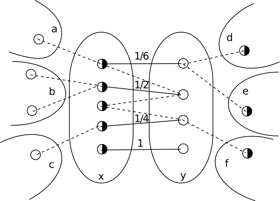
We say that the user pair ) satisfy - diversity if there is at least one event linkage set that contains co-occurring event pairs and at least of them are at different locations. However, each co-occurring event pair does not count as , since there could be many other co-occurring event pairs outside of or even that involve the same events. As such, we weight these co-occurring event pairs (detailed below). Figure 1 shows a sample event linkage set with weights for the co-occurring event pairs.
co-occurring event pairs. Let be an event linkage set in and let be a function that determines whether the co-occurring event pairs in satisfy the co-occurrence condition of - diversity. We have:
| (8) |
The weight of a co-occurring event pair is defined as:
| (9) |
Here, given a co-occurring event pair between two users, we check how many
possible users’ events could be matched to the these events. For instance,
in the figure, consider the solid line at the top with the weight .
The event on its left could be matched to events of different users,
and the event on its right could be matched to events of different users.
To compute the weight of a co-occurring pair, we multiply the inverse of these
user counts, assuming the possibility of matching from both sides are independent.
As such, in the figure, we get .
diverse event pairs.
For to be -diverse, there needs to be
at least unique locations for the co-occurring event pairs in it. However,
for a location to be counted towards these locations, the weights of the
co-occurring event pairs for that location must be at least 1. Let
denote the function that determines whether the co-occurring
event pairs in satisfy the diversity condition of - diversity. We
have:
| (10) |
Here, one subtle issue is defining a unique location. In Eq. 10 we use as the set of all unique locations. This could simply be a grid-based division of the space. In our experiments, we use the regions of the Voronoi diagram formed by cell towers as our set of unique locations.

Before we can formally state the - diversity based linkage, we have to define the alibi relation for user pairs. Let denote a function that determines whether there are more than alibi events for a given pair of users. Intuitively, having a single alibi is enough to decide that user and are not the same person, but when there is inaccurate information, disregarding candidate pairs with a single alibi event might lead to false negatives. We have:
| (11) |
With these definitions at hand, we can define the spatio-temporal linkage function that determines whether users and satisfy - diversity as follows:
| (12) |
Finally, the linkage function from the original problem formulation from Section 2.1 can be defined to contain only matching pairs of users based on , such that there is no ambiguity. Formally:
| (13) |
2.3 Example Scenario
Consider three colleagues Alice, Bob, and Carl who are working in the same office. Assume that they all use two LESs: les1 and les2. Both services generate spatio-temporal records only when they are used. The service provider would like to link the profiles of users common in both services. However, Bob uses the services only when he is at the office. On the other hand, Alice and Carl use the services frequently while at work, at home, and during vacations. Let us also assume that Alice and Carl live on the same block, but they take vacations at different locations.
When records of Alice from les1 are processed against records of Carl from les2, we will encounter co-occurrences with some amount of diversity, as they will have matching events from work and home locations. However, we will encounter alibi events during vacation time. In this case, alibi checks will help us rule out the match.
When records of Alice from les1 are processed against records of Bob from les2, the number of co-occurrences will be high, as they are working in the same office. Yet, diversity will be low, as Bob does not use the services outside of the office. This also means we will not encounter any alibi events with Alice. In this case, diversity will help us rule out the match.
In contrast to these cases, when Alice’s own usage records from les1 and les2 are processed, the resulting co-occurrences will contain high diversity since Alice uses the services at work, home, and during vacations, and will contain no alibis.
In this example scenario, high number of co-occurrences helped us distinguish between mere coincidences and potential candidate pairs. The alibi definition helped us to eliminate a false link between Alice and Carl. Finally, diversity helped us to eliminate a false link between Alice and Bob, even in the absence of alibi events.
3 ST-Link
In this section, we describe how the ST-Link algorithm implements - diversity based spatio-temporal linkage in practice. At a high-level, ST-Link algorithm performs filtering to reduce the space of possible entity matches, before it performs a more costly pairwise comparison of entities according to the formalization given in Section 2. The filtering phase is divided into two steps: temporal filtering and spatial filtering. The final phase of pairwise comparisons is called linkage.
3.1 Overview
Naïve algorithms for linkage repeatedly compare pairwise records, and thus take [17] time, where is the number of records. Such algorithms do not scale to large datasets. To address this issue, many linkage algorithms introduce some form of pruning, typically based on blocking [28, 20, 37] or indexing [19, 9]. Identifying the candidate user pairs on which the full linkage algorithm is to be run can significantly reduce the complexity of the end-to-end algorithm. Accordingly, ST-Link algorithm incorporates pruning strategies, which are integrated into the spatial filtering and temporal filtering steps.
Figure 2 shows the pipelined processing of the ST-Link algorithm. Given two sources of data for location-enhanced services (DS1 and DS2 in the figure), spatial filtering step maps users to coarse-grained geographical grid cells that we call dominating grid cells. Such cells contain most activities of the corresponding entities. Once this step is over, the remaining steps are independently performed for each grid.
The temporal filtering step slides a window over the time ordered events to build a set of candidate entity pairs. During this processing, it also prunes as many entity pairs as possible based on alibi events. As we will detail later in this section, a reverse window based scan is also performed to make sure that all relevant alibis are taken into account.
Following the spatial and temporal filtering steps, the complete linkage is performed over the set of candidate entity pairs. With a significantly reduced entity pair set, the number of compared events decreases significantly as well. Given two datasets and , the linkage step calculates as given in Eq. 13 without considering all possible entity pairs.
3.2 Spatial Filtering
By their nature, spatio-temporal data are distributed geographically. Spatial filtering step takes advantage of this, by partitioning the geographical region of the datasets into coarse-grained grid cells using a modified version of quad trees [14]. Each entity is assigned to one (an in rare cases to a few) of the grid cells, which becomes that entity’s dominating grid. The dominating grid of an entity is the cell that contains the most events from the entity. Entities that do not share their dominating grid cells are not considered for linkage. The intuition behind this filtering step is that, if entity from dataset and entity from dataset have differing dominating grids, then they cannot be the same entity.
3.2.1 Coarse Partitioning
For quad-tree generation in the ST-Link algorithm, we continue splitting the space until the grid cells size hits a given minimum. For our experiments, we make sure that the area of the grid cells is at least 100 km squares. For users, the grid cells should be big enough to cover a typical user’s mobility range around his home and work location. If the minimum grid cell size is too small, then the spatial filtering can incorrectly eliminate potential matches, as the dominating grids from different datasets may end up being different. A concrete example is a user that checks in to coffee shops and restaurants around his work location, but uses a location-based match-making application only when he is at home.
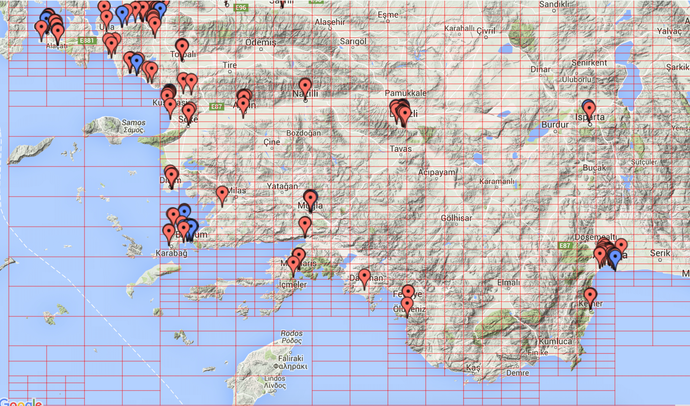
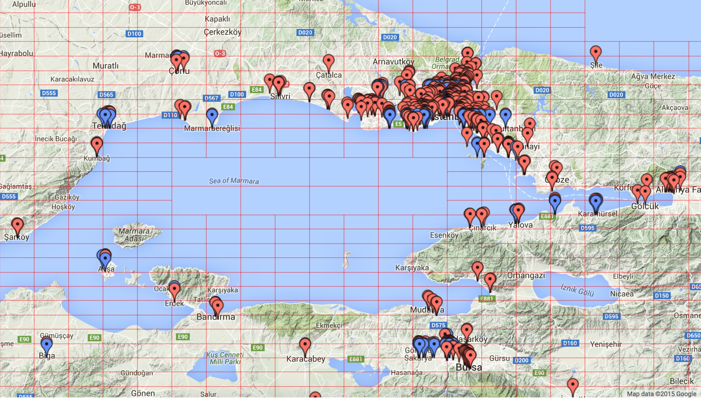
We also do not split grid cells that do not contain any events. As a result, not all grid cells are the same size. Figure 3 shows the grid cells for two selected areas in Turkey and the top 1K venues in those areas in terms of check-in counts, based on Foursquare check-in data.
3.2.2 Determining Dominating Grids
The determination of the dominating grid for an entity is simply
done by counting the entity’s events for different cells and picking the cell with the
highest count. A subtle issue here is about entities whose events end up being
close to the border areas of the grid cells. As a specific example, consider a
user who lives in one cell and works in another. In this case, it is quite
possible that a majority of the user’s check-ins happen in one cell and the
majority of the calls in another cell. This will result in missing some of
the potential matches. To avoid this situation, we make two adjustments:
If an event is close to the border, then it is counted towards the sums
for the neighboring cell(s)222An event can count towards at most 3
neighbors, in case it is at the corner of the grid. as well. We use a strip
around the border of the cell to determine the notion of ‘close to the
border’. The width of the strip is taken as the 1/8th of the minimum cell’s
edge width. This means that around of a grid overlaps with one or
more neighboring grids. This adjustment resembles the loose quad
trees [33].
An entity can potentially have multiple dominating grid cells. We have
found this to be rare for users in practice.
Figure 3(b) shows the resulting grids over selected areas in Turkey,
and the most popular venues from our dataset. Red pins are
showing the venues and the blue ones are showing the ones that count towards
neighboring grids.
3.2.3 Forming Partitioned Datasets
Once the dominating grid cells of users are determined, we create grid cell specific datasets. For a given grid cell , we take only the events of the entities who has as a dominating grid cell. These events may or may not be in the grid cell . Determination of the dominating grid cells of entities requires a single scan over the time sorted events from entities. The forming of the partitioned datasets requires a second scan.
3.3 Temporal Filtering
Temporal filtering aims at creating a small set of candidate user pairs on which the full linkage algorithm can be executed. To create this set, temporal filtering looks for user pairs that have co-occurring events, as expressed by Eq. 3. Importantly, temporal filtering also detects alibi events, based on Eq. 5, and prevents user pairs that have such alibi events from taking part in the candidate pair set.
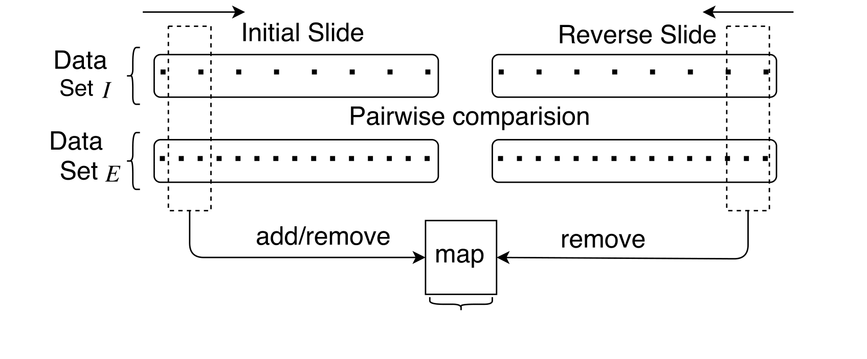
Temporal filtering is based on two main ideas. First, a temporal window is slided over the events from two different datasets to detect user pairs with co-occurring events. Since co-occurring events must appear within a given time duration, the window approach captures all co-occurring events. Second, as the window slides, alibi events are tracked to prune the candidate user pair set. However, since the number of alibis is potentially very large, alibis are only tracked for the user pairs that are currently in the candidate set. This means that some relevant alibis can be missed if the user pair was added into the candidate set after an alibi event occurred. To process such alibis properly, a reverse window scan is performed, during which no new candidate pairs are added, but only alibis are processed. Algorithm 1 gives the pseudo-code of temporal filtering.
3.3.1 Data Structures
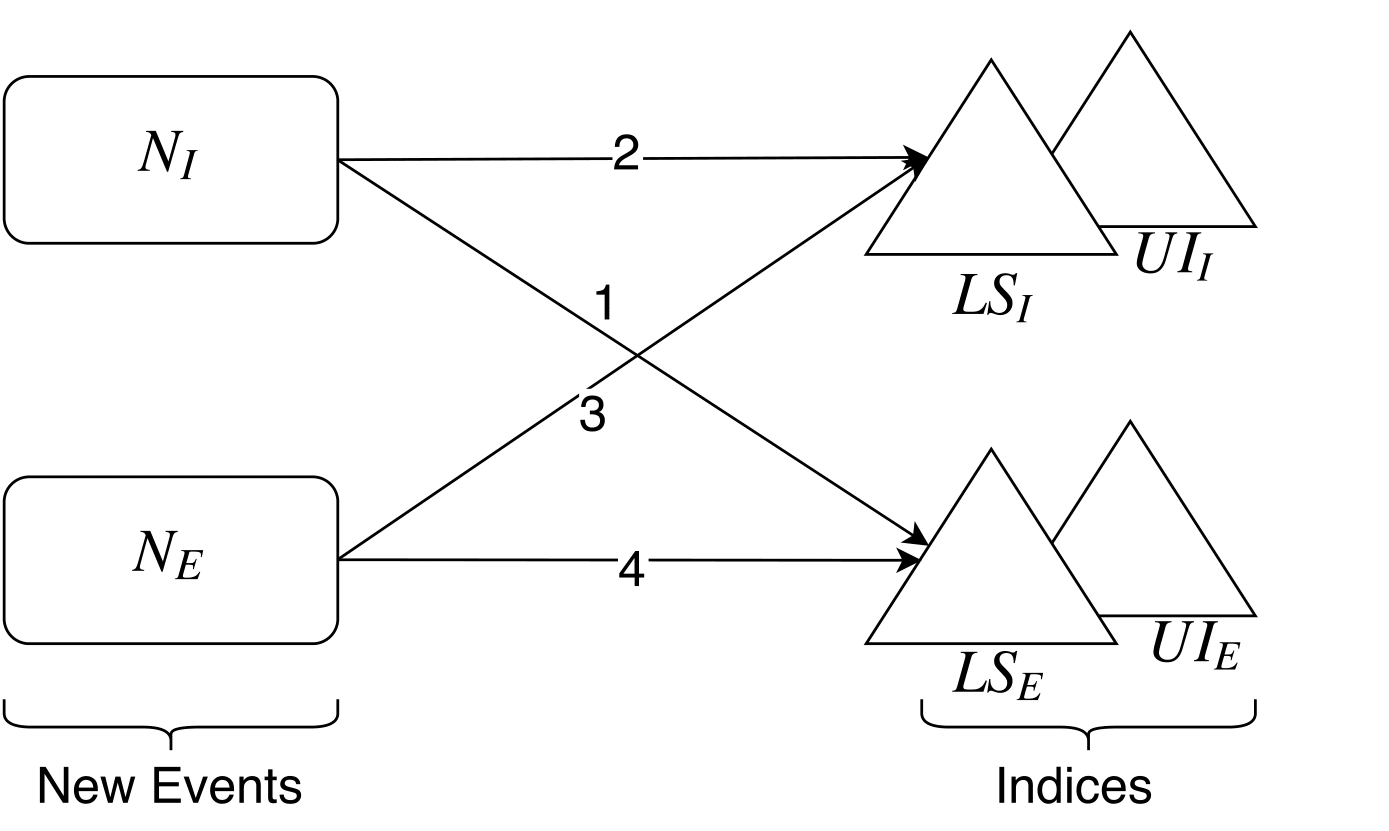
A window of size (see Eq. 2) is slided jointly over both time sorted datasets. Figure 4(a) depicts this visually. Each time the window slides, some events from both datasets may enter and exit the window. We utilize two types of data structures to index the events that are currently in the window. The first type of index we keep is called the user index, denoted by , where . In other words, we keep separate user indexes for the two datasets. is a hash map indexed by the user. keeps all the events (from dataset ) of user in the window. As we will see, this index is useful for quickly checking alibis.
The second type of index we keep is called the spatial index, denoted by , where . Again, we keep separate indexes for the two datasets. could be any spatial data structure like R-trees. gives all events whose region intersect with region . As we will see, this index is useful for quickly locating co-occurring events.
In addition to these indexes, we maintain a global candidate set and a global alibi set . For a user (from either dataset, assuming user ids are unique), keeps the current set of candidate pair users for ; and keeps the current known alibis users for . It is important to note that is not designed to be exhaustive. For a user , only keeps alibi users that have co-occurring events with in the dataset.
3.3.2 Processing Window Events
The algorithm operates by reacting to events being inserted and removed from the window as the window slides over the dataset. As a result, an outermost while loop that advances the window until the entire dataset is processed. At each iteration, we get a list of events inserted ( and ) and removed ( and ) from the window. We first process the removed events, which consists of removing them from the spatial and user indexes. We then process the inserted events. We first process against and , then insert the events in into and , then process against and , and finally insert the events in into and . This ensures that all the events are compared, and no repeated comparisons are made. Figure 4(b) depicts the order of events visually.
To compare a new event from dataset against the events from dataset that are already indexed in the window (where ), we use the indexes and . First, we find events that co-occur with by considering events in . These are events whose regions intersect with that of . If the user of such an event is not already a known alibi of the user of (not in ) and if the co-occurrence condition is satisfied, then the user and user are added as candidate pairs of each other. Second, and after all the co-occurrences are processed, we consider all candidate users of the event ’s user, that is , for alibi processing. For each user in this set, we check if any of its events result in an alibi. To do this, we iterate over user ’s events with the help of the index . In particular, for each event in , we check if and are alibis, using the condition . If they are alibis, then we remove and ’s user () from each other’s candidate sets, and add them to their alibi sets.
This completes the description of the forward scan of the window. An important point to note is that, during the forward window scan, we only check alibis for user pairs that are in the set of candidate pairs. It is possible that there exists an alibi event pair for users and , that appears before the first co-occurring event pair for these users. In such a case, during the processing of the alibi events we won’t have this pair of users in our candidate set and thus their alibi will be missed. To fix this problem, we perform a reverse scan. During the reverse scan, we only process alibis, as no new candidate pairs can appear. Furthermore, we need to process alibi events for a user pair only if the events happened before the time this pair was added into the candidate set. For brevity, we do not show this detail in Algorithm 1. At the end of the reverse scan, the set contains our final candidate user pairs, which are sent to the linkage step. Temporal filtering is highly effective in reducing the number of pairs for which complete linkage procedure is executed. The experimental results show the effectiveness of this filtering.
When there is inaccurate information in the datasets, disregarding candidate pairs due to only a single alibi event might lead to false negatives. However, the algorithm is easily modifiable to use a threshold for alibi values. In this modified version, we update the structure of the alibi set to keep the number of alibi events of a pair as well. Now keeps the current known alibi users of user with alibi event counts for each. Just like in the original algorithm, when two events and are compared we first check if the number of alibi events of users and exceeds the threshold. To avoid double counting, we reset the counters before the reverse scan. Since all alibi events of current candidate pairs will be counted in reverse scan, candidates whose count of alibi events exceed threshold will not be included in the resulting candidate set .
So far we have operated on time sorted event data and our algorithms used only sequential I/O. However, during the linkage step, when we finally decide whether a candidate user pair can be linked, we will need the time sorted events of the users at hand. For that purpose, during the forward scan, we also create a disk-based index sorted by the user id and event time. This index enables us to quickly iterate over the events of a given user in timestamp order, which is an operation used by the linkage step. For this purpose, we use LevelDB [18] as an index, which is a log-structured merge-tree supporting fast insertions.
While writing the event to the disk-based index, we also include information about the number of unique users the event has matched throughout its stay in the forward scan window. This information is used as part of the weight calculation (recall Eq. 9) in the linkage step.
3.3.3 Handling Time Period in Events
The temporal filtering step scans time-ordered events by sliding a window of size over them. This operation assumes that the time information is a point in time. Yet, there could be scenarios where the time information is a period (e.g., a start time and a duration). However, frequently, these records contain only start location of the event. For example, although Call Detail Records (CDR) have the start time of the call and the duration, they usually contain only the originating cell tower information. Considering mobility of the users, assuming a fixed location during this period would lead to location ambiguity.
If we have events with time periods and accurate location information is present during this period, we can adapt our approach to handle this. In particular, we need to avoid false negative candidate pairs when the event contains a time period. Since events are processed via windowing, making sure that the event with the time period information stays in the window as long as its time period is valid would guarantee that all co-occurrences will be processed. This requires creating multiple events out of the original event, with time information converted into a point in time and the correct location information attached to it. The number of such events is bounded by the time duration divided by the window size, .
3.4 Linkage
The last step of the ST-Link algorithm is the linkage of the entities that are determined as possible pairs as a result of spatial and temporal filtering. This linkage is a realization of the - diversity based linkage model introduced in Section 2. Given two entities from two datasets, the linkage step uses the events of them to determine whether they can be linked according to Eq. 12. Thanks to efficient filtering steps applied on the data beforehand, the number of entity pairs for which this linkage computation is to be performed is significantly reduced.
For each entity pair, their events are retrieved from the disk-based index created as part of the forward scan during the temporal filtering. These events are compared for detecting co-occurring events. Co-occurring events are used to compute the value, via simple accumulation of the co-occurrence weights. They are also used to accumulate weights for the places where co-occurring events occur. This helps us compute the value, that is diversity. After all events of a pair of entities are compared, we check if they satisfy the - diversity requirement. Note that, it is not possible to see an alibi pair event at this step, as they are eliminated by the temporal filtering step.
There are a number of challenges in applying the --diversity based linkage. The first is to minimize the number of queries made to the disk-based index to decrease the I/O cost. Events from the same entity are stored in a timestamped order within the index, which makes this access more efficient. Also, if one of the datasets is more sparse than the other, then the linkage can be performed by iterating over the entities of the dense datasets first, making sure their events are loaded only once. This is akin to the classical join ordering heuristic in databases.
Another challenge is the definition of the place ids to keep track of diversity. A place id might be a venue id for a Foursquare dataset, store id for credit card payment records, cell tower id for Call Detail Records, or a geographic location represented as latitude and longitude. An important difference is the area of coverage for these places. Consider two datasets of Foursquare check-ins and Call Detail Records, and places based on venues. If a user visits several nearby coffee shops and makes check-ins and calls, these will be considered as diverse even though they are not geographically diverse. The use of cell tower coverage areas is a more practical choice for determining places.
The last challenge is about matching events. Recall from Figure 1 that events of two entities can be matched in multiple different ways, resulting in different weights for the co-occurrences. Ideally, we want to maximize the overall total weight of the matching, however this would be quite costly to compute, as the problem is a variation of the bipartite graph assignment problem. As a result, we use a greedy heuristic. We process events in a timestamped order and match them to the co-occurring event from the other entity that provides the highest weight. Once a match is made, event pairs are removed from the dataset so that they are not re-used.
Different - value pairs may perform significantly different in terms of precision and recall, depending on the frequencies of the events in the datasets. An ad-hoc approach is to decide the and values based on observation of results from multiple experimental runs. A more robust technique we used is to detect the best trade-off point (a.k.a elbow point) on a curve. Given the co-occurrence and diversity distributions, we independently detect the elbow point of each, and set the and values accordingly. Although there is no unambiguous solution for detecting an elbow point, the maximum absolute second derivative is an approximation. Let be an array of co-occurrence (or diversity) values with size . Second derivative, , of point at index can be approximated with a central difference as follows:
| (14) |
The value at index , such that has the maximum absolute value, is selected as the elbow point and (or ) value is set accordingly.
4 Experimental Evaluation
In this section, we present an evaluation of the proposed - diversity based linkage method and the ST-Link algorithm. We implemented the ST-Link algorithm using Java 1.7. All experiments were executed on a Linux server with Intel Xeon E5520 GHz CPUs and GB of RAM.
We present two sets of experiments. In the first set of experiments, we measure the performance and the scalability of the ST-Link algorithm. By increasing the size of the input data, we test the change in the running time, number of event comparisons, and the number of candidate user pairs, for different window sizes. In the second set of experiments, we analyze the quality of the - diversity based linkage. To measure quality, we use two metrics. The first is the precision, which measures the fraction of correctly linked pairs in the list of user pairs produced by ST-Link. The second is the number of true positives, which is the number of user pairs correctly linked by the ST-Link algorithm.
4.1 Datasets Used
For the performance, scalability, and accuracy evaluations we used three datasets. The first is a Foursquare dataset of check-ins. The second is anonymized call detail records in a telecommunication provider. For privacy concerns, we did not perform any linkage across these two datasets. As a result, we were not able to compute accuracy results when using these two datasets. However, they are used for the evaluation of running time performance. To evaluate accuracy, linkage is performed between a third dataset belonging to a hypothetical LES and the call dataset. This dataset was synthetically derived to protect privacy, from the call dataset by () picking a predefined fraction of the callers at random as active users of the second LES, () generating usage records for the selected users by assuming that they generate such a record with probability , within a minute time window of a call, inside a location within the same cell tower of the call. We change the parameters and to experiment with different scenarios. Lower values for result in a sparser usage record dataset for the second LES. We call the parameter , the check-in probability. As not all users have the same check-in probability in practice, we pick the value of the check-in probability for a given user from a Gaussian distribution with mean . We call the parameter , the usage ratio.
| Datasets | Foursquare | Call |
|---|---|---|
| # of activities | 1,903,674 | 1,890,107,057 |
| # of venues/cell towers | 300,685 | 109,780 |
| # of users | 284,856 | 3,357,069 |
The Foursquare dataset consists of check-ins that were shared publicly on Twitter, collected via the Twitter streaming API333www.dev.twitter.com and the Foursquare API444www.developer.foursquare.com. This dataset spans days and only contains check-ins from Country X. Each row contains the acting user’s Foursquare id, venue id, geographical location (lat/lon) of the venue, and the time of the check-in. The call dataset spans the same days in Country X. Each row contains an anonymized id, time of the call, and geographical location (lat/lon) of the handling cell tower. The anonymized id is the same across all usage of the same user. Table I shows the statistics about both the Foursquare and the call datasets. For the runtime performance and filtering effectiveness experiments, we used the two real datasets. However, since it is not possible to verify the accuracy of the results using these two datasets, we used the synthetic dataset which is derived from the anonymous call data for the evaluation of ST-Link’s accuracy.
4.2 Running Time Performance
| Precision | Recall | |
|---|---|---|
| 2-2 | 0.19 | 0.31 |
| 3-2 | 0.36 | 0.32 |
| 3-3 | 0.89 | 0.61 |
| 4-3 | 0.93 | 0.47 |
| 4-4 | 0.99 | 0.58 |
| 5-4 | 0.99 | 0.47 |
| 5-5 | 0.99 | 0.50 |
We observe the running time, the number of candidate pairs, and the number of event comparisons as a function of the dataset size. The dataset size is increased by increasing the number of days of data included in the linkage analysis. Furthermore, for these experiments we also change the window size. Recall that the window size is used during the temporal filtering step to locate co-occurring events.
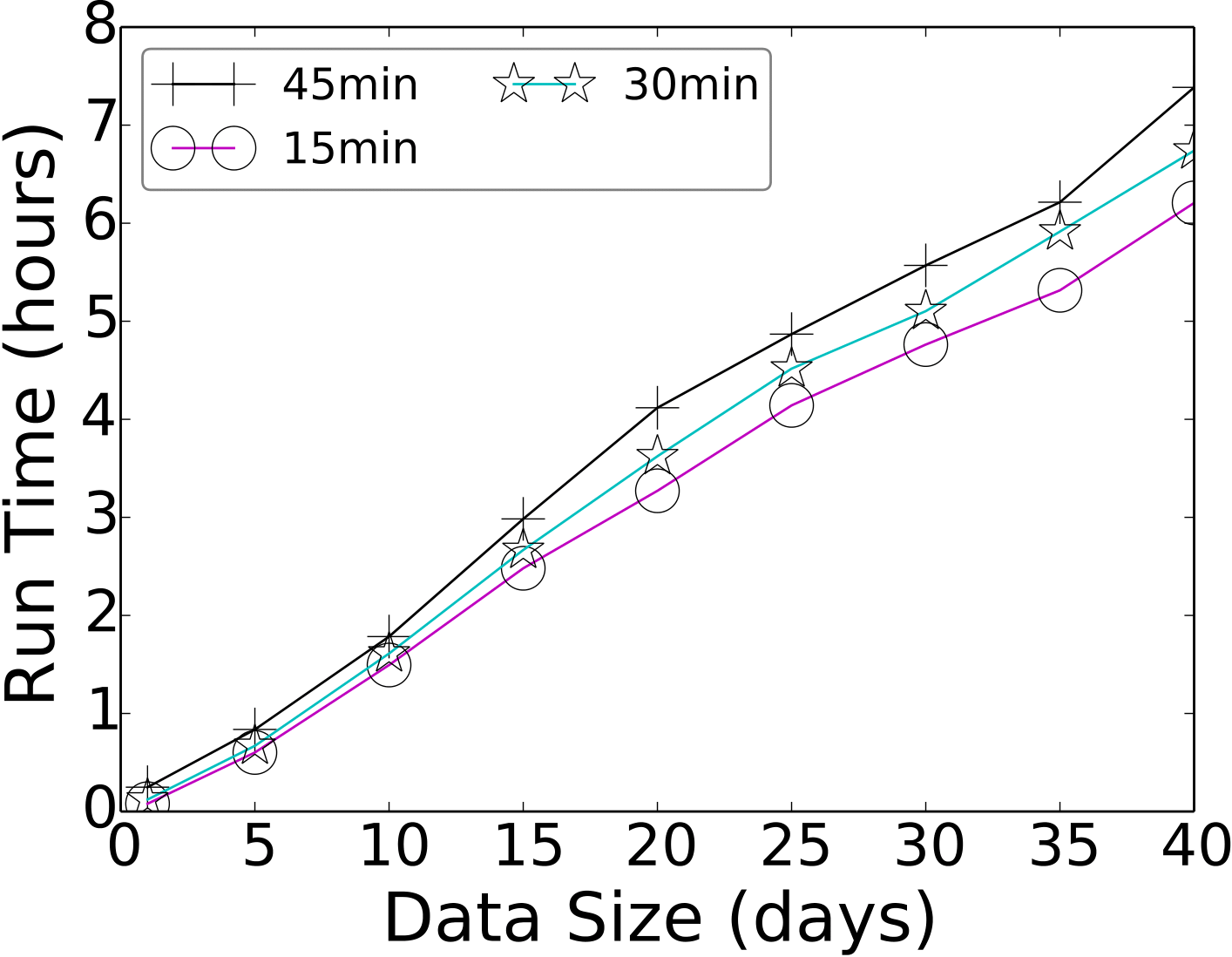
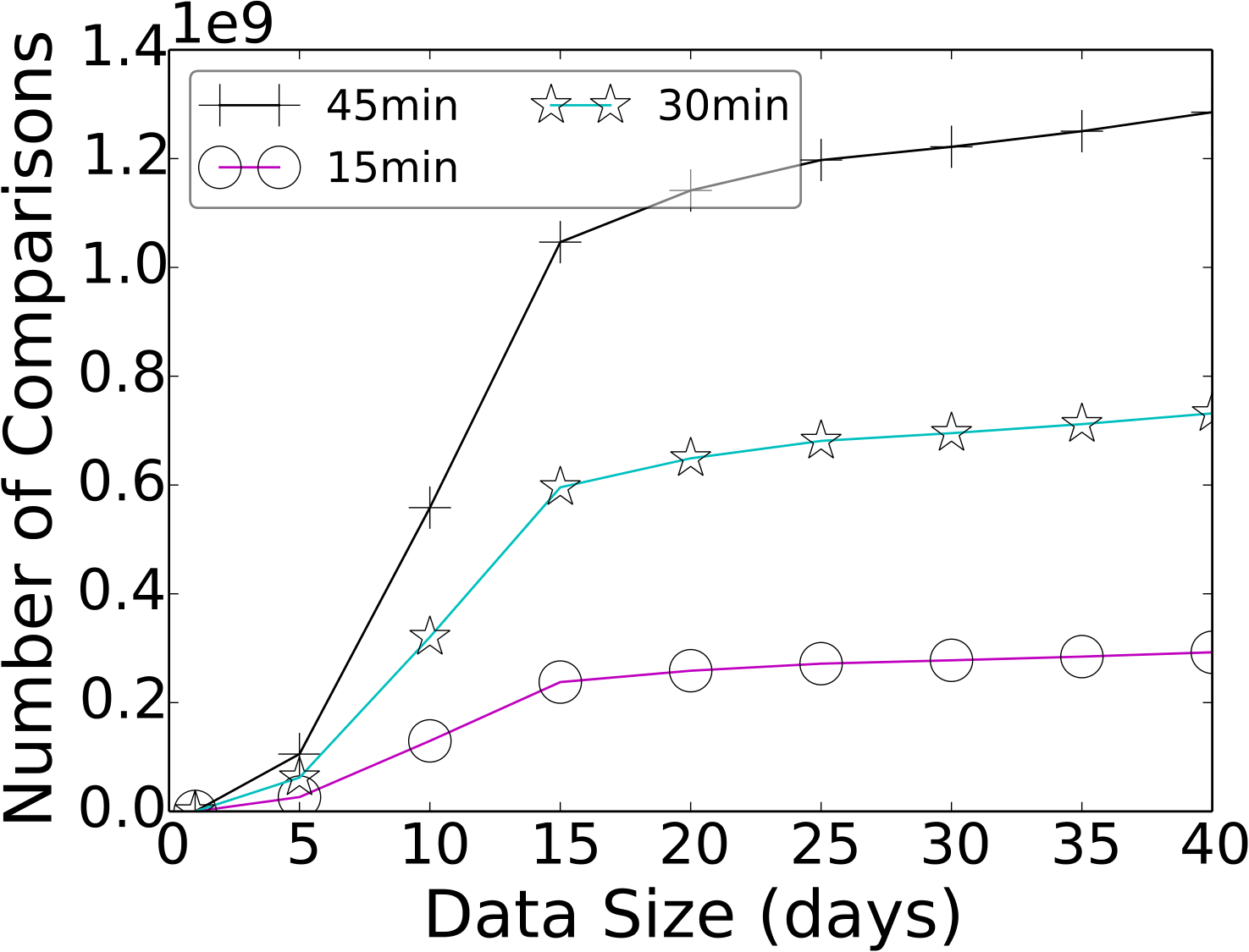
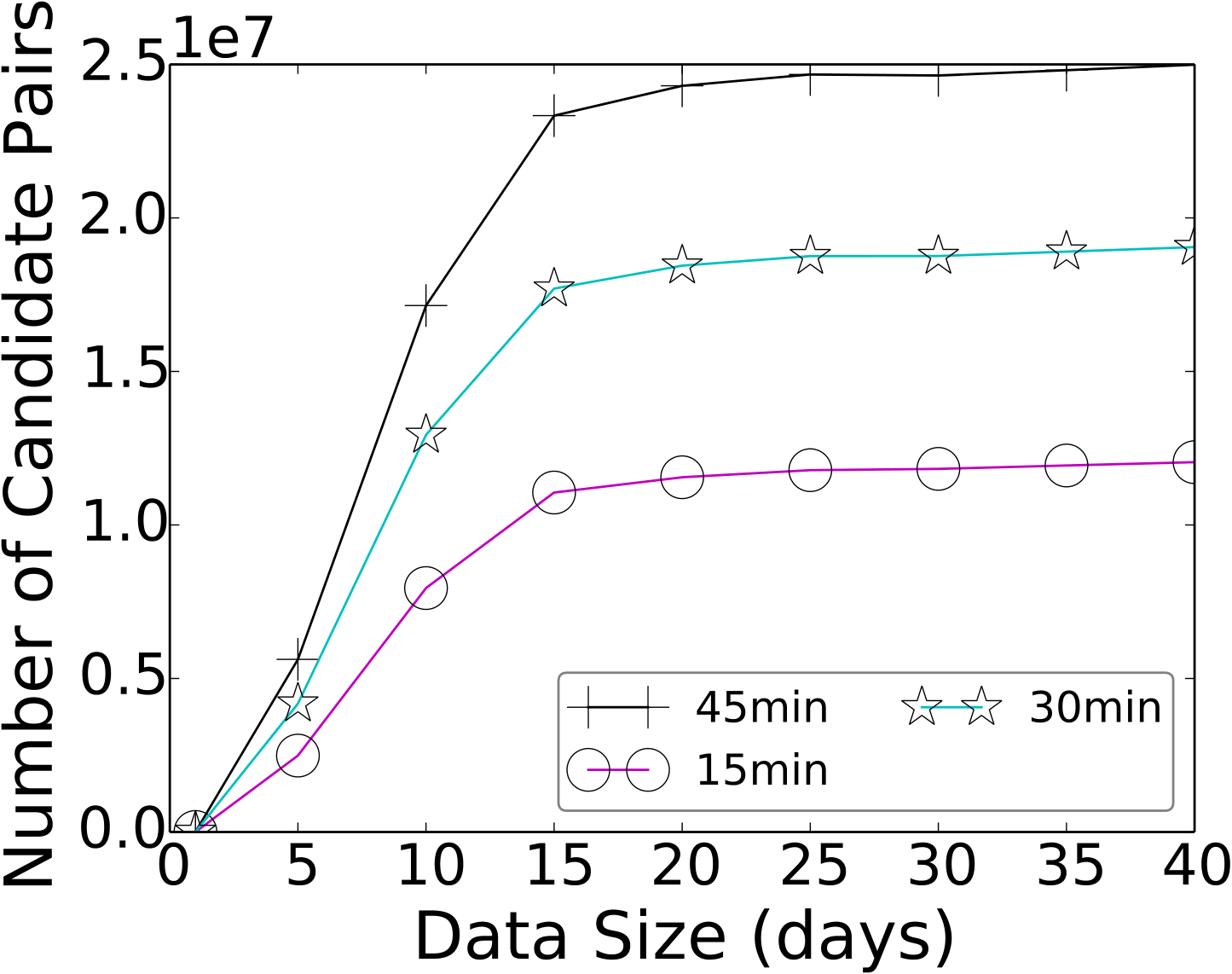
Figure 5 presents our running time related results. In all the figures, the -axis represents the dataset size in days and the -axis represents a performance metric. Different series represent varying window sizes.
One of the main challenges is the scalability of the linkage solution. Processing many days of data should complete in reasonable amount of time for the resulting analysis to be valuable. Figure 5(a) plots the running time as a function of the dataset size. We make two observations from the figure. First, the running time of ST-Link is linear in the dataset size. For 5 days of data, the running time is around hour and for days of data it is around hours, all for minute windows. Second, the running time increases with increasing window size, yet the running time is linear in the dataset size for all window sizes.
Figure 5(b) plots the number of event-to-event comparisons as a function of the dataset size. In our experimental evaluation, every time we compare two location based events for either co-location or alibi check, the number of event comparisons is increased by one. We observe that up to 15 days of data, the number of comparisons grows at an increasing rate. Yet, after 15 days the rate starts to go down and eventually the growth of the number of operations happens at a relatively low fixed rate. This can be explained by the alibi checks performed by ST-Link. Recall that when a user pair is marked as an alibi, their records are not compared with each other anymore. Also, if two users are marked as a candidate pair, their future records are only compared to see if they are an alibi or not. Considering this, we can say that within 15 days most of the candidate pairs and alibi pairs are identified. As an important difference from the running time experiment, the gaps between the series corresponding to the three window sizes are considerably larger. This is because larger windows require more event to event comparisons. Since event comparisons are not necessarily the only cost of the algorithm (there is I/O, window processing, window index maintenance, etc.), the running time experiment has narrower gaps between the running times for different window sizes. The impact of these extra costs can be seen in Figure 5(a) as well; although the number of comparisons stabilize after 15 days, the linear increase in the runtime continues.
Figure 5(c) plots the number of candidate user pairs as a function of the dataset size. Just like for the number of comparisons experiment, up to 15 days, the number of candidate pairs grows with an increasing rate and after 15 days the rate starts to decrease and eventually stabilizes at a low value. For the case of candidate pairs, the eventual rate of increase is very low, suggesting that observing additional data brings diminishing returns in terms of being able to find new candidate pairs. However, this does not imply that we are unable to perform additional linkages, because the number of linked pairs within the candidate set can still grow (we will observe such growth in the quality experiments).
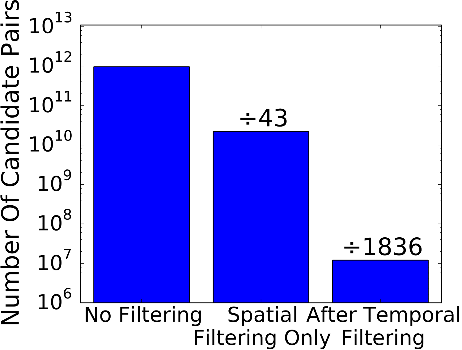
Figure 8 shows the number of candidate user pairs after each filtering step. It illustrates the effectiveness of the spatial and temporal filtering steps of ST-Link. If no filtering was applied on the data, every user pair from the two datasets would have constituted a candidate user pair. By applying only spatial filtering, the number of candidate user pairs decreases by times compared to the no filtering case. It is possible to say that spatial filtering is an effective step. Intuitively, if data was spread over a wider geographical area, this step would be have been even more effective (our datasets are limited to the geographic area of Country X). After applying temporal filtering, the candidate user set decreases by an additional times after spatial filtering. Cumulatively, the number of candidate user pairs without any filtering is times of the number of pruned candidate user pairs, which gets close to orders of magnitude reduction in the number of pairs.
4.3 Quality of Linkage
We observe the precision and the number of true positives as a function of the usage ratio, check-in probability, and window size. We also observe the precision and recall values for a variation of the ST-Link algorithm that does not use weights, thus trades off precision for better recall.
4.3.1 Impact of Check-in Probability
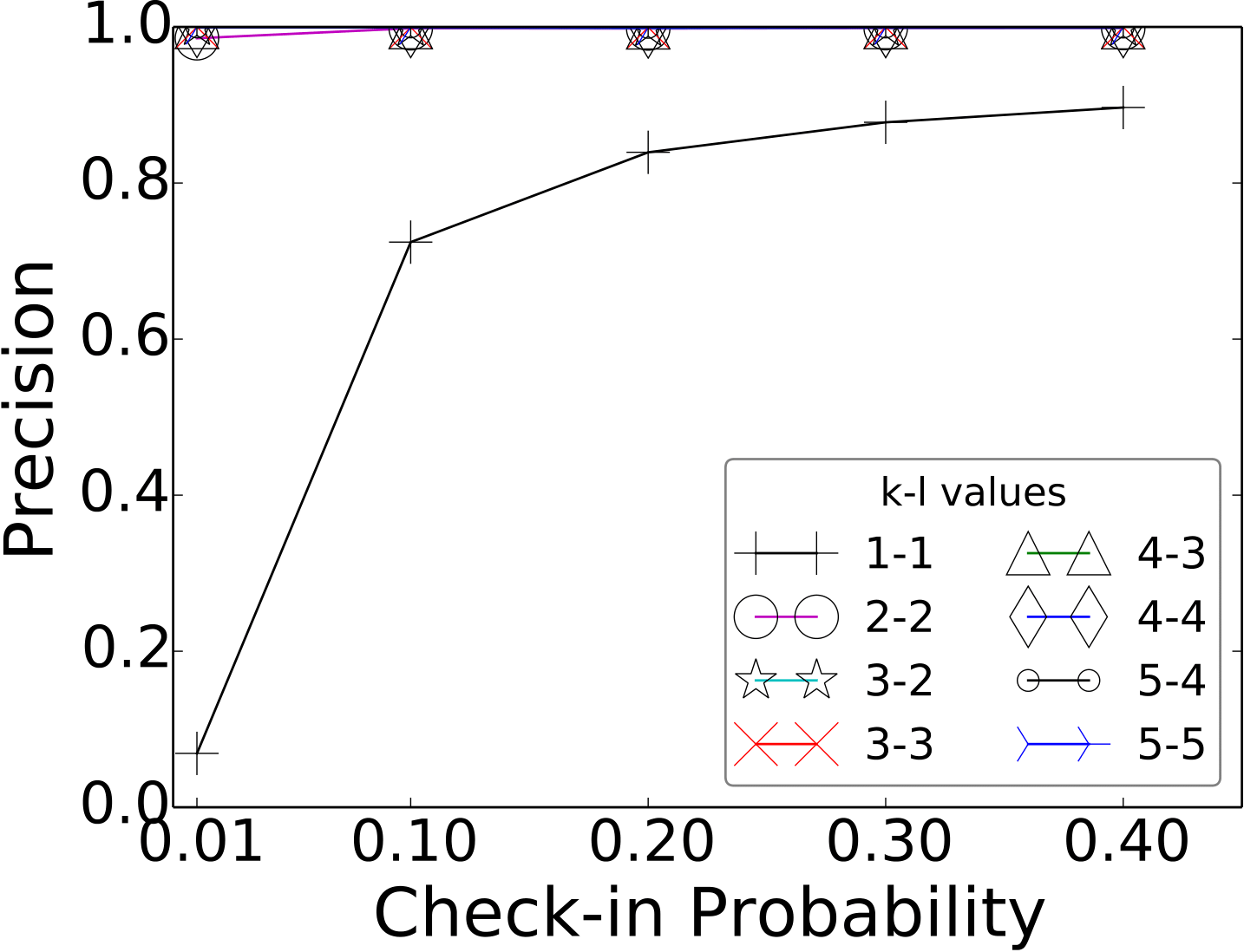
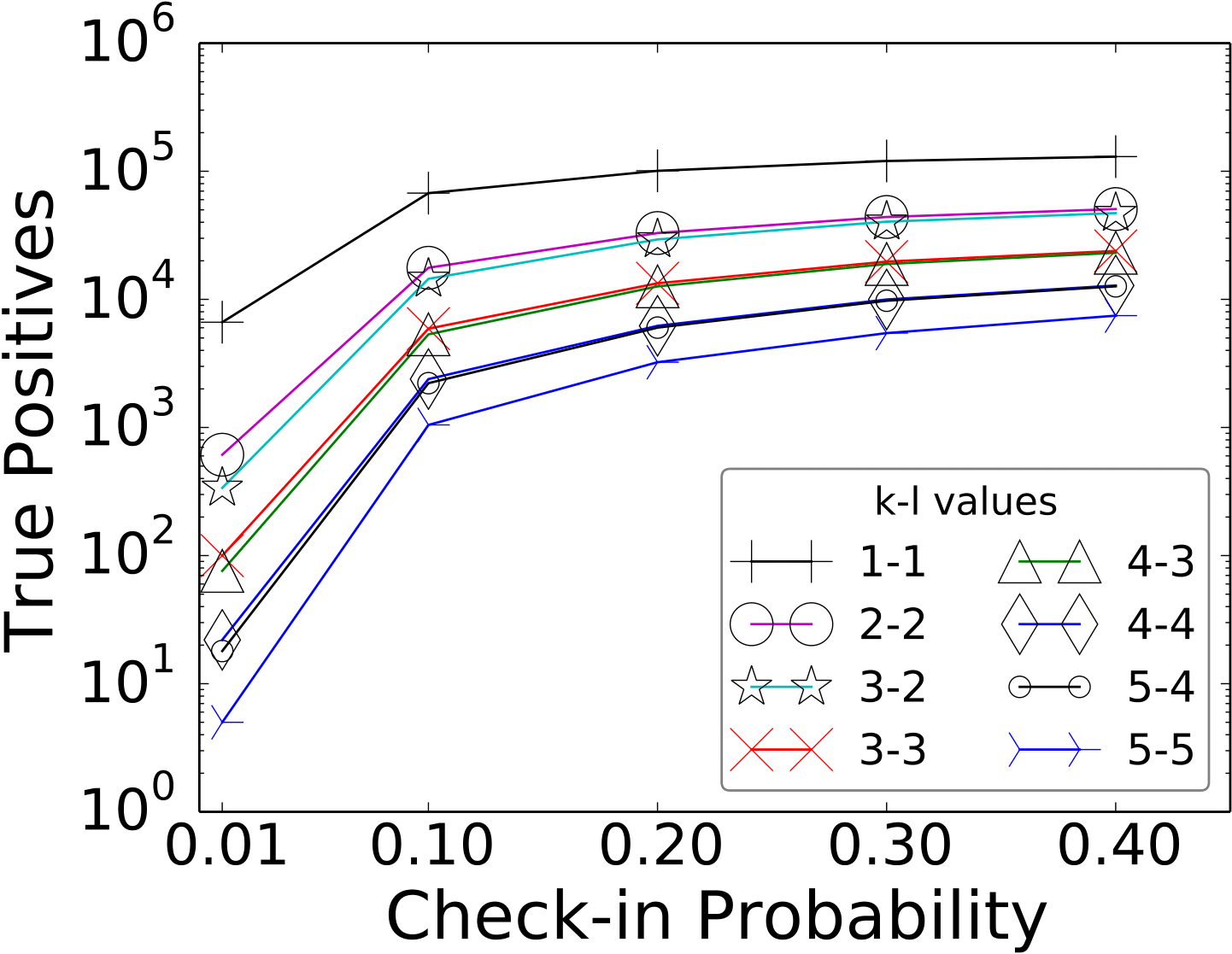
Figures 8 and 8 plot the precision and number of true positives, respectively, for the results produced by the ST-Link algorithm as a function of the mean check-in probability. Different series in the figure represent different - settings. We set , as the co-occurrence counts has to be greater than the diversity counts. For these experiments the usage ratio is set to , which means only half of the call users are performing check-ins.
Figure 8 shows that precision is very close to for all - settings but for -. We see that using - diversity results in very poor precision for low values of the check-in probability. As the check-in probability increases, then the precision of - diversity increases as well, but never reaches . The increase is understandable, as more events on the check-in side will help rule out incorrect candidate pairs via alibis. Surprisingly, the precision for higher - values are all close to . This is due the impact of alibi detection, and strong weight constraint. As we will see shortly, not using weights trades off precision for better recall. Even if two users have events that are only - diverse, they can be correctly linked if they have no alibis.
Figure 8 shows that the number of true positives in the linkage increases with the increasing check-in probability. This is expected, as more events help in increasing the co-occurrence and diversity counts. We also observe that higher - values result in reduced number of linkages. Given that - diversity has very good precision, and has the second highest true positive count (after - diversity, which has unacceptable precision), it can be considered a good setting for getting the best out of the linkage. We see that for a check-in probability as low as , it can match many hundreds of users, and for probability , it can match up to thousand users. As we will see shortly, these numbers can be further increased by trading off some accuracy.
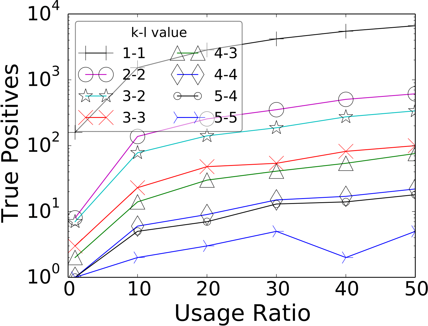
4.3.2 Impact of Usage Ratio
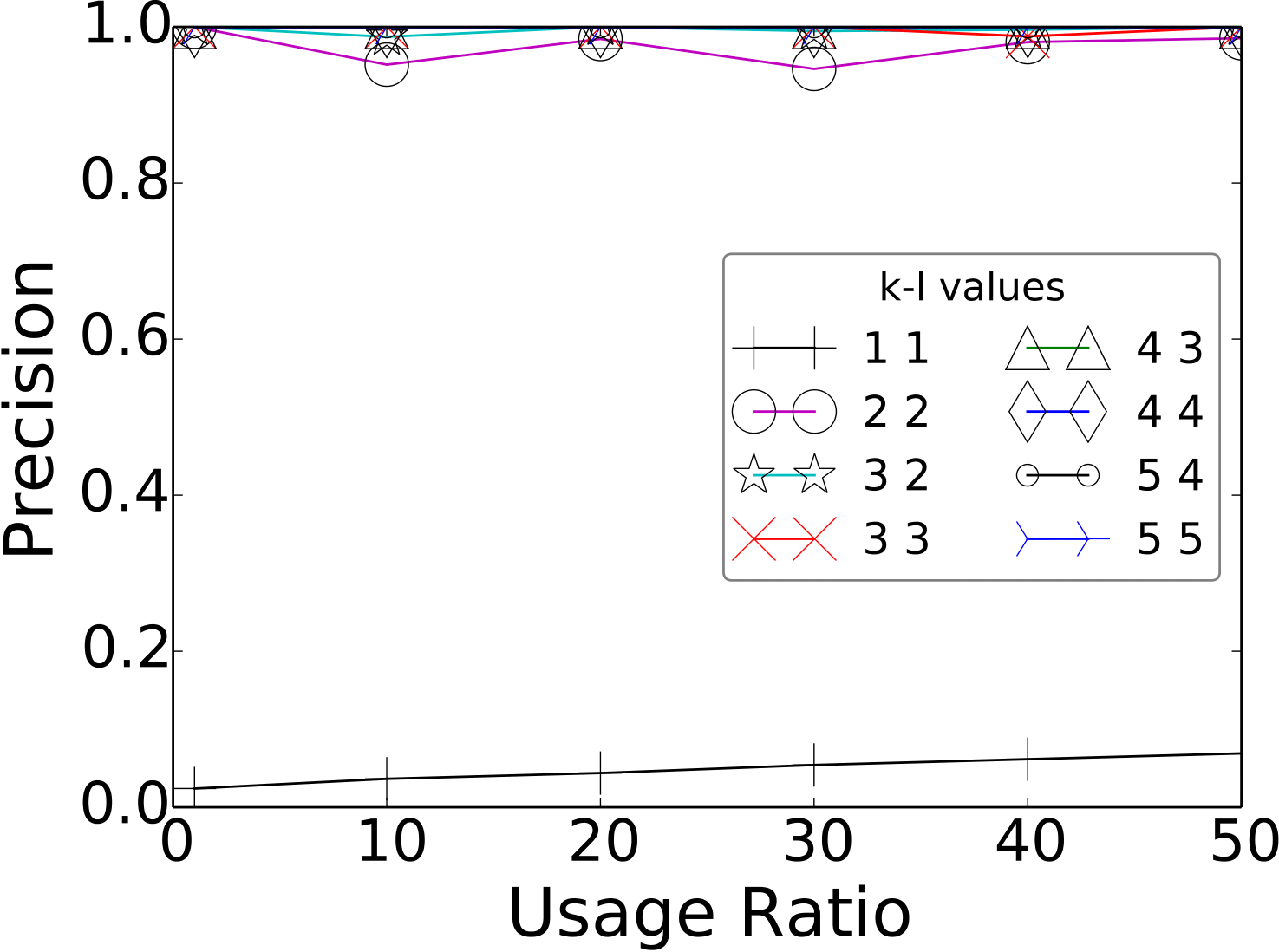
Figures 11 and 11 plot the precision and the number of true positives, respectively, for the results produced by the ST-Link algorithm as a function of the usage ratio. Different series in the figure represent different - settings, as before. For these experiments check-in probability is taken as .
Figure 11 shows that the precision of all - settings is close to throughout the entire range of the usage ratio, except for -. The - setting has precision values that are slightly lower than , but not lower than . Figure 8 shows the true positive counts for the same settings. As we can see clearly from the figure, increased usage ratio results in increased number of successful linkages. Again, this could be attributed to increasing weights for co-occurrence and diversity, as well as increased effectiveness of alibi detection.
Interestingly, even when only percent of the call users are synthetically set to making check-ins, and when the check-in probability around a call is set as low as in , one can still match some users (around ). This could also be looked at from a privacy standpoint. In other words, being able to perform spatio-temporal linkage across two datasets successfully even for only users may be considered a privacy breach. We plan to investigate the privacy protection mechanisms against this kind of linkage in our future work.
4.3.3 Unweighted Linkage
The results so far have demonstrated high precision, but the number of users one could match is relatively low compared to the number of total users. In order to show the trade-off between precision and accuracy, we have also performed experiments where the linkage model is slightly modified to use weights that are equal to . That is, we count each event co-occurrence between two users as , without considering other possible co-occurrences these events may have with events of other users. In other words, the weight function from Eq. 9 is taken as . As it was discussed before, there are two different approaches for deciding the values of the - parameters. The first one is deciding after multiple experimental runs, and the second one is by detecting the elbow point of distributions of co-occurrence and diversity values.
In this experiment we applied both to show the effectiveness of the elbow point detection technique as well. According to maximum absolute second derivative test results, the values of - parameters based on elbow detection are -.
Table 11 shows the precision and recall results for the unweighted linkage. The recall values here represent the fraction of users from the check-in dataset that were successfully linked. It is important to note that we only considered users that have enough number of events. A user is said to have enough number of events only when she has at least diverse events, for each - setting. The table shows an interesting result: With unweighted linkage we see a clear tradeoff, where with increasing - values the precision improves, but the recall drops. With the - setting, we get a precision of and can link of the users that have enough number of events. Considering all users from the check-in dataset this value is . Recall that - setting was identified using the elbow points. Increasing the diversity setting to -, one gets almost perfect accuracy (), but the recall drops to of the users. When absolute accuracy is not required, such as for machine learning to extract overall patterns, the unweighted linkage model could be more effective in practice.
4.3.4 Impact of Alibi
| Runtime (m) | Precision | Recall | Cand. Count | |
|---|---|---|---|---|
| 1 | 30 | 0.78 | 0.68 | 1,998,491 |
| 2 | 34 | 0.75 | 0.74 | 2,651,746 |
| 4 | 39 | 0.71 | 0.82 | 3,511,090 |
| 8 | 45 | 0.68 | 0.88 | 4,446,937 |
| 16 | 58 | 0.65 | 0.91 | 5,311,043 |
| 122 | 0.62 | 0.99 | 6,765,345 |
Alibis are used to improve both the running time performance and the accuracy.
For these experiments the check-in probability is taken as and the
usage ratio is taken as . Only one grid is considered, which contains
15,268 users and 1,956,734 events in total. As it was discussed before, a threshold value
on the number of alibi events can be used before disregarding a candidate pair. In this
experiment we evaluate the impact of alibi in terms of performance and accuracy as a function of the alibi threshold.
Performance.
Table 15 shows the running time, precision, recall, and
the number of candidate pairs for the alibi threshold experiment. When the
threshold is set to , effectively disabling alibi detection, we
observed that the algorithm took 122 minutes to complete. At the end of the
temporal filtering step, there were 6,765,345 possible pairs. On the other
hand, when alibi is used and the threshold is set to , the running time
decreased down to 30 minutes and the number of possible pairs were 1,998,491.
Almost of the possible pairs were pruned with the help of alibi
detection and further processing is avoided. When larger threshold values are
used, we observe slight increase in the running time. For the threshold values
of and , the processing time is and minutes, respectively.
Accuracy. Precision of the - diversity based linkage can
be increased by setting sufficiently large and values. Larger and
values decrease the probability of different users satisfying the linkage
requirements. However when at least one of the datasets is sparse, setting
larger and values will result in low recall, as many true positive
pairs will be missed. In such datasets, alibi definition prevents many false
positive pairs that satisfy the co-occurrence and diversity requirements. Our
experiments showed that when alibi is not used (threshold value ), recall can be reached, yet with precision. In contrast, setting
alibi threshold to , increases the precision to , with recall
decreased to . The reason behind this decrease has to do with the lack
of precise location information in our datasets. For example, when two
temporally close events of a user are from two neighboring cell towers, their
locations end up being the centers of the cell towers, as the location
information is not sufficiently fine grained. This results in
incorrectly identifying a pair of events as alibis, as the distance between
the event locations is relatively high when considering their close
timestamps. This is when the alibi threshold becomes crucial. We observe that
the recall increases to when alibi threshold set to . Increasing
threshold further increases the recall values with a cost of sacrificed
precision. For alibi threshold recall is and precision is .
4.3.5 Window Size
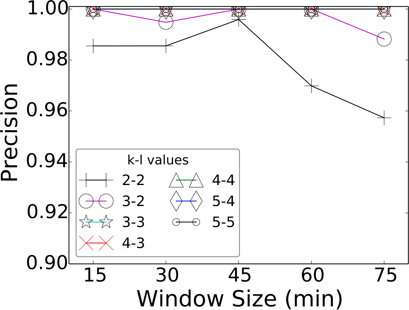
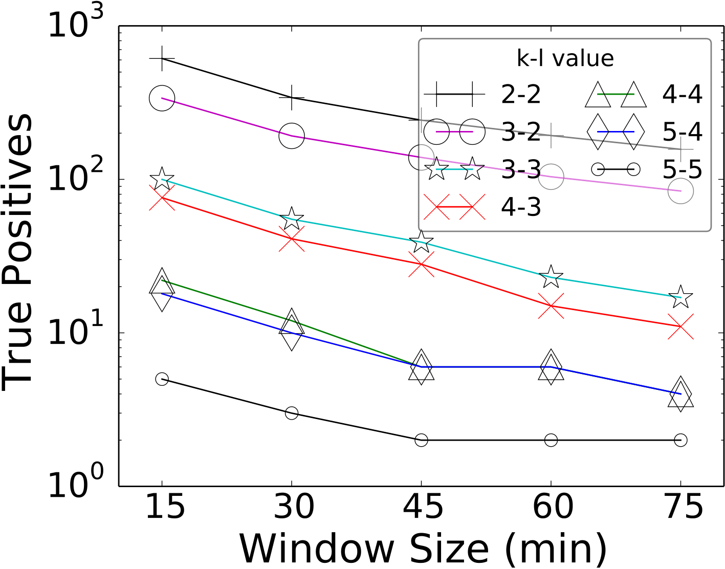
Figures 14 and 14 plot the precision and the number of true positives, respectively, as a function of the window size. Different series in the figure represent different - settings, as before. For these experiments the check-in probability is taken as and the usage ratio is taken as . Window sizes start from minutes and increases up to minutes in increments of minutes.
Figure 14 shows that the precision stays at is not effected by the window size except for lines corresponding to lower - values. In particular - and - are impacted negatively from larger window sizes. - is not shown in this experiment, as it already has a very low precision. Note that the window size does not impact only the size the temporal window we slide over the events, but also the definition of co-occurrence (recall the parameter from Eq. 2). Increasing the window size makes it possible to match potentially unrelated events from different real-world users and the results reflect that. However, due to the alibi processing, the negative impact of increasing window size on the precision is milder that it would otherwise be.
Figure 14 shows that the number of true positives drops with increasing window sizes. Again this can be attributed to the increasing number of unrelated event matches due to the larger window. Recall that if the same user is matched to more than one user from the other dataset, we remove such users from the linkage results. The increased window size results in ambiguity in the results. Assuming users and are linked for a given window size, increasing the window size does not change the fact that and are matched, but it may result in additional matches, such as between user and some other user , and thus eliminating the correct linkage between and from the results.
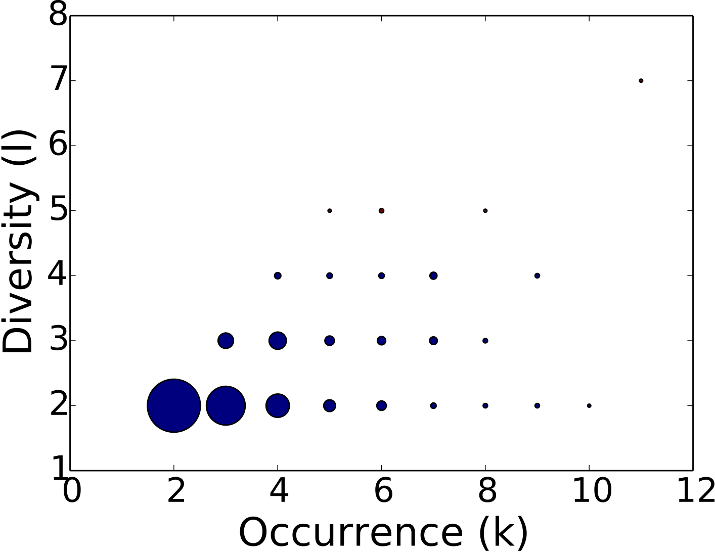
4.3.6 - value Distribution
Figure 14 shows the - value distribution of user pairs after spatial and temporal linkage. The usage ratio is taken as and the check-in probability is for this experiment. For a given pair in the results, we find the highest - diversity values it supports and maintain these counts. In the figure, the areas of the circles are proportional to number of pairs with the given - diversity. Since the number of pairs for - lower than - is too high (and precision very low as we have seen earlier), we do not present them in the results. As expected, the number of linked pairs is decreasing as the - values are increasing. It is interesting to note that for extreme values such as - diversity, it is still possible to find user pairs. We also observe that increasing diversity has a higher filtering power than increasing occurrence.
4.4 Integration with SERF
In addition to evaluating our approach under different settings, we also attempted to integrate our linkage model with the Stanford Entity Resolution Framework (SERF). SERF implements the R-Swoosh [4] algorithm. For this integration, users are arranged as entities and their events are considered as attributes. Given two entities, if they have enough number of co-occurring attributes satisfying the - diversity model, they are marked as a match.
Starting with pairwise comparison of entities, R-Swoosh algorithm gradually decreases the number of entities by merging the matching records, and deleting the dominated ones. While this is an effective method to decrease the number of comparisons on match heavy datasets, for datasets that contain few matching entities, the run-time is still . Merging of two records is valid only when there is merge associativity between records. Given three records, , , and , comparisons of and may result in different linkage decisions [3]. To alleviate this problem, the SERF framework also implements the Koosh algorithm [3]. Different than the R-Swoosh algorithm, when the Koosh algorithm finds a matching pair of entities, it does not merge them immediately, unless confidence is above a threshold. However, defining the confidence to use our spatio-temporal linkage model in SERF is not straightforward and requires further research, which we leave as future work.
Applying Koosh algorithm without using merges is almost brute force and using a small subset our dataset (15,268 users, 1,956,734 events, in total), SERF takes more than hours of processing time in the same setting. In comparison, our algorithm finds the matching users in the same dataset in minutes.
Summary
In this experimental study, we evaluated various aspects of the - diversity based linkage model and the ST-Link algorithm. We studied the scalability of the algorithm and showed that it scales linearly with the dataset size. We also studied the effectiveness of the linkage and showed that high precisions can be achieved. Using the unweighted version of our model, some of that precision can be traded off in order to achieve better recall values as well.
5 Related Work
Record Linkage.
One of the earliest appearances of the term record linkage is by
Newcombe et al. [28, 29]. Several surveys exist on the
topic [8, 13, 22]. Most of the work in this
area focus on a single type of databases and define the linked records with
respect to a similarity metric. The input to such a record linkage algorithm
is a set of records and the output from it is a clustering of records. In
contrast, our problem involves linking users from two datasets, where each
user can have multiple spatio-temporal records. A theoretical approach, and
its validation, on linking users across domains is studied
recently [31]. The first phase this work is computing a score
for every candidate pair. In a second phase they construct a bipartite graph
of users and reduce the problem into bipartite assignment problem. Their
experiments validate the accuracy of this two phase computation. While many
works on record linkage focus on accuracy [12, 5, 31]
and a few on scalability [36], our work must consider both. In our case,
successful linkage does not rely solely on the similarity of records and as
such ST-Link algorithm searches multiple diverse matches, aka -
diversity, and also makes sure that there are no negative matches, aka alibis.
To the best of our knowledge, this is a novel approach for record linkage,
specifically targeted at spatio-temporal datasets.
Temporal Record Linkage and Entity Evolution. Temporal record linkage
differs from traditional record linkage in that it takes entity evolution into
account (e.g., a person can change her phone number). The time decay
model captures the probability of an entity changing its attribute value
within a given time interval [24]. The mutation model
learns the probability of an attribute value re-appearing over
time [7]. The transition model learns the probability
of complex value transitions over time [23]. Furthermore,
declarative rules can be used to link records
temporally [6]. Transition model can also capture complex
declarative rules. Temporal record linkage algorithms are able to capture the
entity evolution and determine if an entity has changed the value of one or
more of its attributes. Our problem has some resemblance to entity evolution,
since the location attributes of the users change over time. However, this
change can be better described as entity mobility, rather than entity
evolution. Application of aforementioned models to spatio-temporal datasets
might be effective in predicting a user’s next stop or calculating the
probability of whether a user will return back to a given location. Yet, they
would fell short of linking spatio-temporal records of users.
Spatial Record Linkage and Spatial Joins. Many join and
self-join algorithms are proposed in the literature for spatial
data [21]. Sehgal et al. [34] proposes a
method to link the spatial records by integrating spatial and non-spatial
(e.g. location name) features. However, spatial record linkage and spatial
join algorithms are not extensible to spatio-temporal data as they are based
on intersection of minimum bounding boxes, one-sided nearest join, or string
similarity. Spatio-temporal joins are more complex with constrains on both
spatial and temporal domains [2]. Yet our problem involves more
than spatio-temporal records, it involves matching spatio-temporal record
series from two datasets.
Trajectory Join.
Bakalov et al. [1] define the trajectory joins as the
identification of all pairs of similar trajectories given two datasets. They
represent an object trajectory as a sequence of symbols. Based on the symbol
similarity, they prune the pairwise trajectory comparisons. Effective
evaluation of symbol similarity is supported by a tree-like index scheme.
In [2], the authors extend the problem to continuous queries over
streaming spatio-temporal trajectories. An important difference between
trajectory join algorithms and our work is that trajectory similarity is not
necessarily an indication of a linkage and vice verse. If one of the datasets
is denser than the other, trajectories would be dissimilar, yet we still can
have matching user pairs based on - linkage. However, some indexing
structures of trajectory join algorithms are closely related to our approach.
There are multiple indexing schemes for spatio-temporal data.
In [15, 27, 30, 26] various grid based
structures are used for indexing. Our spatial filtering approach is similar in
its use of a grid-based index, but instead of associating objects with grid
cells, we associate users with grid cells based on the frequency of their
events residing in these cells. There are also tree-like spatio-temporal
indexing structures, surveyed in [25]. A common theme of these
works is the reduction of the update cost, which is not a concern in our
work.
User Identification. Our work has
commonalities with the work done in the area of user identification. For
instance, de Montjoye et al. [10] has shown that, given a spatio-
temporal dataset of call detail records, one can uniquely identify the 95 %
of the population by using randomly selected spatio-temporal points. Similar to our
discussion, the authors mention that spatio-temporal points do not contribute
to information gain equally. In our work, we cover this by introducing a
weight function. Unlike our work, [10] does not consider
the linkage problem,
instead, they study how users can be uniquely identified within a single
dataset using a small subset of their records. Another related work
is [11], in which authors show that using the credit card
metadata, they can identify unique users and group the transactions with
respect to users. In addition to spatio-temporal reference data, they use the
transaction price and gender as auxiliary information. Another related work is
from Rossi et al. [32], in which user identification
techniques for GPS mobility data is presented. They
use a classification based algorithm rather than pairwise comparison of
records. Importantly, our
algorithm does not use any auxiliary information but only spatio-temporal
data, and it aims to match entities across datasets.
6 Conclusion
In this paper, we studied the problem of matching real-world entities using spatial-temporal usage records from two different LESs. By introducing the -–diversity model, a novel concept that captures both spatial and temporal diversity aspects of the linkage, we study the challenge of defining similarity between usage records of entities from different datasets. As part of this model, we introduced the concept of an alibi, which effectively filters out negative matches and significantly improves the linkage quality.
To realize the -–diversity model, we developed the scalable ST-Link algorithm that makes use of effective filtering steps. Taking advantage of the spatial nature of the data, users are associated with dominating grids — grids that contain most activities of their entities. This enables processing each grid independently, improving scalability. Taking advantage of the temporal nature of the data, we slide a window over both datasets jointly and maintain set of candidate users that have co-occurring events but no alibis. The set of candidate entities are pruned as the window is slided.
Our experimental evaluation, conducted with several data sets showed that the running time of the ST-Link algorithm scales linearly with the dataset size. Moreover, precision of the linkage results is practically for most - settings. We also observed that using an unweighted version of our linkage model, the precision can be sacrificed to achieve higher recall values.
Spatio-temporal linkage can enable gathering large dynamic data sets for many social good applications, such as smart cities and environmental monitoring. We are also investigating privacy preserving methodologies, those are needed to prevent information leakage while analyzing and sharing location based information [16, 38].
References
- [1] P. Bakalov, M. Hadjieleftheriou, E. Keogh, and V. J. Tsotras. Efficient trajectory joins using symbolic representations. In Int. Conf. on Mobile Data Management (MDM), pages 86–93, 2005.
- [2] P. Bakalov and V. Tsotras. Continuous spatiotemporal trajectory joins. In GeoSensor Networks, volume 4540 of Lecture Notes in Computer Science, pages 109–128. Springer Berlin Heidelberg, 2008.
- [3] O. Benjelloun, H. Garcia-Molina, H. Kawai, T. E. Larson, D. Menestrina, Q. Su, S. Thavisomboon, and J. Widom. Generic entity resolution in the serf project. Technical Report 2006-14, June 2006.
- [4] O. Benjelloun, H. Garcia-Molina, D. Menestrina, Q. Su, S. E. Whang, and J. Widom. Swoosh: A generic approach to entity resolution. The VLDB Journal, 18(1):255–276, Jan. 2009.
- [5] I. Bhattacharya and L. Getoor. Collective entity resolution in relational data. ACM TKDD, 1(1):5, 2007.
- [6] D. Burdick, M. A. Hernández, H. Ho, G. Koutrika, R. Krishnamurthy, L. Popa, I. Stanoi, S. Vaithyanathan, and S. R. Das. Extracting, linking and integrating data from public sources: A financial case study. IEEE Data Eng. Bull., 34(3):60–67, 2011.
- [7] Y.-H. Chiang, A. Doan, and J. F. Naughton. Modeling entity evolution for temporal record matching. In ACM Int. Conf. on Man. of Data, pages 1175–1186, 2014.
- [8] P. Christen. Data matching: concepts and techniques for record linkage, entity resolution, and duplicate detection. Springer Science & Business Media, 2012.
- [9] P. Christen and R. Gayler. Towards scalable real-time entity resolution using a similarity-aware inverted index approach. In Proc. of the 7th Australasian Data Mining Conf. - Volume 87, pages 51–60. Australian Computer Society, Inc., 2008.
- [10] Y.-A. de Montjoye, C. A. Hidalgo, M. Verleysen, and V. D. Blondel. Unique in the crowd: The privacy bounds of human mobility. Scientific reports, 3, 2013.
- [11] Y.-A. de Montjoye, L. Radaelli, V. K. Singh, et al. Unique in the shopping mall: On the reidentifiability of credit card metadata. Science, 347(6221):536–539, 2015.
- [12] X. Dong, A. Halevy, and J. Madhavan. Reference reconciliation in complex information spaces. In ACM Int. Conf. on Man. of Data, pages 85–96. ACM, 2005.
- [13] A. K. Elmagarmid, P. G. Ipeirotis, and V. S. Verykios. Duplicate record detection: A survey. IEEE TKDE, 19(1):1–16, 2007.
- [14] R. Finkel and J. Bentley. Quad trees a data structure for retrieval on composite keys. Acta Informatica, 4(1):1–9, 1974.
- [15] B. Gedik and L. Liu. Mobieyes: Distributed processing of continuously moving queries on moving objects in a mobile system. In Advances in Database Technology, volume 2992, pages 67–87. Springer Berlin Heidelberg, 2004.
- [16] B. Gedik and L. Liu. Protecting location privacy with personalized k-anonymity: Architecture and algorithms. IEEE Trans. on Mobile Computing, 7(1):1–18, 2008.
- [17] L. Getoor and A. Machanavajjhala. Entity resolution: Theory, practice & open challenges. In VLDB Conf., 2012.
- [18] S. Ghemawat and J. Dean. LevelDB. https://github.com/google/leveldb, 2015.
- [19] A. Gionis, P. Indyk, and R. Motwani. Similarity search in high dimensions via hashing. In VLDB Conf., pages 518–529. Morgan Kaufmann Publishers Inc., 1999.
- [20] M. A. Hernández and S. J. Stolfo. The merge/purge problem for large databases. In ACM Int. Conf. on Man. of Data, pages 127–138. ACM, 1995.
- [21] E. H. Jacox and H. Samet. Spatial join techniques. ACM Trans. Database Syst., 32(1), Mar. 2007.
- [22] H. Köpcke, A. Thor, and E. Rahm. Evaluation of entity resolution approaches on real-world match problems. Proc. of the VLDB Endowment, 3:484–493, Sept. 2010.
- [23] F. Li, M. L. Lee, W. Hsu, and W.-C. Tan. Linking temporal records for profiling entities. In ACM Int. Conf. on Man. of Data, pages 593–605. ACM, 2015.
- [24] P. Li, X. Dong, A. Maurino, and D. Srivastava. Linking temporal records. VLDB Conf., 4(11):956–967, 2011.
- [25] Y. Manolopoulos, Y. Theodoridis, and V. Tsotras. Spatiotemporal access methods. In Advanced Database Indexing, volume 17 of Advances in Database Systems, pages 141–166. Springer US, 2000.
- [26] M. F. Mokbel, X. Xiong, and W. G. Aref. Sina: Scalable incremental processing of continuous queries in spatio-temporal databases. In ACM Int. Conf. on Man. of Data, pages 623–634. ACM, 2004.
- [27] K. Mouratidis, D. Papadias, and M. Hadjieleftheriou. Conceptual partitioning: An efficient method for continuous nearest neighbor monitoring. In ACM Int. Conf. on Man. of Data, pages 634–645. ACM, 2005.
- [28] H. B. Newcombe and J. M. Kennedy. Record linkage: Making maximum use of the discriminating power of identifying information. Commun. ACM, 5(11):563–566, Nov. 1962.
- [29] H. B. Newcombe, J. M. Kennedy, S. J. Axford, and A. P. James. Automatic linkage of vital records: Computers can be used to extract ”follow-up” statistics of families from files of routine records. Science, 130(3381):954–959, 1959.
- [30] J. M. Patel, Y. Chen, and V. P. Chakka. Stripes: An efficient index for predicted trajectories. In ACM Int. Conf. on Man. of Data, pages 635–646. ACM, 2004.
- [31] C. Riederer, Y. Kim, A. Chaintreau, N. Korula, and S. Lattanzi. Linking users across domains with location data: Theory and validation. In Proc. of the Int. Conf.on WWW, pages 707–719, 2016.
- [32] L. Rossi, J. Walker, and M. Musolesi. Spatio-temporal techniques for user identification by means of GPS mobility data. CoRR, abs/1501.06814, 2015.
- [33] H. Samet, J. Sankaranarayanan, and M. Auerbach. Indexing methods for moving object databases: Games and other applications. In ACM Int. Conf. on Man. of Data, pages 169–180. ACM, 2013.
- [34] V. Sehgal, L. Getoor, and P. D. Viechnicki. Entity resolution in geospatial data integration. In Proc. of the 14th Annual ACM Int. Symp. on Adv. in Geographic Information Systems, pages 83–90, 2006.
- [35] A. Skovsgaard, D. Sidlauskas, and C. Jensen. Scalable top-k spatio-temporal term querying. In IEEE Int. Conf. on Data Engineering, pages 148–159, March 2014.
- [36] S. E. Whang and H. Garcia-Molina. Joint entity resolution on multiple datasets. The VLDB Journal, 22(6):773–795, 2013.
- [37] S. E. Whang, D. Marmaros, and H. Garcia-Molina. Pay-as-you-go entity resolution. IEEE TKDE, 25(5), 2013.
- [38] E. Yilmaz, H. Ferhatosmanoglu, E. Ayday, and R. C. Aksoy. Privacy-preserving aggregate queries for optimal location selection. IEEE Trans. on Dependable and Secure Computing, 1(1), 2017.
![[Uncaptioned image]](/html/1801.04101/assets/fuat.png) |
Fuat Basık is a graduate student in the Department of Computer Engineering, Bilkent University, Turkey. He holds a M.Sc. degree in Computer Science from Bilkent University. His research interests are in scalable data integration. |
![[Uncaptioned image]](/html/1801.04101/assets/bugra.png) |
Buğra Gedik is an Associate Professor in the Department of Computer Engineering, Bilkent University, Turkey. He holds a Ph.D. degree in Computer Science from Georgia Institute of Technology. His research interests are in data-intensive distributed systems. |
![[Uncaptioned image]](/html/1801.04101/assets/cagri.png) |
Çağrı Etemoğlu is a Manager at Turk Telekom. He holds a Ph.D. degree Electrical and Computer Engineering from University of California, Santa Barbara. His research interest is big data systems and applications. |
![[Uncaptioned image]](/html/1801.04101/assets/hakan.png) |
Hakan Ferhatosmanoğlu is a Professor in the Department of Science at the University of Warwick, and at Bilkent University. His research is on scalable data management and analytics for multi-dimensional data. He holds a Ph.D. degree in Computer Science from University of California, Santa Barbara. He received research career awards from the US Department of Energy, US National Science Foundation, The Science Academy of Turkey, and Alexander von Humboldt Foundation. |