21 cm Signal Recovery via the Robust Principle Component Analysis

Abstract

The redshifted 21 cm signal from neutral hydrogen (HI) is potentially a very powerful probe for cosmology, but a difficulty in its observation is that it is much weaker than foreground radiation from the Milky Way as well as extragalactic radio sources. The foreground radiation at different frequencies are however coherent along one line of sight, and various methods of foreground subtraction based on this property have been proposed. In this paper, we present a new method based on the Robust Principal Component Analysis (RPCA) to subtract foreground and extract 21 cm signal, which explicitly uses both the low-rank property of the frequency covariance matrix (i.e. frequency coherence) of the foreground and the sparsity of the frequency covariance matrix of the 21 cm signal. The low-rank property of the foregrounds frequency covariance has been exploited in many previous works on foreground subtraction, but to our knowledge the sparsity of the frequency covariance of the 21 cm signal is first explored here. By exploiting both properties in the RPCA method, in principle, the foreground and signal may be separated without the signal loss problem. Our method is applicable to both small patch of sky with the flat-sky approximation, and to large area of sky where the sphericity has to be considered. It is also easy to be extended to deal with more complex conditions such as sky map with defects.

I Introduction

Observation of the neutral hydrogen (HI) distribution through its 21 cm line radiation can provide very precious information on the history of the Epoch of Reionization (EoR) Furlanetto et al. (2006); Morales and Wyithe (2010); Pritchard and Loeb (2012); Zaroubi (2013) and the statistical properties of Large Scale Structure, which can be used to infer the nature of dark energy, dark matter, inflationary origin of the Universe Peterson et al. (2006); Chang et al. (2008); Ansari et al. (2008); Seo et al. (2010); Ansari et al. (2012). Detecting the 21 cm signal in a cosmological experiment is a very challenging task, because there are various astrophysical foreground emissions, such as galactic synchrotron emission, free-free emission, recombination lines, and the extragalactic radio sources including quasars, radio galaxies and galaxy clusters, some of these are several orders of magnitude stronger than the 21 cm signal. For example, for the intensity mapping (IM) experiment where the 21 cm signal intensity of the large scale structure is observed without resolving individual galaxies, the galactic synchrotron emission has $T_{b}\sim 10\,{\rm K}$ while the HI signal $T_{b}\sim$ a few $\,{\rm mK}$ at $z\sim 1$. To separate the the HI signal from the foreground components one has to use their distinct statistical characteristics.

The foreground spectra are expected to be smooth in the frequency domain, while the redshifted 21 cm signal fluctuates randomly at different frequencies. Early works demonstrated that the 21 cm signal can be successfully extracted from such foregrounds by low order polynomial fitting in image space spectra Wang et al. (2006); Jelić et al. (2008); Liu et al. (2009a), or alternatively in Fourier space Liu et al. (2009b), provided that the instrument response is smooth or well-known. However, in the real world the instrument responses are not smooth, and are only known up to the precision of calibration, which is itself a challenging task subject to many errors. More sophisticated methods which can deal with the non-smooth apparent foregrounds in the observational data are therefore developed. In the so called blind or semi-blind methods, no specific parametric model for the foregrounds is assumed, only generic features of the signal and foreground components such as their spectra smoothness and frequency coherence are used. Examples include the low-order polynomial fitting; Principle Component Analysis (PCA) or Singular Value Decomposition (SVD) Masui et al. (2013); Bigot-Sazy et al. (2015); Switzer et al. (2013, 2015) (to discriminate from the robust PCA method to be discussed below, we shall call it the classic PCA in the following); Independent Component Analysis (ICA) Chapman et al. (2012); Wolz et al. (2014); Alonso et al. (2015); and the Generalized Morphological Component Analysis (GMCA) Chapman et al. (2013), etc. However, so far the redshifted 21 cm signal has not yet been positively detected in the various EoR and IM experiments, it is imperative to improve these methods further and explore new approaches and methods .

In recent years, many powerful techniques and efficient algorithms in signal processing come out from the compressed sensing (CS) researches Candès et al. (2006); Donoho (2006), which offers a theoretical framework for simultaneously sensing and compressing finite dimensional vectors by linear dimensionality reduction. It shows that sparse or compressible signals can be recovered from highly incomplete measurements by using appropriate algorithms. The most prevalent structure used in CS is that of sparsity. Sparsity implies that the signal $x$ itself has only a small number of non-zero (or significantly non-zero in the case of not exactly sparse but compressible case) values, or $x$ can be sparsely represented in an appropriately chosen basis or frame. Another often pursuit structure is the low-rankness of matrices, where the rank is given by the number of non-zero singular values of the matrix. Low-rank approximation has many important applications for data compression, dimensionality reduction and so on in areas such as computer vision, information retrieval, and machine learning.

An important role in these developments is played by convex optimization Rockafellar (1970); Boyd and Vandenberghe (2004), which is a subfield of optimization, and has applications in a wide range of disciplines. The convexity makes the optimization easier than the general case since all its local minima must be global ones. Many compressive sensing problems can be formulated into an optimization problem, for example the most commonly encountered Basis Pursuit (BP) problem (also called the $l_{1}$ minimization problem) in compressive sensing

$$\min_{x}\,\mathinner{\!\left\lVert x\right\rVert}_{1}\qquad\text{subject to}\qquad y=Ax,$$ (1)

can be solved by an equivalent convex optimization problem

$$\min_{x}\,\mathinner{\!\left\lVert y-Ax\right\rVert}_{2}^{2}+\lambda\mathinner{\!\left\lVert x\right\rVert}_{1},$$ (2)

for some appropriate $\lambda>0$ (see the end of this section for notations). Because of the universality of the compressive sensing techniques and convex optimization methods, they found application in many areas, including astronomy and astrophysics Bobin et al. (2008). Some CS techniques have been applied to radio astronomy, mostly in interferometer array image synthesis Carrillo et al. (2013, 2014, 2015); Garsden et al. (2015); Girard et al. (2015); Ferrari et al. (2015); Onose et al. (2016a, b). In fact, even the classical Högbom CLEAN algorithm Högbom (1974) and its multi-scale version Wakker and Schwarz (1988) in radio image synthesis can be seen as matching pursuit algorithms from the CS perspective Lannes et al. (1997).

In this work, we introduce the Robust Principle Component Analysis (RPCA) method, which is a CS technique based on sparsity and low-rankness, to the problem of 21 cm signal and foregrounds separation. To our knowledge, this is the first conscious application of CS method in the 21 cm–foreground separation problem by taking advantage of the the sparsity and low-rank structure characteristics of the 21 cm signal and foregrounds frequency covariance information. It is also the first application of the RPCA method in 21cm foreground subtraction. While previous works has made use of the low- rank property of the foreground, the present work first exploited the sparsity of the 21cm signal.

The paper is organized as follows: We first describe the frequency covariance structure of the foregrounds and the 21 cm signal, and how the information of their distinct structures can be used to separate them from each other in subsection II.1 using the RPCA method. We introduce the RPCA method and the algorithm for its solution in subsection II.2, and show how this is done by a simulation in subsection II.3. Some details of the 21 cm signal and foreground simulation is given in Appendix A. We then introduce the generalized Internal Linear Combination (ILC) method to recovery the 21 cm signal from the extracted 21 cm signal frequency covariance matrix insection III, and compare the performance of our introduced method to that of the classical PCA method in section IV. Finally we discuss the results and its possible extensions in section V.

In this paper, we used various norms for vectors or matrices, for clarity, we summarize them here:

$\mathinner{\!\left\lVert\boldsymbol{x}\right\rVert}_{0}$

$l_{0}$-norm for vector or matrix $\boldsymbol{x}$, which is the number of non-zero elements of $\boldsymbol{x}$;

$\mathinner{\!\left\lVert\boldsymbol{x}\right\rVert}_{1}$

$l_{1}$-norm for vector $\boldsymbol{x}$, defined as $\mathinner{\!\left\lVert\boldsymbol{x}\right\rVert}_{1}\equiv\sum_{i}|x_{i}|$, if applied to a matrix the matrix is treated as a linear vector;

$\mathinner{\!\left\lVert\boldsymbol{x}\right\rVert}_{2}$

$l_{2}$-norm for vector $\boldsymbol{x}$, $\mathinner{\!\left\lVert\boldsymbol{x}\right\rVert}_{2}\equiv(\sum_{i}|x_{i}|^{2})^{1/2}$;

$\mathinner{\!\left\lVert\boldsymbol{x}\right\rVert}_{\infty}$

$l_{\infty}$-norm for vector $\boldsymbol{x}$, defined as $\mathinner{\!\left\lVert\boldsymbol{x}\right\rVert}_{\infty}\equiv\max|x_{i}|$, when applied to a matrix the matrix is treated as a linear vector;

$\mathinner{\!\left\lVert\boldsymbol{\mathbf{A}}\right\rVert}_{F}$

Frobenius norm for matrix $\boldsymbol{\mathbf{A}}$, a generalization of the $l_{2}$ norm for matrix, defined as $\mathinner{\!\left\lVert A\right\rVert}_{F}\equiv(\sum_{ij}A_{ij}^{2})^{1/2}$;

$\mathinner{\!\left\lVert\boldsymbol{\mathbf{A}}\right\rVert}_{*}$

Nuclear norm for matrix $\boldsymbol{\mathbf{A}}$ defined as the sum of its singular values. The nuclear norm can be interpreted as the $l_{1}$-norm of the vector of singular value of the matrix.

II The Robust PCA Method

II.1 Frequency Correlations

Consider a 21cm observation image data cube with two angular dimensions and one frequency dimension. The angular pixel indices are re-arranged as one index $p$, then the discrete multi-frequency sky maps is denoted as $x_{i}(p)$ at frequency $\nu_{i}$ and pixel $p$ as

$$x_{i}(p)=f_{i}(p)+s_{i}(p)+n_{i}(p),$$ (3)

where $f_{i}(p)$ is the foreground, $s_{i}(p)$ the HI 21 cm signal, and $n_{i}(p)$ the receiver noise contributions, or in vector form,

$$\boldsymbol{x}(p)=\boldsymbol{f}(p)+\boldsymbol{s}(p)+\boldsymbol{n}(p).$$ (4)

We assume that the 21 cm signal, astrophysical foreground and the instrument noise are uncorrelated with each other, and the noise in different frequency channels are independent and can be modeled as a zero-mean normal distribution, $n_{i}(p)\sim\mathcal{N}(0,\sigma_{i}^{2})$, where $\sigma_{i}^{2}$ is the variance of the noise in frequency channel $i$. Under this assumption, the $\nu-\nu^{\prime}$ covariance matrix of the noise will be a strictly diagonal matrix $\boldsymbol{\mathbf{N}}=\text{diag}\{\sigma_{1}^{2},\cdots,\sigma_{N_{\nu}}^{2}\}$. We have the $N_{\nu}\times N_{\nu}$ size $\nu-\nu^{\prime}$ covariance matrix of the observed data,

$$\boldsymbol{\mathbf{R}}=\frac{1}{N_{p}}\langle\boldsymbol{x}\boldsymbol{x}^{T}\rangle=\boldsymbol{\mathbf{R}}_{f}+\boldsymbol{\mathbf{R}}_{\text{HI}}+\boldsymbol{\mathbf{N}},$$ (5)

where $\boldsymbol{\mathbf{R}}_{f}$, $\boldsymbol{\mathbf{R}}_{\text{HI}}$ and $\boldsymbol{\mathbf{N}}$ are the $\nu-\nu^{\prime}$ covariance matrix of $\boldsymbol{f}$, $\boldsymbol{s}$ and $\boldsymbol{n}$, respectively, and the number of pixels $N_{p}$ is divided as an normalization factor to make the value of the elements of the covariance matrix roughly independent of pixelization. For a well constructed telescope system, to a first approximation, the frequency covariance matrix of the noise $\boldsymbol{\mathbf{N}}$ may be assumed as diagonal, i.e. the noise could be described by a white noise model, and the different frequency bins are uncorrelated. Such noise would be indistinguishable from that of the 21cm signal $\boldsymbol{\mathbf{R}}_{\text{HI}}$, as both are sparse and their non-zero elements concentrate on the diagonals. The noise in this case can be suppressed by longer integration time or by cross-correlating with other tracer signal (e.g. the galaxy density obtained by optical observations). If we know the variance of the noise $\sigma_{i}^{2}$ in each frequency bin, we could also subtract the frequency covariance matrix of the noise $\boldsymbol{\mathbf{N}}$ from $\boldsymbol{\mathbf{R}}$. In the following, to simplify the discussion, we shall not distinguish $\boldsymbol{\mathbf{N}}$ and $\boldsymbol{\mathbf{R_{\rm HI}}}$ any more, but treat them as an effective $\boldsymbol{\mathbf{R_{\rm HI}}}$, and solve the foregrounds and 21 cm signal separation problem

$$\boldsymbol{\mathbf{R}}=\boldsymbol{\mathbf{R}}_{f}+\boldsymbol{\mathbf{R}}_{\text{HI}}.$$ (6)

As radio point sources and diffuse foregrounds are all relatively smooth along frequency and have a long frequency coherence, their $\nu-\nu^{\prime}$ covariance is expected to have very low ranks. A way to see this is to note that $\boldsymbol{\mathbf{R}}_{f}$ can be expressed as

$$\boldsymbol{\mathbf{R}}_{f}=\frac{1}{N_{p}}\boldsymbol{\mathbf{M}}_{f}\boldsymbol{\mathbf{M}}_{f}^{T},$$

where $\boldsymbol{\mathbf{M}}_{f}$ is the $N_{\nu}\times N_{p}$ (foregrounds) sky data arranged as a matrix, and $\boldsymbol{\mathbf{M}}_{f}$ can be well modeled as a low-rank matrix. Its approximate SVD decomposition is

$$\boldsymbol{\mathbf{M}}_{f}\cong\boldsymbol{\mathbf{U}}\boldsymbol{\mathbf{\Sigma}}\boldsymbol{\mathbf{V}}^{T}=\sum_{i=1}^{r}\sigma_{i}\boldsymbol{u}_{i}\boldsymbol{v}_{i}^{*},$$

where $r\ll N_{\nu}$ is the rank of the matrix $\boldsymbol{\mathbf{M}}_{f}$, and $\sigma_{1}>\sigma_{2}>\cdots>\sigma_{r}$ are the non-zero singular values, and $\boldsymbol{\mathbf{U}}=[\boldsymbol{u}_{1},\cdots,\boldsymbol{u}_{r}]$, $\boldsymbol{\mathbf{V}}=[\boldsymbol{v}_{1},\cdots,\boldsymbol{v}_{r}]$ are the corresponding left and right singular vectors. This is the underlying principles of the classic PCA/SVD foreground subtraction method Masui et al. (2013); Alonso et al. (2015); Bigot-Sazy et al. (2015); Switzer et al. (2013, 2015).

On the other hand, the 21 cm signal has very short frequency coherence because its frequency corresponds directly to redshift and thus cosmic distance, its correlation diminishes as the frequency difference $\Delta\nu$ increases. The correlation length $\Delta\nu$ for the 21 cm signal also depends on the angular scale of observation, for the case of interest at $l\sim 100$, this signal is uncorrelated beyond $\Delta\nu\sim 1$ MHz or even less, while for $l\sim 10^{3}$ this occurs around $\sim 0.1$ MHz Bharadwaj and Ali (2005); Datta et al. (2007). For the 21 cm signal, the $\nu-\nu^{\prime}$ covariance matrix concentrates along the main diagonal, and the typical value of off-diagonal elements decay rapidly to essentially zero at a few MHz away. So the 21 cm $\nu-\nu^{\prime}$ covariance matrix is a very sparse one, especially in broad band observations, only elements along or near the diagonal have non-zero values.

II.2 The Algorithm

We see above that the $\nu-\nu^{\prime}$ covariance matrix of the foregrounds and 21 cm signal have distinctly different characteristics, the 21 cm signal has a very sparse structure, i.e., only elements along or near the the diagonal are non-zero, while the $\nu-\nu^{\prime}$ covariance matrix of foregrounds has low rank. Mathematically, separating such two components are exactly what the RPCA Candès et al. (2011); Wright et al. (2009); Chandrasekaran et al. (2011) is supposed to do, which tries to recover a low-rank component $L$ and a sparse component $S$ from their superposition $M=L+S$ under some suitable assumptions. In other words, the RPCA is to solve the problem

$$\min\ \text{rank}(L)+\lambda\mathinner{\!\left\lVert S\right\rVert}_{0}\quad\text{s.t.}\quad L+S=M,$$ (7)

over the (matrix) variables $L,S\in\mathbb{R}^{m\times n}$ and the regularization parameter $\lambda>0$. This is a non-convex problem, since the minimization of $\text{rank}(L)$ and $\mathinner{\!\left\lVert S\right\rVert}_{0}$ are non-convex and also NP-hard Natarajan (1995); Recht et al. (2010). Its convex relaxation is known as the Principal Component Pursuit (PCP), which is

$$\min\ \mathinner{\!\left\lVert L\right\rVert}_{*}+\lambda\mathinner{\!\left\lVert S\right\rVert}_{1}\quad\text{s.t.}\quad L+S=M,$$ (8)

where the nuclear norm $\mathinner{\!\left\lVert L\right\rVert}_{*}=\sum_{i}\sigma_{i}(L)$ is the sum of the singular values of the matrix, which is used as a convex proxy for the non-convex $\text{rank}(L)$, and the $l_{1}$-norm $\mathinner{\!\left\lVert S\right\rVert}_{1}=\sum_{ij}|S_{ij}|$ is used as a convex proxy for the non-convex $l_{0}$-norm $\mathinner{\!\left\lVert S\right\rVert}_{0}$. At first glance it may seem that for the PCP to work, one would have to choose a right regularization parameter $\lambda$, but in practice, the fixed choice $\lambda=1/\sqrt{\max{(m,n)}}$ works very well for almost all cases Candès et al. (2011). In this sense, there is no tunable parameter in the PCP problem.

Of course, in the most general case, there is an obvious degeneracy in the robust PCA problem Eq. (7) or its convex version – the PCP problem Eq. (8), i.e., how to distinguish $L$ and $S$ if both are sparse and have low ranks. To separate the two, we make the following assumptions on $L$ and $S$:

1. $L$ is not sparse or “spiky” in the basis we start with. This is imposed by requiring $L$ to be $\mu$-incoherent Candès and Recht (2008): given the SVD of the low-rank component (with rank $r$) $L=U\Sigma V^{*}$, let $U_{r}$ and $V_{r}$ denote the matrices consisting the first $r$ columns of $U$ and $V$ respectively, the incoherence parameter $\mu$ is a property of the matrix $L$, it is the smallest value that satisfies all the three inequalities Candès et al. (2011):

   $$\max_{i}\mathinner{\!\left\lVert U_{r}^{*}e_{i}\right\rVert}_{2}^{2} \leq \frac{\mu r}{m},$$ (9)

   $$\max_{i}\mathinner{\!\left\lVert V_{r}^{*}e_{i}\right\rVert}_{2}^{2} \leq \frac{\mu r}{n},$$ (10)

   $$\mathinner{\!\left\lVert U_{r}V_{r}^{*}\right\rVert}_{\infty} \leq \sqrt{\frac{\mu r}{mn}}.$$ (11)

   Satisfying the incoherence conditions means having a small value of $\mu$, this ensures that $L$ is not sparse Hornstein (2011).

2. The entries of $S$ are “spread out”, i.e. for $\alpha\in[0,1)$, we assume $S\in\mathcal{S}_{\alpha}$, where $\mathcal{S}_{\alpha}$ is defined as $\forall i\in[n],j\in[m]$,

   $$\mathcal{S}_{\alpha}\mathrel{\mathop{\mathchar 58\relax}}=\left\{A\in\mathbb{R}^{m\times n}\ \middle|\ \|A_{(i,\cdot)}\|_{0}\leq\alpha n,\|A_{(\cdot,j)}\|_{0}\leq\alpha m\right\}\\$$

   In other words, $S$ contains at most a fraction $\alpha$ of non-zero entries per row and column. This guarantees that the probability of $S$ be low-rank is small. For example, if the non-zero elements of $A$ are mainly concentrate on the diagonal, as the case of the frequency covariance matrix of the 21 cm signal we are discussing it satisfies the condition $\mathcal{S}_{\alpha}$.

The frequency covariance of the foregrounds is low-rank but not sparse, satisfying condition 1; and the frequency covariance matrix of the 21 cm signal is sparse but not low-rank, satisfying condition 2. Under such assumptions, the PCP problems is solvable and convergence guaranteed (c.f. Theorem 1.1 of Candès et al. (2011)).

The PCP problem is a convex optimization problem, many off-the-shelf algorithms and tools are available for its solution Liu and Vandenberghe (2009); Mohan and Fazel (2012); Boyd et al. (2003); Lin et al. (2009); Eckstein and Yao (2012); Boyd et al. (2011). New algorithm customized for the RPCA and the PCP problem have also been developed, which are generally faster, more robust to corruptions or outliers, or more scalable for large problems Lin et al. (2010); Netrapalli et al. (2014); Kang et al. (2015); Yi et al. (2016). Here we use an augmented Lagrange multiplier (ALM) algorithm Lin et al. (2010); Yuan and Yang (2009) to solve the PCP problem Eq.(8), which is faster and more accurate than, e.g., the Accelerated Proximal Gradient (APG) method Lin et al. (2009). The ALM method operates on the augmented Lagrangian

$$l(L,S,Y) = \mathinner{\!\left\lVert L\right\rVert}_{*}+\lambda\mathinner{\!\left\lVert S\right\rVert}_{1}+\langle Y,M-L-S\rangle$$ (12)

$$+ \frac{\mu}{2}\mathinner{\!\left\lVert M-L-S\right\rVert}_{F}^{2},$$

where $Y$ is an Lagrange multiplier matrix and $\mu$ is a positive scalar. A generic Lagrange multiplier algorithm would solve the PCP problem by repeatedly setting

$$(L_{k},S_{k})=\text{arg}\,\min_{L,S}\,l(L,S,Y_{k})$$ (13)

and then updating the Lagrange multiplier matrix via

$$Y_{k+1}=Y_{k}+\mu(M-L_{k}-S_{k}).$$

Two ALM methods had been proposed to solve the RPCA problemLin et al. (2010): the exact ALM (EALM) method has a pleasing Q-linear convergence speed, and a slight improvement over the exact ALM leads an inexact ALM (IALM) method, which converges practically as fast as the exact ALM, but the required number of partial SVDs is significantly less. Here, we will use the IALM method, since the algorithm is easy to implement, and performs excellently on a wide range of problem settings without need of tuning parameters.

The IALM method does not solve Eq. (12) exactly, rather, it alternately updates $L_{k}$ and $S_{k}$ by solving a sequence of convex programs of $\text{min}_{L}\,l(L,S,Y)$ and $\text{min}_{S}\,l(L,S,Y)$ while keeping the other matrix variables fixed. By doing so, both problems have very simple and efficient closed solutions. Let $\mathcal{S}_{\tau}\mathrel{\mathop{\mathchar 58\relax}}\mathbb{R}\to\mathbb{R}$ denote the shrinkage operator (also called the soft-thresholding operator),

$$\mathcal{S}_{\tau}[x]=\text{sgn}(x)\,\text{max}(|x|-\tau,0),$$

and extend it to matrices by applying it to each element. It is easy to show that the solution to the first problem is

$$\text{arg}\,\min_{S}\,l(L,S,Y)=\mathcal{S}_{\lambda\mu^{-1}}(M-L+\mu^{-1}Y).$$ (14)

Similarly, for matrix $X$, let $\mathcal{D}_{\tau}(X)$ denote the singular value thresholding operator given by Cai et al. (2010)

$$\mathcal{D}_{\tau}(X)=U\mathcal{S}_{\tau}(\Sigma)V^{*},$$

where $X=U\Sigma V^{*}$ is its singular value decomposition, it can be shown that

$$\text{arg}\,\min_{L}\,l(L,S,Y)=\mathcal{D}_{\mu^{-1}}(M-L+\mu^{-1}Y).$$ (15)

The above method is summarized in Algorithm 1, proof of its convergence is given in Lin et al. (2010). The iteration of the algorithm can be stopped once

$$\mathinner{\!\left\lVert M-L-S\right\rVert}_{F}\leq\delta\mathinner{\!\left\lVert M\right\rVert}_{F},$$ (16)

with a sufficiently small $\delta$, where the Frobenius norm $\mathinner{\!\left\lVert M\right\rVert}_{F}^{2}=\sum_{ij}M_{ij}^{2}.$

Algorithm 1 (The PCP problem by ALM)

1:  initialize: $S_{0}=Y_{0}=0,\mu>0,\delta>0$.

2:  while $\mathinner{\!\left\lVert M-L-S\right\rVert}_{F}>\delta\mathinner{\!\left\lVert M\right\rVert}_{F}$  do

3:        compute $L_{k+1}=\mathcal{D}_{\mu}^{-1}(M-S_{k}+\mu^{-1}Y_{k})$;

4:        compute $S_{k+1}=\mathcal{S}_{\lambda\mu^{-1}}(M-L_{k+1}+\mu^{-1}Y_{k})$;

5:        compute $Y_{k+1}=Y_{k}+\mu(M-L_{k+1}-S_{k+1})$;

6:  end while

7:  output: $L,S$.

In the problem of foregrounds and 21 cm signal component separation, as discussed above, the assumption that the low-rank component (the frequency covariance matrix of the foregrounds) is not “spiky” and the entries of the sparse one (the frequency covariance matrix of the 21 cm signal) are “spread out” is obviously satisfied. In contrast to the usual application of the RPCA method and the PCP problem where recovery of the low rank matrix $L$ is the primary goal, here the sparse component $S$ is what we really want, as it will provide a good estimate for the HI 21 cm frequency covariance matrix $\boldsymbol{\mathbf{\hat{R}}}_{\text{HI}}$. The low rank component $L$ may also be of interest as it gives a good approximation of the foreground frequency covariance matrix $\boldsymbol{\mathbf{\hat{R}}}_{f}$, which as a byproduct, actually provides an estimate of the foreground from the observation itself. Note that the matrix $\boldsymbol{\mathbf{R}}$ is symmetric positive definite in this problem, as it is the frequency covariance matrix of the observed sky, but the RPCA method and the PCP algorithm do not require this, the matrix $M$ in Eqs.(7) or (8) can be non-symmetric, so the same method can be applied in the case of cross-correlation with other observation, and even non-square matrix in the general case.

Figure 1: Input sky maps at 750 MHz. From left to right, top to bottom, the brightness temperature of the simulated Galactic synchrotron emission, 21 cm signal, extragalactic point sources and the sum of the three components, respectively. To better visualize the point source, in the bottom left panel a small part of the map, ($-15\degree\leq\alpha\leq 15\degree$, $-10\degree\leq\delta\leq 10\degree$), is shown .

For comparison, the frequently used classical PCA can be expressed as solving the (non-convex) problem

$$\min\,\mathinner{\!\left\lVert M-L\right\rVert}_{F}\quad\text{s.t.}\quad\text{rank}(L)\leq k,$$ (17)

with problem data $M$, variable $L$, and integer $k\geq 1$. In the classical PCA, $M$ is approximated as a low rank matrix $L$ with the Frobenius norm error minimized. It can be efficiently solved with the SVD method, and works well when the error is small and distributed as independent and identically Gaussian. But the classical PCA is not robust when the data is grossly corrupted, i.e., with large outliers. Also it is easy to fail in cases when a matrix is only a few sparse terms away from being low-rank, especially if the sparse terms have large magnitudes. By contrast, RPCA decomposes a matrix into the sum of a low-rank matrix and a sparse matrix, thereby separates out the sparse errors, the entries in the sparse error matrix $S$ can have arbitrary large magnitude as long as its support is sufficiently small. Performing this separation prevents the sparse errors from obscuring the low-rank component Candès et al. (2011).

II.3 Simulation

Figure 2: Frequency correlation matrix of data $\boldsymbol{\mathbf{R}}$ (upper left), the recovered low-rank matrix $L$ (lower left) and the sparse matrix $S$ (lower right), and the difference of $\boldsymbol{\mathbf{R}}_{\text{HI}}-S$ (upper right).

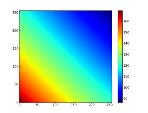
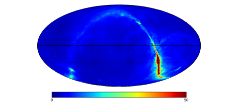
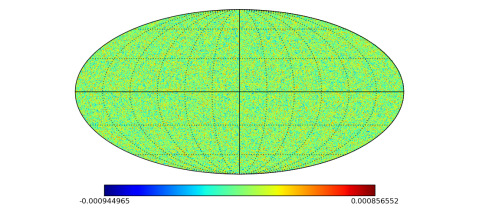
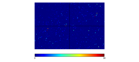
We use simulated sky map data to demonstrate the application of the RPCA method for the separation of the foregrounds and the 21 cm signal. The real foreground may consist of many different physical components, such as synchrotron radiation, free-free emission, and emission by dusts. Here for demonstration we only include the two main components at low frequencies, i.e. the galactic synchrotron radiation and the extragalactic radio point sources. For this simulation, we use the Cosmology in the Radio Band (CORA)  Shaw et al. (2014, 2015) package, which simulates sky emission including galactic and extragalactic foregrounds, with some extra utility codes for dealing with Healpix maps and spherical co-ordinates. We consider a case which is inspired by the Tianlai experiment Chen (2012) whose pathfinder works at the frequency range $700-800\,{\rm MHz}$. We generate the sky maps in the frequency range $700-800$ MHz, with 256 equally spaced frequency bins ($\Delta\nu\sim 0.39$ MHz), and the whole sky is divided using the HEALPix pixelization scheme Górski et al. (2005) with $n_{\text{side}}=256$, which corresponds to an angular resolution of $\sim 13.7$ arcmin. To take the effect of frequency dependent beam into account, we first convolve the generated sky maps with a symmetric circular frequency dependent Gaussian beam with $\theta=1.22\lambda/D$, where $\lambda$ is the observing wavelength, and $D$ is the diameter of the telescope. We take $D=100$m, corresponding to the optimal size for the mid-redshift 21cm intensity mapping experiment Chang et al. (2008); Seo et al. (2010); Ansari et al. (2012), and also the size of current largest fully steerable telescope, such as the Green Bank Telescope (GBT) which is conducting intensity mapping observations Chang et al. (2010); Masui et al. (2013); Switzer et al. (2013). For this size the beam width is $\sim 16.8$ arcmin at 750 MHz, which roughly matches the resolution of the map. The details of the simulation is given in Appendix A. We tested our procedure by making 10 different realizations of the random field, and found similar results in each case. One of these is shown in Figure 1, at the central frequency of 750 MHz.

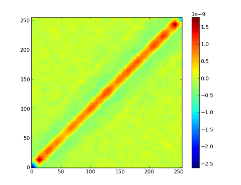
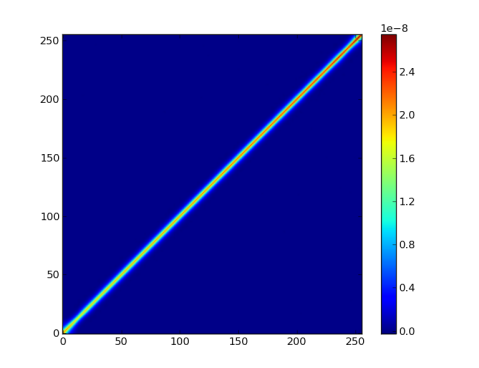
We use Algorithm 1 to solve the PCP problem, with a fixed regularization parameter $\lambda=1/\sqrt{N_{\nu}}$, where $N_{\nu}$ is the number of rows (or columns) of the $\nu-\nu^{\prime}$ covariance matrix $\boldsymbol{\mathbf{R}}$. After a few trials, we found that $\mu=10^{8}$ works, though it is not necessarily the optimal value. We terminate the algorithm when $\mathinner{\!\left\lVert\boldsymbol{\mathbf{R}}-L-S\right\rVert}_{F}\leq\delta\,\mathinner{\!\left\lVert\boldsymbol{\mathbf{R}}\right\rVert}_{F}$ with $\delta=10^{-14}$. The algorithm converges quickly with this choice of $\lambda$ and $\mu$, it takes less than 100 iterations to get the required precision. The frequency covariance matrix $\boldsymbol{\mathbf{R}}$ is then successfully decomposed into a low-rank component $L$, which is mainly the contribution of the foreground, and an almost diagonal sparse component $S$, which represents the frequency covariance matrix of the 21 cm signal. The result is shown in Figure 2, from which we see the maximum element difference between $S$ and the input $\boldsymbol{\mathbf{R}}_{\text{HI}}$ is at least an order of magnitude lower than the corresponding element of $\boldsymbol{\mathbf{R}}_{\text{HI}}$, shown a very accurate recovery of the 21 cm signal frequency covariance matrix from the total signal.

III 21cm Signal Recovery

Once we obtained the 21 cm $\nu-\nu^{\prime}$ covariance matrix $\boldsymbol{\mathbf{\hat{R}}}_{\text{HI}}$ (the sparse matrix $S$) and the foreground covariance matrix $\boldsymbol{\mathbf{\hat{R}}}_{f}$ (the low-rank matrix $L$), the 21cm signal can be recovered from the data. A number of methods are available for this task, some by using only $S$, and others may use both $L$ and $S$. For example, the Karhunen-Loève (K-L) transform method is one of the latter, it seeks to find a linear transformation of the observed data $\boldsymbol{x}^{\prime}=\boldsymbol{\mathbf{P}}\boldsymbol{x}$ such that by projecting onto the transformation matrix $\boldsymbol{\mathbf{P}}$ the signal covariance matrix $S$ becomes diagonal and the noise (here the foreground) covariance matrix $L$ becomes the identity matrix $\boldsymbol{\mathbf{I}}$:

$$S\to S^{\prime} =\boldsymbol{\mathbf{P}}S\boldsymbol{\mathbf{P}}^{T}=\boldsymbol{\mathbf{\Lambda}},$$

$$L\to L^{\prime} =\boldsymbol{\mathbf{P}}L\boldsymbol{\mathbf{P}}^{T}=\boldsymbol{\mathbf{I}},$$ (18)

where $\boldsymbol{\mathbf{\Lambda}}$ is a diagonal matrix, and $\boldsymbol{\mathbf{I}}$ is the identity matrix. The sub-space with low foreground contamination can then be identified as those with larger values of diagonal elements of $\boldsymbol{\mathbf{\Lambda}}$. Mathematically, this transformation can be found by solving the generalized eigenvalue problem $S\boldsymbol{x}=\lambda L\boldsymbol{x}$, or written in matrix form $S\boldsymbol{\mathbf{X}}=L\boldsymbol{\mathbf{X}}\boldsymbol{\mathbf{\Lambda}}$. This gives a set of eigenvectors $\boldsymbol{x}$ (or $\boldsymbol{\mathbf{X}}$), and corresponding eigenvalues $\lambda$ (or $\boldsymbol{\mathbf{\Lambda}}$), then $\boldsymbol{\mathbf{X}}=\boldsymbol{\mathbf{P}}^{T}$, i.e. the transformation matrix $\boldsymbol{\mathbf{P}}$ consists each eigenvectors $\boldsymbol{x}$ as a row. To recover the 21 cm signal, select modes with eigenvalue (which is the signal-to-foreground power) greater than a certain threshold. Define the matrix $\boldsymbol{\mathbf{P}}_{s}$ which contains only the rows from $\boldsymbol{\mathbf{P}}$ corresponding to eigenvalues greater than the threshold $s$, the 21 cm signal is then recovered approximately by $\boldsymbol{\hat{s}}=\boldsymbol{\mathbf{P}}_{s}\boldsymbol{x}$.

This 21 cm signal recovery method depends on the joint transformation of $L$ and $S$, the inaccuracy in either $L$ and $S$ may lead to large errors. Another potential problem of this method is that for the generalized eigenvalue problem to have a solution, $L$ must be symmetric positive definite, but there is no guarantee for this in the RPCA decomposition, and the solution would fail if $L$ is not positive definite. For these reasons, here we choose to uses only the $S$ matrix, which is generally more robust than methods which depend on both $L$ and $S$. Note that to do RPCA decomposition, both the sparsity of $S$ and low-rank of $L$ and needed, but to recover the 21 cm signal, $S$ is sufficient.

In this paper we use the generalized Internal Linear Combination (ILC) method Remazeilles et al. (2011) to recover the 21 cm signal. The ILC component separation method has been extensively used to extract the cosmic microwave background (CMB) from the WMAP multi-frequency data Bennett et al. (2003); Tegmark et al. (2003); Delabrouille et al. (2009). However, here we will follow the method and symbol notations presented in Olivari et al. (2016) because which also deals with HI signal extraction, thus closer to our work.

We have already mentioned that foreground components are correlated over frequencies, so we expect that the foregrounds signal can be represented as a linear combination of a finite number $m$ of independent templates, which do not necessarily represent physical components. In other words, we try to capture all foreground contributions as resulting from $m$ (unphysical) templates, so $m$ is just the effective dimension of the foregrounds subspace. While the 21 cm signal $\boldsymbol{s}$ is only correlated over adjacent frequencies, and can be represented as the linear combination of $N_{\nu}-m$ independent (unphysical) templates $\boldsymbol{t}$,

$$\boldsymbol{s}=\boldsymbol{\mathbf{S}}\boldsymbol{t},$$ (19)

where $\boldsymbol{\mathbf{S}}$ is a $N_{\nu}\times(N_{\nu}-m)$ mixing matrix giving the contribution from the templates to the HI emission in each frequency channel. Note that we are not interested in recovering $\boldsymbol{t}$, our goal is just to use it to explore the subspace of the HI signal and recover $\boldsymbol{s}$. Using this expression, we can write the 21 cm $\nu-\nu^{\prime}$ covariance matrix as

$$\boldsymbol{\mathbf{R}}_{\text{HI}}=\boldsymbol{\mathbf{S}}\boldsymbol{\mathbf{R}}_{t}\boldsymbol{\mathbf{S}}^{T},$$ (20)

where $\boldsymbol{\mathbf{R}}_{t}=\langle\boldsymbol{t}\boldsymbol{t}^{T}\rangle$ is the $(N_{\nu}-m)\times(N_{\nu}-m)$ covariance matrix of the templates $\boldsymbol{t}$. The generalized ILC method estimates the signal $\boldsymbol{s}$ as a linear combination of the total signal $\boldsymbol{x}$ as

$$\hat{\boldsymbol{s}}=\boldsymbol{\mathbf{W}}\boldsymbol{x},$$ (21)

where $\boldsymbol{\mathbf{W}}$ is the $N_{\nu}\times N_{\nu}$ ILC weight matrix, which have unit response to the 21 cm signal, while minimizing the total variance of the vector estimate $\hat{\boldsymbol{s}}$. The optimal weighting matrix of the generalized multi-dimensional ILC can be written as Remazeilles et al. (2011)

$$\boldsymbol{\mathbf{W}}=\boldsymbol{\mathbf{S}}(\boldsymbol{\mathbf{S}}^{T}\boldsymbol{\mathbf{R}}^{-1}\boldsymbol{\mathbf{S}})^{-1}\boldsymbol{\mathbf{S}}^{T}\boldsymbol{\mathbf{R}}^{-1}.$$ (22)

We can see from Eq. (22) that $\boldsymbol{\mathbf{W}}$ is invariant under the transformation $\boldsymbol{\mathbf{S}}\to\boldsymbol{\mathbf{S}}\boldsymbol{\mathbf{T}}$ for any invertible matrix $\boldsymbol{\mathbf{T}}$, so $\boldsymbol{t}$ can also be replaced by any other linear combination $\boldsymbol{\mathbf{T}}\boldsymbol{t}$. We apply the following transformation to the total signal $\boldsymbol{x}$ using the estimated 21 cm $\nu-\nu^{\prime}$ covariance matrix $\boldsymbol{\mathbf{\hat{R}}}_{\text{HI}}$,

$$\boldsymbol{x}\to\boldsymbol{\mathbf{\hat{R}}}_{\text{HI}}^{-1/2}\boldsymbol{x},$$ (23)

where the matrix $\boldsymbol{\mathbf{\hat{R}}}_{\text{HI}}^{-1/2}$ is defined to satisfy $\boldsymbol{\mathbf{\hat{R}}}_{\text{HI}}^{-1/2}\boldsymbol{\mathbf{\hat{R}}}_{\text{HI}}\boldsymbol{\mathbf{\hat{R}}}_{\text{HI}}^{-1/2}=\boldsymbol{\mathbf{I}}$, and can be calculated by eigen-decomposition: $\boldsymbol{\mathbf{\hat{R}}}_{\text{HI}}=\boldsymbol{\mathbf{U}}\boldsymbol{\mathbf{\Lambda}}\boldsymbol{\mathbf{U}}^{T}$, then $\boldsymbol{\mathbf{\hat{R}}}_{\text{HI}}^{-1/2}=\boldsymbol{\mathbf{U}}\boldsymbol{\mathbf{\Lambda}}^{-1/2}\boldsymbol{\mathbf{U}}^{T}$.

Figure 3: Eigen-values of the covariance matrix $\boldsymbol{\mathbf{C}}=\boldsymbol{\mathbf{\hat{R}}}_{\text{HI}}^{-1/2}\boldsymbol{\mathbf{R}}\boldsymbol{\mathbf{\hat{R}}}_{\text{HI}}^{-1/2}$. Top is for the parameters setting of this simulation, four eigen-values are significantly larger; bottom is for the case when the 21 cm signal is 1000 times larger, now there is two significantly lager eigen-values.

Table 1: The largest 20 eigenvalues.

$2.680\times 10^{11}$	$2.187\times 10^{8}$	$3.751\times 10^{4}$	$3.824\times 10^{1}$	1.201
1.188	1.181	1.169	1.164	1.147
1.135	1.129	1.119	1.108	1.099
1.089	1.082	1.073	1.063	1.055

The transformed quantity $\boldsymbol{\mathbf{\hat{R}}}_{\text{HI}}^{-1/2}\boldsymbol{x}$ will have a covariance

$$\boldsymbol{\mathbf{C}} \equiv \boldsymbol{\mathbf{\hat{R}}}_{\text{HI}}^{-1/2}\boldsymbol{\mathbf{R}}\boldsymbol{\mathbf{\hat{R}}}_{\text{HI}}^{-1/2}$$ (24)

$$= \boldsymbol{\mathbf{\hat{R}}}_{\text{HI}}^{-1/2}\boldsymbol{\mathbf{R}}_{f}\boldsymbol{\mathbf{\hat{R}}}_{\text{HI}}^{-1/2}+\boldsymbol{\mathbf{\hat{R}}}_{\text{HI}}^{-1/2}\boldsymbol{\mathbf{R}}_{\text{HI}}\boldsymbol{\mathbf{\hat{R}}}_{\text{HI}}^{-1/2}.$$

The estimated HI $\nu-\nu^{\prime}$ covariance matrix $\boldsymbol{\mathbf{\hat{R}}}_{\text{HI}}$ is close to the real HI covariance matrix $\boldsymbol{\mathbf{R}}_{\text{HI}}$, so the last term in Eq. (24) will be close to the identity matrix $\boldsymbol{\mathbf{I}}$. Now if we make an eigen-decomposition of the left covariance matrix of Eq. (24), we have

$$\boldsymbol{\mathbf{C}}=[\boldsymbol{\mathbf{U}}_{F}\boldsymbol{\mathbf{U}}_{S}]\times\begin{bmatrix}\lambda_{1}+1&&&\\ &\cdots&&\\ &&\lambda_{m}+1&\\ &&&\boldsymbol{\mathbf{\tilde{I}}}\\ \end{bmatrix}\,\times\,\begin{bmatrix}\boldsymbol{\mathbf{U}}_{F}^{T}\\ \boldsymbol{\mathbf{U}}_{S}^{T}\end{bmatrix},$$ (25)

where $\boldsymbol{\mathbf{\tilde{I}}}$ is used to denote the appropriate identity sub-matrix. From this we see that the eigenvalues of the covariance matrix $\boldsymbol{\mathbf{C}}=\boldsymbol{\mathbf{\hat{R}}}_{\text{HI}}^{-1/2}\boldsymbol{\mathbf{R}}\boldsymbol{\mathbf{\hat{R}}}_{\text{HI}}^{-1/2}$ that are nearly unity contains the power of the HI 21 cm signal, with the corresponding eigenvectors spanning the HI subspace. This is equivalent to say that the eigenvalues significantly greater than unity contains the foreground components, and the number of these eigenvalues determines $m$, the dimension of foreground subspace.

We can extract the subspace corresponding to the HI 21 cm signal as

$$\boldsymbol{\mathbf{\hat{R}}}_{\text{HI}}^{-1/2}\boldsymbol{\mathbf{R}}_{\text{HI}}\boldsymbol{\mathbf{\hat{R}}}_{\text{HI}}^{-1/2}=\boldsymbol{\mathbf{U}}_{S}\,\boldsymbol{\mathbf{\tilde{I}}}\,\boldsymbol{\mathbf{U}}_{S}^{T},$$ (26)

which can be re-written as

$$\boldsymbol{\mathbf{R}}_{\text{HI}}=\boldsymbol{\mathbf{\hat{R}}}_{\text{HI}}^{1/2}\boldsymbol{\mathbf{U}}_{S}\,\boldsymbol{\mathbf{\tilde{I}}}\,\boldsymbol{\mathbf{U}}_{S}^{T}\boldsymbol{\mathbf{\hat{R}}}_{\text{HI}}^{1/2}.$$ (27)

This is just the $N_{\nu}\times N_{\nu}$ HI $\nu-\nu^{\prime}$ covariance matrix projected onto the $(N_{\nu}-m)$-dimensional HI subspace spanned by the subset of eigenvectors collected in matrix $\boldsymbol{\mathbf{U}}_{S}$. Compare Eq. (27) with Eq. (20), and using the fact that the template $\boldsymbol{t}$ can be replaced by any linear combination $\boldsymbol{\mathbf{T}}\boldsymbol{t}$ provided $\boldsymbol{\mathbf{T}}$ is invertible, we can choose $\boldsymbol{\mathbf{T}}$ to be the orthogonal transform matrix of $\boldsymbol{\mathbf{R}}_{t}$ to re-express Eq. (20) as

$$\boldsymbol{\mathbf{R}}_{\text{HI}}=\boldsymbol{\mathbf{S}}\boldsymbol{\mathbf{T}}\boldsymbol{\mathbf{D}}_{t}\boldsymbol{\mathbf{T}}^{T}\boldsymbol{\mathbf{S}}^{T},$$ (28)

where $\boldsymbol{\mathbf{D}}_{t}$ is the diagonal matrix of the orthogonal transform $\boldsymbol{\mathbf{R}}_{t}=\boldsymbol{\mathbf{T}}\boldsymbol{\mathbf{D}}_{t}\boldsymbol{\mathbf{T}}^{T}$. Now we can see that

$$\boldsymbol{\mathbf{S}}\boldsymbol{\mathbf{T}}=\boldsymbol{\mathbf{\hat{R}}}_{\text{HI}}^{1/2}\boldsymbol{\mathbf{U}}_{S}$$ (29)

up to an scaling factor which could be absorbed into $\boldsymbol{\mathbf{T}}$. Since $\boldsymbol{\mathbf{W}}$ is invariant under the transform of $\boldsymbol{\mathbf{S}}\to\boldsymbol{\mathbf{S}}\boldsymbol{\mathbf{T}}$ for any invertible matrix $\boldsymbol{\mathbf{T}}$, we get the estimate of the mixing matrix of the 21 cm signal as

$$\boldsymbol{\mathbf{\hat{S}}}=\boldsymbol{\mathbf{\hat{R}}}_{\text{HI}}^{1/2}\boldsymbol{\mathbf{U}}_{S}.$$ (30)

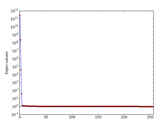
Now we can substitute Eq. (30) into Eq. (22), then from Eq. (21) we can get the recovered HI 21 cm signal. We show that the eigenvalues of the covariance matrix $\boldsymbol{\mathbf{C}}$ for the simulated data in Figure 3 and the largest 20 eigen-values in Table 1.

Figure 4: HI 21 cm signal recovery result for a threshold 2.0. Subfigures are: (a) the recovered 21 cm signal, (b) the relative difference of the input 21 cm signal and the recovered 21 cm signal.

Figure 5: The normalized angular power spectrum $l(l+1)C_{l}/2\pi$ of the recovered HI 21 cm signal for a threshold 2.0 (top), where the curve labeled “cross” is the cross angular power spectrum of the input 21 cm signal and the recovered 21 cm signal, and the transfer function $T_{l}=C_{l}^{\text{input}}/C_{l}^{\text{recovered}}$ (bottom).

From Eq. (25) we see the eigenvalues of $\boldsymbol{\mathbf{C}}$ are $1+\lambda_{m}$, so if we select $\lambda_{m}>1$ or the eigenvalues of $\boldsymbol{\mathbf{C}}$ greater than 2, the subspace of the eigenvectors would correspond to the low rank matrix $\boldsymbol{\mathbf{L}}$, so in fact there is no arbitrary choice here. From Figure 3 and Table 1, we see that in this simulation there are four large eigenvalues, all other eigenvalues are significantly smaller. As we will see, this number is also the optimal number of eigen-modes that should be subtracted in the classic PCA method, which actually reflects the fact that our foreground model has four principal components that dominates the 21 cm signal. We have also made tests to check this correspondence. For example, if we artificially increase the 21 cm signal by 1,000 times while keeping the foregrounds unchanged, now the signal actually dominates the smaller two principal components of the foregrounds, and we see there is only two eigenvalues that are significantly larger as shown in the bottom of Figure 3. The GILC method can quite automatically and robustly detected the dimensionality of the foreground subspace, which is an additional advantage of our method against the classic PCA method we will discuss next.

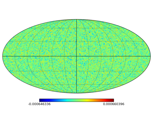
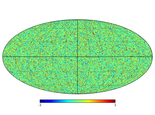
We show in Fig.4 (a) the recovered 21 cm signal, (b) the relative difference of the input 21 cm signal and the recovered 21 cm $(\boldsymbol{x}^{\text{recovered}}-\boldsymbol{x}^{\text{input}})/(\bar{T}_{b}+\boldsymbol{x}^{\text{input}})$, where $\bar{T}_{b}$ is the mean temperature of the 21 cm signal computed according to Equation 35. For fully accurate recover, the relative difference is 0. We can see from the figure that the signal is generally well recovered, as most points of the map the relative error is nearly zero. The residue deviations are randomly distributed over the sky.

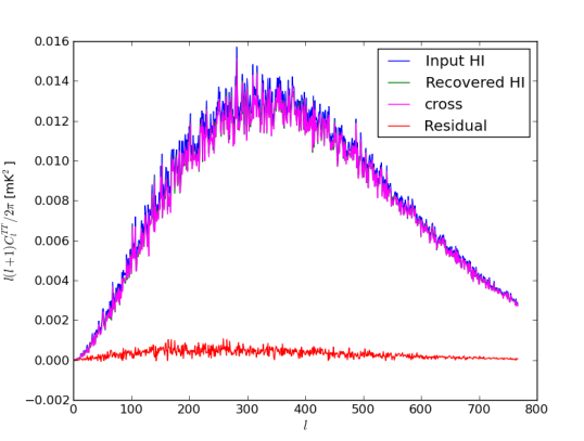
We can also check the recovery in spherical harmonic space, which is also what we are ultimately interested in cosmology. The cross angular power spectrum between the input and recovered map is defined as

$$C_{l}^{\text{cross}}=\frac{1}{2l+1}\sum_{m}\frac{1}{2}(a_{lm}^{\text{input}}a_{lm}^{\text{recover},*}+a_{lm}^{\text{input},*}a_{lm}^{\text{recover}}).$$

where $a_{lm}^{\text{input}},a_{lm}^{\text{recover}}$ are the spherical harmonic expansion coefficients for the input and recovered map respectively. The auto power spectrum for the input map, recovered map and the cross power are shown in Figure 5. These power spectra almost coincides with each other, and the residue difference is very small.

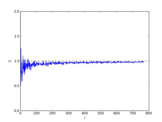
We can also compute the angular power transfer function $T_{l}=C_{l}^{\text{input}}/C_{l}^{\text{recovered}}$, which is shown as the bottom panel of Fig.5, which is nearly unity for the interested $\ell$ range, though the error is larger at small $l$ due to cosmic variance.

IV Comparison with the Classic PCA

In contrast to the classic PCA/SVD foreground subtraction method which only uses the low-rank structure and characteristics of the foregrounds implicitly, the RPCA method presented in this paper exploits the additional characteristics of the HI 21 cm signal frequency covariance matrix as well, which has a very sparse structure, as discussed in subsection II.1, only the elements along and near the main diagonal are non-zero. This improves the effectiveness of foreground subtraction, and is free from the 21 cm signal loss problem encountered in the classic PCA/SVD method.

To compare with the classic PCA method, we follow the method presented in Alonso et al. (2015); Bigot-Sazy et al. (2015). Diagonalize the frequency covariance matrix $\boldsymbol{\mathbf{R}}$ of the full data set with an eigen-decomposition,

$$\boldsymbol{\mathbf{U}}^{T}\boldsymbol{\mathbf{R}}\boldsymbol{\mathbf{U}}=\boldsymbol{\mathbf{\Lambda}}\equiv\text{diag}\{\lambda_{1},\cdots,\lambda_{N_{\nu}}\},$$ (31)

The magnitude of $\lambda_{i}$ gives the variance of the corresponding eigen-mode, each eigenvalue measures the contribution of its corresponding eigenvector to the total sky variance. As the foreground components dominate the full data overwhelmingly, we expect they would occupy the modes with the largest eigenvalues, so we pick a number of the largest eigenvalues $\lambda_{1}\geq\lambda_{2}\geq\cdots\lambda_{k}\geq 0$ to construct a matrix $\Lambda_{f}=\text{diag}\{\lambda_{1},\cdots,\lambda_{k},0,\cdots,0\}$, and use their corresponding eigenvectors to build a matrix $\boldsymbol{\mathbf{U}}_{f}$, then use this matrix to extract the foregrounds from the full data as $\hat{\boldsymbol{f}}=\boldsymbol{\mathbf{U}}_{f}\boldsymbol{\mathbf{U}}_{f}^{T}\boldsymbol{x}.$ Its covariance matrix is $\hat{\boldsymbol{\mathbf{R}}}_{f}=\frac{1}{N_{p}}\langle\hat{\boldsymbol{f}}\hat{\boldsymbol{f}}^{T}\rangle=\boldsymbol{\mathbf{U}}_{f}\boldsymbol{\mathbf{\Lambda}}_{f}\boldsymbol{\mathbf{U}}_{f}^{T},$ This is the solution of the classical PCA problem Eq. (17) with $M$ being the full data covariance matrix $\boldsymbol{\mathbf{R}}$ and $k$ being the number of largest eigenvalues corresponding to the contribution of foregrounds. The 21 cm signal can then be reconstructed by subtracting the foregrounds from the total data with $\hat{\boldsymbol{s}}=\boldsymbol{x}-\hat{\boldsymbol{f}}$.

Figure 6: Eigen-values of the covariance matrix $\boldsymbol{\mathbf{R}}$.

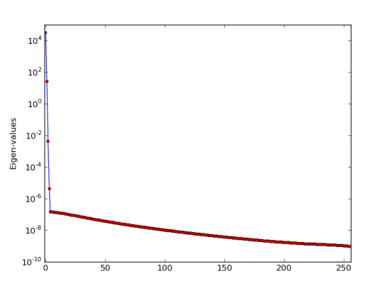
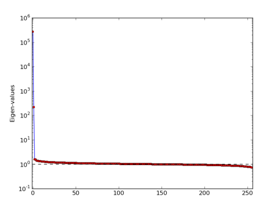
For our simulated data, we show the eigenvalues in Figure 6. We see that there are four eigenvalues which are significantly larger than others, the other eigenvalues decay slowly, which is different from that in Figure 3, where aside from the largest four eigenvalues, all others are quite close to 1, because by doing the transformation Equation 23, we have made the covariance matrix corresponding to the signal subspace close to identity. By subtracting the first 4 eigenmodes we obtain the reconstructed HI 21 cm signal.

Figure 7: Difference of RMSE (top) and Pearson correlation coefficient $r$ (bottom) between the RPCA+GILC method and the classical PCA method for all frequency points.

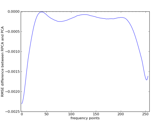
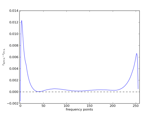
To compare the robust and classical PCA results, we introduce two quantitative aspects: the Root-Mean-Square Error (RMSE) and the Pearson correlation coefficient $r$. The former is defined as

$$\text{RMSE}=\sqrt{\sum\nolimits_{i}(x_{i}^{\text{input}}-x_{i}^{\text{recovered}})^{2}},$$

which reflects the total disagreement between the recovered 21 cm signal $\boldsymbol{x}^{\text{recovered}}$ and the input 21 cm signal $\boldsymbol{x}^{\text{input}}$; the latter is defined as

$$r=\frac{\sum_{i}(x_{i}^{\text{input}}-\bar{x}^{\text{input}})(x_{i}^{\text{recovered}}-\bar{x}^{\text{recovered}})}{\sqrt{\sum_{i}(x_{i}^{\text{input}}-\bar{x}^{\text{input}})^{2}}\sqrt{\sum_{i}(x_{i}^{\text{recovered}}-\bar{x}^{\text{recovered}})^{2}}},$$

which is a measure of the linear correlation between the recovered 21 cm signal $\boldsymbol{x}^{\text{recovered}}$ and the input 21 cm signal $\boldsymbol{x}^{\text{input}}$, where $\bar{x}^{\text{recovered}}$ and $\bar{x}^{\text{input}}$ are the mean of $\boldsymbol{x}^{\text{recovered}}$ and $\boldsymbol{x}^{\text{input}}$, respectively.

We show the difference of RMSE and $r$ between the two methods in Figure 7 for each frequency point, where we see the 21 cm signal recovered by the RPCA + GILC method is consistently better than that recovered by the classical PCA method in the whole frequency band, though in this case the difference is not large. This is probably because the foreground in our simulation can be well approximated by a rank-4 matrix, so the classical PCA extraction is already pretty good.

Figure 8: The line of sight temperature power spectrum $P_{21}(k_{\parallel})$ of the recovered 21 cm signal.

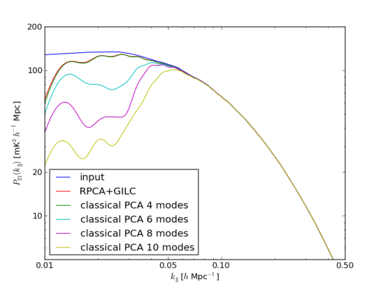
We plot the line of sight temperature power spectrum $P_{21}(k_{\parallel})$ of the recovered signal by the RPCA method and by the classical PCA method with different number of PCA modes being subtracted in Figure 8. Both performs well on small scales (large $k$). On the large scales (small $k$), the performance of both methods get worse as here the signal is more similar to the smooth foregrounds. The oscillating structure in the recovered $P_{21}(k_{\parallel})$ is due to the limited bandwidth (100 MHz) we have used. However, in the classical PCA the number of modes to be subtracted is more uncertain, as the decay of the eigenvalues is slower near the floor, as shown in Fig. 6, making it harder to decide how many modes should be subtracted. If the number of PCA modes being subtracted is incorrectly set (in this figure more than optimal 4 modes), the recovery performance of the classical PCA methods would become significantly worse as more modes with higher signal-to-foreground ratio are being subtracted, which causes the signal loss problem. For the recovery of the power spectrum, this signal-loss could be partially compensated by computing the signal loss transfer function from numerical simulations Masui et al. (2013); Switzer et al. (2013), but it is still a tricky and time-consuming process. In the RPCA method, at least in principle, the separation of the 21cm signal and the foreground is automatic, and as shown in Fig. 3 the eigenvalues are more distinctly separated.

However, despite the advantage of the RPCA method over the classic PCA method, in the recovered 21 cm signal and power spectrum the difference is not large. While we showed only one example above, we have tried various different realizations and different mean signal-to-foreground ratios, the results are generally similar to what we get here, the RPCA result is only slightly better than the best result of the classical PCA with optimal subtraction of modes. A possible reason for this is that the simulated foreground and beam models are so simple that the classical PCA already subtracted most of the foregrounds in the simulation. In practice, however, a much larger number of principal components must be subtracted from the the real observation data using the classical PCA. For example, in Ref. Masui et al. (2013), after many trials the first 20 modes are subtracted to get the 21 cm map. The signal loss would be quite severe, one needs to use simulation of mock samples to measure the power spectrum transfer function in the SVD in order to compensate for the signal loss. In that case the advantage of the RPCA method would be more significant. Analysis of the real data, however, require to deal with a number of practical issues. In the present paper we will concentrate on the algorithm itself, while the application to the observational data would be investigated in a subsequent study.

Figure 9: The relative recovery error of the 21 cm signal for the two method: red dots for the classical PCA method, green line for the RPCA method. $x$-axis is the number of modes subtracted by the classical PCA method.

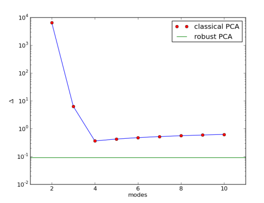
By utilizing both the low-rank property of the foreground frequency covariance and the sparsity of the 21 cm signal frequency covariance, the RPCA method can be used to subtract the foreground without losing the signal, which was encountered in the classic PCA method. However, the GILC reconstruction process may not be the best reconstruction method and also causes some signal loss too. To make a fair comparison of the RPCA with the classical PCA without being affected by the additional GILC part, we define a quantity $\Delta=\mathinner{\!\left\lVert\hat{\boldsymbol{\mathbf{R}}}_{\text{HI}}-\boldsymbol{\mathbf{R}}_{\text{HI}}\right\rVert}_{F}/\mathinner{\!\left\lVert\boldsymbol{\mathbf{R}}_{\text{HI}}\right\rVert}_{F}$ as the relative error between the recovered 21 cm signal frequency covariance matrix $\hat{\boldsymbol{\mathbf{R}}}_{\text{HI}}$ and the input 21 cm signal frequency covariance matrix $\boldsymbol{\mathbf{R}}_{\text{HI}}$. We show the relative error $\Delta$ in Figure 9 for the RPCA method and also the classical PCA method with different number of PCA modes subtracted, where $\hat{\boldsymbol{\mathbf{R}}}_{\text{HI}}$ is the sparse component $S$ for the RPCA method, and $\langle\hat{\boldsymbol{s}}\hat{\boldsymbol{s}}^{T}\rangle/N_{p}$ for the classical PCA method where $\hat{\boldsymbol{s}}$ is the recovered 21 cm signal. In Figure 9, we see a clear turning point at $N=4$ for the number of subtracted modes for the classical PCA method. This shows that the relative error decreases as we subtract the large PCA modes initially, but then the relative error begin to increase again as we subtract more modes, indicating more and more severe 21 cm signal loss during the classical PCA mode subtracting process. The relative recovery error of the RPCA method is about an order of magnitude lower than even the lowest relative error of the classical PCA method, indicating a better foreground subtraction and 21 cm signal recovery result.

We see that the RPCA method and the PCP algorithm are actually quite automatic in the sense that less tunable parameters are needed for the user to provide or tune, the regularization parameter $\lambda$ can be taken as $\sqrt{\max{(m,n)}}$ and works well in almost all cases, the user only need to provide an appropriate threshold $\delta$ for the iteration stopping criteria, Algorithm 1 automatically gets the matrices $L$ and $S$ satisfying the required low-rank and sparsity condition, the rank $k$ of $L$ and the number of non-zero elements and their support do not need to be known as a prior or to be determined, while for the classical PCA/SVD foreground subtraction, the user has to do several trials to determine the optimal number of principal components or SVD modes for a balance of good 21 cm signal recovery result and minimum signal loss.

V Discussion

We have shown by simulation that the RPCA method can efficiently extract the HI 21 cm $\nu-\nu^{\prime}$ covariance matrix from the observed data with better accuracy than the classical PCA method by utilizing the generic condition that the 21cm signal covariance matrix is sparse, while the foreground covariance matrix has low ranks. Algorithm 1 is very fast, only a relatively small number of iterations is needed to achieve good relative accuracy. For a $256\times 256$ matrix decomposition used in this simulation, it takes less than a minute on a personal computer to converge to a satisfactory error threshold. For higher pixel and frequency bin numbers, the speed of computation could be further accelerated by noting that instead of doing a full matrix SVD decomposition in each iteration, for calculating the singular value thresholding operator $\mathcal{D}_{\tau}(X)$ (step 3 in Algorithm 1), only those singular values that are greater than the threshold $\tau$ and the corresponding singular vectors are needed, so a partial SVD suffices Cai (2010). Some algorithms and softwares can do this, e.g., PROPACK and the modified version of LANSVD which comes with a threshold option to compute only those singular vectors with singular values greater than a given threshold value $\tau>0$.

In practice, artifacts are introduced in the sky maps reconstructed from the observatories during the map-making process, due to imperfections such as incomplete uv-coverage, missing data, particularly bright source, numerical errors. Usually the artifacts are not correlated with the HI 21 cm signal, though in some case may have correlations with the foregrounds, and may be distinct from both the foregrounds and the HI 21 cm signal. After removing some most obvious ones, residue artifacts should be small relative to the diffuse foregrounds and extragalactic point sources, though still larger than that of the HI 21 cm signal. Due to the complex structure and frequency dependence, its covariance matrix will not have a rank as low as that of the foregrounds, nor will it be sparse like that of the HI 21 cm signal. In the presence of artifacts, an extension of the RPCA method presented above is to include an additional term,

$$\boldsymbol{\mathbf{R}}=L+S+Z,$$

where $Z$ is a dense, small perturbation, which can be solved via the convex optimization problem called Stable Principle Component Pursuit (SPCP) Zhou et al. (2010):

$$\min_{L,S}\;\mathinner{\!\left\lVert L\right\rVert}_{*}+\lambda\mathinner{\!\left\lVert S\right\rVert}_{1}\quad\textup{s.t.}\quad\mathinner{\!\left\lVert\boldsymbol{\mathbf{R}}-L-S\right\rVert}_{F}\leq\delta.$$ (32)

Efficient algorithms for this problem are available Aybat et al. (2014); Aybat and Iyengar (2015).

The GILC method is used to recover the 21 cm signal from the observation data using the 21 cm $\nu-\nu^{\prime}$ covariance matrix extracted by the RPCA method. In this paper, the method is applied to the sky map as a whole, but in fact the foreground components may vary over different sky areas or different angular scales. Improvement can be made by employing the Generalized Needlet Internal Linear Combination (GNILC) method Remazeilles et al. (2011); Olivari et al. (2016), which worked in a needlet frame, the number of principal components of the observed covariance matrix is estimated locally both in space and in angular scale by using a wavelet (needlet) decomposition of the observations. We will explore how this extension could improve the recovery performance of the 21 cm signal in future work.

While we demonstrated the use of RPCA and GILC method for HI signal recovery in mid-redshift 21 cm experiment, it could also be applied to other redshift range (e.g. EoR) or even other spectral line (e.g. CO) intensity mapping experiments as well. For example, Olivari et al. (2016) showed that the GNILC method can be used to recover the 21 cm signal by using a prior of the theoretical HI frequency covariance matrix, here we have shown that actually we could extract a good estimate of the HI 21 cm frequency covariance matrix from the observed data itself by the RPCA method. This could avoid a biased prior, which is even more useful in the EoR 21cm experiment or other spectral line intensity mapping experiment, since in those cases we have less reliable knowledge of the expected signals.

Appendix A Generate the Simulated Maps

For the simulation of this paper, we use the software package CORA Shaw et al. (2014, 2015) to generate the input sky signals, including HI 21 cm signal and foreground components. For the HI emission, it assumes the Planck 2013 cosmological modelPlanck Collaboration et al. (2014). The foreground models used in CORA are based on Santos et al. (2005). However, for illustration purpose, here we only include two foreground components, the Galactic synchrotron emission and extragalactic point sources, which are the dominant components of the foreground contaminations related to 21 cm experiments and are also relatively accurately modeled ones. The angular power spectrum of these two components can both be modeled in the form of

$$C_{l}(\nu,\nu^{\prime})=A\left(\frac{l}{100}\right)^{-\alpha}\left(\frac{\nu\nu^{\prime}}{\nu_{0}^{2}}\right)^{-\beta}e^{-\frac{1}{2\xi_{l}^{2}}\ln^{2}(\nu/\nu^{\prime})}.$$ (33)

We use the recalibrated model parameters for the 700-800 MHz band of HI intensity mapping experiment. The CORA package also implemented the polarized emission model but for simplicity we only consider the total intensity model. The parameters of the models given in Equation 33 is listed in Table 2.

To generate the galactic synchrotron emission, CORA uses the processed 408 MHz Haslam map (bright point sources and striping are removed) as an template, and extrapolate to other frequencies using a spectral index from the Global Sky Model (GSM) Miville-Deschênes et al. (2008), with a Gaussian random realization of Equation 33 that adds fluctuations in frequency and on small angular scales. The extragalactic point sources simulations come from three components: a population of bright point sources ($S>10$ Jy at 151 MHz); a synthetic population of dimmer sources down to 0.1 Jy at 151 MHz; and an unresolved background of dimmer sources ($S<0.1$ Jy) modeled as a Gaussian random realization from Eq. (33) with the point source model parameters listed in Table 2.

On the scales of interest, the 21 cm power spectrum is given as

$$P_{T_{b}}(\boldsymbol{k};z,z^{\prime})=\bar{T}_{b}(z)\bar{T}_{b}(z^{\prime})(b+f\mu^{2})^{2}P_{m}(k;z,z^{\prime}),$$ (34)

where $b$ is the bias, $f$ is the growth rate, and $P_{m}(k;z,z^{\prime})$ is the real-space matter power spectrum. The mean brightness temperature, given in Chang et al. (2008), takes the form

$$\bar{T}_{b}(z) = 0.3\times\left(\frac{\Omega_{\text{HI}}}{10^{-3}}\right)\left(\frac{1+z}{2.5}\right)^{1/2}$$ (35)

$$\times\left(\frac{\Omega_{m}+(1+z)^{-3}\Omega_{\Lambda}}{0.29}\right)^{-1/2}\text{mK}.$$

We adopt the typical values of CORA parameters: $\Omega_{\text{HI}}b=6.2\times 10^{-3}$ Switzer et al. (2013) and $b=1$. The 21cm angular power spectrum is given by Datta et al. (2007)

$$C_{l}(\Delta\nu)\propto\int k^{2}dkj_{l}(kr_{\nu})j_{l}(kr_{\nu^{\prime}})P_{T_{b}}(\boldsymbol{k};z,z^{\prime}),$$

where $\Delta\nu=\nu^{\prime}-\nu$. CORA calculates a flat-sky approximation, which is accurate to the 1% level:

$$C_{l}(z,z^{\prime})=\frac{1}{\pi\chi\chi^{\prime}}\int_{0}^{\infty}dk_{\parallel}\cos(k_{\parallel}\Delta\chi)P_{T_{b}}(\boldsymbol{k};z,z^{\prime}),$$ (36)

where $\chi$ and $\chi^{\prime}$ are the comoving distances to redshift $z$ and $z^{\prime}$ and $\Delta\chi$ is their difference. See Refs. Shaw et al. (2014, 2015) and the CORA documentation for further details.

Table 2: Parameters for foreground model.

Component	Polarization	$A(\text{K}^{2})$	$\alpha$	$\beta$	$\xi$
Galaxy	TT	$6.6\times 10^{-3}$	2.80	2.8	4.0
Point sources	TT	$3.55\times 10^{-4}$	2.10	1.1	1.0

References

- Furlanetto et al. (2006) S. R. Furlanetto, S. P. Oh, and F. H. Briggs, Phys. Rep. 433, 181 (2006), astro-ph/0608032 .
- Morales and Wyithe (2010) M. F. Morales and J. S. B. Wyithe, ARA&A 48, 127 (2010), arXiv:0910.3010 .
- Pritchard and Loeb (2012) J. R. Pritchard and A. Loeb, Reports on Progress in Physics 75, 086901 (2012), arXiv:1109.6012 .
- Zaroubi (2013) S. Zaroubi, in The First Galaxies, Astrophysics and Space Science Library, Vol. 396, edited by T. Wiklind, B. Mobasher, and V. Bromm (2013) p. 45, arXiv:1206.0267 .
- Peterson et al. (2006) J. B. Peterson, K. Bandura, and U. L. Pen, ArXiv Astrophysics e-prints (2006), astro-ph/0606104 .
- Chang et al. (2008) T.-C. Chang, U.-L. Pen, J. B. Peterson, and P. McDonald, Physical Review Letters 100, 091303 (2008), arXiv:0709.3672 .
- Ansari et al. (2008) R. Ansari, J. . Le Goff, C. Magneville, M. Moniez, N. Palanque-Delabrouille, J. Rich, V. Ruhlmann-Kleider, and C. Yèche, ArXiv e-prints (2008), arXiv:0807.3614 .
- Seo et al. (2010) H.-J. Seo, S. Dodelson, J. Marriner, D. Mcginnis, A. Stebbins, C. Stoughton, and A. Vallinotto, ApJ 721, 164 (2010), arXiv:0910.5007 .
- Ansari et al. (2012) R. Ansari, J. E. Campagne, P. Colom, J. M. Le Goff, C. Magneville, J. M. Martin, M. Moniez, J. Rich, and C. Yèche, A&A 540, A129 (2012), arXiv:1108.1474 .
- Wang et al. (2006) X. Wang, M. Tegmark, M. G. Santos, and L. Knox, ApJ 650, 529 (2006), astro-ph/0501081 .
- Jelić et al. (2008) V. Jelić, S. Zaroubi, P. Labropoulos, R. M. Thomas, G. Bernardi, M. A. Brentjens, A. G. de Bruyn, B. Ciardi, G. Harker, L. V. E. Koopmans, V. N. Pandey, J. Schaye, and S. Yatawatta, MNRAS 389, 1319 (2008), arXiv:0804.1130 .
- Liu et al. (2009a) A. Liu, M. Tegmark, and M. Zaldarriaga, MNRAS 394, 1575 (2009a), arXiv:0807.3952 .
- Liu et al. (2009b) A. Liu, M. Tegmark, J. Bowman, J. Hewitt, and M. Zaldarriaga, MNRAS 398, 401 (2009b), arXiv:0903.4890 [astro-ph.CO] .
- Masui et al. (2013) K. W. Masui, E. R. Switzer, N. Banavar, K. Bandura, C. Blake, L.-M. Calin, T.-C. Chang, X. Chen, Y.-C. Li, Y.-W. Liao, A. Natarajan, U.-L. Pen, J. B. Peterson, J. R. Shaw, and T. C. Voytek, ApJ 763, L20 (2013), arXiv:1208.0331 [astro-ph.CO] .
- Bigot-Sazy et al. (2015) M.-A. Bigot-Sazy, C. Dickinson, R. A. Battye, I. W. A. Browne, Y.-Z. Ma, B. Maffei, F. Noviello, M. Remazeilles, and P. N. Wilkinson, MNRAS 454, 3240 (2015), arXiv:1507.04561 .
- Switzer et al. (2013) E. R. Switzer, K. W. Masui, K. Bandura, L.-M. Calin, T.-C. Chang, X.-L. Chen, Y.-C. Li, Y.-W. Liao, A. Natarajan, U.-L. Pen, J. B. Peterson, J. R. Shaw, and T. C. Voytek, MNRAS 434, L46 (2013), arXiv:1304.3712 [astro-ph.CO] .
- Switzer et al. (2015) E. R. Switzer, T.-C. Chang, K. W. Masui, U.-L. Pen, and T. C. Voytek, ApJ 815, 51 (2015), arXiv:1504.07527 .
- Chapman et al. (2012) E. Chapman, F. B. Abdalla, G. Harker, V. Jelić, P. Labropoulos, S. Zaroubi, M. A. Brentjens, A. G. de Bruyn, and L. V. E. Koopmans, MNRAS 423, 2518 (2012), arXiv:1201.2190 [astro-ph.CO] .
- Wolz et al. (2014) L. Wolz, F. B. Abdalla, C. Blake, J. R. Shaw, E. Chapman, and S. Rawlings, MNRAS 441, 3271 (2014), arXiv:1310.8144 .
- Alonso et al. (2015) D. Alonso, P. Bull, P. G. Ferreira, and M. G. Santos, MNRAS 447, 400 (2015), arXiv:1409.8667 .
- Chapman et al. (2013) E. Chapman, F. B. Abdalla, J. Bobin, J.-L. Starck, G. Harker, V. Jelić, P. Labropoulos, S. Zaroubi, M. A. Brentjens, A. G. de Bruyn, and L. V. E. Koopmans, MNRAS 429, 165 (2013), arXiv:1209.4769 [astro-ph.CO] .
- Candès et al. (2006) E. J. Candès, J. Romberg, and T. Tao, IEEE Transactions on information theory 52, 489 (2006).
- Donoho (2006) D. L. Donoho, IEEE Trans. Inform. Theory 52, 1289 (2006).
- Rockafellar (1970) R. Rockafellar, Convex Analysis, Princeton landmarks in mathematics and physics (Princeton University Press, 1970).
- Boyd and Vandenberghe (2004) S. Boyd and L. Vandenberghe, Convex Optimization (Cambridge University Press, New York, NY, USA, 2004).
- Bobin et al. (2008) J. Bobin, J.-L. Starck, and R. Ottensamer, IEEE Journal of Selected Topics in Signal Processing 2, 718 (2008), arXiv:0802.0131 .
- Carrillo et al. (2013) R. E. Carrillo, J. D. McEwen, D. Van De Ville, J.-P. Thiran, and Y. Wiaux, IEEE Signal Processing Letters 20, 591 (2013), arXiv:1208.2330 [cs.IT] .
- Carrillo et al. (2014) R. E. Carrillo, J. D. McEwen, and Y. Wiaux, MNRAS 439, 3591 (2014), arXiv:1307.4370 [astro-ph.IM] .
- Carrillo et al. (2015) R. Carrillo, V. Kartik, J.-P. Thiran, and Y. Wiaux, in Signal Processing with Adaptive Sparse Structured Representations Workshop (2015).
- Garsden et al. (2015) H. Garsden, J. N. Girard, J. L. Starck, S. Corbel, C. Tasse, A. Woiselle, J. P. McKean, A. S. van Amesfoort, J. Anderson, I. M. Avruch, R. Beck, M. J. Bentum, P. Best, F. Breitling, J. Broderick, M. Brüggen, H. R. Butcher, B. Ciardi, F. de Gasperin, E. de Geus, M. de Vos, S. Duscha, J. Eislöffel, D. Engels, H. Falcke, R. A. Fallows, R. Fender, C. Ferrari, W. Frieswijk, M. A. Garrett, J. Grießmeier, A. W. Gunst, T. E. Hassall, G. Heald, M. Hoeft, J. Hörandel, A. van der Horst, E. Juette, A. Karastergiou, V. I. Kondratiev, M. Kramer, M. Kuniyoshi, G. Kuper, G. Mann, S. Markoff, R. McFadden, D. McKay-Bukowski, D. D. Mulcahy, H. Munk, M. J. Norden, E. Orru, H. Paas, M. Pandey-Pommier, V. N. Pandey, G. Pietka, R. Pizzo, A. G. Polatidis, A. Renting, H. Röttgering, A. Rowlinson, D. Schwarz, J. Sluman, O. Smirnov, B. W. Stappers, M. Steinmetz, A. Stewart, J. Swinbank, M. Tagger, Y. Tang, C. Tasse, S. Thoudam, C. Toribio, R. Vermeulen, C. Vocks, R. J. van Weeren, S. J. Wijnholds, M. W. Wise, O. Wucknitz, S. Yatawatta, P. Zarka, and A. Zensus, A&A 575, A90 (2015), arXiv:1406.7242 [astro-ph.IM] .
- Girard et al. (2015) J. N. Girard, H. Garsden, J. L. Starck, S. Corbel, A. Woiselle, C. Tasse, J. P. McKean, and J. Bobin, Journal of Instrumentation 10, C08013 (2015), arXiv:1504.03896 [astro-ph.IM] .
- Ferrari et al. (2015) A. Ferrari, J. Deguignet, C. Ferrari, D. Mary, A. Schutz, and O. Smirnov, ArXiv e-prints (2015), arXiv:1504.06847 [astro-ph.IM] .
- Onose et al. (2016a) A. Onose, R. E. Carrillo, A. Repetti, J. D. McEwen, J.-P. Thiran, J.-C. Pesquet, and Y. Wiaux, MNRAS 462, 4314 (2016a), arXiv:1601.04026 [astro-ph.IM] .
- Onose et al. (2016b) A. Onose, R. E. Carrillo, J. D. McEwen, and Y. Wiaux, ArXiv e-prints (2016b), arXiv:1610.08895 [astro-ph.IM] .
- Högbom (1974) J. A. Högbom, A&AS 15, 417 (1974).
- Wakker and Schwarz (1988) B. P. Wakker and U. J. Schwarz, A&A 200, 312 (1988).
- Lannes et al. (1997) A. Lannes, E. Anterrieu, and P. Marechal, A&AS 123 (1997), 10.1051/aas:1997312.
- Bharadwaj and Ali (2005) S. Bharadwaj and S. S. Ali, MNRAS 356, 1519 (2005), astro-ph/0406676 .
- Datta et al. (2007) K. K. Datta, T. R. Choudhury, and S. Bharadwaj, MNRAS 378, 119 (2007), astro-ph/0605546 .
- Candès et al. (2011) E. J. Candès, X. Li, Y. Ma, and J. Wright, J. ACM 58, 11:1 (2011).
- Wright et al. (2009) J. Wright, A. Ganesh, S. Rao, Y. Peng, and Y. Ma, in Advances in Neural Information Processing Systems 22, edited by Y. Bengio, D. Schuurmans, J. D. Lafferty, C. K. I. Williams, and A. Culotta (Curran Associates, Inc., 2009) pp. 2080–2088.
- Chandrasekaran et al. (2011) V. Chandrasekaran, S. Sanghavi, P. A. Parrilo, and A. S. Willsky, SIAM Journal on Optimization 21, 572 (2011).
- Natarajan (1995) B. K. Natarajan, SIAM J. Comput. 24, 227 (1995).
- Recht et al. (2010) B. Recht, M. Fazel, and P. A. Parrilo, SIAM Rev. 52, 471 (2010).
- Candès and Recht (2008) E. J. Candès and B. Recht, CoRR abs/0805.4471 (2008).
- Hornstein (2011) M. Hornstein, Rose-Hulman Undergraduate Mathematics Journal 12 (2011).
- Liu and Vandenberghe (2009) Z. Liu and L. Vandenberghe, SIAM J. Matrix Analysis Applications 31, 1235 (2009).
- Mohan and Fazel (2012) K. Mohan and M. Fazel, J. Mach. Learn. Res. 13, 3441 (2012).
- Boyd et al. (2003) S. P. Boyd, L. Xiao, and A. Mutapcic, in stanford.edu (2003).
- Lin et al. (2009) Z. Lin, A. Ganesh, J. Wright, L. Wu, M. Chen, and Y. Ma, in In Intl. Workshop on Comp. Adv. in Multi-Sensor Adapt. Processing, Aruba, Dutch Antilles (2009).
- Eckstein and Yao (2012) J. Eckstein and W. Yao, RUTCOR Research Reports 32 (2012).
- Boyd et al. (2011) S. Boyd, N. Parikh, E. Chu, B. Peleato, and J. Eckstein, Found. Trends Mach. Learn. 3, 1 (2011).
- Lin et al. (2010) Z. Lin, M. Chen, and Y. Ma, ArXiv e-prints (2010), arXiv:1009.5055 [math.OC] .
- Netrapalli et al. (2014) P. Netrapalli, N. U N, S. Sanghavi, A. Anandkumar, and P. Jain, in Advances in Neural Information Processing Systems 27, edited by Z. Ghahramani, M. Welling, C. Cortes, N. D. Lawrence, and K. Q. Weinberger (Curran Associates, Inc., 2014) pp. 1107–1115.
- Kang et al. (2015) Z. Kang, C. Peng, and Q. Cheng, in 2015 IEEE International Conference on Data Mining (2015) pp. 211–220.
- Yi et al. (2016) X. Yi, D. Park, Y. Chen, and C. Caramanis, CoRR abs/1605.07784 (2016), arXiv:1605.07784 .
- Yuan and Yang (2009) X. Yuan and J. Yang, optimization-online.org (2009).
- Cai et al. (2010) J.-F. Cai, E. J. Candès, and Z. Shen, SIAM J. on Optimization 20, 1956 (2010).
- Shaw et al. (2014) J. R. Shaw, K. Sigurdson, U.-L. Pen, A. Stebbins, and M. Sitwell, ApJ 781, 57 (2014), arXiv:1302.0327 [astro-ph.CO] .
- Shaw et al. (2015) J. R. Shaw, K. Sigurdson, M. Sitwell, A. Stebbins, and U.-L. Pen, Phys. Rev. D 91, 083514 (2015), arXiv:1401.2095 .
- Chen (2012) X. Chen, International Journal of Modern Physics Conference Series 12, 256 (2012), arXiv:1212.6278 [astro-ph.IM] .
- Górski et al. (2005) K. M. Górski, E. Hivon, A. J. Banday, B. D. Wandelt, F. K. Hansen, M. Reinecke, and M. Bartelmann, ApJ 622, 759 (2005), astro-ph/0409513 .
- Chang et al. (2010) T.-C. Chang, U.-L. Pen, K. Bandura, and J. B. Peterson, Nature 466, 463 (2010).
- Remazeilles et al. (2011) M. Remazeilles, J. Delabrouille, and J.-F. Cardoso, MNRAS 418, 467 (2011), arXiv:1103.1166 .
- Bennett et al. (2003) C. L. Bennett, R. S. Hill, G. Hinshaw, M. R. Nolta, N. Odegard, L. Page, D. N. Spergel, J. L. Weiland, E. L. Wright, M. Halpern, N. Jarosik, A. Kogut, M. Limon, S. S. Meyer, G. S. Tucker, and E. Wollack, ApJS 148, 97 (2003), astro-ph/0302208 .
- Tegmark et al. (2003) M. Tegmark, A. de Oliveira-Costa, and A. J. Hamilton, Phys. Rev. D 68, 123523 (2003), astro-ph/0302496 .
- Delabrouille et al. (2009) J. Delabrouille, J.-F. Cardoso, M. Le Jeune, M. Betoule, G. Fay, and F. Guilloux, A&A 493, 835 (2009), arXiv:0807.0773 .
- Olivari et al. (2016) L. C. Olivari, M. Remazeilles, and C. Dickinson, MNRAS 456, 2749 (2016), arXiv:1509.00742 .
- Cai (2010) J. F. Cai, UCLA CAM Report (2010).
- Zhou et al. (2010) Z. Zhou, X. Li, J. Wright, E. C, and Y. Ma, in in International Symposium on Information Theory (2010).
- Aybat et al. (2014) N. S. Aybat, D. Goldfarb, and S. Ma, Computational Optimization and Applications 58, 1 (2014).
- Aybat and Iyengar (2015) N. S. Aybat and G. Iyengar, Comput. Optim. Appl. 61, 635 (2015).
- Planck Collaboration et al. (2014) Planck Collaboration, P. A. R. Ade, N. Aghanim, C. Armitage-Caplan, M. Arnaud, M. Ashdown, F. Atrio-Barandela, J. Aumont, C. Baccigalupi, A. J. Banday, and et al., A&A 571, A16 (2014), arXiv:1303.5076 .
- Santos et al. (2005) M. G. Santos, A. Cooray, and L. Knox, ApJ 625, 575 (2005), astro-ph/0408515 .
- Miville-Deschênes et al. (2008) M.-A. Miville-Deschênes, N. Ysard, A. Lavabre, N. Ponthieu, J. F. Macías-Pérez, J. Aumont, and J. P. Bernard, A&A 490, 1093 (2008), arXiv:0802.3345 .