Singlet fermionic dark matter with Veltman conditions

Abstract

We reexamine a renormalizable model of a fermionic dark matter with a gauge singlet Dirac fermion and a real singlet scalar which can ameliorate the scalar mass hierarchy problem of the Standard Model (SM). Our model setup is the minimal extension of the SM for which a realistic dark matter (DM) candidate is provided and the cancellation of one-loop quadratic divergence to the scalar masses can be achieved by the Veltman condition (VC) simultaneously. This model extension, although renormalizable, can be considered as an effective low-energy theory valid up to cut-off energies about 10 TeV. We calculate the one-loop quadratic divergence contributions of the new scalar and fermionic DM singlets, and constrain the model parameters using the VC and the perturbative unitarity conditions. Taking into account the invisible Higgs decay measurement, we show the allowed region of new physics parameters satisfying the recent measurement of relic abundance. With the obtained parameter set, we predict the elastic scattering cross section of the new singlet fermion into target nuclei for a direct detection of the dark matter. We also perform the full analysis with arbitrary set of parameters without the VC as a comparison, and discuss the implication of the constraints by the VC in detail.

I Introduction

Recent discovery of a Higgs-like boson at the LHC ATLAS12 ; CMS12 completes the standard model (SM) as a renormalizable theory, and its observed mass $M_{h}=125.9\pm 0.4$ GeV validates the perturbativity of weak interactions in the model Lee77 . In the SM, a scalar mass receives additive quantum corrections proportional to the momentum cut-off squared, $\Lambda^{2}$ at one-loop level. This quadratically divergent one-loop correction to the Higgs mass was first calculated by Veltman Veltman81 , and given by

$$\delta M_{h}^{2}=\frac{3\Lambda^{2}}{16\pi^{2}v_{h}^{2}}\left(M_{h}^{2}+2M_{W}^{2}+M_{Z}^{2}-4m_{t}^{2}\right),$$ (1)

where $v_{h}$ is the vacuum expectation value (VEV) of the Higgs field and only the dominant contribution is shown in the scale $\Lambda$. If $\Lambda$ is very large, the Higgs mass suffers from the quadratic divergence of this correction, which addresses the naturalness issue of the theory resulting in the fine-tuning problem Susskind79 . Since the cut-off scale $\Lambda$ is considered to be UV boundary of the SM Georgi74 , it would be more natural that the cancellation of the quadratic divergences could be achieved by means of a symmetry principle at higher scales rather than by fine-tuning of mathematically supplemented counterterms. There have been various extensions of the SM to resolve the fine-tuning (or the hierarchy) problem of the Higgs mass by canceling the quadratic divergences such as the supersymmetry (SUSY) and the little Higgs model (LHM). However no compelling sign of evidence for new physics (NP) beyond the SM has been found at the LHC.

Veltman has suggested the cancellation of the quadratic divergence of the Eq. (1) by itself leading to the prediction of the Higgs mass, which is called the Veltman condition (VC). It might imply the existence of some hidden symmetry though the underlying theory is unknown. The simple VC predicted $M_{h}\sim 320$ GeV with the known particle masses at present ,and does not hold in the SM with the present measured value $M_{h}\sim 125$ GeV. In order to impose the VC to the Higgs mass, required are some new degrees of freedom which interact with the Higgs boson to contribute to the Higgs self-energy diagram Gunion08 . Simple extensions of the SM resolving the fine-tuning problem by applying the VC have been studied widely in many literatures Grzadkowski09 ; Pivovarov08 ; Masina13 ; Karahan14 ; Demir15 .

Besides the fine-tuning issue, there are other motivations to search for the NP beyond the SM. One of the most important motivation is the existence of the distinct observational evidence for dark matter (DM). Thus many viable DM candidates have been suggested in various NP models at present. In order to include DM in the SM framework, we should assume the existence of additional degrees of freedom. Since any SM particle cannot be DM, DM itself should be a new degree of freedom, and new particles or new interactions are also required to connect the DM and the SM sector. In the Higgs portal model for the DM, only the Higgs quadratic term takes part in interacting with the new degrees of freedom. Thus the Higgs portal model can provide both of the DM and the interaction of new degrees of freedom with the Higgs boson to satisfy the VC for the Higgs mass. Recently there has been some efforts to investigate a possibility to explain the fine-tuning of the Higgs mass through the VC in the Higgs portal model for the dark matter. One of the simplest extension to satisfy the VC is to introduce only one new scalar to cancel the dominant top contribution in Eq. (1) Karahan14 ; Demir15 . New scalar degrees of freedom for ameliorating the fine-tuning problem could be DM candidates in itself interacting with the SM sector through Higgs portal with a discrete $Z_{2}$ symmetry Drozd12 . However, a new quadratic divergence to the new scalar DM mass arises in this minimal model and we have to resolve it as well. For instance, we may introduce additional vector-like fermions to cancel the new quadratic divergence and to protect the masses of the Higgs boson and the new scalar DM simultaneously Chakraborty13 .

Alternatively we consider the Higgs portal model with the singlet fermionic dark matter as a more general scenario in this paper since this model was first introduced by our earlier studies Lee07 . In this model, we have a Dirac fermion and a real scalar, which are both the SM gauge singlets. If we assign no $Z_{2}$ symmetry, the singlet scalar cannot be a DM since it would decay into the SM sector through mixing. Thus the DM is the singlet fermion in this model. We impose the VC on the quadratic divergences of both scalar masses of the SM-like Higgs boson and the singlet scalar in our model. Under the VC, we still find the allowed parameter space where the singlet fermion satisfies the observed relic density constraints to be the DM candidates. It implies that our model of the DM provides the improved naturalness at least at one-loop level. Since the VC is a very strong condition to fix the Higgs-scalar coupling $\lambda_{2}$ to a specific value, only the limited parameter sets are allowed. Also explored is the direct detections of the singlet fermion through the DM-nucleon scattering under the VC and the prospect of observation of the DM in the future is discussed in this paper. All the analyses are performed with the up-to-date cosmological data without applying the VC as well in order to clearly see the implication of the VC constraints and also for the general DM study as a reference. This model might provide richer phenomenology especially in the studies of the electroweak phase transition responsible for the baryon asymmetry in the early universe PMS .

This paper is organized as follows. In Sec. II, we briefly review our model and summarize the model parameters. We discuss the VCs for the scalar masses in Sec. III and constraints from the measurements of Higgs decays in Sec. IV. Studied are phenomenologies for the dark matter such as the relic density and the direct detection through DM-nucleon scattering in Sec. V. Finally we conclude in Sec. VI.

II model

We adopt a dark sector consisting of a real scalar field $S$ and a Dirac fermion field $\psi$ which are SM gauge singlets studied first in Ref. Lee07 ; Kim16 . The dark sector Lagrangian with the renormalizable interactions is then given by

$$\mathcal{L}_{DM}=\bar{\psi}\left(i\partial\!\!\!/-M_{\psi_{0}}\right)\psi+\frac{1}{2}\left(\partial_{\mu}S\right)\left(\partial^{\mu}S\right)-g_{S}\bar{\psi}\psi S-V_{S}(S,H),$$ (2)

where the Higgs portal potential is

$$V_{S}(S,H)=\frac{1}{2}M_{S}^{2}S^{2}+\lambda_{1}H^{\dagger}HS+\lambda_{2}H^{\dagger}HS^{2}+\frac{\lambda_{3}}{3!}S^{3}+\frac{\lambda_{4}}{4!}S^{4}.$$ (3)

Note that the singlet fermionic DM field $\psi$ couples only to the singlet scalar $S$, and the interactions of the singlet sector to the SM sector arise only through the Higgs portal $H^{\dagger}H$. After electroweak symmetry breaking, the neutral component of the SM Higgs and the singlet scalar develop nonzero VEVs, $\langle H^{0}\rangle=v_{h}/\sqrt{2}$ and $\langle S\rangle=v_{s}$, respectively.

Minimizing the full scalar potentials $V_{S}+V_{SM}$, where

$$V_{SM}=-\mu^{2}H^{\dagger}H+\lambda_{0}(H^{\dagger}H)^{2},$$ (4)

the scalar mass parameters $M_{S}^{2}$ and $\mu^{2}$ are expressed in terms of the scalar VEVs as follows PMS

$$M_{S}^{2} = -\left(\frac{\lambda_{1}}{2v_{s}}+\lambda_{2}\right)v_{h}^{2}-\left(\frac{\lambda_{3}}{2v_{s}}+\frac{\lambda_{4}}{6}\right)v_{s}^{2},$$

$$\mu^{2} = {\lambda}_{0}v_{h}^{2}+(\lambda_{1}+\lambda_{2}v_{s})v_{s}.$$ (5)

The neutral scalar fields $h$ and $s$ defined by $H^{0}=(v_{h}+h)/\sqrt{2}$ and $S=v_{s}+s$ are mixed to yield the mass matrix given by

$$\mu_{h}^{2} = 2{\lambda}_{0}v_{h}^{2},$$

$$\mu_{s}^{2} = -\frac{\lambda_{1}v_{h}^{2}}{2v_{s}}+\frac{\lambda_{3}}{2}v_{s}+\frac{\lambda_{4}}{3}v_{s}^{2},$$

$$\mu_{hs}^{2} = (\lambda_{1}+2\lambda_{2}v_{s})v_{h}.$$ (6)

The corresponding scalar mass eigenstates $h_{1}$ and $h_{2}$ are admixtures of $h$ and $s$,

$$\left(\begin{array}[]{c}h_{1}\\[1.0pt] h_{2}\end{array}\right)=\left(\begin{array}[]{cc}\cos\theta&\ \sin\theta\\[1.0pt] -\sin\theta&\ \cos\theta\end{array}\right)\left(\begin{array}[]{c}h\\[1.0pt] s\end{array}\right),$$ (7)

where the mixing angle $\theta$ is given by

$$\tan\theta=\frac{y}{1+\sqrt{1+y^{2}}},$$ (8)

with $\ y\equiv 2\mu_{hs}^{2}/(\mu_{h}^{2}-\mu_{s}^{2})$. After the mass matrix is diagonalized, we obtain the physical masses of the two scalar bosons $h_{1,2}$ as follows:

$$M^{2}_{1,2}=\frac{\mu_{h}^{2}+\mu_{s}^{2}}{2}\pm\frac{\mu_{h}^{2}-\mu_{s}^{2}}{2}\sqrt{1+y^{2}},$$ (9)

where the upper (lower) sign corresponds to $M_{1}(M_{2})$. We assume that $M_{1}$ corresponds to the observed SM-like Higgs boson mass in what follows.

The singlet fermion $\psi$ has mass $M_{\psi}=M_{\psi_{0}}+g_{S}v_{s}$ as an independent parameter of the model since $M_{\psi_{0}}$ is just a free model parameter, and the Yukawa coupling $g_{S}$ measures the interaction of $\psi$ with singlet component of the scalar particles. In total, we have eight independent model parameters relevant for DM phenomenology. The six model parameters $\lambda_{0},\lambda_{1},\lambda_{2},\lambda_{3},\lambda_{4}$ and $v_{s}$ determine the masses $M_{1,2}$, the mixing angle $\theta$, and self-couplings of the two physical scalars $h_{1,2}$. Given the fixed Higgs mass $M_{1}$, we constrain seven independent NP parameters taking into account various theoretical consideration and experimental measurements in the next section.

III Veltman condition and Unitarity

(a)

(b)

Figure 1: One-loop quadratic divergence contributions of the (a) scalars and (b) fermionic DM to the Higgs and the new scalar masses from the hidden sector.

We apply the VC to this model as done similarly in Refs.Chakraborty13 ; Karahan14 ; Demir15 , and constrain the above model parameters from the fine-tuning problem originating from the radiative corrections to the Higgs mass. Cutting off the loop integral momenta at a scale $\Lambda$, and keeping only the dominant contributions in this scale, we obtain

$$M^{2}_{h}=(M^{0}_{h})^{2}+\frac{3\Lambda^{2}}{16\pi^{2}v_{h}^{2}}\left(M_{h}^{2}+2M_{W}^{2}+M_{Z}^{2}-4m_{t}^{2}+\frac{\lambda_{2}}{3}v_{h}^{2}\right),$$ (10)

where $M^{0}_{h}$ is the bare mass constrained in the unrenormalized Lagrangian, and small mixing effect proportional to $\theta$ is neglected. The last term proportional to $\lambda_{2}$ in Eq. (10) is obtained from the one-loop diagram in Fig. 1(a). Following Veltman Veltman81 , note that by choosing the parameter $\lambda_{2}$ to be

$$\lambda_{2}=3(4m_{t}^{2}-M_{h}^{2}-2M_{W}^{2}-M_{Z}^{2})/v_{h}^{2}\sim 4.17,$$ (11)

the quadratic divergences can be canceled and this could be a prediction for the parameter $\lambda_{2}$. This result agrees well with the prior result of Ref. Demir15 where the additional scalar mass is protected by a new hidden vector. Also, the same result for $\lambda_{2}$ was obtained in the (multi-)scalar DM model studied in Ref. Chakraborty13 . On the other hand, in our model, a singlet fermionic DM stabilizes the mass of the scalar mediator. Similarly to the Higgs mass case, as for the scalar singlet mass, we obtain from Fig. 1 that

$$M^{2}_{s}=(M^{0}_{s})^{2}+\frac{\Lambda^{2}}{32\pi^{2}}\left(\lambda_{4}+2\lambda_{2}-8g_{S}^{2}\right),$$ (12)

and the VC requires

$$\lambda_{4}=8g_{S}^{2}-2\lambda_{2}.$$ (13)

The conditions obtained above were given only at the one-loop level, and cannot be the legitimate solution to the fine-tuning problem especially if the scale of NP is extremely large. For scales not much larger than the electroweak scale, however, one does not need very large cancellations. If the Veltman solution is by chance satisfied, the scale $\Lambda$ can be pushed at the two-loop level to a much higher value proportional to $\Lambda^{2}\log\Lambda$ for $\Lambda\sim 15$ TeV. Nonetheless, including two-loop (or higher-loop) corrections will modify the above condition by further powers of $O(1/16\pi^{2})$, so that a modification of the one-loop VC is very small at the level of a few percent Al-sarhi92 . Of course, one can set up the model parameters to apply the VC at the two-loop or higher level.

The couplings $\lambda_{2,4}$ can grow significantly with increasing renormalization scale $\Lambda$, and one can constraint those by applying the tree-level perturbative unitarity to scalar elastic scattering processes for the zeroth partial wave amplitude Lee77 . For a singlet scalar Higgs portal, the bounds on the couplings $\lambda_{2,4}$ are given by Cynolter04

$$|\lambda_{2}|\leq 4\pi,\quad\lambda_{4}\leq 8\pi.$$ (14)

The value of $\lambda_{2}$ obtained from the VC in Eq.(11) lies obviously in the range of the above bound. From the fact that the quartic coupling $\lambda_{4}$ should be positive, and from Eqs. (13) and (14) we obtain

$$1.02<g_{S}<2.05.$$ (15)

Interestingly, the obtained size of allowed DM coupling $g_{S}$ is similar to that of the strong interaction coupling in the SM. Using the given conditions, we will perform the numerical analysis with the various sets of the following five NP parameters: $\sin\theta,M_{2},M_{\psi},g_{S},v_{s}$. In addition, we will also show the full analysis with arbitrary set of $\lambda_{2,4}$ without the VC as a comparison.

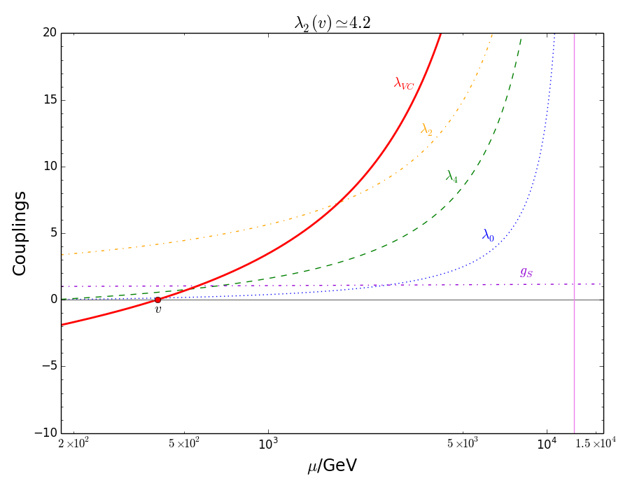
(a)

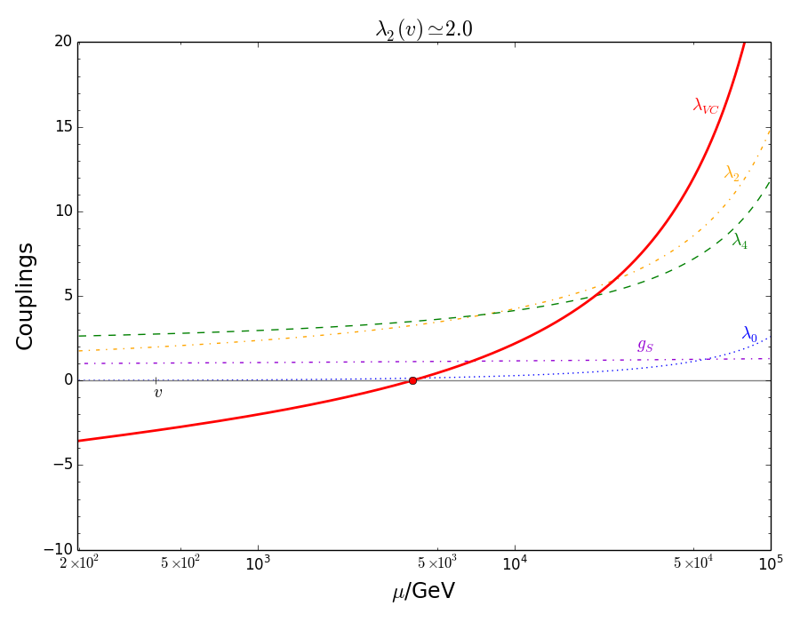
(b)

Figure 2: Running of the massless couplings and the first VC given in Eq. (17) for (a) $\lambda_{2}(v)=4.17$ and (b) $\lambda_{2}(v)=2.0$ with the renormalization scale $\mu$. The vertical(violet) line indicates where one of the couplings hits Landau pole. $g_{S}$ and $\lambda_{4}$ are chosen to satisfy the second VC obtained in Eq. (13) at (a) $\mu=v$ and (b) $\mu=4$ TeV.

Before we discuss the phenomenological aspects of this model in the next section, we briefly check the renormalization group evolution (RGE) behavior of the model parameters. The $\beta$-function of a coupling $\lambda_{i}$ at a scale $\mu$ in the RGE is defined as $\beta_{\lambda_{i}}=\partial\lambda_{i}/\partial\log\mu$. For dimensionless couplings in the scalar potential (including the DM Yukawa coupling), the one-loop $\beta$-functions are given by Baek12

$$\beta_{\lambda_{0}}^{(1)} = \frac{1}{16\pi^{2}}\left[24\lambda_{0}^{2}+12\lambda_{0}\lambda_{t}^{2}-6\lambda_{t}^{4}-3\lambda_{0}(3g_{2}^{2}+g_{1}^{2})+\frac{3}{8}\big{(}2g_{2}^{4}+(g_{2}^{2}+g_{1}^{2})^{2}\big{)}+2\lambda_{2}^{2}\right],$$

$$\beta_{\lambda_{2}}^{(1)} = \frac{\lambda_{2}}{16\pi^{2}}\left[12\lambda_{0}-\frac{3}{2}\lambda_{0}(3g_{2}^{2}+g_{1}^{2})+6\lambda_{t}^{2}+8\lambda_{2}+\lambda_{4}+4g_{S}^{2}\right],$$

$$\beta_{\lambda_{4}}^{(1)} = \frac{1}{16\pi^{2}}\left[8\lambda_{2}^{2}+\frac{1}{2}\lambda_{4}^{2}+\frac{4}{3}\lambda_{4}g_{S}^{2}-8g_{S}^{4}\right],\qquad\beta_{g_{S}}^{(1)}=\frac{5}{16\pi^{2}}g_{S}^{3},$$ (16)

where $g_{1}$ and $g_{2}$ are the SM U$(1)_{Y}$ and SU$(2)_{L}$ couplings, respectively, and $\lambda_{t}$ is the top Yukawa coupling. In terms of the running couplings, the quadratic radiative mass correction $\delta M_{h}^{2}$ in Eq. (11) can be rewritten at a scale $\mu$ as

$$\delta M_{h}^{2}(\mu)\equiv\frac{\Lambda^{2}}{16\pi^{2}}\lambda_{VC}(\mu)=\frac{\Lambda^{2}}{16\pi^{2}}\left(6\lambda_{0}(\mu)+\frac{9}{4}g_{2}^{2}(\mu)+\frac{3}{4}g_{1}^{2}(\mu)-6\lambda_{t}^{2}(\mu)+\lambda_{2}(\mu)\right).$$ (17)

It is natural to determine the values of the physical observables at a scale $\mu=v\equiv\sqrt{v_{h}^{2}+v_{s}^{2}}$ for a study of the DM phenomenology since $v$ can be considered as the VEV of the radial component of a scalar field composed of $h$ and $s$. Since we are interested in the DM fermion (and $h_{2}$) lighter than 1 TeV, we choose $v\sim 400$ GeV as a benchmark point. In Fig. 2, we show the scale dependence on the RGE of the massless couplings together with the VC for two different set of parameter values: Firstly, we consider a scenario in Fig. 2(a) that $\lambda_{2}(v)=4.17$ and $\lambda_{VC}(v)\simeq 0$ as obtained in Eq. (11). The scalar couplings are drastically increased above 5 TeV and hit Landau pole near at 12.6 TeV. Therefore this DM model, although renormalizable, can be considered in this case as an effective low-energy theory valid up to cut-off energies about 10 TeV. $\lambda_{2}(v)=4.17$ is quite large value even if still perturbative. Introducing $N$ number of singlets brings down the value to $4.17/N$ so that Landau pole can be shifted further to a much higher scale Chakraborty13 . However we consider a simplest possible scenario ($N=1$) as a reference. Secondly, we consider another scenario in Fig. 2(b) that $\lambda_{2}(v)=2.0$. In this case, we found that $\lambda_{VC}$(4 TeV) $\simeq 0$ and one of the couplings hits Landau pole near at 300 TeV. At a scale $\mu=v$, the mass correction ratio becomes $\delta M_{h}^{2}/M_{h}^{2}\sim 100$ which corresponds to fine-tuning at the level of $1\%$ following Ref. Kolda00 . Satisfying the VC at the electroweak scale($\sim v$) is not mandatory. The VC might possibly be satisfied at a higher NP scale or even at GUT scale. However, it is considered to be more ‘natural’ if the fine-tuning measure from the radiatively induced mass ratio is within the level of a few percent. In this sense, the second scenario is also acceptable. As for the other NP couplings, $g_{S}$ and $\lambda_{4}$ are chosen to satisfy the second VC obtained in Eq. (13) at $\mu=v$ and $\mu=4$ TeV in the first and second scenarios, respectively. In order for clear comparison with the prior results of Refs. Demir15 ; Chakraborty13 which have the same extra scalar (but different DM sector) resulting in the same prediction on $\lambda_{2}(v)=4.17$, we will focus on the first scenario with a simplest possible setup of the DM sector for the numerical analysis. Nevertheless, the second scenario ($\lambda_{2}(v)=2.0$) will not change our numerical results much.

The resolution of the fine-tuning issue suggests new weakly coupled physics at the cutoff-scale $\Lambda\sim$ 1 TeV in order to explain the currently measured Higgs mass. In our model, the first and the second scenarios push the cutoff to $\sim$ 10 TeV and 100 TeV, respectively. Similarly, as an effective theory, the LHM addressing the fine-tuning problem also allow the cutoff of the theory to be raised up to $\sim$ 10 TeV, beyond the scales probed by the current precision data. Such extensions of the SM (including SUSY) require new TeV scale particles in order to cancel the one-loop quadratic divergences. However, the current electroweak precision measurements put significant constraints on those new particles, which indicate that there is no new particle up to $\sim$ 10 TeV (unless one amends the models with extra discrete symmetries). This discrepancy creates a tension known as the little hierarchy problem Barbieri99 . However, in our model, the Higgs portal scalar can alleviate the little hierarchy problem, and no new TeV scale particles are necessary in the electroweak sector. Nevertheless, because of the non-perturbativity of the scalar quartic couplings at a few TeV scale in the first scenario ($\lambda_{2}(v)=4.17$) one might want to invoke some NP in this case in order to reduce the quartic couplings at a higher scale. Even so, as far as such an NP extension resides only in the hidden sector, LHC constraints on the NP extension shall be negligible for small $\sin\theta$ such as the case of $h_{2}$ and DM fermion phenomenology as we will discuss in the next chapters. Besides all those, since we do not know either what kind of NP enters at a higher scale for UV completion of theory or at which scale the VC is satisfied, we also perform the full analysis with arbitrary set of $\lambda_{2,4}$ without the VC as a comparison, so that our numerical results can be applicable to various extensions of the fermionic DM models.

IV Collider Phenomenology

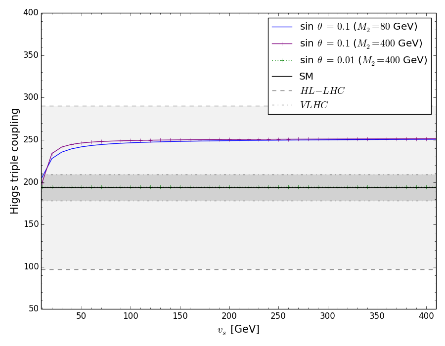
Figure 3: Higgs triple coupling $c_{111}$ as a function of $v_{s}$ for different values of $\sin\theta$ and $M_{2}$. Dashed and Dot-dashed lines represent the expected experimental precisions on $c_{111}$ at future hadron colliders, HL-LHC and VLHC, respectively LHCHiggs14 .

Due to the Higgs portal terms in Eq. 3, electroweak interaction of the Higgs boson can be significantly modified, and it is possible that $h_{1,2}$ decay into one another depending on their masses. If $M_{2}\leq M_{1}/2$, it is kinematically allowed that $h_{1}$ decays into a pair of $h_{2}$ so that the total decay width of $h_{1}$ increases. However, in this case, we found that the total decay width of $h_{1}$ exceeds too much of the currently known value of the Higgs decay width $\Gamma_{\textrm{SM}}$ = 4.07 MeV LHCHiggs13 , for any value of $\sin\theta$ unless $\lambda_{2}$ is extremely small. Therefore, we only consider a case of heavy scalar boson $h_{2}$ with mass $M_{2}>M_{1}/2$.

As well as the Higgs portal terms create new interactions between scalar bosons, they modify the Higgs self-couplings sizably. For instance, the Higgs triple coupling $c_{111}$ for $h_{1}^{3}$ interaction is given by the above model parameters as

$$c_{111}=6\lambda_{0}v_{h}\cos^{3}\theta+3(\lambda_{1}+2\lambda_{2}v_{s})\cos^{2}\theta\sin\theta+6\lambda_{2}v_{h}\cos\theta\sin^{2}\theta+(\lambda_{3}+\lambda_{4}v_{s})\sin^{3}\theta,$$ (18)

and can be probed in double Higgs production at hadron or lepton colliders. One can see from the above equation that the coupling $c_{111}$ reduces to the well-known SM value when $\theta=0$. The remaining triple-scalar couplings for $h_{1}^{2}h_{2}$, $h_{1}h_{2}^{2}$, and $h_{2}^{3}$ interactions can be found in Ref. Kim16 . In Fig. 3, we illustrate the Higgs triple coupling $c_{111}$ as a function of the scalar VEV $v_{s}$ for $\sin\theta$ = 0.1, 0.01, 0.001 and for $M_{2}$ = 80, 400 GeV. The deviation of experimental value of $c_{111}$ from the SM expectation for $\sin\theta$ = 0.1 lies within the expected precision of VLHC experiment, but not within HL-LHC precision.

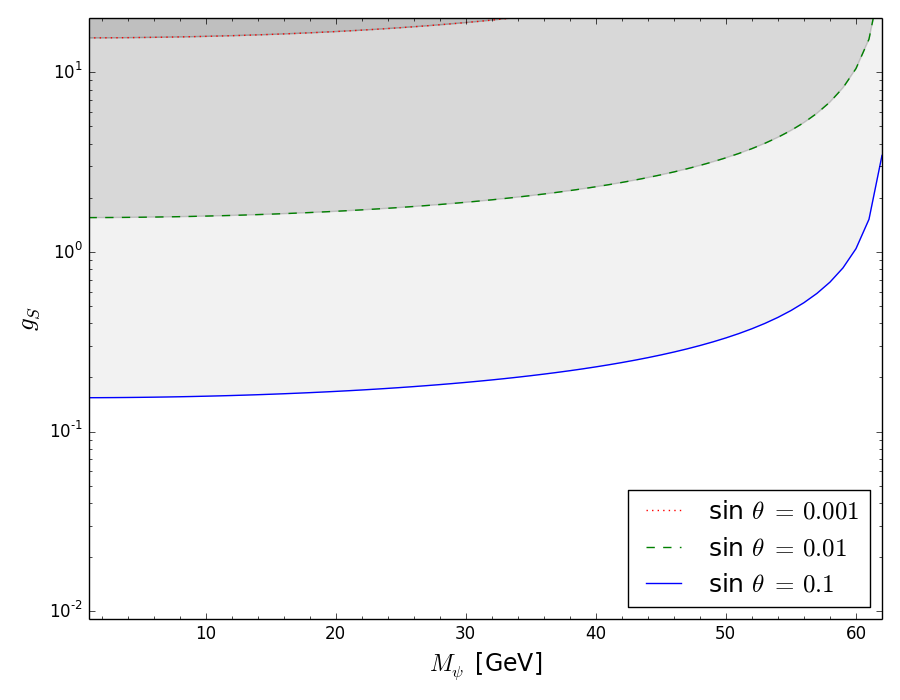
Figure 4: Shaded regions are excluded by the 90% CL limit of BR($h_{1}\to$ inv.) $<0.20$. The upper bounds are shown as different lines for three values of $\sin\theta$ = 0.1(solid blue), 0.01(dashed green), 0.001(dotted red).

If $M_{\psi}<M_{1}/2$, still, the SM Higgs $h_{1}$ can decay invisibly into a pair of DM through mixing with decay width,

$$\Gamma_{\textrm{inv.}}=\Gamma\left(h_{1}\to\psi\bar{\psi}\right)=\frac{g_{S}^{2}M_{1}\sin^{2}\theta}{8\pi}\left(1-\frac{4M_{\psi}^{2}}{M_{1}^{2}}\right)^{3/2},$$ (19)

and the corresponding branching fraction of the invisible Higgs decays is given by the relation BR($h_{1}\to$ inv.) = $\Gamma_{\textrm{inv.}}/(\Gamma_{\textrm{SM}}+\Gamma_{\textrm{inv.}})$, where $\Gamma_{\textrm{SM}}$ = 4.07 MeV LHCHiggs13 . The most recent upper limit on the Higgs invisible decay has been set by the CMS Collaboration combined with the run II data set with the luminosity of 2.3 fb^-1 at center-of-mass energy of 13 TeV CMS16 ; Higgsinv . We applied the combined 90% CL limit of BR($h_{1}\to$ inv.) $<0.20$ to our model, and depicted the result for $\sin\theta=0.1,0.01,0.001$ in Fig. 4. The bounds obtained from the invisible Higgs decays shown in Fig. 4 are not stronger than those from the DM relic density observation, and we will discuss it in the next section. Besides the invisible Higgs decays, due to the vectorial nature and degeneracy of the DM singlet fermion, the constraints coming from oblique S,T,U parameters are negligible for $\sin\theta<0.3$ (within the LEP II constraint) Chakraborty13 ; Baek12 .

V Dark Matter Phenomenology

The combined results from the recent CMB data by the Planck experiment plus WMAP temperature polarization data gives PDG14

$$\Omega_{CDM}h^{2}=0.1198\pm 0.0026.$$ (20)

This relic density observation will exclude some regions in the model parameter space. The relic density analysis in this chapter includes all possible channels of $\overline{\psi}\psi$ pair annihilation into the SM particles. In this work, we implement the model described in section 2 in the FeynRules package feynrules in order to make use of the MadGraph5 platform madgraph5 . Using the numerical package MadDM maddm2 which utilizes the MadGraph5 for computing the relevant annihilation cross sections, we obtain the DM relic density and the spin-independent DM-nucleon scattering cross sections.

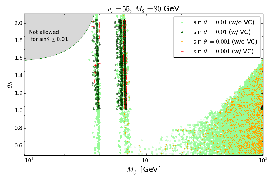
(a)

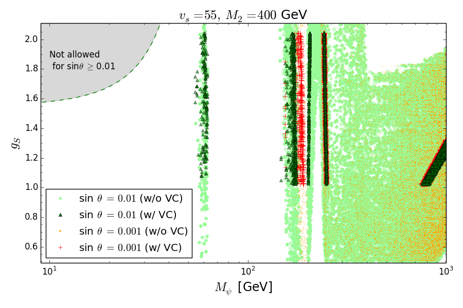
(b)

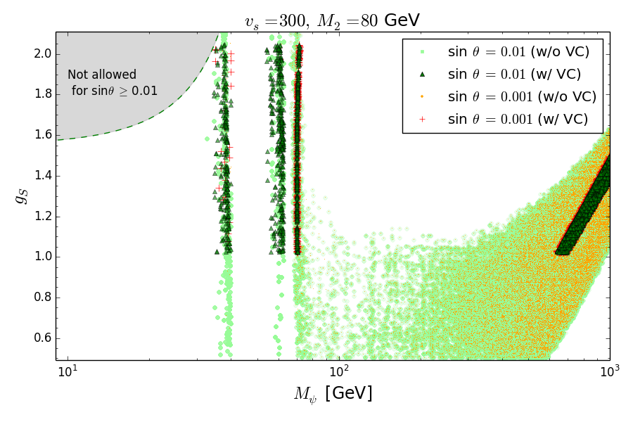
(c)

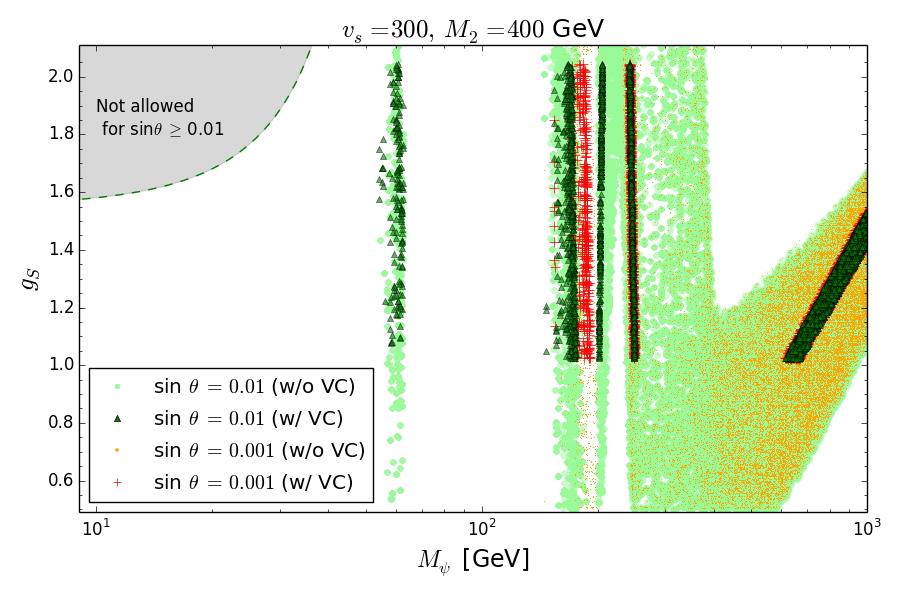
(d)

Figure 5: Allowed parameter sets of ($M_{\psi},g_{S}$) by relic density observations at $3\sigma$ level for $\sin\theta=0.01,0.001$ with and without applying the VC. The shaded area above the dashed curve indicates the exclusion limit for $\sin\theta\geq 0.01$ obtained in Fig. 4.

Instead of performing a complete analysis by varying all relevant independent NP parameters ($\sin\theta,M_{2},M_{\psi},g_{S},v_{s},\lambda_{2,4}$) in this model, we choose the benchmark points for the scalar mixing angle $\theta$, mass $M_{2}$, and VEV $v_{s}$ as follows: $\sin\theta=0.1,0.01,0.001$, $M_{2}=80,400$ GeV, and $v_{s}=55,300$ GeV as similarly considered in Ref. PMS in order to adopt the conditions on the NP parameters that lead to a strong first order phase transition as needed to produce the observed baryon asymmetry of the universe. If the VC is applied, $\lambda_{2}$ is fixed to be about 4.17 as obtained in Eq. (11), and $\lambda_{4}$ is determined by the choice of the DM coupling $g_{S}$ as in Eq. (13) which is constrained by the unitarity conditions as in Eq. (15). If only the unitarity constraints are considered without the VC, the value of the coupling $g_{S}$ is arbitrary. In order to clearly see how the VC constraints the allowed parameter space, we also scan the whole perturbative parameter region given in Eq. (14) and compare the results obtained with and without the VC applied.

For illustration of the relic density constraints on the singlet fermionic DM interaction, we first plot the allowed region of the DM mass $M_{\psi}$ and coupling $g_{S}$ constrained by the current relic density observations at $3\sigma$ level for $\sin\theta=0.01,0.001$ in Fig. 5, where four different sets of new parameters ($v_{s}$ and $M_{2}$) are chosen in the range of $0.5<g_{S}<2.11$. Without the VC constraints, of course, $g_{S}$ can possibly have a much smaller or larger value, but we don’t consider such a case which digresses from the topic of this paper. In Fig. 5, one can clearly see that the allowed DM parameter space is quite large for arbitrary values of $\lambda_{2,4}$ but much restricted to a small area once we apply the VC and the unitarity condition obtained in Eqs. (11-15). Under the VC, the allowed parameter sets are located near the resonance region of $M_{1}$ and $M_{2}$ or in the mass region of $M_{\psi}$ heavier than around 700 GeV. For different values of $\sin\theta$, the allowed parameter regions by the relic density observation are largely overlapped. For $\sin\theta=0.01,0.001$, the exclusion limits from the Higgs invisible decay shown in Fig. 4 do not give further constraints. In the case of $\sin\theta=0.1$, however, the allowed region by the relic density observation in the range of $0.5<g_{S}<2.11$ is excluded by the spin-independent DM-nucleon scattering result of recent LUX experiment as we will see later in this chapter, so we do not show the result here.

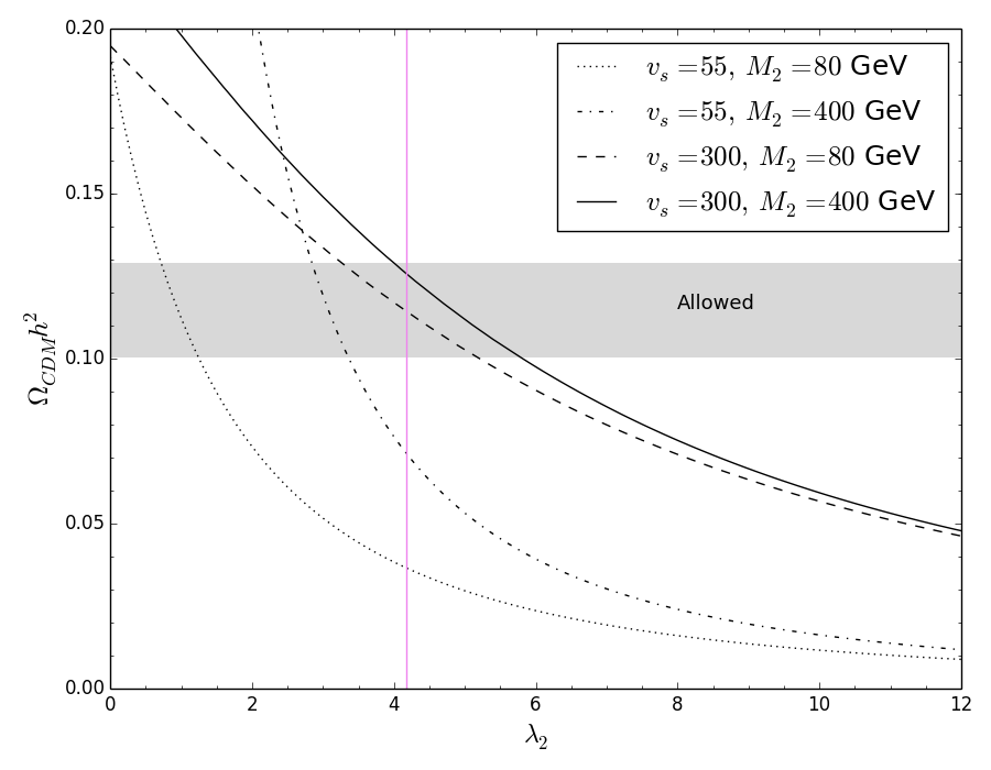
Figure 6: Relic density $\Omega_{CDM}h^{2}$ as a function of $\lambda_{2}$ for $\lambda_{4}=3.18$, $g_{S}=1.2$, $M_{\psi}=800$ GeV, and four different sets of $v_{s}$ and $M_{2}$. The vertical(violet) line indicates the VC constrained value obtained in Eq. (11), and the shaded region is allowed by the recent observation given in Eq. (20). Note that different $\sin\theta$ ($\lesssim 0.1$) doesn’t change the plots noticeably in this parameter set because $\sin\theta$ dependence is almost negligible in the heavy $M_{\psi}$ region.

In the small mass region of $M_{\psi}$ where DM pair annihilations into $h_{1}h_{2}$ and $h_{2}h_{2}$ are not kinematically allowed in the early universe, the annihilation cross section is usually quite small (for the small $\sin\theta$ and $g_{S}$ values) so that only near Higgs resonance regions annihilation cross sections can be sizable enough to have the correct DM relic density. But if the DM pair annihilations into $h_{1}h_{2}$ and $h_{2}h_{2}$ are open, then the annihilation channels can be dominant since the DM pair annihilations into $h_{1}h_{2}$ and $h_{2}h_{2}$ through s-channel $h_{2}$ mediation are not suppressed even with the small $\sin\theta$. In Fig. 5(b) and 5(d), one can clearly see that the $h_{1}h_{2}$ channel is open for $M_{\psi}\gtrsim 260$ GeV (average of $M_{1}$ and $M_{2}$) and the $h_{2}h_{2}$ channel also open for $M_{\psi}\gtrsim 400$ GeV. For the annihilation into $h_{2}h_{2}$, the annihilation diagram through t-channel $\psi$ mediation is also not suppressed with the small $\sin\theta$. The Higgs triple coupling of $h_{1}h_{2}^{2}$ interaction is given as $c_{122}=2\lambda_{2}v_{h}$ in the $\sin\theta\rightarrow 0$ limit. Therefore the annihilation cross section (in turn, the relic density) dependence on $\lambda_{2,4}$ becomes more important in the heavy $M_{\psi}$ region. In Fig. 6, we show the relic density as a function of $\lambda_{2}$ for $\lambda_{4}=3.18$, $g_{S}=1.2$, $M_{\psi}=800$ GeV, and four different sets of $v_{s}$ and $M_{2}$. As $\lambda_{2}$ grows, the Higgs triple coupling $c_{122}$ gets larger so that the annihilation cross section gets larger and in turn the relic density gets smaller. Therefore, if $\lambda_{2}$ is a free parameter we can adjust the $\lambda_{2}$ value to have a correct DM relic density. However, with the VC imposed, we do not have such freedom (here $\lambda_{2}$ is fixed as 4.17) and therefore only limited parameter sets are survived.

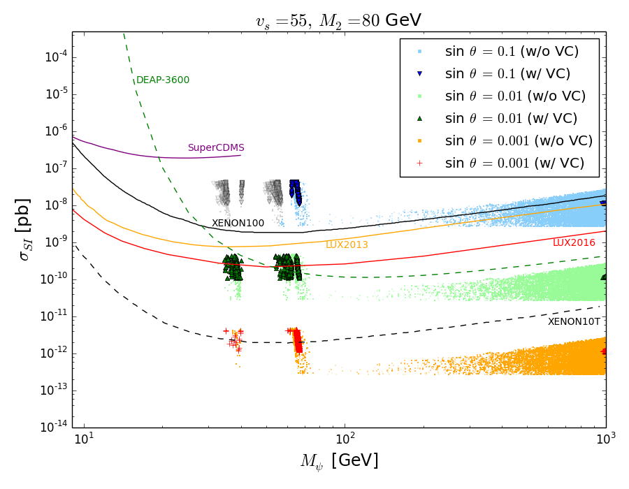
(a)

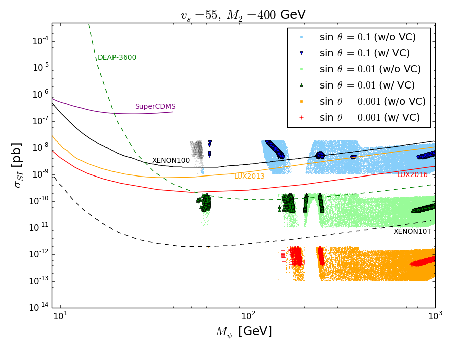
(b)

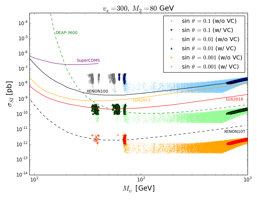
(c)

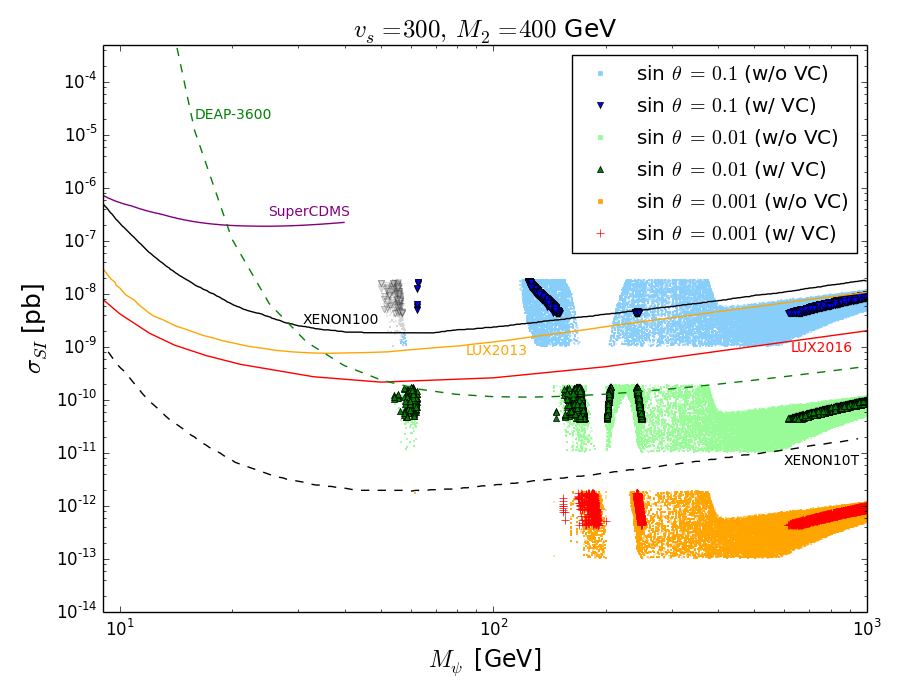
(d)

Figure 7: Spin-independent DM-nucleon scattering results allowed by relic density observations for $0.5<g_{S}<2.11$ with and without applying the VC. Also shown are observed limits from LUX 2013, 2016, XENON100, SuperCDMS, and expected limits from DEAP-3600 and XENON10T. For $\sin\theta=0.1$, some of allowed parameter sets by the relic density observation in low DM mass (grayed) region are excluded by the invisible Higgs decay bound given in Fig. 4.

In Fig. 7, we plot the spin-independent DM-nucleon scattering cross section by varying the DM mass $M_{\psi}$ with parameter sets allowed by the relic density observation, and compare the results with the observed upper limits obtained at 90$\%$ level from LUX 2013, 2016, XENON100, SuperCDMS, and with the expected limits from DEAP-3600 and XENON10T. One can see from the figure that $\sin\theta\gtrsim 0.1$ case obtained in the range of $0.5<g_{S}<2.11$ is not favored in this model due to the recent LUX bound LUX16 , and most of allowed regions for $\sin\theta=0.01,0.001$ are not excluded. Also, $\sin\theta=0.01$ scenario can be tested sooner or later by ongoing experiments such as XENON10T.

If one chooses the second scenario ($\lambda_{2}(v)=2.0$) instead of the first scenario ($\lambda_{2}(v)=4.17$), the allowed regions for $M_{\psi}>600$ GeV with the VC applied in Fig. 5 and 7 will be shifted a bit but not much, and still be inside of the allowed regions obtained generally without the VC. Similarly, even if one introduces additional NP in the hidden sector at a TeV scale and apply the VC at the NP scale, our numerical results can still be applicable and provide meaningful guidelines as discussed in Sec. III.

VI Concluding Remarks

In this paper, we studied the renormalizable Higgs portal model of a fermionic dark matter with a gauge singlet Dirac fermion and a real single scalar which ensure the cancellation of one-loop quadratic divergence to the Higgs and the additional singlet scalar masses. We showed that our DM model can satisfy the VCs for the quadratic divergences to the masses of the SM-like Higgs boson and the singlet scalar simultaneously. We constrained the Higgs-scalar coupling $\lambda_{2}$ and the scalar self-interaction coupling $\lambda_{4}$ using the VC. We further constraint those couplings using the perturbative unitarity conditions, and obtained the bound on the DM coupling $g_{S}$ as well.

We showed the allowed region of NP parameters, the DM mass $M_{\psi}$ and coupling $g_{S}$, satisfying the recent measurement of relic abundance with and without the VC constraints in Fig. 5. We also showed the spin-independent DM-nucleon scattering cross section of the singlet fermionic DM by varying the DM mass $M_{\psi}$ with parameter sets allowed by the relic density observation, and compare the results with the observed upper limits from various experiments in Fig. 7. In the figures, one can clearly see that the allowed parameter space constrained by the VC are located near the resonance region of $M_{1}$ and $M_{2}$ or in the mass region of $M_{\psi}$ heavier than about 700 GeV. We performed the numerical analysis for three different values of the Higgs-scalar mixing angle $\sin\theta=0.1,0.01,0.001$, and the $\sin\theta=0.1$ case is disfavored in this model due to the recent LUX bound even in the case without the VC applied.

Our renormalizable DM model with a singlet Dirac fermion and a real single scalar is a minimal DM model which has allowed NP parameter space where the fine-tuning (or the hierarchy) problem of the Higgs mass is much relaxed, and this model can be expanded by introducing complex scalars and/or DM fermion multiplets. The obtained allowed parameter sets under the VC can be used as benchmark points to test proper DM model candidates as future experimental progress can further improve the bounds.

- (1) G. Aad et al., ATLAS Collaboration, Phys. Lett. B 716, 1 (2012).
- (2) S. Chatrchyan et al., CMS Collaboration, Phys. Lett. B 716, 30 (2012).
- (3) B.W. Lee, C. Quigg, and H.B. Thacker, Phys. Rev. D 16, 1519 (1977); W. Marciano, G. Valencia, and S. Willenbrock, Phys. Rev. D 40, 1725 (1989).
- (4) M. Veltman, Acta Phys. Polon. B12 (1981) 437.
- (5) L. Susskind, Phys. Rev. D 20, 2619 (1979).
- (6) H. Georgi, H. Quinn, and S. Weinberg, Phys. Rev. Lett. 33, 451 (1974).
- (7) J.F. Gunion, arXiv:0804.4460 [hep-ph].
- (8) B. Grzadkowski and J Wudka, Phys. Rev. Lett. 103, 091802 (2009); B. Grzadkowski and J Wudka, Acta Phys. Polon. B40 (2009) 3007.
- (9) G.B. Pivovarov and V.T. Kim, Phys. Rev. D 78, 016001 (2008).
- (10) I. Masina and M. Quiros, Phys. Rev. D 88, 093003 (2013).
- (11) C.N. Karahan and B. Korutlu, Phys. Lett. B 732, 320 (2014).
- (12) D.A. Demir, C.N. Karahan, and B. Korutlu, Phys. Lett. B 740, 46 (2015).
- (13) A. Drozd, B. Grzadkowski, and J. Wudka, J. High Energy Phys. 04, 006 (2012).
- (14) I. Chakraborty and A. Kundu, Phys. Rev. D 87, 055015 (2013).
- (15) Y.G. Kim and K.Y. Lee, Phys. Rev. D 75, 115012 (2007); K.Y. Lee, Y.G. Kim, and S. Shin, J. High Energy Phys. 05, 100 (2008).
- (16) S. Profumo, M.J. Ramsey-Musolf and G. Shaughnessy, J. High Energy Phys. 0708, 010 (2007).
- (17) Y.G. Kim, K.Y. Lee, C.B. Park, and S. Shin, Phys. Rev. D 93, 075023 (2016).
- (18) M.S. Al-sarhi, I. Jack, and D.R.T. Jones, Z. Phys. C 55, 283 (1992).
- (19) G. Cynolter, E. Lendvai, and G. Pócsik, arXiv:0410102 [hep-ph]; F. Kahlhoefer and J. McDonald, JCAP 11, 015 (2015).
- (20) S. Baek, P. Ko, W.-I. Park, and E. Senaha, J. High Energy Phys. 11, 116 (2012).
- (21) R. Barbieri and A. Strumia, Phys. Lett. B 462, 144 (1999).
- (22) C. Kolda and H. Murayama, J. High Energy Phys. 07, 035 (2000).
- (23) LHC Higgs Cross Section Working Group Collaboration, arXiv:1307.1347 [hep-ph].
- (24) A. Ajaib et al., arXiv:1310.8361 [hep-ph].
- (25) CMS Collaboration, CMS PAS HIG-16-016.
- (26) G. Aad et al., ATLAS Collaboration, J. High Energy Phys. 11, 206 (2015).
- (27) K.A. Olive et al., Particle Data Group, Chin. Phys. C 38, 090001 (2014).
- (28) A. Alloul et al., Comput. Phys. Commun. 185, 2250 (2014).
- (29) J. Alwall et al., J. High Energy Phys. 07, 079 (2014).
- (30) M. Backovic et al., Phys. Dark Univ. 9-10, 37 (2015).
- (31) D.S. Akerib et al., LUX Collaboration, Phys. Rev. Lett. 118, 021303 (2017).