HelMod in the works: from direct observations to the local interstellar spectrum
of cosmic-ray electrons

Abstract

The local interstellar spectrum (LIS) of cosmic-ray (CR) electrons for the energy range 1 MeV to 1 TeV is derived using the most recent experimental results combined with the state-of-the-art models for CR propagation in the Galaxy and in the heliosphere. Two propagation packages, GALPROP and HelMod, are combined to provide a single framework that is run to reproduce direct measurements of CR species at different modulation levels, and at both polarities of the solar magnetic field. An iterative maximum-likelihood method is developed that uses GALPROP-predicted LIS as input to HelMod, which provides the modulated spectra for specific time periods of the selected experiments for model-data comparison. The optimized HelMod parameters are then used to adjust GALPROP parameters to predict a refined LIS with the procedure repeated subject to a convergence criterion. The parameter optimization uses an extensive data set of proton spectra from 1997–2015. The proposed CR electron LIS accommodates both the low-energy interstellar spectra measured by Voyager 1 as well as the high-energy observations by PAMELA and AMS-02 that are made deep in the heliosphere; it also accounts for Ulysses counting rate features measured out of the ecliptic plane. The interstellar and heliospheric propagation parameters derived in this study agree well with our earlier results for CR protons, helium nuclei, and anti-protons propagation and LIS obtained in the same framework.

1. Introduction

Electrons in the cosmic radiation were identified for the first time about fifty years after the discovery of CRs (Meyer & Vogt, 1961; Earl, 1961). Subsequently, the origin of the observed spectrum of CR electrons has been one of the most important questions in CR physics. Early CR electron measurements of increasing precision and expanding energy range were made over a series of balloon flights by different experiments (e.g., Fanselow et al., 1969; Buffington et al., 1975; Hartman & Pellerin, 1976; Golden et al., 1984, 1994; Basini et al., 1995; Barwick et al., 1998; Boezio et al., 2000; Torii et al., 2001; Grimani et al., 2002). However, the experimental scatter was large because the CR electron spectrum is steeply falling with increasing energy, and the background of heavier CR species is high.

The first high-statistics measurements of the all-electron CR spectrum over a wide energy range were made by the Fermi Large Area Telescope (Fermi–LAT) launched in 2008 (Atwood et al., 2009). These measurements showed that the all-electron spectrum is flatter than expected with an index about –3 over the energy range 7–1000 GeV (Abdo et al., 2009; Ackermann et al., 2010). PAMELA data (1–625 GeV, Adriani et al., 2011) generally confirmed the Fermi–LAT results albeit with larger error bars, as did the higher precision data from AMS-02 (0.5-1000 GeV, Aguilar et al., 2014a). Even though the precise AMS-02 data showed deviations from the earlier Fermi–LAT measurements that are significant due to high statistics and consequently very small error bars, the absolute difference is only $\sim$10% above 20 GeV vs. a factor of $\sim$3–4 in the pre-Fermi era. Note that the latest Fermi–LAT all-electron spectrum (7–2000 GeV) obtained using a revised event reconstruction and background rejection analysis (Abdollahi et al., 2017) agrees well with AMS-02 results. Above $\sim$1 TeV, the all-electron spectrum falls rapidly (H.E.S.S., Aharonian et al., 2008, 2009). The first ever measurement of the all-electron spectrum for energies $\lesssim 100$ MeV outside of the heliosphere has been made by Voyager 1 that reached the heliopause in 2012 (Stone et al., 2013; Cummings et al., 2016).

The strong interest in the CR electron spectrum during the last decade is also fueled by the PAMELA discovery of a continuous rise of the positron fraction up to $\sim 100$ GeV (Adriani et al., 2009), and expectations of spectral features at very-high energies associated with local CR accelerators (e.g., Kobayashi et al., 2004). The latter are yet to be found, although the dedicated experiment CALET has been operating on the International Space Station (ISS) since August 19, 2015 (Asaoka et al., 2017), and the ISS-CREAM, which was launched to the ISS on August 14, 2017, is also deployed there to make CR measurements in the multi-TeV range (Seo et al., 2014).

The discovery of the rise of the positron fraction by PAMELA, contrary to the expectations based on the pure secondary production of positrons in energetic CR interactions with the interstellar gas (Protheroe, 1982; Moskalenko & Strong, 1998), was the first clear evidence of new phenomena detected in CRs, even though the first hints of it appeared in data collected by earlier experiments. The TS93 apparatus launched on a balloon from Fort Sumner, NM, in 1993 measured a flat positron fraction $0.078\pm 0.016$ in the range $\sim$5–60 GeV (Golden et al., 1996). Subsequent balloon-borne flights by CAPRICE94 in 1994 (Boezio et al., 2000), the HEAT-$e^{\pm}$ instrument in 1994 and 1995 (Barwick et al., 1997), and HEAT-pbar instrument in 2000 (Beatty et al., 2004), indicated that the positron flux did not fall-off as quickly as expected. However, the experimental error bars in these early experiments were too large to provide convincing evidence for a new phenomenon.

Following the PAMELA discovery the rise of the positron fraction up to 200 GeV was confirmed by the Fermi–LAT (Ackermann et al., 2012a), where the geomagnetic field (the “East-West effect”) was used to provide the charge sign separation, and then up to $\sim 500$ GeV with higher precision by AMS-02 (Accardo et al., 2014; Aguilar et al., 2014a). These measurements stimulated an extensive discussion of the origin of the rising positron fraction with dozens of different hypotheses proposed in the literature. They range from conventional astrophysics to non-standard model physics involving various types of dark matter particles. A component with similar origin could be also present in the electron spectrum (e.g., Della Torre et al., 2015).

High-precision measurements of both electrons and positrons over a wide energy range are thus of critical importance toward unveiling the origin of the excess positrons. Meanwhile, the $e^{\pm}$ spectra and the positron fraction below $\sim$10 GeV was found to depend on the solar activity (PAMELA, Adriani et al., 2016). The determination of the true electron LIS is, therefore, of considerable interest for the astrophysics and particle physics communities. In the present paper, the same method – including the treatment of errors – is employed as for the recently published studies devoted to the LIS of CR protons, helium nuclei, and anti-protons (Boschini et al., 2017a).

2. GALPROP and HelMod codes

In this paper, we use a recently developed version of the HelMod 2D Monte Carlo code for heliospheric CR propagation (Bobik et al., 2012, 2013; Boschini et al., 2017b) combined with the GALPROP code for interstellar CR propagation (Jóhannesson et al., 2016; Porter et al., 2017) to take advantage of the progress made in the recent CR electron measurements and to derive a self-consistent electron LIS. The HelMod code includes all relevant effects and, thus, a full description of the diffusion tensor. HelMod enables accurate calculations for the heliospheric modulation effect over arbitrary epochs and is easily interfaced with GALPROP.

2.1. Galactic CR propagation with the GALPROP code

The GALPROP code has been under development since the mid-90s (Moskalenko & Strong, 1998; Strong & Moskalenko, 1998) and is the de facto standard code for calculating the propagation of CRs and their associated interstellar emissions. It solves the CR transport equation for a given source distribution and boundary conditions for all CR species. GALPROP includes all relevant transport and energy loss/gain processes, such as a galactic wind (advection), diffusive reacceleration in the ISM, energy losses, nuclear fragmentation, radioactive decay, and the production of secondary particles and isotopes. The numerical solution of the transport equation can be obtained using different solvers, including a Crank-Nicholson implicit second-order scheme as well as an explicit method. The spatial boundary conditions assume free particle escape. For a given halo size the diffusion coefficient as a function of momentum is determined by fitting model parameters to CR nuclei secondary-to-primary ratios.

The GALPROP code computes a full network of CR primary, secondary and tertiary species from input source abundances. Starting with the heaviest primary nucleus typically considered (⁶⁴Ni, $A=64$) the propagation solution is used to compute the source term for its spallation products $A-1$, $A-2$, and so forth. These are propagated in turn, and so on down in mass to protons, secondary $e^{\pm}$, and $\bar{p}$. The inelastically scattered $p$ and $\bar{p}$ are treated as separate components (secondary $p$, tertiary $\bar{p}$). GALPROP includes a description for the processes of K-capture, electron capture by bare CR nuclei and stripping, as well as knock-on electrons. More details are given in Ptuskin et al. (2006), Strong et al. (2007), Vladimirov et al. (2011), and Jóhannesson et al. (2016), as well as the description of the most recent version of GALPROP (v. 56) – see Moskalenko et al. (2017) and Porter et al. (2017), and references therein.

2.2. HelMod code for heliospheric CR transport

GALPROP provides the predictions for the LIS of all CR species. However, they cannot be compared to the direct CR measurements made at Earth’s orbit, or generally in the inner heliosphere, because of the effect of the so-called heliospheric or solar modulation. This modulation is the combined effect of the expanding magnetic fields and the solar wind (SW) whose properties depend on the level of solar activity (e.g., see Boschini et al., 2017a, b).

The propagation of CRs in the heliosphere was first studied by Parker (1965), who formulated the transport equation (also called the Parker equation – see, e.g., the discussion in Bobik et al., 2012, and reference therein):

$$\frac{\partial U}{\partial t}= \frac{\partial}{\partial x_{i}}\left(K^{S}_{ij}\frac{\partial\mathrm{U}}{\partial x_{j}}\right)$$ (1)

$$+\frac{1}{3}\frac{\partial V_{\mathrm{sw},i}}{\partial x_{i}}\frac{\partial}{\partial T}\left(\alpha_{\mathrm{rel}}T\mathrm{U}\right)-\frac{\partial}{\partial x_{i}}[(V_{\mathrm{sw},i}+v_{d,i})\mathrm{U}],$$

where $U$ is the number density of Galactic CR particles per unit of kinetic energy $T$ (GeV/nucleon), $t$ is time, $V_{\mathrm{sw},i}$ is the SW velocity along the axis $x_{i}$, $K^{S}_{ij}$ is the symmetric part of the diffusion tensor, $v_{d,i}$ is the particle magnetic drift velocity (related to the anti-symmetric part of the diffusion tensor), and $\alpha_{\mathrm{rel}}=\frac{T+2m_{r}c^{2}}{T+m_{r}c^{2}}$, with $m_{r}$ – the particle rest mass per nucleon in units of GeV/nucleon. The terms in the Parker equation describe: (i) the diffusion of Galactic CRs scattered by magnetic turbulences, (ii) the adiabatic energy losses/gains due to the propagation in the expanding magnetic fields carried in the SW, (iii) an effective convection resulting from the SW convection with velocity $\vec{V}_{\rm sw}$, and (iv) the drift effects related to the drift velocity ($\vec{v}_{\rm drift}$). Overall, the heliospheric modulation results in energy losses and supression of the fluxes of CR species compared to the LIS that are energy- and charge-sign-dependent. These effects are controlled by the polarity of the solar magnetic field and by the level of solar activity.

The particle transport within the heliosphere, from the Termination Shock (TS) to Earth’s orbit, is treated in this paper using the HelMod code. HelMod integrates the Parker (1965) transport equation using a Monte Carlo approach involving stochastic differential equations; for further details of the method and code see Bobik et al. (2012, 2016).

In previous models of CR propagation in the heliosphere, the parallel diffusion coefficient ($K_{||}$) was assumed to have a sharp break at $\sim$1 GV, in the transitional region between the two regimes at high and low rigidities (e.g., see Perko, 1987; Alanko-Huotari et al., 2007; Strauss et al., 2011; Bobik et al., 2012). However, as the accuracy of the collected data increased, it becomes clear that a smooth transition between the two regimes is necessary. The functional form of such a transition that is currently employed in HelMod (see Equation 5 in Boschini et al., 2017b) is consistent with those presented in Burger & Hattingh (1998) for the same rigidity interval.

The normalization of the parallel component $K_{||}$ of the symmetric part of the diffusion tensor $K^{S}_{ij}$ is determined by the so-called diffusion parameter $K_{0}$, as defined by Eq. (2) of Boschini et al. (2017b, and references therein). In turn, the diffusion parameter $K_{0}$ includes a correction factor that rescales the absolute value proportionally to the drift contribution. This correction factor is evaluated in Boschini et al. (2017a) using the proton spectrum during the period of positive polarity of the heliospheric magnetic field (HMF), and accounts for the presence of the latitudinal structure in the spatial distribution of Galactic CRs. The same correction factor is now applied to electron propagation ($q<0$) during the negative HMF polarity period ($A<0$), so that an equivalent scaling is applied to periods with $qA>0$.

The drift treatment in HelMod follows the formalism originally developed by Potgieter & Moraal (1985) and refined using Parker’s magnetic field with polar correction described in Bobik et al. (2013). During high activity periods the heliospheric magnetic field is far from being considered regular, therefore, we introduced a correction factor suppressing any drift velocity at solar maximum.

As discussed by Boschini et al. (2017b), the validity of the HelMod code is verified down to about 1 GV rigidities (equivalent to $\sim$1 GeV in kinetic energy for electrons). Lower rigidities/energies are not considered in the present work because to do so requires additional refinement for the description of the solar modulation in the outer heliosphere – between TS and interstellar space (see, e.g., Scherer et al., 2011; Dialynas et al., 2017) – as well as inclusion of the turbulence in the calculation of the drift coefficient (see, e.g., Engelbrecht et al., 2017). However, Voyager 1 electron data is used as a guideline.

Table 1Best-fit propagation parameters for electrons

N	Parameter		Best Value
1	$z_{h}$,	kpc	4.0
2	$D_{0}$,	$10^{28}$ cm2 s-1	4.3
3	$\delta$		0.405
4	$V_{\rm Alf}$,	km s-1	31
5	$dV_{\rm conv}/dz$,	km s-1 kpc-1	9.8

Table 2Electron injection spectrum

Parameters	Values
$R_{0}$	190 MV
$R_{1}$	6 GV
$R_{2}$	95 GV
${\gamma}_{0}$	2.57
${\gamma}_{1}$	1.40
${\gamma}_{2}$	2.80
${\gamma}_{3}$	2.40/2.54

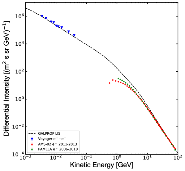
Figure 1.— The electron LIS (dashed) as derived from the MCMC procedure compared with AMS-02, PAMELA and Voyager 1 measurements (see text).

3. Interstellar propagation

The tuning procedure employed in this paper is the same that was used by Boschini et al. (2017a). A short description of the method is provided below.

The Markov Chain Monte Carlo (MCMC) interface to v.56 of GALPROP was adapted from CosRayMC (Liu et al., 2012) and, in general, from the COSMOMC package (Lewis & Bridle, 2002). An iterative procedure was developed that calculates LIS with GALPROP, passing the results to HelMod to produce the modulated spectra for specific time periods for comparison with AMS-02 data, which are the observational constraints. The goodness estimator of the parameter scan is the natural logarithm of the likelihood. For computational convenience this is built using $\chi^{2}$ from all observables: hundreds of thousands of samples were generated and the Log-Likelihood used to accept or reject each sample. The scan is terminated when the Log-Likelihood is maximized.

The basic features of CR propagation in the Galaxy are well-known, but the exact values of propagation parameters depend on the assumed propagation model and accuracy of selected CR data. Therefore, the MCMC procedure is used to determine the propagation parameters employing the best available CR measurements. The five propagation parameters that have the largest effect on the overall shape of CR spectra were left free in the scan that used a 2D GALPROP model: the Galactic halo half-width $z_{h}$, the normalization of the diffusion coefficient $D_{0}$ and the index of its rigidity dependence $\delta$, the Alfvén velocity $V_{\rm Alf}$, and the gradient of the convection velocity $dV_{\rm conv}/dz$ ($V_{\rm conv}=0$ in the plane, $z=0$). The spatial distribution of CRs near the Sun depends only weakly on the chosen radial size of the Galaxy if its distance is farther than the halo size (e.g., Ackermann et al., 2012b). The radial boundary is therefore set to 20 kpc.

The best values for the main propagation parameters tuned to the AMS-02 data are listed in Table 1. The values are similar to those obtained by Boschini et al. (2017a), within the quoted error bands, while the convection velocity $V_{\rm conv}$ is set to 0 in the plane. For example, to get a more consistent electron LIS, the Alfvén velocity $V_{\rm Alf}$ was increased by $\sim 2$ km s^-1. As already discussed by Boschini et al. (2017a), simultaneous inclusion of both reacceleration and convection is needed to describe the high precision AMS-02 data, particularly in the range below 20 GV where the modulation effects on CR spectra are significant. For more details the reader is referred to the above-mentioned paper.

The MCMC procedure is used only for first step to define a consistent set for the Galactic CR propagation parameters. The HelMod module was then used for a methodical calibration of the LIS spectral parameters. Parameters of the injection spectra, such as spectral indices $\gamma_{i}$ and the break rigidities $R_{i}$, were left free, but their exact values depend on the solar modulation, so the low-energy parts of the spectra are tuned together with the solar modulation parameters as described below.

To refine the LIS description smoothing features to the breaks in the injection spectrum were added. Reproducing the electron spectrum from MeV to TeV energies requires an injection spectrum with three spectral breaks. MCMC scans in $\gamma_{i}$ and $R_{i}$ were performed using CR electron measurements by AMS-02 (Aguilar et al., 2014b) and by Voyager 1 (Cummings et al., 2016) as constraints. At the next step, these parameters were slightly modified together with the solar modulation parameters in order to find the best-fit solution for the electron LIS, as explained by Boschini et al. (2017a). Reproduction of the low-energy electron LIS measurements by Voyager 1 requires a break around $R_{0}\sim 190$ MV. The resulting best-fit spectral parameters are shown in Table 2.

Note that the only data available to tune the electron LIS below AMS-02 energies are coming from Voyager 1. Unfortunately, the Electron Telescope (TET) aboard the Voyager 1 spacecraft cannot discriminate between electrons and positrons, so it provides only the all-electron spectrum. On the other hand, GALPROP calculations indicate that the secondary positron fraction decreases as energy decreases being $\lesssim 35$% at its maximum contribution for $\sim 200$ MeV energies, and becomes as small as a few per cent or less below $\sim$20 MeV (e.g., Porter et al., 2008). Therefore, assuming that only electrons are present in CRs at low energies the maximum error in the results at these energies would be $\sim 30$%.

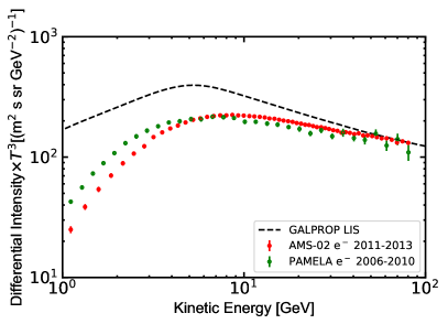
Figure 2.— The proposed electron LIS is compared with high-energy all-electron data from AMS-02 and PAMELA experiments.

Table 3Normalization corrections applied to the electron LIS

Dataset group	Experiment	Time span	Normalization correction	Reference
a)	PAMELA	5 years integrated spectrum	0.81	Adriani et al. (2011)
b)	PAMELA	6 months integrated spectrum	0.9	Adriani et al. (2015)
c)	AMS-02	3 years integrated spectrum	1.0	Aguilar et al. (2014b)

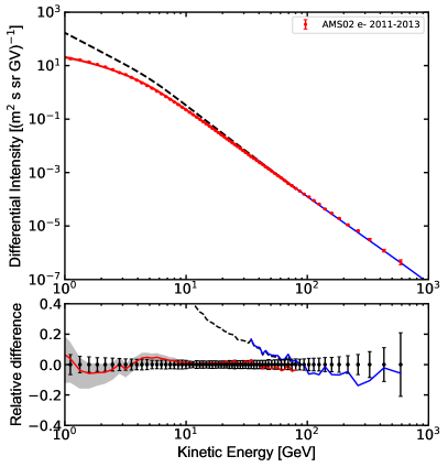
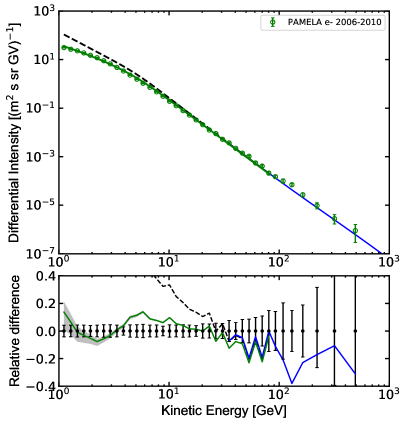
Figure 3.— Differential intensity of CR electrons for AMS-02 2011-2013 (left) and PAMELA 2006-2010 (right) datasets. Points represent experimental data, the black dashed line is the GALPROP LIS, and the red/green solid lines are the computed modulated spectra. The blue solid line represents the expected LIS including the high energy electron excess contribution (see text). The bottom panel shows the relative difference between the numerical solutions and the experimental data.

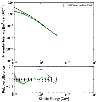
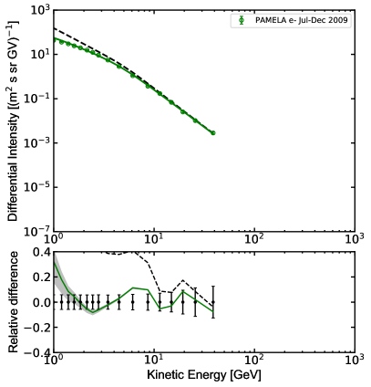
Figure 4.— Differential intensity of CR electrons for PAMELA 2006 (left) and PAMELA 2009 (right) datasets. Points represent experimental data, the black dashed line is the GALPROP LIS, and green solid lines are the computed modulated spectra. The bottom panel shows the relative difference between the numerical solution and the experimental data.

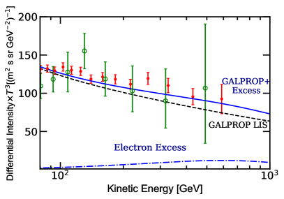
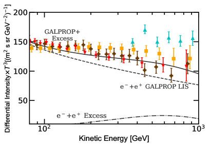
Figure 5.— High energy LIS for electrons (left panel) and “all-electrons” (right panel) along with AMS-02 (red points, Aguilar et al. 2014b, a), PAMELA (green open circles, top panel, Adriani et al., 2011), Fermi-LAT (orange squares, bottom panel, Ackermann et al. 2012a), CALET (brown crosses, bottom panel, Adriani et al. 2017) and H.E.S.S. (cyan triangles, bottom panel, Aharonian et al. 2008) measurements. The GALPROP LIS is plotted with the dashed line, the estimated high-energy omindirectional-intensity positron excess is plotted with the dot-dash line (multiplied by a factor of 2 in the bottom panel to account for the identical electron excess, see text) and, finally the sum of GALPROP LIS and electron and positron excess components is plotted with the solid line.

3.1. Electron LIS at low and Intermediate energies

Since the end of August, 2012, the Voyager 1 mission is exploring interstellar space providing invaluable data on the composition of Galactic CRs at low energies (Stone et al., 2013; Cummings et al., 2016). In the current analysis Voyager 1 data (Cummings et al., 2016) taken between December 2012 and June 2015 is used as a constraint for evaluating the electron LIS, as described above. A comparison of the Voyager 1 all-electron spectrum in the kinetic energy range 3–74 MeV and the proposed model for the LIS is shown in Figure 1. The combined model provides a good description of the electron LIS at low energies.

At high energies, where the CR fluxes are not affected by the heliospheric modulation, the most recent measurements by AMS-02 and PAMELA up to 90 GeV are included and shown in Figure 2. The electron LIS at even higher energies is discussed in Sect. 4.

It can be seen that even though the AMS-02 (Aguilar et al., 2014b) and PAMELA data (Adriani et al., 2011) in Figure 2 are consistent within the error bars, the systematic difference between the datasets can be as large as $\sim$20% in the energy range 30–90 GeV. Speculation on the possible origin(s) of this difference is not made here. However, it is clear that it is not the effect of solar modulation because it should be insignificant at these energies. For the MCMC procedure (Sect. 2.1) the AMS-02 data is used because it has the smallest error bars.

3.2. Data at Earth and outside of the ecliptic plane

This section illustrates an application of the HELMOD code to derivation of the modulated electron spectra at Earth. The spectra have to be compared to those measured by AMS-02 and PAMELA during periods of low (i.e., PAMELA from 2006 to 2010, Adriani et al., 2011, 2015) and high solar activity (i.e., AMS-02 from 2011 to 2013, Aguilar et al., 2014b). The available data are integrated over a period of a few months to years. To reproduce the conditions of both low and high solar activity, the HelMod modulated spectra are evaluated for each Carrington Rotation within the period appropriate to the corresponding dataset. The obtained results are then used to evaluate a unique normalized probability function for the modulation tool described in Section 3.1 of Boschini et al. (2017a).

Improvements in the data analysis procedure and in the simulation of the time dependence of the tracking system performance of PAMELA (Adriani et al., 2015) lead to a $\sim$10% increase in the overall normalization of the CR electron fluxes measured in the period from July, 2006 – December, 2009 compared to earlier results (Adriani et al., 2011). However, it is not enough to account for a systematic discrepancy of $\sim$20% between AMS-02 and earlier results from PAMELA (Adriani et al., 2011). Due to the smaller quoted systematic uncertainties, the AMS-02 data are used as the reference. In this work a normalization factor for the electron LIS that is listed in Table 3 is calculated for each presented dataset.

The computed modulated spectra, for both low and high solar activity periods, are shown in Figures 3 and 4. The details of the modulation model are described in Sect. 2.2 and applied to the LIS described in Sect. 3.1. The high energy part of the spectrum is not affected by the solar modulation, and, therefore, is not discussed here. Simulated spectra are in a good agreement with experimental data in the energy range from 1 GeV to 90 GeV. The $\sim 2\sigma$ deviations seen in the energy range $\lesssim$3 GeV are present in all spectra, and this most likely implies that the injection spectrum needs some additional adjustments. Further comparison with the data is made in Appendix A that also includes data taken by PAMELA around solar minimum (Adriani et al., 2015).

A reliable model for heliospheric modulation requires a proper modeling of CR distribution in the whole heliospheric volume, including space outside the ecliptic plane and at large distances from the Sun. Since 1990s and until 2009, the Ulysses spacecraft (see e.g. Sanderson et al., 1995; Marsden, 2001; Balogh et al., 2001) explored the heliosphere outside the ecliptic plane up to $\pm 80^{\circ}$ in solar latitude and at distances $\sim$1–5 AU from the Sun. In particular, observations of particle flux were performed using the Cosmic Ray and Solar Particle Investigation Kiel Electron Telescope (COSPIN/KET) and High Energy Telescope (COSPIN/HET). Figure 6 shows the Ulysses counting rate normalized to the average value. Data for Ulysses were taken from Ulysses Final Archive. The analyzed data come from the KET electron channel E300-B (Rastoin et al., 1996, electron energies of 0.9–4.6 GeV) using the Carrington Rotation average.

HelMod calculations are made for electrons of 0.6–10 GeV for each Carrington Rotation at the same distance and solar latitude as the Ulysses spacecraft. In order to correctly weight the spectral energy distribution, the calculated differential flux is then convolved with the subchannel response function available in Rastoin et al. (1996). The error band was evaluated using the procedure described in Boschini et al. (2017a). Figure 6 shows a comparison of the Ulysses data with the HelMod calculations. Both experimental data and simulations are normalized to their corresponding mean values to allow a relative comparison along the solar cycle. The model reproduces the general features of the latitudinal gradients observed during the fast scans of 1994–1995 and 2007. Moreover, the agreement is still acceptable along the whole orbit, which extends as far as $\sim$3 AU. We note that the purpose of Figure 6 is only to demonstrate the qualitative agreement between the HelMod calculations and observations. A proper quantitative comparison with the Ulysses data would require a calculation that combines several energy bins weighted with the Ulysses response function and detector efficiency.

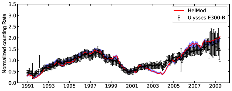
Figure 6.— Ulysses counting rate normalized to the average value for the KET electron channel E300-B (electron energies of 0.9–4.6 GeV) as a function of time, where each point is an average over one Carrington rotation. The red solid line is the HelMod calculation for electrons of 0.6–10 GeV convolved with the subchannel response function for each Carrington rotation at same distance and solar latitude of the Ulysses spacecraft. Blue area shows systematic errors associated with model calculations.

4. Electron LIS

In addition to the plots and tabulated data presented in Sect. 3.2 and the Appendix, we provide a parameterization $F(T)$ of the GALPROP LIS (Figure 1) from 2 MeV up to 90 GeV as a function of kinetic energy in GeV:

T<6.88 GeV995.598T−3.505+4.423T−2.620, T≥6.88 GeV\displaystyle\left\{\begin{tabular}[]{lr}\lx@intercol$\displaystyle\frac{1.181\!\!\times\!\!10^{11}T^{-12.061}}{1+4.307\!\!\times\!\!10^{8}T^{-9.269}+3.125\!\!\times\!\!10^{8}T^{-10.697}}$,\hfil\lx@intercol\\ &$T<6.88$ GeV\\ $995.598\,T^{-3.505}+4.423\,T^{-2.620}$,&\quad\ $T\geq 6.88$ GeV\end{tabular}\right.

$$F(T)=$$ (2)

×1.1811011T-12.061+1×4.307108T-9.269×3.125108T-10.697, (6)

where the units are (m² s sr GeV)^-1. This fit reproduces the GALPROP electron LIS with an accuracy better than 5% for the whole quoted energy range.

The electron LIS that results from the model calculations is in a good agreement with data (Figure 5). Meanwhile, it may harbor an additional electron component from an unknown source of the same nature as that of the excess positrons (Adriani et al., 2009; Accardo et al., 2014). If charge-sign symmetry is assumed, i.e. that the electron and positron components coming from an unknown source have identical spectra, then the spectral shape of such an additional electron component can be derived from AMS-02 positron measurements (Aguilar et al., 2014b). The spectrum of an additional component, “the signal,” $S(T)$ can be parametrized as a function of kinetic energy as:

$$S(T)=4.5\times 10^{-3}\ T^{-1.53}e^{-\frac{T}{400\ {\rm GeV}}}\ ({\rm m}^{2}\ {\rm s\ sr\ GeV})^{-1}$$ (7)

This involves a re-tuning of the electron injection spectrum above the break at 95 GV ($\gamma_{3}$ in Table 2). This parameterization also takes into account the standard astrophysical background of secondary positrons evaluated to be $\lesssim$6% at 30 GeV (Moskalenko & Strong, 1998; Accardo et al., 2014).

With an addition of the extra components, the electron and all-electron spectra (Aguilar et al., 2014a) match the AMS-02 data well (Figure 5). The calculated all-electron spectrum includes the astrophysical background of positrons ($\lesssim$6% relative to the all-electron LIS) that is also used as an estimate of the systematic uncertainty. The all-electron spectrum includes twice the positron excess that accounts for both extra electron and positron components. The inclusion of the extra electron and positron components in equal amounts improves the agreement with the AMS-02 data (Della Torre et al., 2015). A possible origin of this excess will be discussed in a forthcoming paper devoted to the positron LIS.

5. Conclusions

The electron LIS derived in the current work provides a good description of the Voyager 1, PAMELA, and AMS-02 data over the energy range from 1 MeV to 1 TeV. The data for solar cycles 23 and 24 to be successfully reproduced within a single framework. This includes a fully realistic and exhaustive description of the relevant CR physics. Given their high precision, recent AMS-02 electron and positron data can be used to put useful constraints on the origin of the positron excess – to be discussed in the forthcoming paper. This work complements earlier results on the proton, He, and antiproton LIS illustrating a significant potential of the combined GALPROP-HelMod framework.

Appendix A Supplementary Material

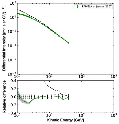
Figure 7.— Differential intensity of CR electrons for PAMELA 2007 datasets. Points represent experimental data, the black dashed line is the GALPROP LIS, and the solid lines are the computed modulated spectra. The bottom panel shows the relative difference between the numerical solution and experimental data.

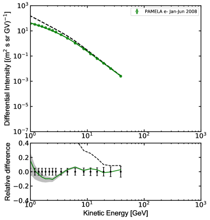
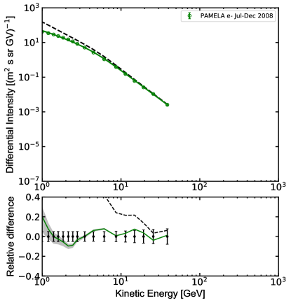
Figure 8.— Differential intensity of CR electrons for PAMELA 2008 datasets. Points represent experimental data, the dashed line is the GALPROP LIS, and the solid line is the computed modulated spectrum. The bottom panel shows the relative difference between the numerical solution and experimental data.

Figure 9.— Differential intensity of CR electrons for PAMELA datasets integrated from January to June 2009. Points represent experimental data, the black dashed line is the GALPROP LIS, and the solid line is the computed modulated spectrum. The bottom panel shows the relative difference between the numerical solution and experimental data.

Table 4Electron LIS

Kinetic energy,	Differential	Kinetic energy,	Differential	Kinetic energy,	Differential	Kinetic energy,	Differential
GeV	intensity	GeV	intensity	GeV	intensity	GeV	intensity
1.000e-03	3.481e+06	3.927e-02	3.225e+04	1.542e+00	6.057e+01	6.482e+01	5.236e-04
1.070e-03	3.710e+06	4.203e-02	2.935e+04	1.651e+00	5.145e+01	6.938e+01	4.167e-04
1.146e-03	3.523e+06	4.499e-02	2.671e+04	1.767e+00	4.370e+01	7.426e+01	3.318e-04
1.226e-03	3.288e+06	4.815e-02	2.431e+04	1.891e+00	3.713e+01	7.949e+01	2.644e-04
1.312e-03	3.056e+06	5.154e-02	2.212e+04	2.024e+00	3.155e+01	8.508e+01	2.108e-04
1.405e-03	2.835e+06	5.517e-02	2.014e+04	2.166e+00	2.681e+01	9.106e+01	1.681e-04
1.504e-03	2.627e+06	5.905e-02	1.834e+04	2.319e+00	2.278e+01	9.747e+01	1.342e-04
1.609e-03	2.431e+06	6.320e-02	1.670e+04	2.482e+00	1.935e+01	1.043e+02	1.071e-04
1.722e-03	2.246e+06	6.764e-02	1.521e+04	2.656e+00	1.642e+01	1.117e+02	8.560e-05
1.844e-03	2.074e+06	7.240e-02	1.386e+04	2.843e+00	1.392e+01	1.195e+02	6.841e-05
1.973e-03	1.912e+06	7.749e-02	1.262e+04	3.043e+00	1.179e+01	1.279e+02	5.470e-05
2.112e-03	1.761e+06	8.295e-02	1.149e+04	3.257e+00	9.962e+00	1.369e+02	4.374e-05
2.261e-03	1.621e+06	8.878e-02	1.046e+04	3.486e+00	8.397e+00	1.465e+02	3.499e-05
2.420e-03	1.490e+06	9.502e-02	9.525e+03	3.732e+00	7.054e+00	1.569e+02	2.800e-05
2.590e-03	1.368e+06	1.017e-01	8.669e+03	3.994e+00	5.904e+00	1.679e+02	2.240e-05
2.772e-03	1.256e+06	1.089e-01	7.887e+03	4.275e+00	4.919e+00	1.797e+02	1.793e-05
2.967e-03	1.151e+06	1.165e-01	7.173e+03	4.576e+00	4.076e+00	1.923e+02	1.435e-05
3.176e-03	1.055e+06	1.247e-01	6.521e+03	4.898e+00	3.358e+00	2.059e+02	1.149e-05
3.399e-03	9.658e+05	1.335e-01	5.926e+03	5.242e+00	2.748e+00	2.203e+02	9.193e-06
3.638e-03	8.835e+05	1.429e-01	5.382e+03	5.611e+00	2.235e+00	2.358e+02	7.358e-06
3.894e-03	8.077e+05	1.529e-01	4.886e+03	6.005e+00	1.806e+00	2.524e+02	5.889e-06
4.168e-03	7.380e+05	1.637e-01	4.433e+03	6.428e+00	1.451e+00	2.702e+02	4.713e-06
4.461e-03	6.739e+05	1.752e-01	4.019e+03	6.880e+00	1.160e+00	2.892e+02	3.772e-06
4.775e-03	6.150e+05	1.875e-01	3.640e+03	7.364e+00	9.239e-01	3.095e+02	3.018e-06
5.111e-03	5.609e+05	2.007e-01	3.295e+03	7.882e+00	7.335e-01	3.313e+02	2.415e-06
5.470e-03	5.114e+05	2.148e-01	2.979e+03	8.436e+00	5.811e-01	3.546e+02	1.932e-06
5.855e-03	4.660e+05	2.299e-01	2.690e+03	9.029e+00	4.598e-01	3.795e+02	1.545e-06
6.267e-03	4.244e+05	2.461e-01	2.426e+03	9.665e+00	3.634e-01	4.062e+02	1.236e-06
6.707e-03	3.864e+05	2.634e-01	2.185e+03	1.034e+01	2.871e-01	4.348e+02	9.887e-07
7.179e-03	3.517e+05	2.819e-01	1.964e+03	1.107e+01	2.268e-01	4.654e+02	7.907e-07
7.684e-03	3.200e+05	3.018e-01	1.762e+03	1.185e+01	1.791e-01	4.981e+02	6.323e-07
8.225e-03	2.910e+05	3.230e-01	1.577e+03	1.268e+01	1.415e-01	5.332e+02	5.056e-07
8.803e-03	2.646e+05	3.457e-01	1.409e+03	1.358e+01	1.118e-01	5.707e+02	4.042e-07
9.422e-03	2.406e+05	3.700e-01	1.255e+03	1.453e+01	8.829e-02	6.108e+02	3.231e-07
1.008e-02	2.186e+05	3.960e-01	1.115e+03	1.555e+01	6.976e-02	6.538e+02	2.583e-07
1.079e-02	1.987e+05	4.239e-01	9.886e+02	1.665e+01	5.512e-02	6.997e+02	2.064e-07
1.155e-02	1.805e+05	4.537e-01	8.739e+02	1.782e+01	4.356e-02	7.489e+02	1.650e-07
1.237e-02	1.640e+05	4.856e-01	7.703e+02	1.907e+01	3.444e-02	8.016e+02	1.318e-07
1.324e-02	1.489e+05	5.198e-01	6.771e+02	2.041e+01	2.722e-02	8.580e+02	1.053e-07
1.417e-02	1.353e+05	5.563e-01	5.934e+02	2.185e+01	2.152e-02	9.184e+02	8.416e-08
1.516e-02	1.229e+05	5.955e-01	5.185e+02	2.339e+01	1.703e-02	9.830e+02	6.724e-08
1.623e-02	1.116e+05	6.374e-01	4.517e+02	2.503e+01	1.347e-02	1.052e+03	5.372e-08
1.737e-02	1.014e+05	6.822e-01	3.923e+02	2.679e+01	1.066e-02	1.126e+03	4.291e-08
1.859e-02	9.206e+04	7.302e-01	3.398e+02	2.867e+01	8.439e-03	1.205e+03	3.427e-08
1.990e-02	8.363e+04	7.815e-01	2.934e+02	3.069e+01	6.680e-03	1.290e+03	2.737e-08
2.130e-02	7.597e+04	8.365e-01	2.527e+02	3.285e+01	5.304e-03	1.381e+03	2.186e-08
2.280e-02	6.903e+04	8.953e-01	2.171e+02	3.516e+01	4.192e-03	1.478e+03	1.746e-08
2.440e-02	6.273e+04	9.583e-01	1.861e+02	3.763e+01	3.316e-03	1.582e+03	1.394e-08
2.612e-02	5.701e+04	1.026e+00	1.592e+02	4.028e+01	2.633e-03	1.693e+03	1.113e-08
2.796e-02	5.182e+04	1.098e+00	1.359e+02	4.311e+01	2.077e-03	1.812e+03	8.888e-09
2.992e-02	4.712e+04	1.175e+00	1.158e+02	4.615e+01	1.649e-03	1.940e+03	7.096e-09
3.203e-02	4.285e+04	1.258e+00	9.861e+01	4.939e+01	1.310e-03	2.076e+03	5.665e-09
3.428e-02	3.897e+04	1.346e+00	8.387e+01	5.287e+01	1.042e-03	2.222e+03	4.522e-09
3.669e-02	3.545e+04	1.441e+00	7.129e+01	5.658e+01	8.282e-04	2.378e+03	3.610e-09

References

- Abdo et al. (2009) Abdo, A. A. et al. 2009, Phys. Rev. Lett., 102, 181101
- Abdollahi et al. (2017) Abdollahi, S. et al. 2017, Phys. Rev. D, 95, 082007
- Accardo et al. (2014) Accardo, L. et al. 2014, Phys. Rev. Lett., 113, 121101
- Ackermann et al. (2012a) Ackermann, M. et al. 2012a, Phys. Rev. Lett., 108, 011103
- Ackermann et al. (2010) —. 2010, Phys. Rev. D, 82, 092004
- Ackermann et al. (2012b) —. 2012b, ApJ, 750, 3
- Adriani et al. (2017) Adriani, O. et al. 2017, Phys. Rev. Lett., 119, 181101
- Adriani et al. (2009) Adriani, O. et al. 2009, Nature, 458, 607
- Adriani et al. (2011) —. 2011, Phys. Rev. Lett., 106, 201101
- Adriani et al. (2015) —. 2015, ApJ, 810, 142
- Adriani et al. (2016) —. 2016, Phys. Rev. Lett., 116, 241105
- Aguilar et al. (2014a) Aguilar, M. et al. 2014a, Phys. Rev. Lett., 113, 221102
- Aguilar et al. (2014b) —. 2014b, Phys. Rev. Lett., 113, 121102
- Aharonian et al. (2009) Aharonian, F. et al. 2009, A&A, 508, 561
- Aharonian et al. (2008) —. 2008, Phys. Rev. Lett., 101, 261104
- Alanko-Huotari et al. (2007) Alanko-Huotari, K., Usoskin, I. G., Mursula, K., & et al. 2007, J. Geophys. Res., 112
- Asaoka et al. (2017) Asaoka, Y. et al. 2017, Astropart. Phys., 91, 1
- Atwood et al. (2009) Atwood, W. B. et al. 2009, ApJ, 697, 1071
- Balogh et al. (2001) Balogh, A., Marsden, R. G., & Smith, E. J. 2001, The heliosphere near solar minimum. The Ulysses perspective
- Barwick et al. (1997) Barwick, S. W. et al. 1997, ApJ, 482, L191
- Barwick et al. (1998) —. 1998, ApJ, 498, 779
- Basini et al. (1995) Basini, G. et al. 1995, 24th Int. Cosmic Ray Conf. (Rome), 3, 1
- Beatty et al. (2004) Beatty, J. J. et al. 2004, Phys. Rev. Lett., 93, 241102
- Bobik et al. (2013) Bobik, P. et al. 2013, Adv. Astron., 2013
- Bobik et al. (2012) —. 2012, ApJ, 745, 132
- Bobik et al. (2009) Bobik, P. et al. 2009, in Astroparticle, Particle and Space Physics, Detectors and Medical Physics Applications: Volume 5. Proceedings of the 11th Conference. Villa Olmo, Como, Italy, 5 – 9 October 2009 (WORLD SCIENTIFIC), 760–764
- Bobik et al. (2016) —. 2016, J. Geophys. Res. (Space Phys.), 121, 3920
- Bobik et al. (2003) Bobik, P., Gervasi, M., Grandi, D., Rancoita, P. G., & Usoskin, I. G. 2003, in Astroparticle, Particle and Space Physics, Detectors and Medical Physics Applications: Volume 2. Proceedings of the 8th Conference Villa Olmo, Como, Italy, 6 – 11 October 2003 (WORLD SCIENTIFIC), 23–28
- Boezio et al. (2000) Boezio, M. et al. 2000, ApJ, 532, 653
- Boschini et al. (2017a) Boschini, M. J. et al. 2017a, ApJ, 840, 115
- Boschini et al. (2017b) Boschini, M. J., Della Torre, S., Gervasi, M., La Vacca, G., & Rancoita, P. G. 2017b, Available online on Adv. Space Res. doi:10.1016/j.asr.2017.04.017
- Buffington et al. (1975) Buffington, A., Orth, C. D., & Smoot, G. F. 1975, ApJ, 199, 669
- Burger & Hattingh (1998) Burger, R. A., & Hattingh, M. 1998, ApJ, 505, 244
- Cummings et al. (2016) Cummings, A. C. et al. 2016, ApJ, 831, 18
- Della Torre et al. (2012) Della Torre, S. et al. 2012, Adv. Space Res., 49, 1587
- Della Torre et al. (2015) Della Torre, S., Gervasi, M., Rancoita, P. G., & et al. 2015, J. High Energy Astrophys., 8, 27
- Dialynas et al. (2017) Dialynas, K., Krimigis, S. M., Mitchell, D. G., Decker, R. B., & Roelof, E. C. 2017, Nature Astron., 1, 0115
- Earl (1961) Earl, J. A. 1961, Phys. Rev. Lett., 6, 125
- Engelbrecht et al. (2017) Engelbrecht, N. E., Strauss, R. D., le Roux, J. A., & Burger, R. A. 2017, ApJ, 841, 107
- Fanselow et al. (1969) Fanselow, J. L., Hartman, R. C., Hildebrad, R. H., & Meyer, P. 1969, ApJ, 158, 771
- Gervasi et al. (1998) Gervasi, M., Rancoita, P., Usoskin, I., & Kovaltsov, G. 1998, Nuclear Physics B Proceedings Supplements, 6th ICATPP Conf., Como 5-9 Oct 1998, 78, 26
- Golden et al. (1994) Golden, R. L. et al. 1994, ApJ, 436, 769
- Golden et al. (1984) Golden, R. L., Mauger, B. G., Badhwar, G. D., Daniel, R. R., Lacy, J. L., Stephens, S. A., & Zipse, J. E. 1984, ApJ, 287, 622
- Golden et al. (1996) Golden, R. L. et al. 1996, ApJ, 457, L103
- Grimani et al. (2002) Grimani, C. et al. 2002, A&A, 392, 287
- Hartman & Pellerin (1976) Hartman, R. C., & Pellerin, C. J. 1976, ApJ, 204, 927
- Jóhannesson et al. (2016) Jóhannesson, G. et al. 2016, ApJ, 824, 16
- Kobayashi et al. (2004) Kobayashi, T., Komori, Y., Yoshida, K., & Nishimura, J. 2004, ApJ, 601, 340
- Lewis & Bridle (2002) Lewis, A., & Bridle, S. 2002, Phys. Rev. D, 66, 103511
- Liu et al. (2012) Liu, J., Yuan, Q., Bi, X.-J., Li, H., & Zhang, X. 2012, Phys. Rev. D, 85, 043507
- Marsden (2001) Marsden, R. G. 2001, The Publications of the Astronomical Society of the Pacific, 113, 129
- Meyer & Vogt (1961) Meyer, P., & Vogt, R. 1961, Phys. Rev. Lett., 6, 193
- Moskalenko et al. (2017) Moskalenko, I. V., Johannesson, G., Orlando, E., Porter, T. A., & Strong, A. W. 2017, Proc. 35th Int. Cosmic Ray Conf. (Busan), PoS(ICRC2017)279
- Moskalenko & Strong (1998) Moskalenko, I. V., & Strong, A. W. 1998, ApJ, 493, 694
- Parker (1965) Parker, E. N. 1965, Planet. Space Sci., 13, 9
- Perko (1987) Perko, J. S. 1987, å, 184, 119
- Porter et al. (2017) Porter, T. A., Jóhannesson, G., & Moskalenko, I. V. 2017, ApJ, 846, 67
- Porter et al. (2008) Porter, T. A., Moskalenko, I. V., Strong, A. W., Orlando, E., & Bouchet, L. 2008, ApJ, 682, 400
- Potgieter & Moraal (1985) Potgieter, M. S., & Moraal, H. 1985, ApJ, 294, 425
- Protheroe (1982) Protheroe, R. J. 1982, ApJ, 254, 391
- Ptuskin et al. (2006) Ptuskin, V. S., Moskalenko, I. V., Jones, F. C., Strong, A. W., & Zirakashvili, V. N. 2006, ApJ, 642, 902
- Rastoin et al. (1996) Rastoin, C. et al. 1996, A&A, 307, 981
- Sanderson et al. (1995) Sanderson, T. R., Marsden, R. G., Wenzel, K.-P., Balogh, A., Forsyth, R. J., & Goldstein, B. E. 1995, Space Science Reviews, 72, 291
- Scherer et al. (2011) Scherer, K., Fichtner, H., Strauss, R. D., Ferreira, S. E. S., Potgieter, M. S., & Fahr, H.-J. 2011, ApJ, 735, 128
- Seo et al. (2014) Seo, E. S. et al. 2014, Adv. Spa. Res., 53, 1451
- Stone et al. (2013) Stone, E. C., Cummings, A. C., McDonald, F. B., Heikkila, B. C., Lal, N., & Webber, W. R. 2013, Science, 341, 150
- Strauss et al. (2011) Strauss, R. D., Potgieter, M. S., Büsching, I., & Kopp, A. 2011, ApJ, 735, 83
- Strong & Moskalenko (1998) Strong, A. W., & Moskalenko, I. V. 1998, ApJ, 509, 212
- Strong et al. (2007) Strong, A. W., Moskalenko, I. V., & Ptuskin, V. S. 2007, Ann. Rev. Nucl. Part. Sci., 57, 285
- Tomassetti et al. (2017) Tomassetti, N., Orcinha, M., Barao, F., & Bertucci, B. 2017, Submitted to ApJ, arXiv: 1707.06916
- Torii et al. (2001) Torii, S. et al. 2001, ApJ, 559, 973
- Vladimirov et al. (2011) Vladimirov, A. E. et al. 2011, Comp. Phys. Comm., 182, 1156