Wigner functions on non-standard symplectic vector spaces

Abstract

We consider the Weyl quantization on a flat non-standard symplectic vector space. We focus mainly on the properties of the Wigner functions defined therein. In particular we show that the sets of Wigner functions on distinct symplectic spaces are different but have non-empty intersections. This extends previous results to arbitrary dimension and arbitrary (constant) symplectic structure. As a by-product we introduce and prove several concepts and results on non-standard symplectic spaces which generalize those on the standard symplectic space, namely the symplectic spectrum, Williamson’s theorem and Narcowich-Wigner spectra. We also show how Wigner functions on non-standard symplectic spaces behave under the action of an arbitrary linear coordinate transformation.

MSC [2000]: Primary 35S99, 35P05; Secondary 35S05, 47A75

Keywords: Weyl quantization; Wigner functions; symplectic spaces; symplectic spectrum; Williamson’s theorem; Narcowich-Wigner spectra

1 Introduction

In this work we return to the research programme initiated in [2, 3]. There we considered the Weyl-Wigner formulation of quantum mechanics based on a canonical deformation of the Heisenberg algebra. More specifically, if $z=(x,p)\in\mathbb{R}^{2n}$ denotes a phase space coordinate of a particle, then the standard classical Poisson bracket is replaced by the following deformation

$$\left\{z_{\alpha},z_{\beta}\right\}=\Omega_{\alpha,\beta},\hskip 28.45274pt1\leq\alpha,\beta\leq 2n,$$ (1)

where $(\Omega_{\alpha,\beta})_{1\leq\alpha,\beta\leq 2n}$ are the entries of the matrix

$${\bf\Omega}=\left(\begin{array}[]{l l}{\bf\Theta}&{\bf I}\\ -{\bf I}&{\bf\Upsilon}\end{array}\right).$$ (2)

Here ${\bf I}$ is the $n\times n$ identity matrix and ${\bf\Theta}=\left(\theta_{ij}\right)_{1\leq i,j\leq n},{\bf\Upsilon}=\left(\eta_{ij}\right)_{1\leq i,j\leq n}$ are real constant skew-symmetric $n\times n$ matrices, which measure the extra noncommutativity in the configuration and momentum spaces, respectively. One assumes in general that this symplectic form does not depart appreciably from the standard one [17]:

$$|\theta_{ij}\eta_{kl}|\ll 1,$$ (3)

for all $i,j,k,l=1,\cdots,n$. Upon quantization, one obtains a deformation of the Heisenberg algebra.

Noncommutative deformations such as this one and others appear in manifold contexts. They may emerge (i) in the various attempts to quantize gravity, such as string theory [72], noncommutative geometry [12, 21, 59] and loop quantum gravity [71]; (ii) as a means to regularize quantum field theories [30, 76]; (iii) as the result of quantizing quantum systems with second class constraints [45, 65, 66]; (iv) in order to stabilize unstable algebras [78], (v) as the low-energy physics of quasicrystals [62], and quite simply (vi) as a model for quantum systems under the influence of an external magnetic field [22]. Regardless of the context and motivation, deforming the Heisenberg algebra in the realm of non-relativistic quantum mechanics [23, 37, 64] has led to many interesting and surprising results such as the thermodynamic stability of black holes [4], regularization of black hole singularities [5, 6, 68], modifications of quantum cosmology scenarios [38, 60], violation of uncertainty principles [8, 11], generation of entanglement due to noncommutativity [7]. These deformations have also been used in the context of the Landau problem [32, 47] and the quantum Hall effect [10].

We shall follow [2, 3] and address quantum mechanics on non-standard symplectic spaces in the framework of the Weyl-Wigner formulation. As explained in [3] there are various aspects of this formulation which make it (in certain circumstances) more appealing than the ordinary formulation in terms of operators acting on a Hilbert space. In the Weyl-Wigner representation one does not have to choose between a position or a momentum representation of a state, as the Wigner function provides a joint distribution of both. It is no surprise that the uncertainty principle and non-locality take their toll on the Wigner function in the form of a lack of positivity [33, 48, 75]. Nevertheless, Wigner functions have positive marginals and permit an evaluation of expectation values of observables with the suggestive formula

$$<\widehat{A}>=\int_{\mathbb{R}^{2n}}a(z)W\rho(z)dz,$$ (4)

where $\widehat{A}$ is a self-adjoint operator, $a$ is its Weyl symbol and $W\rho$ is the Wigner function associated with some density matrix $\rho$. Moreover, the Weyl-Wigner framework is the only phase space formulation which is symplectically invariant [26, 36, 40, 41, 42, 43, 54, 84]. More precisely, if $W\rho(z)$ is a Wigner function and ${\bf S}$ is some symplectic matrix, then $W\rho({\bf S}z)$ is again a Wigner function. This makes it a privileged framework to study the semiclassical limit of quantum mechanics [56, 61, 85]. The symplectic flavour of this approach manifests itself equally in the dynamics of a quantum mechanical system. The time evolution is governed by a quantum counterpart of the Poisson bracket - called Moyal bracket - which is a deformation of the Poisson bracket [9, 34, 35, 53, 63, 77, 82]. From this perspective one sometimes calls this phase space formulation of quantum mechanics deformation quantization.

The Weyl-Wigner formulation is also particularly useful in the context of quantum information with continuous variables [14, 74, 80].

For the quantization of systems with non-standard symplectic spaces, the advantage of the Weyl-Wigner formulation becomes more emphatic. The reason is that the Hilbert space for quantum mechanics on non-standard symplectic spaces is still $L^{2}(\mathbb{R}^{n})$. So in the operator formulation, there is no distinction between states for different symplectic structures. On the other hand, in deformation quantization we proved in [2, 3] that the set of states (Wigner functions) in noncommutative quantum mechanics differs from the set of ordinary Wigner functions. We have used this fact as a criterion for assessing when a transition from noncommutative to ordinary quantum mechanics has taken place [29].

In [3] we considered the set $\mathcal{F}^{C}$ of ordinary Wigner functions, the set $\mathcal{F}^{NC}$ of Wigner functions for the noncommutative symplectic structure (1,2), and the set $\mathcal{L}$ of positive (classical) probability densities. We proved that in dimension $n=2$ any pair of these sets have non-empty intersections and none of them contains the other. The main purpose of the present work is to generalize this result to arbitrary dimension $n$ and to the sets $\mathcal{F}^{\omega_{1}},\mathcal{F}^{\omega_{2}}$ of Wigner functions defined on the symplectic vector spaces $(\mathbb{R}^{2n};\omega_{1}),(\mathbb{R}^{2n};\omega_{2})$ with symplectic forms $\omega_{2}\neq\pm\omega_{1}$. Notice that the sympectic forms are completely arbitrary (not necessarily of the form (2)), albeit constant.

As a byproduct we extend a number of definitions and results concerning ordinary Wigner functions to Wigner functions on arbitrary, nonstandard symplectic spaces. Moreover, as an application of our results, we solve the so-called representability problem in the case of linear coordinate transformations. This terminology was coined in [20, 57] in the context of signal processing for pure states. Here we use the following definition for an arbitrary (pure or mixed) state. A given real and measurable phase-space function $F(z)$ is said to be representable if there exists a density matrix $\rho$ such that $F$ is the Wigner function on some symplectic phase-space associated with $\rho$, i.e. $F=W\rho$. Here we consider linear coordinate transformations of the form

$$W\rho(z)\mapsto(\mathcal{U}_{{\bf M}}W\rho)(z)=|\det M|W\rho({\bf M}z),$$ (5)

with ${\bf M}\in Gl(2n;\mathbb{R})$. We then address the problem of the representability of $\mathcal{U}_{{\bf M}}W\rho$.

Our results may also be potentially interesting for quantum information of continuous variable systems. Indeed, the partial transpose - a linear coordinate transformation which has as sole effect the reversal of the momentum of one subsystem - is neither symplectic nor anti-symplectic [74, 80]. Hence, it maps a Wigner function on the standard symplectic vector space to a Wigner function on a non-standard one. This transformation is used as a criterion to assess whether a state is separable or entangled.

Here is a summary of the main results of this work.

1) We define the notion of Narcowich-Wigner spectrum adapted to an arbitrary symplectic form (Definition 5) and prove its main properties (Theorem 10, Theorem 11).

2) We introduce the symplectic spectrum for an arbitrary symplectic form (Definition 15). We prove a Williamson-type theorem for non-standard symplectic spaces (Theorem 17) and show the usefulness of symplectic spectra for generalized uncertainty principles (Theorem 19). In Theorem 23 we show that we can always find a positive-definite matrix which has distinct symplectic spectra relative to two different symplectic forms. This result is fine-tuned for the smallest symplectic eigenvalue in Theorem 24.

3) We solve the representability problem for linear coordinate transformations in Theorems 25 and 28. In Theorem 25 we prove that $\mathcal{U}_{{\bf M}}W\rho$ is representable for any Wigner function $W\rho$ if and only if ${\bf M}$ is symplectic or antisymplectic. Another new result is Theorem 28, which states that if ${\bf M}$ is neither symplectic nor antisymplectic, then there exists a Wigner function $W\rho$ such that $\mathcal{U}_{{\bf M}}W\rho$ is again a Wigner function and $W\rho^{\prime}$ for which $\mathcal{U}_{{\bf M}}W\rho^{\prime}$ is not a Wigner function.

4) Theorem 27 is one of the main results of this work and it shows that in the phase-space formulation different quantizations (i.e. on different symplectic spaces) yield different sets of states. However, there are always positive distributions and states that are common to different quantizations. These results are valid in arbitrary dimension and for arbitrary flat sympletic vector spaces.

Notation

We denote by $\mathbb{P}_{k\times k}(\mathbb{K})$ the convex cone of real $(\mathbb{K}=\mathbb{R})$ (or complex $(\mathbb{K}=\mathbb{C})$) symmetric (hermitean) positive (semi-definite) $k\times k$ matrices, and we write $\mathbb{P}_{k\times k}^{\times}(\mathbb{K})$ if they are positive-definite. The set of real skew-symmetric $k\times k$ matrices is $A(k;\mathbb{R})$. The space of Schwartz test functions is denoted by $\mathcal{S}(\mathbb{R}^{n})$ and its dual $\mathcal{S}^{\prime}(\mathbb{R}^{n})$ are the tempered distributions. Latin indices $i,j,k,\cdots$, take values in the set $\left\{1,2,\cdots,n\right\}$, whereas Greek indices $\alpha,\beta,\gamma,\cdots$ are phase space indices which take values in $\left\{1,2,\cdots,2n\right\}$. The inner product in $L^{2}(\mathbb{R}^{n})$ is given by

$$<\psi|\phi>=\int_{\mathbb{R}^{n}}\overline{\psi(x)}\phi(x)dx.$$ (6)

We may at times write $<\psi|\phi>_{L^{2}(\mathbb{R}^{n})}$ and $||\psi||_{L^{2}(\mathbb{R}^{n})}$ for the corresponding norm if we want to emphasize that the functions are defined on the $n$-dimensional Euclidean space $\mathbb{R}^{n}$.

The Fourier-Plancherel transform for a function $f\in L^{1}(\mathbb{R}^{n})\cap L^{2}(\mathbb{R}^{n})$ is defined by

$$(\mathcal{F}f)(\omega)=\int_{\mathbb{R}^{n}}f(x)e^{-ix\cdot\omega}dx$$ (7)

and its inverse is

$$(\mathcal{F}^{-1}f)(x)=\frac{1}{(2\pi)^{n}}\int_{\mathbb{R}^{n}}f(\omega)e^{ix\cdot\omega}d\omega.$$ (8)

In this work, we choose units such that Planck’s constant is $h=2\pi\hbar=2\pi$.

2 Symplectic vector spaces

Let $V$ be some real $2n$-dimensional vector space. A symplectic form on $V$ is a skew-symmetric non-degenerate bilinear form, that is a map $\omega:V\times V\to\mathbb{R}$ such that

$$\omega(\alpha x+\beta y,z)=\alpha\omega(x,z)+\beta\omega(y,z),\hskip 28.45274pt\omega(x,y)=-\omega(y,x),$$ (9)

for all $x,y,z\in V$ and $\alpha,\beta\in\mathbb{R}$, and

$$\omega(x,y)=0,\mbox{ for all }y\in V$$ (10)

if and only if $x=0$.

The symplectic group $Sp(V;\omega)$ is the group of linear automorphisms $\phi:V\to V$ such that

$$\omega\left(\phi(z),\phi(z^{\prime})\right)=\omega(z,z^{\prime}),$$ (11)

for all $z,z^{\prime}\in V$. An automorphism $\phi$ is said to be anti-symplectic if

$$\omega\left(\phi(z),\phi(z^{\prime})\right)=-\omega(z,z^{\prime}),$$ (12)

for all $z,z^{\prime}\in V$. The archetypal symplectic vector space is $V=\mathbb{R}^{2n}$ endowed with the so-called standard symplectic form. As usual we write $z=(x,p)\in V=\mathbb{R}^{n}\times(\mathbb{R}^{n})^{\ast}\simeq\mathbb{R}^{2n}$, where $x\in\mathbb{R}^{n}$ is interpreted as the particle’s position and $p\in(\mathbb{R}^{n})^{\ast}$ as the particle’s momentum belonging to the cotangent bundle. The standard symplectic form reads

$$\sigma(z,z^{\prime})=z\cdot{\bf J^{-1}}z^{\prime}=p\cdot x^{\prime}-x\cdot p^{\prime},$$ (13)

where $z=(x,p)$, $z^{\prime}=(x^{\prime},p^{\prime})$ and ${\bf J}=-{\bf J^{-1}}=-{\bf J^{T}}$ is the $2n\times 2n$ standard symplectic matrix

$${\bf J}=\left(\begin{array}[]{c c}{\bf 0}&{\bf I}\\ -{\bf I}&{\bf 0}\end{array}\right).$$ (14)

The symplectic group $Sp(\mathbb{R}^{2n};\sigma)\equiv Sp(n;\sigma)$ is then the set of matrices ${\bf P}$ such that

$${\bf P}{\bf J}{\bf P^{T}}={\bf J}.$$ (15)

We remark that if ${\bf P}\in Sp(n;\sigma)$, then also ${\bf P^{-1}},{\bf P^{T}}\in Sp(n;\sigma)$.

A matrix ${\bf A}$ is $\sigma$-anti-symplectic [26] if

$${\bf A}{\bf J}{\bf A^{T}}=-{\bf J}.$$ (16)

All $\sigma$-anti-symplectic matrices ${\bf A}$ can be written as

$${\bf A}={\bf R}{\bf P},$$ (17)

where ${\bf P}\in Sp(n;\sigma)$ and

$${\bf R}=\left(\begin{array}[]{c c}{\bf I}&{\bf 0}\\ {\bf 0}&-{\bf I}\end{array}\right).$$ (18)

Thus a $\sigma$-anti-symplectic transformation is a $\sigma$-symplectic transformation followed by a reflection of the particle’s momentum.

More generally, for any other symplectic form on $\mathbb{R}^{2n}$, there exists a real skew-symmetric matrix ${\bf\Omega}\in Gl(2n)$ such that

$$\omega(z,z^{\prime})=z\cdot{\bf\Omega^{-1}}z^{\prime},\hskip 28.45274ptz,z^{\prime}\in\mathbb{R}^{2n}.$$ (19)

A well known theorem in symplectic geometry [16, 40] states that all symplectic vector spaces of equal dimension are symplectomorphic. In other words, if $(V,\omega)$ and $(V^{\prime},\omega^{\prime})$ have the same dimension, then there exists a linear isomorphism $\phi:V\to V^{\prime}$ such that

$$\phi^{\ast}\omega^{\prime}=\omega.$$ (20)

Here $\phi^{\ast}$ denotes the pull-back of $\phi$. In particular, $(\mathbb{R}^{2n},\sigma)$ is symplectomorphic with $(\mathbb{R}^{2n},\omega)$ for any symplectic form (19). So if $\phi:(\mathbb{R}^{2n},\sigma)\to(\mathbb{R}^{2n},\omega)$ is given by

$$\phi(z)={\bf S}z,$$ (21)

for some ${\bf S}\in Gl(2n)$, then we have from (20) that

$$\phi^{\ast}\omega=\sigma\Leftrightarrow\omega({\bf S}z,{\bf S}z^{\prime})=\sigma(z,z^{\prime}),$$ (22)

for all $z,z^{\prime}\in\mathbb{R}^{2n}$. And thus

$${\bf\Omega}={\bf S}{\bf J}{\bf S^{T}}.$$ (23)

The matrix ${\bf S}$ in (23) is not unique. Indeed, we have

Lemma 1

Suppose that ${\bf S}$ is a solution of (23). Then ${\bf S^{\prime}}$ is also a solution if and only if ${\bf S^{\prime-1}S},{\bf S^{-1}S^{\prime}}\in Sp(n;\sigma)$.

Proof. We have ${\bf\Omega}={\bf S}{\bf J}{\bf S^{T}}={\bf S^{\prime}}{\bf J}{\bf S^{\prime T}}$ if and only if ${\bf S^{\prime-1}S}{\bf J}({\bf S^{\prime-1}S})^{T}={\bf S^{-1}S^{\prime}}{\bf J}({\bf S^{-1}S^{\prime}})^{T}={\bf J}$.   

We denote by $\mathcal{D}(n;\omega)$ the set of all real $2n\times 2n$ matrices satisfying (23) and call them Darboux matrices. The corresponding symplectic automorphism (21) is called a Darboux map.

A matrix ${\bf M}$ is $\omega$-symplectic if

$${\bf M}{\bf\Omega}{\bf M^{T}}={\bf\Omega},$$ (24)

and it is $\omega$-anti-symplectic if

$${\bf M}{\bf\Omega}{\bf M^{T}}=-{\bf\Omega}.$$ (25)

Any $\omega$-symplectic (resp. $\omega$-anti-symplectic) matrix ${\bf M}$ is of the form

$${\bf M}={\bf S}{\bf P}{\bf S^{-1}},$$ (26)

where ${\bf S}\in\mathcal{D}(n;\omega)$ and ${\bf P}$ is a $\sigma$-symplectic (resp. $\sigma$-anti-symplectic) matrix.

For future reference we consider the following Proposition.

Proposition 2

Let $\eta$ be an arbitrary symplectic form on $\mathbb{R}^{2n}$ such that

$$|\eta(z,z^{\prime})|\leq|\sigma(z,z^{\prime})|,$$ (27)

for all $z,z^{\prime}\in\mathbb{R}^{2n}$. Then, there exists a constant $0<|a|\leq 1$ such that

$$\eta=a\sigma.$$ (28)

Proof. Let $\eta(z,z^{\prime})=z^{T}{\bf\Sigma^{-1}}z^{\prime}$ for $z,z^{\prime}\in\mathbb{R}^{2n}$ and ${\bf\Sigma}\in Gl(2n;\mathbb{R})$. Let $\left\{\delta_{\alpha}\right\}_{1\leq\alpha\leq 2n}$ denote the canonical basis of $\mathbb{R}^{2n}$. If we set $z=\delta_{\alpha}$ and $z^{\prime}=\delta_{\beta}$ in (27), we obtain:

$$|\Sigma_{\alpha\beta}^{-1}|\leq|J_{\alpha\beta}|,$$ (29)

for all $1\leq\alpha,\beta\leq 2n$. So $\Sigma_{\alpha\beta}^{-1}=0$, whenever $J_{\alpha\beta}=0$. And so ${\bf\Sigma^{-1}}$ must be of the form

$${\bf\Sigma^{-1}}=\left(\begin{array}[]{c c}{\bf 0}&{\bf D}\\ -{\bf D}&{\bf 0}\end{array}\right),$$ (30)

where ${\bf D}=diag(\mu_{1},\cdots,\mu_{n})$. Next set $z=\delta_{i}-\delta_{j}$ and $z^{\prime}=\delta_{n+i}+\delta_{n+j}$, for $1\leq i<j\leq n$. A simple calculation shows that

$$\sigma(z,z^{\prime})=0,\hskip 28.45274pt\eta(z,z^{\prime})=\mu_{i}-\mu_{j}.$$ (31)

But from (27) it follows that $\mu_{i}=\mu_{j}$ for all $1\leq i<j\leq n$. And so there exists $a\neq 0$ such that (28) holds. But again from (27), we must have $0<|a|\leq 1$.   

3 Weyl Quantization

3.1 Weyl quantization on $(\mathbb{R}^{2n};\sigma)$

One of the basic ingredients for the quantization of a classical system defined on the standard symplectic vector space $(\mathbb{R}^{2n};\sigma)$ is the Heisenberg-Weyl algebra:

$$\left[\widehat{Z}_{\alpha},\widehat{Z}_{\beta}\right]=iJ_{\alpha\beta}\widehat{I},\hskip 14.22636pt\left[\widehat{Z}_{\alpha},\widehat{I}\right]=0,\hskip 28.45274pt\alpha,\beta=1,\cdots,2n,$$ (32)

where $\widehat{Z}=(\widehat{q},\widehat{p})$ are the quantum-mechanical counterparts of the classical phase-space variables $z=(x,p)$ and $\widehat{I}$ is the identity operator. Their action on functions in their (densely defined) domains in $L^{2}(\mathbb{R}^{n})$ is given by

$$(\widehat{I}\psi)(x)=\psi(x),\hskip 28.45274pt(\widehat{q}_{i}\psi)(x)=x_{i}\psi(x),\hskip 28.45274pt(\widehat{p}_{j}\psi)(x)=-i\partial_{j}\psi(x),$$ (33)

for $i,j=1,\cdots,n$. These operators are not bounded, which prevents the construction of a $C^{*}$-algebra of observables. A familiar way to circumvent this is to consider the alternative algebra of Heisenberg-Weyl displacement operators:

$$\widehat{D^{\sigma}}(\xi)=e^{i\sigma(\xi,\widehat{Z})}.$$ (34)

The action of $\widehat{D^{\sigma}}(\xi)$ on $\psi\in\mathcal{S}(\mathbb{R}^{n})$ is given by the explicit formula

$$\widehat{D^{\sigma}}(\xi)\psi(x)=e^{ip_{0}\cdot x-\frac{i}{2}p_{0}\cdot x_{0}}\psi(x-x_{0}),$$ (35)

for $\xi=(x_{0},p_{0})$. This extends to a unitary operator from $L^{2}(\mathbb{R}^{n})$ to $L^{2}(\mathbb{R}^{n})$ and to a continuous operator from $\mathcal{S}^{\prime}(\mathbb{R}^{n})$ to $\mathcal{S}^{\prime}(\mathbb{R}^{n})$.

Their commutation relations are easily established from (35) or, heuristically, from (32,34) using the Baker-Campbell-Hausdorff formula:

$$\widehat{D^{\sigma}}(\xi)\widehat{D^{\sigma}}(\zeta)=e^{\frac{i}{2}\sigma(\xi,\zeta)}\widehat{D^{\sigma}}(\xi+\zeta)=e^{i\sigma(\xi,\zeta)}\widehat{D^{\sigma}}(\zeta)\widehat{D^{\sigma}}(\xi),$$ (36)

for $\xi,\zeta\in\mathbb{R}^{2n}$. Operators of the form

$$\widehat{U}^{\sigma}(\xi,\tau)=e^{i\tau}\widehat{D^{\sigma}}(\xi)$$ (37)

constitute an irreducible unitary representation of the Heisenberg group $\mathbb{H}(n)$ of elements $(\xi,\tau)\in\mathbb{R}^{2n}\times\mathbb{R}$ with group multiplication

$$(\xi,\tau)\cdot(\xi^{\prime},\tau^{\prime})=\left(\xi+\xi^{\prime},\tau+\tau^{\prime}+\frac{1}{2}\sigma(\xi,\xi^{\prime})\right).$$ (38)

This is called the Schrödinger representation and, according to the Stone-von Neumann theorem [70], it is in fact the only unitary irreducible representation of $\mathbb{H}(n)$ on $L^{2}(\mathbb{R}^{n})$ up to rescalings of Planck’s constant.

Given a tempered distribution $a^{\sigma}\in\mathcal{S}^{\prime}(\mathbb{R}^{2n})$ [44, 46], the Weyl operator with symbol $a^{\sigma}$ is the Bochner integral [31, 36, 40, 69, 84]

$$\widehat{A}:=\left(\frac{1}{2\pi}\right)^{n}\int_{\mathbb{R}^{2n}}\mathcal{F}_{\sigma}a^{\sigma}(z)\widehat{D^{\sigma}}(z)dz.$$ (39)

Here $\mathcal{F}_{\sigma}a$ denotes the symplectic Fourier transform

$$\mathcal{F}_{\sigma}a(z):=\left(\frac{1}{2\pi}\right)^{n}\int_{\mathbb{R}^{2n}}e^{-i\sigma(z,z^{\prime})}a(z^{\prime})dz^{\prime}.$$ (40)

We note that $\mathcal{F}_{\sigma}$ in (40) extends into an involutive automorphism $\mathcal{S}^{\prime}(\mathbb{R}^{n})\rightarrow\mathcal{S}^{\prime}(\mathbb{R}^{n})$.

The Weyl correspondence, written $\widehat{A}\overset{\mathrm{Weyl}}{\longleftrightarrow}a^{\sigma}$ or $a^{\sigma}\overset{\mathrm{Weyl}}{\longleftrightarrow}\widehat{A}$ between a symbol $a^{\sigma}\in\mathcal{S}^{\prime}(\mathbb{R}^{2n})$ and the associated Weyl operator $\widehat{A}$ is a one-to-one map from $\mathcal{S}^{\prime}(\mathbb{R}^{2n})$ onto the space $\mathcal{L}\left(\mathcal{S}(\mathbb{R}^{n}),\mathcal{S}^{\prime}(\mathbb{R}^{n})\right)$ of bounded linear operators $\mathcal{S}(\mathbb{R}^{n})\to\mathcal{S}^{\prime}(\mathbb{R}^{n})$. This can be proven using Schwartz’s kernel Theorem and the fact that the Weyl symbol $a^{\sigma}$ of the operator $\widehat{A}$ is related with the distributional kernel $K_{a}$ of that operator by a partial Fourier transform [13, 40, 84]:

$$a^{\sigma}(x,p)=\int_{\mathbb{R}^{n}}e^{-iy\cdot p}K_{a}\left(x+\frac{y}{2},x-\frac{y}{2}\right)dy,$$ (41)

where $K_{a}\in\mathcal{S}^{\prime}(\mathbb{R}^{2n})$ and the Fourier transform is defined in the usual distributional sense.

Conversely, by the Fourier inversion theorem, the kernel $K_{a}$ can be expressed in terms of the symbol $a^{\sigma}$:

$$K_{a}(x,y)=\left(\frac{1}{2\pi}\right)^{n}\int_{\mathbb{R}^{n}}e^{ip\cdot(x-y)}a^{\sigma}\left(\frac{x+y}{2},p\right)dp.$$ (42)

A Weyl operator is formally self-adjoint if and only if its symbol $a^{\sigma}$ is real.

Now, let $\psi\in L^{2}(\mathbb{R}^{n})$ and define the rank-one operator $\widehat{\rho_{\psi}}$

$$\widehat{\rho_{\psi}}\phi=<\psi|\phi>\psi,$$ (43)

for all $\phi\in L^{2}(\mathbb{R}^{n})$. This is a Hilbert-Schmidt operator with kernel:

$$K_{\rho_{\psi}}(x,y)=\psi(x)\overline{\psi(y)}.$$ (44)

The corresponding Weyl symbol is (cf.(41)):

$$\rho^{\sigma}_{\psi}(x,p)=\int_{\mathbb{R}^{n}}e^{-iy\cdot p}\psi\left(x+\frac{y}{2}\right)\overline{\psi\left(x-\frac{y}{2}\right)}dy$$ (45)

which is proportional to the celebrated Wigner function [81]:

$$W^{\sigma}\psi(x,p):=\left(\frac{1}{2\pi}\right)^{n}\rho_{\psi}^{\sigma}(x,p).$$ (46)

The multiplicative constant $(2\pi)^{-n}$ is included to ensure the correct normalization

$$\int_{\mathbb{R}^{2n}}W^{\sigma}\psi(z)dz=1,$$ (47)

whenever $||\psi||_{L^{2}}=1$.

The operator $\widehat{\rho_{\psi}}$ is the density matrix of the pure state $\psi$. Density matrices provide a unified formulation of pure and mixed states, playing a key role in many different contexts, notably semi-classical limit, decoherence, etc [39]. Let then $\left\{p_{\alpha}\right\}_{\alpha}$ be some probability distribution

$$0\leq p_{\alpha}\leq 1,\hskip 28.45274pt\sum_{\alpha}p_{\alpha}=1,$$ (48)

and $\left\{\widehat{\rho}_{\alpha}\right\}_{\alpha}$ a collection of pure state density matrices associated with normalized states $\psi_{\alpha}\in L^{2}(\mathbb{R}^{n})$. The statistical mixture

$$\widehat{\rho}=\sum_{\alpha}p_{\alpha}\widehat{\rho}_{\alpha}$$ (49)

is called the density matrix of a mixed state. One needs some caution in interpreting eq.(49). The usual statement that the system is in state $\widehat{\rho}_{\alpha}$ with probability $p_{\alpha}$ is not very rigorous, because there are (in general infinitely) many different decompositions of a density matrix of the form (49).

An useful way to tell pure states from mixed states is to compute the so-called purity of the state. Moyal’s identity [63] states that if $\psi,\phi\in L^{2}(\mathbb{R}^{n})$, then $W^{\sigma}\psi,W^{\sigma}\phi\in L^{2}(\mathbb{R}^{2n})$ and that:

$$<W^{\sigma}\psi|W^{\sigma}\phi>_{L^{2}(\mathbb{R}^{2n})}=\frac{1}{(2\pi)^{n}}\left|<\psi|\phi>_{L^{2}(\mathbb{R}^{n})}\right|^{2}.$$ (50)

In particular:

$$(2\pi)^{n}||W^{\sigma}\psi||_{L^{2}(\mathbb{R}^{2n})}^{2}=||\psi||_{L^{2}(\mathbb{R}^{n})}^{4}=1.$$ (51)

On the other hand, if we have a mixed state $W^{\sigma}\rho$, then:

$$(2\pi)^{n}||W^{\sigma}\rho||_{L^{2}(\mathbb{R}^{2n})}^{2}<1.$$ (52)

The purity of a state $W^{\sigma}\rho$ is defined by

$$0<\mathcal{P}\left[W^{\sigma}\rho\right]=(2\pi)^{n}||W^{\sigma}\rho||_{L^{2}(\mathbb{R}^{2n})}^{2}\leq 1,$$ (53)

and we have

$$\begin{array}[]{l l}\mathcal{P}\left[W^{\sigma}\rho\right]=1&\mbox{if }W^{\sigma}\rho\mbox{ is a pure state}\\ &\\ \mathcal{P}\left[W^{\sigma}\rho\right]<1&\mbox{if }W^{\sigma}\rho\mbox{ is a mixed state}\end{array}$$ (54)

It is a well known fact from the theory of compact operators [70] that an operator $\widehat{\rho}$ can be written as in (48,49) if and only if it is a positive and trace-class operator with unit trace. If $\rho(x,y)$ is the corresponding kernel then the associated Wigner function is

$$\begin{array}[]{c}W^{\sigma}\rho(x,p)=\left(\frac{1}{2\pi}\right)^{n}\int_{\mathbb{R}^{n}}e^{-iy\cdot p}\rho\left(x+\frac{y}{2},x-\frac{y}{2}\right)dy=\\ \\ =\sum_{\alpha}p_{\alpha}W^{\sigma}\psi_{\alpha}(x,p),\end{array}$$ (55)

with uniform convergence. If $\widehat{A}\overset{\mathrm{Weyl}}{\longleftrightarrow}a^{\sigma}$ is some self-adjoint operator such that $\widehat{A}\widehat{\rho}$ is trace-class then the expectation value of $\widehat{A}$ in the state $\widehat{\rho}$ can be evaluated according to the following remarkable formula.

$$<\widehat{A}>_{\widehat{\rho}}=Tr(\widehat{A}\widehat{\rho})=\int_{\mathbb{R}^{2n}}a^{\sigma}(z)W^{\sigma}\rho(z)dz.$$ (56)

Because of this formula and of the fact that Wigner functions have positive marginal distributions, one is tempted to interpret them as joint position and momentum probability densities. However, this is precluded by their lack of positivity as stated in Hudson’s Theorem [33, 48, 75].

3.2 Weyl quantization on $(\mathbb{R}^{2n};\omega)$

Alternatively, one may choose to quantize the system on a non-standard symplectic vector space $(\mathbb{R}^{2n};\omega)$ with symplectic form $\omega$ given by (19) [2, 3, 18, 19, 24, 25].

Upon quantization, the Heisenberg-Weyl algebra (32) is replaced by the algebra

$$\left[\widehat{\Xi}_{\alpha},\widehat{\Xi}_{\beta}\right]=i\Omega_{\alpha\beta}\widehat{I},\hskip 14.22636pt\left[\widehat{\Xi}_{\alpha},\widehat{I}\right]=0,\hskip 28.45274pt\alpha,\beta=1,\cdots,2n.$$ (57)

In the sequel, we shall assume that

$$\det{\bf\Omega}=1,\hskip 28.45274pt\det{\bf S}=\pm 1,$$ (58)

for all ${\bf S}\in\mathcal{D}(n;\omega)$. This is because different values of the determinant of ${\Omega}$ simply amount to a rescaling of the variables $\left\{\widehat{\Xi}_{\alpha}\right\}_{1\leq\alpha\leq 2n}$ (or, equivalently of a rescaling of Planck’s constant).

Upon exponentiation of (57), we obtain the non-standard Heisenberg-Weyl displacement operators:

$$\widehat{D}^{\omega}(\xi)=e^{i\omega(\xi,\widehat{\Xi})},$$ (59)

satisfying the commutation relations

$$\widehat{D}^{\omega}(\xi)\widehat{D}^{\omega}(\zeta)=e^{\frac{i}{2}\omega(\xi,\zeta)}\widehat{D}^{\omega}(\xi+\zeta)=e^{i\omega(\xi,\zeta)}\widehat{D}^{\omega}(\zeta)\widehat{D}^{\omega}(\xi).$$ (60)

As before, the elements of the form

$$\widehat{U}^{\omega}(\xi,\tau)=e^{i\tau}\widehat{D}^{\omega}(\xi),$$ (61)

constitute a unitary irreducible representation of the modified Heisenberg group $\mathbb{H}^{\omega}(n)$ with multiplication

$$(\xi,\tau)\cdot(\xi^{\prime},\tau^{\prime})=\left(\xi+\xi^{\prime},\tau+\tau^{\prime}+\frac{1}{2}\omega(\xi,\xi^{\prime})\right).$$ (62)

Notice that if ${\bf S}\in\mathcal{D}(n;\omega)$ and $\widehat{Z}$ obey the Heisenberg-Weyl algebra (32), then

$$\widehat{\Xi}={\bf S}\widehat{Z}$$ (63)

satisfy (57). Consequently, we may write

$$\widehat{D}^{\omega}(\xi)=e^{i\omega(\xi,\widehat{\Xi})}=e^{i\omega(\xi,{\bf S}\widehat{Z})}=e^{i\sigma({\bf S^{-1}}\xi,\widehat{Z})}=\widehat{D}^{\sigma}({\bf S^{-1}}\xi).$$ (64)

From this relation and eq.(36), one easily proves the commutation relations (60).

Also, if we perform the transformation $\xi\mapsto z={\bf S}\xi$ with ${\bf S}\in\mathcal{D}(n;\omega)$ in (39) and substitute (64), we obtain:

$$\widehat{A}=\left(\frac{1}{2\pi}\right)^{n}\int_{\mathbb{R}^{2n}}\mathcal{F}_{\sigma}a^{\sigma}({\bf S^{-1}}\xi)\widehat{D}^{\omega}(\xi)d\xi$$ (65)

Next notice that

$$\begin{array}[]{c}\mathcal{F}_{\sigma}a({\bf S^{-1}}\xi)=\left(\frac{1}{2\pi}\right)^{n}\int_{\mathbb{R}^{2n}}e^{-i\sigma({\bf S^{-1}}\xi,z)}a(z)dz=\\ \\ =\left(\frac{1}{2\pi}\right)^{n}\int_{\mathbb{R}^{2n}}e^{-i\omega(\xi,{\bf S}z)}a(z)dz=\\ \\ =\left(\frac{1}{2\pi}\right)^{n}\int_{\mathbb{R}^{2n}}e^{-i\omega(\xi,\xi^{\prime})}a({\bf S^{-1}}\xi^{\prime})d\xi^{\prime}.\end{array}$$ (66)

This then suggests the following definition of the $\omega$-symplectic Fourier transform [25]:

$$\mathcal{F}_{\omega}a(\xi):=\frac{1}{(2\pi)^{n}}\int_{\mathbb{R}^{2n}}e^{-i\omega(\xi,\xi^{\prime})}a(\xi^{\prime})d\xi^{\prime},$$ (67)

for any $a\in\mathcal{S}^{\prime}(\mathbb{R}^{2n})$. With this choice of normalization $\mathcal{F}_{\omega}$ is involutive $\mathcal{F}_{\omega}\mathcal{F}_{\omega}a=a$.

Also we define the $\omega$-Weyl symbol of the operator $\widehat{A}$:

$$a^{\omega}(\xi):=a^{\sigma}({\bf S^{-1}}\xi).$$ (68)

Altogether, from (65-68), we obtain:

$$\widehat{A}=\frac{1}{(2\pi)^{n}}\int_{\mathbb{R}^{2n}}\mathcal{F}_{\omega}a^{\omega}(\xi)\widehat{D}^{\omega}(\xi)d\xi,$$ (69)

which defines the correspondence principle between an operator $\widehat{A}$ and its $\omega$-Weyl symbol $a^{\omega}$. From eq.(46,56) it follows that

$$\begin{array}[]{c}<\widehat{A}>_{\widehat{\rho}}=\frac{1}{(2\pi)^{n}}\int_{\mathbb{R}^{2n}}a^{\sigma}(z)\rho^{\sigma}(z)dz=\\ \\ =\frac{1}{(2\pi)^{n}}\int_{\mathbb{R}^{2n}}a^{\sigma}({\bf S^{-1}}\xi)\rho^{\sigma}({\bf S^{-1}}\xi)d\xi=\\ \\ =\frac{1}{(2\pi)^{n}}\int_{\mathbb{R}^{2n}}a^{\omega}(\xi)\rho^{\omega}(\xi)d\xi=\\ \\ =\int_{\mathbb{R}^{2n}}a^{\omega}(\xi)W^{\omega}\rho(\xi)d\xi,\end{array}$$ (70)

where

$$W^{\omega}\rho(\xi)=W^{\sigma}\rho({\bf S^{-1}}\xi),$$ (71)

is the $\omega$-Wigner function associated with the density matrix $\widehat{\rho}$ [2, 3, 18, 19, 51].

Regarding the purity of the states on the non-standard symplectic space $(\mathbb{R}^{2n};\omega)$ we have:

$$\begin{array}[]{c}\mathcal{P}\left[W^{\omega}\rho\right]=(2\pi)^{n}\int_{\mathbb{R}^{2n}}|W^{\omega}\rho(\xi)|^{2}d\xi=(2\pi)^{n}\int_{\mathbb{R}^{2n}}|W^{\sigma}\rho({\bf S^{-1}}\xi)|^{2}d\xi=\\ \\ =(2\pi)^{n}\int_{\mathbb{R}^{2n}}|W^{\sigma}\rho(z)|^{2}dz=\mathcal{P}\left[W^{\sigma}\rho\right]\end{array}$$ (72)

And thus, we have as before

$$\begin{array}[]{l l}\mathcal{P}\left[W^{\omega}\rho\right]=1&\mbox{if }W^{\omega}\rho\mbox{ is a pure state}\\ &\\ \mathcal{P}\left[W^{\omega}\rho\right]<1&\mbox{if }W^{\omega}\rho\mbox{ is a mixed state}\end{array}$$ (73)

We conclude that the main structures of standard quantum mechanics extend trivially to the non-standard symplectic case. However, there are also significative differences concerning the properties of states. We will address these issues in the next section.

Remark 3

At this point it is worth going back to the partial transpose transformation mentioned in the introduction in relation to the separability problem for systems with continuous variables.

Suppose that a system is constituted of two subsystems - Alice and Bob - with $n^{A}$ and $n^{B}$ degrees of freedom $(n=n^{A}+n^{B})$. Their coordinates are $z^{A}=(x^{A},p^{A})$ and $z^{B}=(x^{B},p^{B})$. We write the collective coordinate $z=(x^{A},x^{B},p^{A},p^{B})$. The partial transpose transformation reverses Bob’s momentum [74, 80]:

$$z\mapsto{\bf P}z=\left(\begin{array}[]{c c c r}{\bf I}&{\bf 0}&{\bf 0}&{\bf 0}\\ {\bf 0}&{\bf I}&{\bf 0}&{\bf 0}\\ {\bf 0}&{\bf 0}&{\bf I}&{\bf 0}\\ {\bf 0}&{\bf 0}&{\bf 0}&-{\bf I}\end{array}\right)~{}\left(\begin{array}[]{c}x^{A}\\ x^{B}\\ p^{A}\\ p^{B}\end{array}\right)=\left(\begin{array}[]{c}x^{A}\\ x^{B}\\ p^{A}\\ -p^{B}\end{array}\right)$$ (74)

A straightforward computation reveals that the transformation ${\bf P}={\bf P^{-1}}$ is neither $\sigma$-symplectic nor $\sigma$-anti-symplectic. Consequently, in general, $W^{\sigma}\psi({\bf P^{-1}}z)$ is not a $\sigma$-Wigner function. Rather, one can think of ${\bf P}$ as a Darboux map for the symplectic form

$$\omega(z,z^{\prime})=z^{T}{\bf\Omega^{-1}}z^{\prime},$$ (75)

with

$${\bf\Omega}={\bf P}{\bf J}{\bf P^{T}}.$$ (76)

And hence, $W^{\omega}\psi(z)=W^{\sigma}\psi({\bf P^{-1}}z)$ is a Wigner function on the non-standard symplectic space with symplectic form (75,76).

4 States in phase-space

In this section we shall always consider real, normalized and square-integrable functions defined on the phase-space $\mathbb{R}^{2n}$. A difficult problem consists in assessing whether such a function $f$ qualifies as a $\omega$-Wigner function for some symplectic form $\omega$. In other words, how can one tell if $f$ is the $\omega$-Wigner function of some density matrix $\widehat{\rho}$?

It is well known that the answer lies in the following positivity condition [27, 55]. A real and normalized function $f\in L^{2}(\mathbb{R}^{2n})$ is a $\sigma$-Wigner function if and only if

$$\int_{\mathbb{R}^{2n}}f(z)W^{\sigma}\psi(z)dz\geq 0,$$ (77)

for all $\psi\in L^{2}(\mathbb{R}^{n})$. On the other hand, $f$ is a $\omega$-Wigner function if and only if there exist a $\sigma$-Wigner function $f^{\sigma}$ and a matrix ${\bf S}\in\mathcal{D}(n;\omega)$ such that $f(\xi)=f^{\sigma}({\bf S}^{-1}\xi)$. That happens if and only if

$$\begin{array}[]{c}\int_{\mathbb{R}^{2n}}f(\xi)W^{\omega}\psi(\xi)d\xi=\int_{\mathbb{R}^{2n}}f^{\sigma}({\bf S}^{-1}\xi)W^{\sigma}\psi({\bf S}^{-1}\xi)d\xi=\\ \\ =\int_{\mathbb{R}^{2n}}f^{\sigma}(z)W^{\sigma}\psi(z)dz\geq 0,\end{array}$$ (78)

for all $\psi\in L^{2}(\mathbb{R}^{n})$.

The positivity conditions (77,78) are somewhat tautological, as they require the knowledge of the entire set of $\sigma$- or $\omega$-Wigner functions of pure states. There are an alternative set of conditions which are more in the spirit of measure theory and Bochner’s Theorem. They were derived by Kastler [52], and Loupias and Miracle-Sole [58] using the machinery of $C^{\ast}$-algebras and were later synthesized by Narcowich [67] in the framework of the so-called Narcowich-Wigner (NW) spectrum. This proved to be a very powerful tool to address convolutions of functions defined on the phase-space as we shall shortly see.

Here is a brief summary of the remainder of this section. In the next subsection, we define the NW spectrum of a function for a given symplectic structure and show how it provides a condition of positivity alternative to (77) or (78). In Theorem 10, we show how the NW spectrum behaves under the convolution. In Theorem 11 we gather the main properties of NW spectra. In subsection 4.2 we consider the uncertainty principle in the Robertson-Schrödinger form and the associated concept of symplectic spectrum for a given symplectic form $\omega$. The main results of this subsection are the Williamson Theorem for a non-standard symplectic form (Theorem 17) and Theorem 24 which shows that one can find positive-definite matrices with lowest symplectic eigenvalues with respect to two different sympletic strucutes as far apart as one wishes. All these results culminate in Theorem 27 of section 4.3, where we show how the sets of positive (classical) measures and the sets of Wigner functions for two distinct symplectic structures relate to each other. Finally, as an application, we prove in Theorem 28 how a Wigner function behaves under an arbitrary linear coordinate transformation.

4.1 Narcowich-Wigner spectra

Definition 4

Let ${\bf\Sigma}\in A(2n;\mathbb{R})$ and $\alpha\in\mathbb{R}$. A complex-valued, continuous function $f$ on $\mathbb{R}^{2n}$ that has the property that the matrix $\left[\left[M_{jk}\right]\right]$ with entries

$$M_{jk}=f(a_{j}-a_{k})e^{\frac{i\alpha}{2}a_{k}\cdot{\bf\Sigma}a_{j}}$$ (79)

is a positive matrix on $\mathbb{C}^{N}$ for each $N\in\mathbb{N}$ and all $a_{1},a_{2},\cdots,a_{N}\in\mathbb{R}^{2n}$ is called a function of the $(\alpha,{\bf\Sigma})$-positive type. If $\alpha=0$, then we shall simply say that $f$ is of the $0$-positive type.

A function may be of the $(\alpha,{\bf\Sigma})$-positive type for various values of $\alpha$ and these can be assembled in a set.

Definition 5

The ${\bf\Sigma}$-Narcowich-Wigner spectrum of a complex-valued, continuous function $f$ on $\mathbb{R}^{2n}$ is the set:

$$\mathcal{W}^{{\bf\Sigma}}(f):=\left\{\alpha\in\mathbb{R}:~{}f\mbox{ is of the $(\alpha,{\bf\Sigma})$-positive type}\right\}.$$ (80)

More generally the Narcowich-Wigner spectrum of $f$ is the set:

$$\mathcal{W}(f):=\left\{(\alpha,{\bf\Sigma})\in\mathbb{R}\times A(2n;\mathbb{R}):~{}f\mbox{ is of the $(\alpha,{\bf\Sigma})$-positive type}\right\}.$$ (81)

For each $\alpha\in\mathbb{R}$ and ${\bf\Sigma}\in A(2n;\mathbb{R})$ the set of all functions of $(\alpha,{\bf\Sigma})$-positive type is a convex cone.

Before we proceed let us briefly recall Bochner’s Theorem.

Theorem 6

(Bochner) The set of Fourier transforms of finite, positive measures on $\mathbb{R}^{k}$ $(k\in\mathbb{N})$ is exactly the cone of functions of $0$-positive type.

The KLM (Kastler, Loupias, Miracle-Sole) conditions are a twisted generalization of Bochner’s theorem.

Theorem 7

(Kastler, Loupias, Miracle-Sole) Let $f$ be a real function on the phase-space $\mathbb{R}^{2n}$. Then $f$ is a $\sigma$-Wigner function if and only if its Fourier transform $\mathcal{F}(f)$ satisfies the $\sigma$-KLM conditions:

(i) $\mathcal{F}(f)(0)=1$;

(ii) $\mathcal{F}(f)$ is of the $(1,{\bf J})$-positive type.

The first condition ensures the normalization of $f$, while the second one is equivalent to the positivity condition (77). In terms of the Narcowich-Wigner spectrum, condition (ii) means

$$1\in\mathcal{W}^{{\bf J}}(\mathcal{F}(f)).$$ (82)

On the other hand, if $f$ is everywhere non-negative, then according to Bochner’s theorem

$$0\in\mathcal{W}^{{\bf\Sigma}}(\mathcal{F}(f)),$$ (83)

for all ${\bf\Sigma}\in A(2n;\mathbb{R})$.

We now generalize the KLM conditions (Theorem 7) for an arbitrary symplectic form $\omega$.

Theorem 8

Let $f$ be a real function on the phase-space $\mathbb{R}^{2n}$. Then $f$ is a $\omega$-Wigner function if and only if its Fourier transform $\mathcal{F}(f)$ satisfies the $\omega$-KLM conditions:

(i) $\mathcal{F}(f)(0)=1$;

(ii) $\mathcal{F}(f)$ is of the $(1,{\bf\Omega})$-positive type.

Proof. As usual $f$ is a $\omega$-Wigner function if and only if there exists a $\sigma$-Wigner function $f^{\sigma}$ and a matrix ${\bf S}\in\mathcal{D}(n;\omega)$ such that $f(z)=f^{\sigma}({\bf S}^{-1}z)$. After a simple calculation, we conclude that $\mathcal{F}(f)(a)=\mathcal{F}(f^{\sigma})({\bf S}^{T}a)$. Consequently:

$$\begin{array}[]{c}\mathcal{F}(f)(a_{j}-a_{k})e^{\frac{i\alpha}{2}a_{k}\cdot{\bf\Omega}a_{j}}=\mathcal{F}(f^{\sigma})({\bf S}^{T}(a_{j}-a_{k}))e^{\frac{i\alpha}{2}a_{k}\cdot{\bf\Omega}a_{j}}=\\ \\ =\mathcal{F}(f^{\sigma})(b_{j}-b_{k})e^{\frac{i\alpha}{2}b_{k}\cdot{\bf S}^{-1}{\bf\Omega}({\bf S}^{T})^{-1}b_{j}}=\mathcal{F}(f^{\sigma})(b_{j}-b_{k})e^{\frac{i\alpha}{2}b_{k}\cdot{\bf J}b_{j}}\end{array}$$ (84)

with $b_{j}={\bf S}^{T}a_{j}$ for $j=1,\cdots,N$. We conclude that $\mathcal{W}^{{\bf\Omega}}(\mathcal{F}(f))=\mathcal{W}^{{\bf J}}(\mathcal{F}(f^{\sigma}))$ and the result follows.   

Remark 9

It follows from the proof that $(\alpha,{\bf\Omega})\in\mathcal{W}(\mathcal{F}(f))$ if and only if $(\alpha,{\bf J})\in\mathcal{W}(\mathcal{F}(f^{\sigma}))$.

Before we proceed, let us recapitulate the concept of Hamard-Schur (HS) product. Let ${\bf A}=\left[\left[A_{ij}\right]\right],{\bf B}=\left[\left[B_{ij}\right]\right]\in M(k\times n;\mathbb{C})$. Then the HS product is the map $\diamondsuit:M(k\times n;\mathbb{C})\times M(k\times n;\mathbb{C})\to M(k\times n;\mathbb{C})$

$${\bf A}\diamondsuit{\bf B}=\left[\left[A_{ij}B_{ij}\right]\right].$$ (85)

According to Schur’s Theorem, the HS product has the property of being a closed operation in the convex cone $\mathbb{P}_{k\times k}(\mathbb{C})$ of positive $k\times k$ matrices, i.e.:

$$\diamondsuit:\mathbb{P}_{k\times k}(\mathbb{C})\times\mathbb{P}_{k\times k}(\mathbb{C})\to\mathbb{P}_{k\times k}(\mathbb{C}).$$ (86)

Theorem 10

Let $f,g\in L^{1}(\mathbb{R}^{2n})$ be real-valued functions on $\mathbb{R}^{2n}$, such that $\mathcal{F}(f),\mathcal{F}(g)$ are of the $(\alpha,{\bf\Sigma})$ and of the $(\beta,{\bf\Upsilon})$-positive type, respectively, and $\det(\alpha{\bf\Sigma}+\beta{\bf\Upsilon})\neq 0$. Moreover, define $\gamma:=\left(\det(\alpha{\bf\Sigma}+\beta{\bf\Upsilon})\right)^{\frac{1}{2n}}$ to be a real $(2n)$-th root of that determinant (this is always possible since real antisymmetric matrices have non-negative determinants; they are equal to the square of a polynomial of its entries - the Pfaffian). Then the Fourier transform of the convolution $f\star g$ is of the $\left(\gamma,\frac{\alpha}{\gamma}{\bf\Sigma}+\frac{\beta}{\gamma}{\bf\Upsilon}\right)$-positive type. For later convenience we write:

$$(\alpha,{\bf\Sigma})\oplus(\beta,{\bf\Upsilon})=\left(\gamma,\frac{\alpha}{\gamma}{\bf\Sigma}+\frac{\beta}{\gamma}{\bf\Upsilon}\right).$$ (87)

Proof. Since $f,g\in L^{1}(\mathbb{R}^{2n})$, the Fourier transform of the convolution amounts to the pointwise product $\mathcal{F}(f\star g)=\mathcal{F}(f)\cdot\mathcal{F}(g)$. Thus:

$$\begin{array}[]{c}\mathcal{F}(f\star g)(a_{j}-a_{k})e^{\frac{i\gamma}{2}\left(\frac{\alpha}{\gamma}a_{k}\cdot{\bf\Sigma}+\frac{\beta}{\gamma}{\bf\Upsilon}\right)a_{j}}=\\ \\ =\left(\mathcal{F}(f)(a_{j}-a_{k})e^{\frac{i\alpha}{2}a_{k}\cdot{\bf\Sigma}a_{j}}\right)\left(\mathcal{F}(g)(a_{j}-a_{k})e^{\frac{i\beta}{2}a_{k}\cdot{\bf\Upsilon}a_{j}}\right).\end{array}$$ (88)

The last expression is the $(jk)$-th component of the HS product of two positive matrices and the result follows.   

Henceforth, we shall use the notation $\mathcal{G}_{{\bf A}}$ to represent the phase-space Gaussian with covariance matrix ${\bf A}$:

$$\mathcal{G}_{{\bf A}}(z)=\frac{1}{(2\pi)^{n}\sqrt{\det{\bf A}}}\exp\left(-\frac{1}{2}z\cdot{\bf A^{-1}}z\right).$$ (89)

We are tacitly assuming that the expectation values $<\widehat{Z}_{i}>$ are all equal to zero, something which can easily be achieved by a phase-space translation.

For later convenience we assemble the following properties of Narcowich-Wigner spectra (see [15, 28, 67] for the standard symplectic case):

Theorem 11

Let $\Omega\in A(2n;\mathbb{R})$, $\mathcal{W}^{{\bf\Omega}}(\mathcal{F}(f))$ denote ${\Omega}$-Narcowich-Wigner spectrum of $\mathcal{F}(f)$ for some function $f\in L^{2}(\mathbb{R}^{2n})$ with continuous Fourier transform. Then the following properties hold.

1. If $\mathcal{F}(f)$ is of $(\alpha,{\bf\Omega})$-positive type for some $\alpha\in\mathbb{R}$ and some ${\bf\Omega}\in A(2n;\mathbb{R})$, then $f$ is a real function.

2. $\mathcal{W}^{{\bf\Omega}}(\mathcal{F}(f^{\vee}))=\mathcal{W}^{{\bf\Omega}}(\mathcal{F}(f))$, where $f^{\vee}(z)=f(-z)$.

3. $\alpha\in\mathcal{W}^{{\bf\Omega}}(\mathcal{F}(f))$ if and only if $-\alpha\in\mathcal{W}^{{\bf\Omega}}(\mathcal{F}(f))$.

4. Let $f_{\lambda}(z)=|\lambda|^{2n}f(\lambda z)$ for $\lambda\in\mathbb{R}\backslash\left\{0\right\}$. Then $\mathcal{W}^{{\bf\Omega}}(\mathcal{F}(f_{\lambda}))=\frac{1}{\lambda^{2}}\mathcal{W}^{{\bf\Omega}}(\mathcal{F}(f))$.

5. Let $\det{\bf\Omega}=1$ and $\omega(z,z^{\prime})=z\cdot{\bf\Omega^{-1}}z^{\prime}$ is the associated symplectic form. For ${\bf M}\in Sl(2n;\mathbb{R})$ define $f_{{\bf M}}(z)=f({\bf M}z)$. Then if ${\bf M}$ is $\omega$-symplectic or $\omega$-anti symplectic, we have $\mathcal{W}^{{\bf\Omega}}(\mathcal{F}(f_{{\bf M}}))=\mathcal{W}^{{\bf\Omega}}(\mathcal{F}(f))$.

6. Let $\psi\in L^{2}(\mathbb{R}^{n})$ be some pure state and $\omega(z,z^{\prime})=z^{\prime}\cdot{\bf\Omega^{-1}}z$ an arbitrary symplectic form. If $\psi$ is a Gaussian function, then $\mathcal{W}^{{\bf\Omega}}(\mathcal{F}(W^{\omega}\psi))=\left[-1,1\right]$. Otherwise $\mathcal{W}^{{\bf\Omega}}(\mathcal{F}(W^{\omega}\psi))=\left\{-1,1\right\}$.

Proof.

1. Suppose that $(\alpha,{\bf\Omega})\in\mathcal{W}(\mathcal{F}(f))$. Then the matrices with entries $M_{jk}=\mathcal{F}(f)(a_{j}-a_{k})e^{\frac{i\alpha}{2}a_{k}\cdot{\bf\Omega}a_{j}}$ are positive in $\mathbb{C}^{N}$. For $N=2$, we have that

   $$\left(\begin{array}[]{c c}\mathcal{F}(f)(0)&\mathcal{F}(f)(a_{1}-a_{2})e^{\frac{i\alpha}{2}a_{2}\cdot{\bf\Omega}a_{1}}\\ &\\ \mathcal{F}(f)(a_{2}-a_{1})e^{\frac{i\alpha}{2}a_{1}\cdot{\bf\Omega}a_{2}}&\mathcal{F}(f)(0)\end{array}\right)$$

   is positive. In particular it has to be self-adjoint, and setting $\omega:=a_{1}-a_{2}$, we obtain:

   $$\overline{\mathcal{F}(f)(\omega)}=\mathcal{F}(f)(-\omega)$$

   for all $\omega\in\mathbb{R}^{2n}$, where we used the continuity of $\mathcal{F}(f)$. This is equivalent to $f$ being a real function.

2. A simple calculation shows that $\mathcal{F}(f^{\vee})=\left[\mathcal{F}(f)\right]^{\vee}$. It follows that

   $$\mathcal{F}(f^{\vee})(a_{j}-a_{k})e^{\frac{i\alpha}{2}a_{k}\cdot{\bf\Omega}a_{j}}=\mathcal{F}(f)(a_{k}-a_{j})e^{\frac{i\alpha}{2}a_{k}\cdot{\bf\Omega}a_{j}}=\mathcal{F}(f)(b_{j}-b_{k})e^{\frac{i\alpha}{2}b_{k}\cdot{\bf\Omega}b_{j}}$$

   where $b_{j}=-a_{j}$, etc. If follows that $(\alpha,{\bf\Omega})\in\mathcal{W}^{{\bf\Omega}}(\mathcal{F}(f^{\vee}))$ if and only if $(\alpha,{\bf\Omega})\in\mathcal{W}^{{\bf\Omega}}(\mathcal{F}(f))$.

3. We have

   $$\begin{array}[]{c}\mathcal{F}(f)(a_{j}-a_{k})e^{-\frac{i\alpha}{2}a_{k}\cdot{\bf\Omega}a_{j}}=\left[\mathcal{F}(f)\right]^{\vee}(a_{k}-a_{j})e^{\frac{i\alpha}{2}a_{j}\cdot{\bf\Omega}a_{k}}=\\ \\ =\mathcal{F}(f^{\vee})(a_{k}-a_{j})e^{\frac{i\alpha}{2}a_{j}\cdot{\bf\Omega}a_{k}}\end{array}$$

   and the result follows from 2.

4. Since $\mathcal{F}f_{\lambda}(z)=\mathcal{F}f\left(\frac{z}{\lambda}\right)$, we have that

   $$\mathcal{F}f_{\lambda}(a_{j}-a_{k})e^{-\frac{i\alpha}{2}a_{k}\cdot{\bf\Omega}a_{j}}=\mathcal{F}f\left(\frac{a_{j}}{\lambda}-\frac{a_{k}}{\lambda}\right)e^{-\frac{i\alpha}{2}a_{k}\cdot{\bf\Omega}a_{j}}=\mathcal{F}f(b_{j}-b_{k})e^{-\frac{i\alpha\lambda^{2}}{2}b_{k}\cdot{\bf\Omega}b_{j}},$$

   with $a_{j}=\lambda b_{j}$. We conclude that $\alpha\in\mathcal{W}^{{\bf\Omega}}(\mathcal{F}(f_{\lambda}))$ if and only if $\alpha\lambda^{2}\in\mathcal{W}^{{\bf\Omega}}(\mathcal{F}(f))$.

5. We have that ${\bf M}{\bf\Omega}{\bf M^{T}}=\epsilon{\bf\Omega}$ with $\epsilon=+1$ (resp. $\epsilon=-1$) if ${\bf M}$ is $\omega$-symplectic (resp. $\omega$-anti symplectic).

   On the other hand, we have $\mathcal{F}f_{{\bf M}}(z)=\mathcal{F}f(({\bf M^{-1}})^{T}z)$. Thus

   $$\begin{array}[]{c}\mathcal{F}f_{{\bf M}}(a_{j}-a_{k})e^{-\frac{i\alpha}{2}a_{k}\cdot{\bf\Omega}a_{j}}=\mathcal{F}f\left(({\bf M^{-1}})^{T}a_{j}-({\bf M^{-1}})^{T}a_{k}\right)e^{-\frac{i\alpha}{2}a_{k}\cdot{\bf\Omega}a_{j}}=\\ \\ =\mathcal{F}f(b_{j}-b_{k})e^{-\frac{i\alpha}{2}b_{k}\cdot{\bf M}{\bf\Omega}{\bf M^{T}}b_{j}}=\mathcal{F}f(b_{j}-b_{k})e^{-\frac{i\alpha\epsilon}{2}b_{k}\cdot{\bf\Omega}b_{j}},\end{array}$$

   where $a_{j}={\bf M^{T}}b_{j}$. We conclude that $\alpha\in\mathcal{W}^{{\bf\Omega}}(\mathcal{F}(f_{{\bf M}})$ if and only if $\epsilon\alpha\in\mathcal{W}^{{\bf\Omega}}(\mathcal{F}(f))$. The rest is a consequence of 3.

6. We proved in [28] that $\mathcal{W}^{{\bf\sigma}}(\mathcal{F}(W^{\sigma}\psi))=\left[-1,1\right]$ if $\psi$ is a Gaussian function, and $\mathcal{W}^{{\bf\sigma}}(\mathcal{F}(W^{\sigma}\psi))=\left\{-1,1\right\}$ otherwise. The rest is a consequence of Remark 9.

 

4.2 Uncertainty principle and symplectic spectra

Consider again the Gaussian measure (89). It is well known that this is the Wigner function associated with some density matrix if and only if [67]:

$${\bf A}+\frac{i}{2}{\bf J}\geq 0,$$ (90)

that is ${\bf A}+\frac{i}{2}{\bf J}$ is a positive matrix in $\mathbb{C}^{2n}$. This matrix inequality is known in the literature as the Robertson-Schrödinger uncertainty principle (RSUP). It is stronger than the more familiar Heisenberg inequality (see below), as it also accounts for the position-momentum correlations. It also has the advantage of being invariant under linear symplectic transformations. Indeed, if $W^{\sigma}\rho(z)$ is the Wigner function of some density matrix $\widehat{\rho}$ and ${\bf P}\in Sp(n;\sigma)$, then $W^{\sigma}\rho({\bf P}z)$ is the Wigner function $W^{\sigma}\rho_{{\bf P}}$ of some other density matrix $\widehat{\rho}_{{\bf P}}$, related to $\widehat{\rho}$ by a metaplectic transformation [54, 73, 79]. Accordingly, if ${\bf A_{\rho}}$ and ${\bf A_{\rho_{P}}}$ are the corresponding covariance matrices, then the two are related by the following transformation:

$${\bf A_{\rho}}={\bf P}{\bf A_{\rho_{P}}}{\bf P^{T}},$$ (91)

where we used the fact that $\det{\bf P}=1$ for ${\bf P}\in Sp(n;\sigma)$. Thus:

$${\bf A_{\rho}}+\frac{i}{2}{\bf J}\geq 0\Leftrightarrow{\bf A_{\rho_{P}}}+\frac{i}{2}{\bf P^{-1}}{\bf J}{\bf\left(P^{-1}\right)^{T}}\geq 0\Leftrightarrow{\bf A_{\rho_{P}}}+\frac{i}{2}{\bf J}\geq 0,$$ (92)

since ${\bf P^{-1}}\in Sp(n;\sigma)$.

To establish whether a state satisfies the RSUP (90), one computes the eigenvalues of the matrix ${\bf A}+\frac{i}{2}{\bf J}$ and verifies if they are all greater or equal to zero. Alternatively, we may verify the RSUP by resorting to the symplectic eigenvalues of ${\bf A}$ and Williamson’s Theorem.

First notice that if ${\bf A}\in\mathbb{P}^{\times}_{2n\times 2n}(\mathbb{R})$, then the matrix ${\bf A}{\bf J^{-1}}$ has the same eigenvalues as ${\bf A^{1/2}}{\bf J^{-1}}{\bf A^{1/2}}$ [83]. So the eigenvalues of ${\bf A}{\bf J^{-1}}$ come in pairs $\pm i\lambda_{\sigma,j}({\bf A})$, where $\lambda_{\sigma,j}({\bf A})>0$, $j=1,\cdots,n$.

Definition 12

Let $\lambda_{\sigma,j}({\bf A})$, $j=1,\cdots,n$ denote the moduli of the eigenvalues of ${\bf A}{\bf J^{-1}}$ written as an increasing sequence

$$0<\lambda_{\sigma,1}({\bf A})\leq\lambda_{\sigma,2}({\bf A})\leq\cdots\leq\lambda_{\sigma,n}({\bf A}).$$ (93)

They are called the $\sigma$-Williamson invariants or $\sigma$-symplectic eigenvalues of ${\bf A}$, and the $n$-tuple

$$Spec_{\sigma}({\bf A}):=\left(\lambda_{\sigma,1}({\bf A}),\lambda_{\sigma,2}({\bf A}),\cdots,\lambda_{\sigma,n}({\bf A})\right)$$ (94)

is called the $\sigma$-symplectic spectrum of ${\bf A}$.

The invariance of the $\sigma$-symplectic spectrum of ${\bf A}$ under the transformation ${\bf A}\mapsto{\bf A^{\prime}}={\bf P}{\bf A}{\bf P^{T}}$ with ${\bf P}\in Sp(n;\sigma)$ is easily established. Indeed suppose that $\lambda\in Spec_{\sigma}({\bf A})$. Then

$$\begin{array}[]{c}0=\det({\bf A}{\bf J^{-1}}\pm i\lambda{\bf I})=\det({\bf P^{-1}}{\bf A^{\prime}}{\bf P^{-1T}}{\bf J^{-1}}\pm i\lambda{\bf I})=\\ \\ =\det({\bf P^{-1}}{\bf A^{\prime}}{\bf J^{-1}}{\bf P}\pm i\lambda{\bf I})=\det({\bf A^{\prime}}{\bf J^{-1}}\pm i\lambda{\bf I}),\end{array}$$ (95)

where we used ${\bf J}{\bf P^{T}}={\bf P^{-1}}{\bf J}$. Thus $Spec_{\sigma}({\bf A^{\prime}})=Spec_{\sigma}({\bf A})$.

The following theorem is due to Williamson [83]:

Theorem 13

(Williamson) Let $A\in\mathbb{P}^{\times}_{2n\times 2n}(\mathbb{R})$. There exists a symplectic matrix ${\bf P}\in Sp(n;\sigma)$ such that

$${\bf P}{\bf A}{\bf P^{T}}=diag\left(\lambda_{\sigma,1}({\bf A}),\cdots,\lambda_{\sigma,n}({\bf A}),\lambda_{\sigma,1}({\bf A}),\cdots,\lambda_{\sigma,n}({\bf A})\right),$$ (96)

where $\lambda_{\sigma,j}({\bf A})$, $j=1,\cdots,n$ are the $\sigma$-Williamson invariants of ${\bf A}$.

We are now in a position to reexpress the RSUP in terms of the $\sigma$-symplectic spectrum. Let ${\bf A}$ be the covariance matrix of some Wigner function $W^{\sigma}\rho(z)$ and let ${\bf D}$ denote the diagonal matrix appearing in (96). We thus have

$${\bf A}+\frac{i}{2}{\bf J}\geq 0\Leftrightarrow{\bf D}+\frac{i}{2}{\bf P}{\bf J}{\bf P^{T}}\geq 0\Leftrightarrow{\bf D}+\frac{i}{2}{\bf J}\geq 0.$$ (97)

The eigenvalues of the last matrix are easily computed. They are equal to $\lambda_{\sigma,j}({\bf A})\pm\frac{1}{2}$, $j=1,\cdots,n$. Thus the last inequality in (97) holds if and only if [67]

$$\lambda_{\sigma,1}({\bf A})\geq\frac{1}{2}.$$ (98)

Let now $W^{\sigma}\rho(z)$ be some Wigner function with covariance matrix ${\bf A}$. Let ${\bf P}\in Sp(n;\sigma)$ be the symplectic matrix diagonalizing ${\bf A}$ as in (96). As we argued before, $W^{\sigma}\rho({\bf P^{-1}}z)$ corresponds to another Wigner function $W^{\sigma}\rho_{{\bf P}}(z)$ with covariance matrix ${\bf P}{\bf A}{\bf P^{T}}={\bf D}$ (cf.(91,96)). This means that since the covariance matrix of $W^{\sigma}\rho_{{\bf P}}(z)$ is diagonal, we have

$$<\widehat{q}_{j}^{2}>_{\rho_{{\bf P}}}=<\widehat{p}_{j}^{2}>_{\rho_{{\bf P}}}=\lambda_{\sigma,j}({\bf A}),\hskip 28.45274ptj=1,\cdots,n$$ (99)

Thus

$$<\widehat{q}_{j}^{2}>_{\rho_{{\bf P}}}<\widehat{p}_{j}^{2}>_{\rho_{{\bf P}}}=\left(\lambda_{\sigma,j}({\bf A})\right)^{2}\geq\frac{1}{4},\hskip 28.45274ptj=1,\cdots,n$$ (100)

which is the Heisenberg uncertainty principle. Consequently, the lowest value of $\frac{1}{2}$ for each $\sigma$-symplectic eigenvalue (cf.(98)), corresponds to a minimal uncertainty in some direction in the phase-space. Thus the extremal situation, where

$$\lambda_{\sigma,1}({\bf A})=\lambda_{\sigma,2}({\bf A})=\cdots=\lambda_{\sigma,n}({\bf A})=\frac{1}{2},$$ (101)

(which is equivalent to $2{\bf A}\in Sp(n;\sigma)$) can only be achieved by a Gaussian pure state. This is known in the literature as Littlejohn’s Theorem [1, 56].

For future reference we state and prove the following proposition.

Proposition 14

Let $e,f\in\mathbb{R}^{2n}$ be such that $\sigma(f,e)\neq 0$. Then there exists a matrix ${\bf A}\in\mathbb{P}^{\times}_{2n\times 2n}(\mathbb{R})$ such that $u=e+if$ is an eigenvector of $i{\bf A}{\bf J^{-1}}$ with eigenvalue equal to $\lambda_{\sigma,1}({\bf A})$ (if $\sigma(f,e)>0$) or $-\lambda_{\sigma,1}({\bf A})$ (if $\sigma(f,e)<0$), where $\lambda_{\sigma,1}({\bf A})$ is the smallest $\sigma$-Williamson invariant of ${\bf A}$.

Proof. Suppose that $\lambda_{1}:=\sigma(f,e)>0$. Set $f^{\prime}=\frac{f}{\sqrt{\lambda_{1}}}$ and $e^{\prime}=\frac{e}{\sqrt{\lambda_{1}}}$. It follows that $\sigma(f^{\prime},e^{\prime})=1$. A well known theorem in symplectic geometry [16, 40] states that we can find a symplectic basis $\left\{e_{i}^{\prime},f_{j}^{\prime}\right\}_{1\leq i,j\leq n}$ such that $e_{1}^{\prime}=e^{\prime}$ and $f_{1}^{\prime}=f^{\prime}$. Next choose an arbitrary set of positive numbers $\lambda_{2},\lambda_{3},\cdots,\lambda_{n}$ such that $\lambda_{1}\leq\lambda_{2}\leq\cdots\leq\lambda_{n}$, and define

$$e_{i}=\sqrt{\lambda_{i}}e_{i}^{\prime},\hskip 28.45274ptf_{j}=\sqrt{\lambda_{j}}f_{j}^{\prime},\hskip 28.45274pt1\leq i,j\leq n.$$ (102)

Now define $v_{i}=e_{i}$, and $v_{i+n}=f_{i}$ (and similarly $v_{i}^{\prime}=e_{i}^{\prime}$, and $v_{i+n}^{\prime}=f_{i}^{\prime}$), and $\lambda_{i+n}=\lambda_{i}$ for $i=1,\cdots,n$. We can now rewrite (102) in a more compact manner:

$$v_{\alpha}=\sqrt{\lambda_{\alpha}}v_{\alpha}^{\prime},\hskip 28.45274pt1\leq\alpha\leq 2n.$$ (103)

Since $\left\{v_{\alpha}^{\prime}\right\}_{1\leq\alpha\leq 2n}$ is a symplectic basis, we have:

$$\sigma(v_{\alpha},v_{\beta})=\sqrt{\lambda_{\alpha}\lambda_{\beta}}\sigma(v_{\alpha}^{\prime},v_{\beta}^{\prime})=\sqrt{\lambda_{\alpha}\lambda_{\beta}}J_{\beta\alpha}=\lambda_{\alpha}J_{\beta\alpha},$$ (104)

where we used the fact that $\lambda_{i+n}=\lambda_{i}$, for $i=1,2,\cdots,n$. In general the basis $\left\{v_{\alpha}\right\}_{1\leq\alpha\leq 2n}$ is not orthonormal. However, there exists a matrix ${\bf A}\in\mathbb{P}^{\times}_{2n\times 2n}(\mathbb{R})$ such that

$$v_{\alpha}^{T}{\bf A^{-1}}v_{\beta}=\delta_{\alpha\beta},\hskip 28.45274pt1\leq\alpha,\beta\leq 2n.$$ (105)

The matrix ${\bf A}$ defines an inner product in $\mathbb{C}^{2n}$:

$$<z,z^{\prime}>_{{\bf A}}:=\overline{z}\cdot{\bf A^{-1}}z^{\prime},\hskip 28.45274ptz,z^{\prime}\in\mathbb{C}^{2n}.$$ (106)

We conclude the proof by showing that $(\lambda_{1},\lambda_{2},\cdots,\lambda_{n})$ is the symplectic spectrum of ${\bf A}$ and that ${\bf A}{\bf J^{-1}}(e+if)=-i\lambda_{1}(e+if)$.

Let $T:\mathbb{R}^{2n}\to\mathbb{R}^{2n}$ be the linear transformation $T(v)={\bf AJ^{-1}}v$, with matrix representation ${\bf AJ^{-1}}$ in the canonical basis. Then

$$<v_{\alpha},T\left(v_{\beta}\right)>_{{\bf A}}=\sigma(v_{\alpha},v_{\beta})=\lambda_{\alpha}J_{\beta\alpha}.$$ (107)

So the matrix representation ${\bf T}$ of $T$ with respect to the basis $\left\{v_{\alpha}\right\}_{1\leq\alpha\leq 2n}$ is

$${\bf T}=\left(\begin{array}[]{c c}{\bf 0}&-{\bf\Lambda}\\ {\bf\Lambda}&{\bf 0}\end{array}\right),$$ (108)

where ${\bf\Lambda}=diag(\lambda_{1},\cdots,\lambda_{n})$. The eigenvalues of ${\bf T}$ (and hence of $T$) are easily computed. They are: $\left\{\pm i\lambda_{j}\right\}_{j=1,\cdots,n}$ and the associated eigenvectors of ${\bf AJ^{-1}}$ are:

$${\bf AJ^{-1}}(e_{j}\pm if_{j})=\mp i\lambda_{j}(e_{j}\pm if_{j}),\hskip 28.45274ptj=1,\cdots,n.$$ (109)

In particular ${\bf AJ^{-1}}(e+if)=-i\lambda_{1}(e+if)$.

If $\sigma(f,e)<0$, then by following an identical procedure, we would obtain: ${\bf AJ^{-1}}(e+if)=i\lambda_{1}(e+if)$.   

Now we turn to the non-standard symplectic space $(\mathbb{R}^{2n};\omega)$. Suppose that $W^{\omega}\rho(z)$ is some $\omega$-Wigner function and let ${\bf S}\in\mathcal{D}(n;\omega)$ denote an arbitrary Darboux matrix. According to (71)

$$W^{\sigma}\rho(z):=W^{\omega}\rho({\bf S}z)$$ (110)

is a $\sigma$-Wigner function. Hence it has to comply with RSUP. Let ${\bf A}^{\sigma}$ and ${\bf A}^{\omega}$ denote the covariance matrices of $W^{\sigma}\rho$ and $W^{\omega}\rho$, respectively. We thus have

$${\bf A}^{\omega}={\bf S}{\bf A}^{\sigma}{\bf S^{T}}.$$ (111)

Consequently,

$${\bf A}^{\sigma}+\frac{i}{2}{\bf J}\geq 0\Leftrightarrow{\bf A}^{\omega}+\frac{i}{2}{\bf S}{\bf J}{\bf S^{T}}\geq 0\Leftrightarrow{\bf A}^{\omega}+\frac{i}{2}{\bf\Omega}\geq 0.$$ (112)

The last inequality is valid irrespective of whatever Darboux matrix ${\bf S}$ we use. We shall call this inequality the $\omega$-RSUP.

Next let ${\bf A}\in\mathbb{P}^{\times}_{2n\times 2n}(\mathbb{R})$, and consider the eigenvalues of the matrix ${\bf A}{\bf\Omega^{-1}}$. As in the standard case ${\bf AJ^{-1}}$, these come in pairs $\pm i\lambda_{\omega,j}({\bf A})$, $\lambda_{\omega,j}({\bf A})>0$, $j=1,\cdots,n$.

Definition 15

The moduli of the eigenvalues of ${\bf A}{\bf\Omega^{-1}}$ written as an increasing sequence $0<\lambda_{\omega,1}({\bf A})\leq\lambda_{\omega,2}({\bf A})\leq\cdots\leq\lambda_{\omega,n}({\bf A})$ will be called the $\omega$-Williamson invariants or the $\omega$-symplectic eigenvalues of ${\bf A}$. Moreover, the $n$-tuple

$$Spec_{\omega}({\bf A}):=\left(\lambda_{\omega,1}({\bf A}),\lambda_{\omega,2}({\bf A}),\cdots,\lambda_{\omega,n}({\bf A})\right)$$ (113)

is called the $\omega$-symplectic spectrum of ${\bf A}$.

It is easy to show that the $\omega$-symplectic spectrum of ${\bf A}$ is invariant under the $\omega$-symplectic transformation ${\bf A}\mapsto{\bf P}{\bf A}{\bf P^{T}}$, with ${\bf P}\in Sp(n;\omega)$. The proof follows the same steps as in (95).

Lemma 16

Let ${\bf A}\in\mathbb{P}^{\times}_{2n\times 2n}(\mathbb{R})$ and $\mu>0$. The matrix ${\bf B}=\mu{\bf A}$ has $\omega$-symplectic spectrum $Spec_{\omega}({\bf B})=\mu Spec_{\omega}({\bf A})$.

Proof. This is a simple consequence of the following identity:

$$\det({\bf B}{\bf\Omega}^{-1}-\lambda{\bf I})=\mu^{2n}\det\left({\bf A}{\bf\Omega}^{-1}-\frac{\lambda}{\mu}{\bf I}\right),$$ (114)

and thus $\lambda\in Spec_{\omega}({\bf B})$ if and only if $\frac{\lambda}{\mu}\in Spec_{\omega}({\bf A})$.   

Next, we state and prove the counterpart of Williamson’s Theorem on $(\mathbb{R}^{2n};\omega)$.

Theorem 17

Let $A\in\mathbb{P}^{\times}_{2n\times 2n}(\mathbb{R})$. Then there exists a Darboux matrix ${\bf S}\in\mathcal{D}(n;\omega)$ such that

$${\bf S^{-1}}{\bf A}{\bf\left(S^{-1}\right)^{T}}=diag\left(\lambda_{\omega,1}({\bf A}),\cdots,\lambda_{\omega,n}({\bf A}),\lambda_{\omega,1}({\bf A}),\cdots,\lambda_{\omega,n}({\bf A})\right),$$ (115)

where $\left\{\lambda_{\omega,j}({\bf A})\right\}_{1\leq j\leq n}$ are the $\omega$-Williamson invariants of ${\bf A}$.

Proof. Let ${\bf S^{\prime}}\in\mathcal{D}(n;\omega)$ be a Darboux matrix. Then ${\bf S^{\prime-1}}{\bf A}({\bf S^{\prime-1}})^{T}\in\mathbb{P}^{\times}_{2n\times 2n}(\mathbb{R})$. By the $\sigma$-Williamson Theorem, there exists ${\bf M}\in Sp(n;\sigma)$ such that

$${\bf M^{T}}{\bf S^{\prime-1}}{\bf A}({\bf S^{\prime-1}})^{T}{\bf M}={\bf D},$$ (116)

where

$${\bf D}=diag\left(\lambda_{\sigma,1}({\bf B}),\cdots,\lambda_{\sigma,n}({\bf B}),\lambda_{\sigma,1}({\bf B}),\cdots,\lambda_{\sigma,n}({\bf B})\right)$$ (117)

and $\left(\lambda_{\sigma,1}({\bf B}),\cdots,\lambda_{\sigma,n}({\bf B})\right)$ is the $\sigma$-symplectic spectrum of ${\bf B}={\bf S^{\prime-1}}{\bf A}({\bf S^{\prime-1}})^{T}$.

Let ${\bf S}={\bf S^{\prime}}({\bf M^{T}})^{-1}$. By Lemma 1, ${\bf S}\in\mathcal{D}(n;\omega)$ is a Darboux matrix. The result then follows if we prove that $\left(\lambda_{\sigma,1}({\bf B}),\cdots,\lambda_{\sigma,n}({\bf B})\right)$ is the $\omega$-symplectic spectrum of ${\bf A}$. We have that $\lambda\in Spec_{\omega}({\bf A})$ if and only if

$$\begin{array}[]{c}0=\det({\bf A}{\bf\Omega^{-1}}\pm i\lambda{\bf I})=\det({\bf S}{\bf D}{\bf S^{T}}\pm i\lambda{\bf\Omega})=\\ \\ =\det({\bf D}\pm i\lambda{\bf S^{-1}}{\bf\Omega}({\bf S^{T}})^{-1})=\det({\bf D}\pm i\lambda{\bf J}),\end{array}$$ (118)

that is if and only if $\lambda\in Spec_{\sigma}({\bf B})$.   

There is a converse to the previous result.

Theorem 18

Let ${\bf A}\in\mathbb{P}^{\times}_{2n\times 2n}(\mathbb{R})$ and consider a set of positive numbers $0<\lambda_{1}\leq\lambda_{2}\leq\cdots\leq\lambda_{n}$. Then there exists a matrix ${\bf P}\in Gl(2n)$ such that

$${\bf P^{-1}}{\bf A}{\bf\left(P^{-1}\right)^{T}}=diag(\lambda_{1},\cdots,\lambda_{n},\lambda_{1},\cdots,\lambda_{n}).$$ (119)

Moreover, the set $Spec_{\delta}({\bf A})=(\lambda_{1},\cdots,\lambda_{n})$ is the $\delta$-symplectic spectrum with respect to the symplectic form

$$\delta(z,z^{\prime})=z\cdot{\bf\Delta^{-1}}z,$$ (120)

with

$${\bf\Delta}={\bf P}{\bf J}{\bf P^{T}}.$$ (121)

Proof. Let $Spec_{\sigma}({\bf A})=(\lambda_{\sigma,1}({\bf A}),\cdots,\lambda_{\sigma,n}({\bf A}))$ denote the $\sigma$-symplectic spectrum of ${\bf A}$ with respect to the standard symplectic form $\sigma$. By Williamson’s Theorem, there exists a $\sigma$-symplectic matrix ${\bf M}\in Sp(n;\sigma)$ such that

$${\bf M^{T}}{\bf A}{\bf M}=diag(\lambda_{\sigma,1}({\bf A}),\cdots,\lambda_{\sigma,n}({\bf A}),\lambda_{\sigma,1}({\bf A}),\cdots,\lambda_{\sigma,n}({\bf A})).$$ (122)

Let ${\bf R}$ be the matrix:

$${\bf R}=diag\left(\sqrt{\frac{\lambda_{1}}{\lambda_{\sigma,1}({\bf A})}},\cdots,\sqrt{\frac{\lambda_{n}}{\lambda_{\sigma,n}({\bf A})}},\sqrt{\frac{\lambda_{1}}{\lambda_{\sigma,1}({\bf A})}},\cdots,\sqrt{\frac{\lambda_{n}}{\lambda_{\sigma,n}({\bf A})}}\right).$$ (123)

We then recover (119) with ${\bf P}=({\bf R}{\bf M^{T}})^{-1}$. If we define ${\bf\Delta}$ as in (121), then ${\bf P}\in\mathcal{D}(n;\delta)$ (cf. (120)). The remaining statement is then a simple consequence of the previous theorem.   

Obviously, the matrix ${\bf P}$ in the previous theorem is not unique. Indeed, in the proof, we used the $\sigma$-symplectic spectrum $Spec_{\sigma}({\bf A})$ with respect to the standard symplectic form $\sigma$. But we could equally have used the spectrum $Spec_{\omega}({\bf A})$ with respect to any other symplectic form $\omega$. That would obviously lead to a different matrix ${\bf P}$.

We are now able to restate the $\omega$-RSUP (112) in terms of the $\omega$-symplectic spectrum of the covariance matrix ${\bf A}$.

Theorem 19

Let ${\bf A}\in\mathbb{P}^{\times}_{2n\times 2n}(\mathbb{R})$ and let $\lambda_{\omega,1}({\bf A})$ denote its smallest $\omega$-Williamson invariant. Then it is the covariance matrix of a $\omega$-Wigner function if and only if

$$\lambda_{\omega,1}({\bf A})\geq\frac{1}{2}.$$ (124)

Proof. If ${\bf A}$ is the covariance matrix of a $\omega$-Wigner function, then it satisfies the $\omega$-RSUP (112). Let ${\bf D}=diag(\lambda_{\omega,1}({\bf A}),\cdots,\lambda_{\omega,n}({\bf A}),\lambda_{\omega,1}({\bf A}),\cdots,\lambda_{\omega,n}({\bf A}))$, where $\left\{\lambda_{\omega,j}({\bf A})\right\}_{1\leq j\leq n}$ are the $\omega$-Williamson invariants of ${\bf A}$. Thus, from (115) we have

$${\bf A}+\frac{i}{2}{\bf\Omega}\geq 0\Leftrightarrow{\bf D}+\frac{i}{2}{\bf S^{-1}}{\bf\Omega}{\bf S^{-1T}}\geq 0\Leftrightarrow{\bf D}+\frac{i}{2}{\bf J}\geq 0.$$ (125)

Again, the eigenvalues of ${\bf D}+\frac{i}{2}{\bf J}$ are of the form $\lambda_{\omega,j}({\bf A})\pm\frac{1}{2}$, $j=1,\cdots,n$, and so the last inequality in (125) is equivalent to (124).

Conversely, if ${\bf A}$ verifies (124), then it also satisfies the $\omega$-RSUP and the Gaussian measure with covariance matrix ${\bf A}$ is a Wigner function.   

It is worth mentioning that Narcowich-Wigner spectra of Gaussians are completely determined by the lowest Williamson invariant for every symplectic form. More specifically, we have:

Theorem 20

Let $\mathcal{G}_{{\bf A}}$ denote a Gaussian measure in phase space (89) and $\omega(z,z^{\prime})=z^{\prime}\cdot{\bf\Omega^{-1}}z$ a symplectic form. Then the following statements are equivalent

1. $\alpha\in\mathcal{W}^{{\bf\Omega}}(\mathcal{F}\mathcal{G}_{{\bf A}})$,

2. ${\bf A}+\frac{i\alpha}{2}{\bf\Omega}\geq 0$,

3. $\lambda_{\omega,1}({\bf A})\geq\frac{|\alpha|}{2}$.

Proof. The equivalence of these statements was proven in [67] for the case $\omega=\sigma$. Let $\mathcal{G}_{{\bf A}}^{\sigma}(z)=\mathcal{G}_{{\bf A}}({\bf S}z)=\mathcal{G}_{{\bf S^{-1}A\left(S^{-1}\right)^{T}}}(z)$ for ${\bf S}\in\mathcal{D}(n;\omega)$. From Remark 9 we have:

$$\begin{array}[]{c}\alpha\in\mathcal{W}^{{\bf\Omega}}(\mathcal{F}\mathcal{G}_{{\bf A}})\Leftrightarrow\alpha\in\mathcal{W}^{{\bf J}}(\mathcal{F}\mathcal{G}_{{\bf S^{-1}A\left(S^{-1}\right)^{T}}})\Leftrightarrow\\ \\ {\bf S^{-1}A\left(S^{-1}\right)^{T}}+\frac{i\alpha}{2}{\bf J}\geq 0\Leftrightarrow{A}+\frac{i\alpha}{2}{\bf\Omega}\geq 0\end{array}$$ (126)

This proves the equivalence of 1 and 2. The equivalence of 2 and 3 was shown in the proof of Theorem 19.   

Remark 21

Notice that, if $\sigma\neq\pm\omega$, then in general $Spec_{\sigma}({\bf A})\neq Spec_{\omega}({\bf A})$. Here is an example. For $n=2$, let

$${\bf A}=\left(\begin{array}[]{c c c c}\alpha&0&0&0\\ 0&\alpha&0&0\\ 0&0&\beta&0\\ 0&0&0&\beta\end{array}\right),$$ (127)

and

$${\bf\Omega}=\left(\begin{array}[]{c c c c}0&0&\theta_{1}&0\\ 0&0&0&\theta_{2}\\ -\theta_{1}&0&0&0\\ 0&-\theta_{2}&0&0\end{array}\right),$$ (128)

with $\alpha,\beta>0$, and $\theta_{1}=\frac{1}{\theta_{2}}\geq 1$. After a straightforward computation, we conclude that

$$Spec_{\sigma}({\bf A})=\left(\sqrt{\alpha\beta},\sqrt{\alpha\beta}\right),$$ (129)

while

$$Spec_{\omega}({\bf A})=\left(\frac{\sqrt{\alpha\beta}}{\theta_{1}},\frac{\sqrt{\alpha\beta}}{\theta_{2}}\right).$$ (130)

So if $\theta_{1}=\theta_{2}=1$, then the two spectra coincide, otherwise they differ.

The example in the previous remark is just a particular instance of Theorem 23 (see below). But first we recall the following Lemma which was proven in [26]. We denote by $Sp^{+}(n;\sigma)=Sp(n;\sigma)\cap\mathbb{P}^{\times}_{2n\times 2n}(\mathbb{R})$ the set of real symmetric positive-definite symplectic $2n\times 2n$ matrices.

Lemma 22

Let ${\bf M}\in Gl(2n)$ and assume that ${\bf M}^{T}{\bf G}{\bf M}\in Sp(n;\sigma)$ for every

$${\bf G}=\left(\begin{array}[]{c c}{\bf X}&{\bf 0}\\ {\bf 0}&{\bf X}^{-1}\end{array}\right)\in Sp^{+}(n;\sigma).$$ (131)

Then ${\bf M}$ is either $\sigma$-symplectic or $\sigma$-anti-symplectic.

Theorem 23

Let $\omega_{1}$, $\omega_{2}$ denote two symplectic forms on $\mathbb{R}^{2n}$. Then $Spec_{\omega_{1}}({\bf A})=Spec_{\omega_{2}}({\bf A})$ for all ${\bf A}\in\mathbb{P}^{\times}_{2n\times 2n}(\mathbb{R})$ if and only if $\omega_{1}=\pm\omega_{2}$.

Proof. Let us first assume that $\omega_{1}=\sigma$, $\omega_{2}=\omega$ and $Spec_{\sigma}({\bf A})=Spec_{\omega}({\bf A})$ for all ${\bf A}\in\mathbb{P}^{\times}_{2n\times 2n}(\mathbb{R})$. By the $\sigma$-Williamson Theorem (Theorem 13) and the $\omega$-Williamson Theorem (Theorem 17), there exist ${\bf P_{A}}\in Sp(n;\sigma)$ and ${\bf S_{A}}\in\mathcal{D}(n;\omega)$ such that

$${\bf S_{A}^{-1}AS_{A}^{-1T}}={\bf P_{A}AP_{A}^{T}}.$$ (132)

Consequently

$${\bf A}={\bf S_{A}^{\prime}AS_{A}^{\prime T}},$$ (133)

where

$${\bf S_{A}^{\prime}}={\bf S_{A}P_{A}}\in\mathcal{D}(n;\omega).$$ (134)

From (133) we conclude that there exists ${\bf S_{A}^{\prime}}\in\mathcal{D}(n;\omega)$ such that:

$${\bf S_{A}^{\prime}}={\bf A}({\bf S_{A}^{\prime T}})^{-1}{\bf A}^{-1}.$$ (135)

Since this holds for all ${\bf A}\in\mathbb{P}_{2n\times 2n}^{\times}(\mathbb{R})$, in particular it is true for ${\bf A}\in Sp^{+}(n;\sigma)$. Consequently:

$$\begin{array}[]{c}{\bf\Omega}={\bf S_{A}^{\prime}J}{\bf S_{A}^{\prime}}^{T}={\bf A}({\bf S_{A}^{\prime T}})^{-1}{\bf A}^{-1}{\bf J}({\bf A}^{-1})^{T}({\bf S_{A}^{\prime}})^{-1}{\bf A}=\\ \\ ={\bf A}({\bf S_{A}^{\prime T}})^{-1}{\bf J}({\bf S_{A}^{\prime}})^{-1}{\bf A}=-{\bf A}\left({\bf S_{A}^{\prime}J}{\bf S_{A}^{\prime}}^{T}\right)^{-1}{\bf A}=\\ \\ =-{\bf A}{\bf\Omega}^{-1}{\bf A}\end{array}$$ (136)

So, we have proven that

$${\bf\Omega}^{T}={\bf A}{\bf\Omega}^{-1}{\bf A}$$ (137)

for all ${\bf A}\in Sp^{+}(n;\sigma)$.

Next, fix an arbitrary ${\bf S}\in\mathcal{D}(n;\omega)$. From (136) and (23) we have:

$${\bf S}{\bf J}{\bf S}^{T}={\bf\Omega}=-{\bf A}({\bf S}{\bf J}{\bf S}^{T})^{-1}{\bf A}\Leftrightarrow{\bf S}^{-1}{\bf A}({\bf S}^{T})^{-1}{\bf J}\left({\bf S}^{-1}{\bf A}({\bf S}^{T})^{-1}\right)^{T}={\bf J},$$ (138)

for all ${\bf A}\in Sp^{+}(n;\sigma)$. In other words ${\bf S}^{-1}{\bf A}({\bf S}^{T})^{-1}\in Sp^{+}(n;\sigma)$ for all ${\bf A}\in Sp^{+}(n;\sigma)$. But from Lemma 22, this is possible if and only if ${\bf S}^{-1}$ is $\sigma$-symplectic or $\sigma$-antisymplectic. In the first case, we have $\omega=\sigma$ and in the second case $\omega=-\sigma$.

Next consider arbitrary symplectic forms $\omega_{1}(z,z^{\prime})=z\cdot{\bf\Omega_{1}}^{-1}z^{\prime}$, $\omega_{2}(z,z^{\prime})=z\cdot{\bf\Omega_{2}}^{-1}z^{\prime}$ such that $Spec_{\omega_{1}}({\bf A})=Spec_{\omega_{2}}({\bf A})$ for all ${\bf A}\in\mathbb{P}^{\times}_{2n\times 2n}(\mathbb{R})$. Now let ${\bf S_{1}}\in\mathcal{D}(n;\omega_{1})$. For any ${\bf A}\in\mathbb{P}^{\times}_{2n\times 2n}(\mathbb{R})$, we have that ${\bf S_{1}}{\bf A}{\bf S_{1}}^{T}\in\mathbb{P}^{\times}_{2n\times 2n}(\mathbb{R})$. On the other hand, it is easy to verify that (cf. (118))

$$Spec_{\omega_{1}}({\bf S_{1}}{\bf A}{\bf S_{1}}^{T})=Spec_{\sigma}({\bf A}),$$ (139)

and

$$Spec_{\omega_{2}}({\bf S_{1}}{\bf A}{\bf S_{1}}^{T})=Spec_{\omega}({\bf A}),$$ (140)

with

$$\omega(z,z^{\prime})=z\cdot{\bf\Omega}^{-1}z^{\prime}\hskip 28.45274pt{\bf\Omega}={\bf S_{1}}^{-1}{\bf\Omega_{2}}({\bf S_{1}}^{-1})^{T}.$$ (141)

We conclude that

$$Spec_{\omega_{1}}({\bf S_{1}}{\bf A}{\bf S_{1}}^{T})=Spec_{\omega_{2}}({\bf S_{1}}{\bf A}{\bf S_{1}}^{T})\Leftrightarrow Spec_{\sigma}({\bf A})=Spec_{\omega}({\bf A}),$$ (142)

for all ${\bf A}\in\mathbb{P}^{\times}_{2n\times 2n}(\mathbb{R})$. From the previous analysis $\omega=\pm\sigma$ or, equivalently, $\omega_{1}=\pm\omega_{2}$.   

Let us now prove the following refinement of Theorem 23. We have proven that for $\omega_{2}\neq\pm\omega_{1}$, we can always find matrices ${\bf A}\in\mathbb{P}^{\times}_{2n\times 2n}(\mathbb{R})$ with $Spec_{\omega_{1}}({\bf A})\neq Spec_{\omega_{2}}({\bf A})$. We now show that in fact the smallest $\omega_{1}$- and $\omega_{2}$-Williamson invariants cannot coincide for all ${\bf A}\in\mathbb{P}^{\times}_{2n\times 2n}(\mathbb{R})$.

Theorem 24

Let $\omega_{1},\omega_{2}$ be symplectic forms on $\mathbb{R}^{2n}$ such that $\omega_{1}\neq\pm\omega_{2}$. For any $K>0$ there exists a matrix ${\bf A}\in\mathbb{P}^{\times}_{2n\times 2n}(\mathbb{R})$ such that

$$\frac{\lambda_{\omega_{1},1}({\bf A})}{\lambda_{\omega_{2},1}({\bf A})}\geq K.$$ (143)

Proof. Following an argument similar to that in Theorem 23, we may assume without loss of generality that $\omega_{1}=\sigma$ and set $\omega_{2}=\omega$. Suppose that there exists $K>0$ such that

$$\frac{\lambda_{\sigma,1}({\bf A})}{\lambda_{\omega,1}({\bf A})}<K,$$ (144)

for all ${\bf A}\in\mathbb{P}^{\times}_{2n\times 2n}(\mathbb{R})$.

It follows from items 2 and 3 of Theorem 20 (setting $\alpha=\pm\lambda_{\sigma,1}({\bf A})$ and ${\bf\Omega}={\bf J}$) that

$${\bf A}\pm i\lambda_{\sigma,1}({\bf A}){\bf J}\geq 0,$$ (145)

while (setting $\alpha=\pm\frac{\lambda_{\sigma,1}({\bf A})}{K}$, and taking (144) into account)

$${\bf A}\pm i\frac{\lambda_{\sigma,1}({\bf A})}{K}{\bf\Omega}\geq 0.$$ (146)

From the previous inequality, we also have:

$${\bf A}+i\lambda_{\sigma,1}({\bf A}){\bf J}+i\lambda_{\sigma,1}({\bf A})\left(\pm\frac{{\bf\Omega}}{K}-{\bf J}\right)\geq 0.$$ (147)

Let $u_{1}=e_{1}+if_{1}$ be an eigenvector of ${\bf AJ^{-1}}$ associated with the eigenvalue $-i\lambda_{\sigma,1}({\bf A})$, i.e.

$${\bf AJ^{-1}}u_{1}=-i\lambda_{\sigma,1}({\bf A})u_{1}.$$ (148)

Multiplying (147) on the left by $\overline{u_{1}}\cdot{\bf J}$, on the right by ${\bf J^{T}}u_{1}={\bf J^{-1}}u_{1}$, and taking into account that $\lambda_{\sigma,1}({\bf A})>0$ yields:

$$i\overline{u_{1}}\cdot{\bf J}\left(\pm\frac{{\bf\Omega}}{K}-{\bf J}\right){\bf J^{-1}}u_{1}\geq 0.$$ (149)

If we define the symplectic form

$$\eta(z,z^{\prime}):=\frac{1}{K}z\cdot{\bf J\Omega J^{T}}z^{\prime},$$ (150)

for $z,z^{\prime}\in\mathbb{R}^{2n}$, we get from (149):

$$\pm\eta(f_{1},e_{1})+\sigma(f_{1},e_{1})\geq 0.$$ (151)

So the previous equation holds for all vectors $e_{1},f_{1}$ such that $u_{1}=e_{1}+if_{1}$ is an eigenvector of $i{\bf AJ^{-1}}$ for some matrix ${\bf A}\in\mathbb{P}^{\times}_{2n\times 2n}(\mathbb{R})$ with eigenvalue equal to the smallest Williamson invariant of ${\bf A}$. By Proposition 14 such a matrix exists for all vectors $e,f\in\mathbb{R}^{2n}$ such that $\sigma(f,e)>0$. So, in fact, we have

$$|\eta(f,e)|\leq\sigma(f,e),$$ (152)

for all vectors $e,f$ such that $\sigma(f,e)>0$. If $\sigma(f,e)<0$, then (since $\sigma(f,e)=-\sigma(e,f))$, it follows that

$$|\eta(f,e)|\leq\sigma(e,f).$$ (153)

Altogether, we may write

$$|\eta(f,e)|\leq|\sigma(f,e)|,$$ (154)

whenever $\sigma(f,e)\neq 0$. Suppose that $\sigma(f,e)=0$. We may regard $f$ and $e$ as elements of some Lagrangian plane [16]. Since Lagrangian planes have no interior points, we can find a sequence $\left\{e_{n}\right\}_{n\in\mathbb{N}}$ converging to $e$, such that $\sigma(f,e_{n})\neq 0$. But from (154), we have:

$$|\eta(f,e_{n})|\leq|\sigma(f,e_{n})|.$$ (155)

However, since symplectic forms are continuous, inequality (154) must hold for all $e,f\in\mathbb{R}^{2n}$. By Proposition 2, there exists a constant $0<|a|\leq 1$ such that

$$\eta=a\sigma.$$ (156)

From (150), we have:

$${\bf\Omega}=-aK{\bf J}.$$ (157)

Since the symplectic form $\det({\bf\Omega})=1$, we conclude that $\omega=\pm\sigma$ and we have a contradiction. Thus (144) cannot hold.   

4.3 The landscape of Wigner functions

As an application of the previous result, we prove the following Theorem on the symplectic covariance of Wigner functions.

Theorem 25

Let ${\bf M}\in Gl(2n;\mathbb{R})$. Then the operator

$$F(z)\mapsto(\mathcal{U}_{{\bf M}}F)(z):=|\det{\bf M}|F(Mz)$$ (158)

maps (pure or mixed) $\omega$-Wigner functions to $\omega$-Wigner functions if and only if ${\bf M}$ is either $\omega$-symplectic or $\omega$-anti-symplectic.

Proof. One calls a transformation which maps quantum states to quantum states a quantum channel or a quantum dynamical map.

We start by considering the case $\omega=\pm\sigma$. It is a well documented fact that $\mathcal{U}_{{\bf M}}$ is a quantum dynamical map if ${\bf M}$ is a $\sigma$-symplectic or $\sigma$-anti-symplectic matrix [26].

Conversely, suppose that $\mathcal{U}_{{\bf M}}$ is a quantum dynamical map. Then, in particular it maps every Gaussian $\sigma$-Wigner function $\mathcal{G}_{{\bf A}}$ with covariance matrix ${\bf A}$ to another Gaussian $\sigma$-Wigner function with covariance matrix ${\bf M^{-1}}{\bf A}({\bf M^{-1}})^{T}$.

For every ${\bf A}\in\mathbb{P}_{2n\times 2n}^{\times}(\mathbb{R})$, the matrix $\frac{1}{2\lambda_{\sigma,1}({\bf A})}{\bf A}$ satisfies the $\sigma$-RSUP. Indeed, acccording to Lemma 16, its smallest Williamson invariant is $\frac{1}{2\lambda_{\sigma,1}({\bf A})}\lambda_{\sigma,1}({\bf A})=\frac{1}{2}$. Hence the matrix $\frac{1}{2\lambda_{\sigma,1}({\bf A})}{\bf M^{-1}}{\bf A}({\bf M^{-1}})^{T}$ must also satisfy the $\sigma$-RSUP:

$$\frac{1}{2\lambda_{\sigma,1}({\bf A})}{\bf M^{-1}}{\bf A}({\bf M^{-1}})^{T}+\frac{i}{2}{\bf J}\geq 0\Leftrightarrow{\bf A}+i\lambda_{\sigma,1}({\bf A}){\bf M}{\bf J}{\bf M}^{T}\geq 0.$$ (159)

Next define ${\bf\Omega}=\gamma^{-1}{\bf M}{\bf J}{\bf M}^{T}$, where $\gamma=|\det{\bf M}|^{1/n}$. Thus $\omega(z,z^{\prime})=z^{T}{\bf\Omega^{-1}}z^{\prime}$ is a normalized symplectic form. From (159), we have:

$${\bf A}+i\mu{\bf\Omega}\geq 0,$$ (160)

where $\mu=\lambda_{\sigma,1}({\bf A})\gamma$. Consequently:

$$\lambda_{\omega,1}({\bf A})\geq\mu\Leftrightarrow\frac{\lambda_{\sigma,1}({\bf A})}{\lambda_{\omega,1}({\bf A})}\leq\frac{1}{\gamma},$$ (161)

for all ${\bf A}\in\mathbb{P}_{2n\times 2n}^{\times}(\mathbb{R})$. But according to Theorem 24, this can happen only if $\omega=\pm\sigma$, or ${\bf\Omega}=\pm{\bf J}$. This means that $\gamma^{-1/2}{\bf M}$ is a $\sigma$-symplectic or a $\sigma$-anti-symplectic matrix. Consequently, if $\mathcal{W}^{{\bf J}}(\mathcal{F}W\rho)$ denotes the Narcowich-Wigner spectrum of some Wigner function $W\rho$, then the Narcowich-Wigner spectrum of $\mathcal{U}_{M}(W\rho)$ becomes $\mathcal{W}^{{\bf J}}\left(\mathcal{F}\mathcal{U}_{M}(W\rho)\right)=\gamma^{-1}\mathcal{W}^{{\bf J}}(\mathcal{F}W\rho)$. Let $\psi\in L^{2}(\mathbb{R}^{n})$ be some non-Gaussian state. Then $\mathcal{W}^{{\bf J}}(\mathcal{F}W\psi)=\left\{-1,1\right\}$ (see Theorem 11, item 6). It follows that $\mathcal{W}^{{\bf J}}(\mathcal{F}\mathcal{U}_{M}W\psi)=\left\{-\frac{1}{\gamma},\frac{1}{\gamma}\right\}$. And thus, $\mathcal{U}_{M}W\psi$ is a Wigner function if and only if $\gamma=1$.

Next, assume that $\omega\neq\pm\sigma$. Let $W^{\omega}\rho$ be an arbitrary $\omega$-Wigner function. Then, given a Darboux matrix ${\bf S}\in\mathcal{D}(n;\omega)$, the function

$$W^{\sigma}\rho(z)=W^{\omega}\rho({\bf S}z)$$ (162)

is a $\sigma$-Wigner function.

Define the matrix ${\bf P}$ by way of

$${\bf P}:={\bf S^{-1}MS}.$$ (163)

We then have that $\left(\mathcal{U}_{{\bf M}}W^{\omega}\rho\right)(z)$ is a $\omega$-Wigner function if and only if $\left(\mathcal{U}_{{\bf M}}W^{\omega}\rho\right)({\bf S}z)$ is a $\sigma$-Wigner function. On the other hand:

$$\begin{array}[]{c}\left(\mathcal{U}_{{\bf M}}W^{\omega}\rho\right)({\bf S}z)=|\det{\bf M}|W^{\omega}\rho({\bf MS}z)=|\det{\bf M}|W^{\sigma}\rho({\bf S^{-1}MS}z)=\\ \\ =|\det{\bf P}|W^{\sigma}\rho({\bf P}z)=\left(\mathcal{U}_{{\bf P}}W^{\sigma}\rho\right)(z)\end{array}$$ (164)

Thus, $\mathcal{U}_{{\bf M}}W^{\omega}\rho$ is a $\omega$-Wigner function for every density matrix $\widehat{\rho}$ if and only if $\mathcal{U}_{{\bf P}}W^{\sigma}\rho$ is a $\sigma$-Wigner function for every density matrix $\widehat{\rho}$. This, in turn, happens if and only if ${\bf P}$ is $\sigma$-symplectic or $\sigma$-anti-symplectic. But, from (163), this is equivalent to ${\bf M}$ being $\omega$-symplectic or $\omega$-anti-symplectic.   

Remark 26

This theorem is a small improvement on the results of [26] for $\omega=\pm\sigma$. Indeed, here we admit a priori an arbitrary value of $\det{\bf M}(\neq 0)$. In [26] we assumed $\det{\bf M}=1$ ab initio.

We now provide a characterization of the sets of classical and quantum states with arbitrary symplectic structure.

Let $\mathcal{L}(\mathbb{R}^{2n})$ denote the set of Liouville measures on $\mathbb{R}^{2n}$. These are the continuous, pointwise non-negative functions normalized to unity. In other words, they are classical probability densities on the phase-space. Moreover, let $\mathcal{F}^{\omega_{1}}(\mathbb{R}^{2n})$ and $\mathcal{F}^{\omega_{2}}(\mathbb{R}^{2n})$ be the convex sets of $\omega_{1}$- and $\omega_{2}$-Wigner functions for some symplectic forms $\omega_{1}$, $\omega_{2}$ such that $\omega_{2}\neq\pm\omega_{1}$. If the dimension is clear, we shall simply write $\mathcal{L},\mathcal{F}^{\omega_{1}},\mathcal{F}^{\omega_{2}}$.

In [3] we proved that the sets

$$\begin{array}[]{l}\mathcal{A}_{1}=\mathcal{F}^{\omega_{1}}\backslash\left(\mathcal{F}^{\omega_{2}}\cup\mathcal{L}\right)\\ \mathcal{A}_{2}=\mathcal{F}^{\omega_{2}}\backslash\left(\mathcal{F}^{\omega_{1}}\cup\mathcal{L}\right)\\ \mathcal{A}_{3}=\mathcal{L}\backslash\left(\mathcal{F}^{\omega_{1}}\cup\mathcal{F}^{\omega_{2}}\right)\\ \mathcal{A}_{4}=\left(\mathcal{F}^{\omega_{1}}\cap\mathcal{F}^{\omega_{2}}\right)\backslash\mathcal{L}\\ \mathcal{A}_{5}=\left(\mathcal{F}^{\omega_{1}}\cap\mathcal{L}\right)\backslash\mathcal{F}^{\omega_{2}}\\ \mathcal{A}_{6}=\left(\mathcal{F}^{\omega_{2}}\cap\mathcal{L}\right)\backslash\mathcal{F}^{\omega_{1}}\\ \mathcal{A}_{7}=\mathcal{F}^{\omega_{1}}\cap\mathcal{F}^{\omega_{2}}\cap\mathcal{L}\end{array}$$ (165)

are all non-empty, when $n=2$, $\omega_{1}=\sigma$ and $\omega_{2}=\omega$ given by (2).

Here, we generalize the result for arbitrary dimension and symplectic forms $\omega_{1}\neq\pm\omega_{2}$.

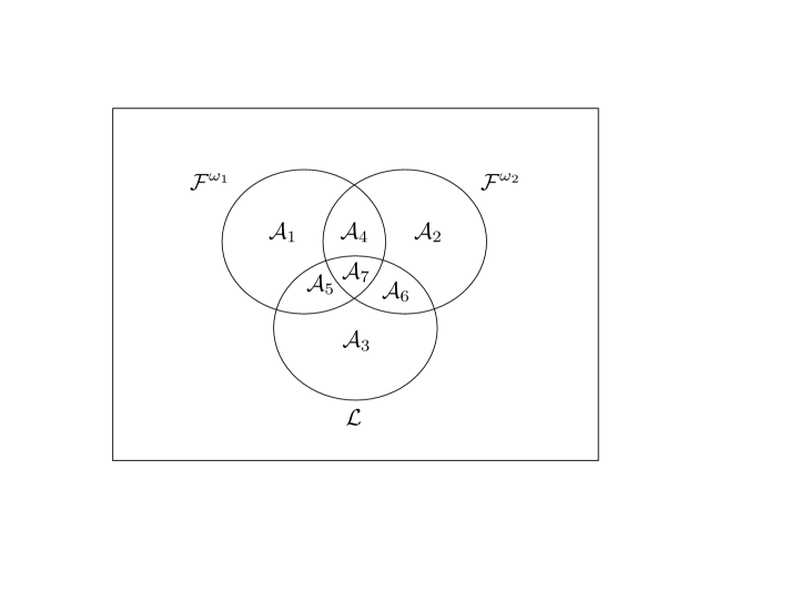
Figure 1: Different sets of functions and their intersections.

Theorem 27

Let $\omega_{1}$, $\omega_{2}$ be arbitrary symplectic forms on $\mathbb{R}^{2n}$ with $\omega_{1}\neq\pm\omega_{2}$. Then the sets $\mathcal{A}_{i}$, $i=1,\cdots,7$ defined as in (165) are all non-empty (see Figure $1$).

Proof. As in [3] we shall suggest ways to construct examples of functions in each of these sets. We start with

${\bf\mathcal{A}_{3}:}$ Consider an arbitrary Gaussian function $\mathcal{G}_{{\bf A}}$ with covariance matrix ${\bf A}$. Clearly $\mathcal{G}_{{\bf A}}\in\mathcal{L}$. Compute the $\omega_{1}$- and $\omega_{2}$-symplectic spectra of ${\bf A}$. Let $\lambda_{max,1}({\bf A})=max\left\{\lambda_{\omega_{1},1}({\bf A}),\lambda_{\omega_{2},1}({\bf A})\right\}$. If $\lambda_{max,1}({\bf A})<\frac{1}{2}$, then $\mathcal{G}_{{\bf A}}\notin\mathcal{F}^{\omega_{1}}\cup\mathcal{F}^{\omega_{2}}$ and we are done. If $\lambda_{max,1}({\bf A})\geq\frac{1}{2}$, then choose some $0<\mu<\frac{1}{2\lambda_{max,1}({\bf A})}$. According to Lemma 16, the Gaussian $\mathcal{G}_{\mu{\bf A}}$ is such that $\lambda_{max,1}(\mu{\bf A})<\frac{1}{2}$ and thus $\mathcal{G}_{\mu{\bf A}}\notin\mathcal{F}^{\omega_{1}}\cup\mathcal{F}^{\omega_{2}}$.

${\bf\mathcal{A}_{7}:}$ Again consider a Gaussian $\mathcal{G}_{{\bf A}}$ with covariance matrix ${\bf A}$ and let $\lambda_{min,1}({\bf A})=min\left\{\lambda_{\omega_{1},1}({\bf A}),\lambda_{\omega_{2},1}({\bf A})\right\}$. If $\lambda_{min,1}({\bf A})\geq\frac{1}{2}$, then $\mathcal{G}_{{\bf A}}\in\mathcal{A}_{7}$. Otherwise, let $\mu\geq\frac{1}{2\lambda_{min,1}({\bf A})}$. Then $\lambda_{min,1}(\mu{\bf A})\geq\frac{1}{2}$ and $\mathcal{G}_{\mu{\bf A}}\in\mathcal{A}_{7}$.

${\bf\mathcal{A}_{5}:}$ According to Theorem 24, there exists a Gaussian $\mathcal{G}_{{\bf A}}$ with covariance matrix ${\bf A}$, such that $\lambda_{\omega_{1},1}({\bf A})>\lambda_{\omega_{2},1}({\bf A})$. Let $\mu$ be such that $2\lambda_{\omega_{1},1}({\bf A})>\mu^{-1}>2\lambda_{\omega_{2},1}({\bf A})$. Then the Gaussian $\mathcal{G}_{\mu{\bf A}}$ is such that $\lambda_{\omega_{1},1}(\mu{\bf A})\geq\frac{1}{2}$, while $\lambda_{\omega_{2},1}(\mu{\bf A})<\frac{1}{2}$. Hence $\mathcal{G}_{\mu{\bf A}}\in\mathcal{A}_{5}$.

${\bf\mathcal{A}_{6}:}$ The result follows the same steps as in $\mathcal{A}_{5}$, with the replacement $\omega_{1}\leftrightarrow\omega_{2}$.

${\bf\mathcal{A}_{1}:}$ Let $h\in\mathcal{F}^{\sigma}\backslash\mathcal{L}$, that is a $\sigma$-Wigner function which is not everywhere nonnegative. Then the function $h_{1}(z)=h({\bf S_{1}}^{-1}z)$ with ${\bf S_{1}}\in\mathcal{D}(n;\omega_{1})$ is in $\mathcal{F}^{\omega_{1}}\backslash\mathcal{L}$. Choose $h_{5}\in\mathcal{A}_{5}$. Since $h_{5}\notin\mathcal{F}^{\omega_{2}}$, there exists $g_{2}\in\mathcal{F}^{\omega_{2}}$, such that (cf.(78)):

$$b:=\int_{\mathbb{R}^{2n}}h_{5}(z)g_{2}(z)dz<0.$$ (166)

Let also

$$a:=\int_{\mathbb{R}^{2n}}h_{1}(z)g_{2}(z)dz.$$ (167)

First suppose that $a\leq 0$. Let $z_{0}\in\mathbb{R}^{2n}$ be such that $h_{1}(z_{0})<0<h_{5}(z_{0})$. Such a $z_{0}$ can always be found because $h_{5}(z)\geq 0$ for all $z$ and is not identically zero. On the other hand if $h_{1}(z)\in\mathcal{F}^{\omega_{1}}\backslash\mathcal{L}$, then $h_{1}(z-\zeta)\in\mathcal{F}^{\omega_{1}}\backslash\mathcal{L}$ for any fixed $\zeta$. So we can always translate $h_{1}$ so that $h_{1}(z_{0})<0$. Next, choose $1>p>0$ such that

$$\frac{p}{1-p}>\frac{h_{5}(z_{0})}{|h_{1}(z_{0})|}.$$ (168)

The function

$$f_{1}(z)=ph_{1}(z)+(1-p)h_{5}(z)$$ (169)

being a convex combination of $h_{1},h_{5}\in\mathcal{F}^{\omega_{1}}$ also belongs to $\mathcal{F}^{\omega_{1}}$. Moreover, since by (168), $f_{1}(z_{0})<0$, we also have $f_{1}\notin\mathcal{L}$. Finally from (166,167):

$$\int_{\mathbb{R}^{2n}}f_{1}(z)g_{2}(z)dz=pa+(1-p)b<0,$$ (170)

and thus $f_{1}\notin\mathcal{F}^{\omega_{2}}$. Altogether, $f_{1}\in\mathcal{A}_{1}$.

Now suppose that we have instead $a>0$. We start by showing that, by translating $h_{1}(z)\mapsto T_{\zeta}h_{1}(z)=h_{1}(z-\zeta)$ appropriately , we can always find $z_{1}\in\mathbb{R}^{2n}$ such that

$$T_{\zeta}h_{1}(z_{1})<0<\frac{h_{5}(z_{1})}{|b|}<\frac{|\left(T_{\zeta}h_{1}\right)(z_{1})|}{a}.$$ (171)

Indeed, let $z_{2}\in\mathbb{R}^{2n}$ be such that $h_{1}(z_{2})<0$ and $z_{1}$ such that

$$0<h_{5}(z_{1})<(2\pi)^{n}|bh_{1}(z_{2})|.$$ (172)

It is always possible to find such a $z_{1}$ because we may assume, without compromising our argument, that $h_{5}\in\mathcal{S}(\mathbb{R}^{2n})$. If $\zeta=z_{1}-z_{2}$, then we have from equation (172), the Cauchy-Schwartz inequality, the purity condition (54), and by replacing $h_{1}$ by $T_{\zeta}h_{1}$ in (167):

$$\begin{array}[]{c}0<\frac{h_{5}(z_{1})}{|b|}a=\frac{h_{5}(z_{1})}{|b|}\left|\int_{\mathbb{R}^{2n}}T_{\zeta}h_{1}(z)g_{2}(z)\right|\leq\\ \\ \leq\frac{h_{5}(z_{1})}{|b|}||T_{\zeta}h_{1}||_{L^{2}}||g_{2}||_{L^{2}}\leq\frac{h_{5}(z_{1})}{(2\pi)^{n}|b|}<|h_{1}(z_{2})|=|T_{\zeta}h_{1}(z_{1})|,\end{array}$$ (173)

which proves (171) for $T_{\zeta}h_{1}$.

From (171) we can choose $p\in\mathbb{R}$ such that

$$0<\frac{\alpha}{1+\alpha}<p<\frac{\beta}{1+\beta}<1,$$ (174)

with

$$0<\alpha=\frac{h_{5}(z_{1})}{|\left(T_{\zeta}h_{1}\right)(z_{1})|}<\frac{|b|}{a}=\beta.$$ (175)

This is because the function $x\in\mathbb{R}^{+}\mapsto\frac{x}{1+x}$ is strictly increasing.

Next, let $f_{1}\in\mathcal{F}^{\omega_{1}}$ be defined as in (169) with $h_{1}$ replaced by $T_{\zeta}h_{1}$. Since

$$f_{1}(z_{1})=-p|\left(T_{\zeta}h_{1}\right)(z_{1})|+(1-p)h_{5}(z_{1})<0$$ (176)

we have $f_{1}\notin\mathcal{L}$. Similarly:

$$\int_{\mathbb{R}^{2n}}f_{1}(z)g_{2}(z)dz=pa-(1-p)|b|<0,$$ (177)

and thus $f_{1}\notin\mathcal{F}^{\omega_{2}}$. Altogether $f_{1}\in\mathcal{A}_{1}$.

${\bf\mathcal{A}_{2}:}$ The result follows the same steps as in $\mathcal{A}_{1}$, with the replacement $\omega_{1}\leftrightarrow\omega_{2}$.

${\bf\mathcal{A}_{4}:}$ To simplify the argument, we start by noticing that proving that $f_{4}\in\mathcal{A}_{4}$ is equivalent to proving that $g_{4}\in\left(\mathcal{F}^{\sigma}\cap\mathcal{F}^{\omega}\right)\backslash\mathcal{L}$ where $g_{4}(z)=f_{4}({\bf S_{1}}z)$, $\omega(z,z^{\prime})=z\cdot{\bf\Omega}^{-1}z^{\prime}$, ${\bf\Omega}={\bf S_{1}}^{-1}{\bf\Omega_{2}}({\bf S_{1}}^{-1})^{T}$ with ${\bf S_{1}}\in\mathcal{D}(n;\omega_{1})$, ${\bf S_{2}}\in\mathcal{D}(n;\omega_{2})$. Indeed, $f_{4}\notin\mathcal{L}\Leftrightarrow g_{4}\notin\mathcal{L}$. Moreover, $f_{4}(z)\in\mathcal{F}^{\omega_{1}}\Leftrightarrow g(z)=f_{4}({\bf S_{1}}z)\in\mathcal{F}^{\sigma}$. Finally, $f_{4}(z)\in\mathcal{F}^{\omega_{2}}\Leftrightarrow f_{4}({\bf S_{2}}z)=g_{4}({\bf S_{1}}^{-1}{\bf S_{2}}z)\in\mathcal{F}^{\sigma}$. But since ${\bf S_{1}}^{-1}{\bf S_{2}}\in\mathcal{D}(n;\omega)$, this is equivalent to $g_{4}\in\mathcal{F}^{\omega}$.

Let us now devise a way to construct a function $g_{4}\in\left(\mathcal{F}^{\sigma}\cap\mathcal{F}^{\omega}\right)\backslash\mathcal{L}$. Consider the function

$$\gamma(\alpha)=\det({\bf J}-\alpha{\bf\Omega}).$$ (178)

We claim that there exists $\alpha_{0}>1$ such that

$$\gamma_{0}:=\gamma(\alpha_{0})>0.$$ (179)

Indeed, $\gamma(\alpha)=\det\left({\bf J\Omega^{-1}}-\alpha{\bf I}\right)$. Thus $\gamma$ is the characteristic polynomial of the matrix ${\bf J\Omega^{-1}}$. We thus have:

$$\begin{array}[]{c}\gamma(\alpha)=\alpha^{2n}+Tr\left({\bf J\Omega^{-1}}\right)\alpha^{2n-1}+\cdots+\det\left({\bf J\Omega^{-1}}\right)=\\ \\ =\alpha^{2n}+Tr\left({\bf J\Omega^{-1}}\right)\alpha^{2n-1}+\cdots+1.\end{array}$$ (180)

Hence $\gamma(\alpha)\simeq\alpha^{2n}$ as $\alpha\to+\infty$, which proves the claim. Define ${\bf\Sigma_{1}}={\bf\Omega}$ and ${\bf\Sigma_{2}}=\gamma_{0}^{-\frac{1}{2n}}({\bf J}-\alpha_{0}{\bf\Omega})$ and the corresponding normalized symplectic forms:

$$\eta_{1}=\omega,\hskip 28.45274pt\eta_{2}(z,z^{\prime})=z\cdot{\bf\Sigma_{2}^{-1}}z^{\prime}.$$ (181)

We claim that there exists ${\bf A}\in\mathbb{P}^{\times}_{2n\times 2n}(\mathbb{R})$ such that

$$\lambda_{\eta_{1},1}({\bf A})=\alpha_{0}-1,$$ (182)

and

$$\lambda_{\eta_{2},1}({\bf A})\geq\gamma_{0}^{\frac{1}{2n}}.$$ (183)

Indeed, from Theorem 24, we can find ${\bf A}\in\mathbb{P}^{\times}_{2n\times 2n}(\mathbb{R})$ such that

$$\frac{\lambda_{\eta_{2},1}({\bf A})}{\lambda_{\eta_{1},1}({\bf A})}\geq\frac{\gamma_{0}^{\frac{1}{2n}}}{\alpha_{0}-1}.$$ (184)

After a possible rescaling ${\bf A}\mapsto\mu{\bf A}$ $(\mu>0)$, we obtain (182) and (183) follows from (184).

Conditions (182,183) mean that

$${\bf A}+i(\alpha_{0}-1){\bf\Omega}\geq 0,$$ (185)

while

$${\bf A}+i\alpha_{0}{\bf\Omega}\ngeq 0.$$ (186)

On the other hand, we also have

$${\bf A}+i\gamma_{0}^{\frac{1}{2n}}{\bf\Sigma_{2}}\geq 0.$$ (187)

Next, let $h^{\sigma}$ be a non-Gaussian pure state with Planck constant $\alpha_{0}$, that is (cf. item 6 of Theorem 11)

$$\mathcal{W}^{{\bf J}}(\mathcal{F}h^{\sigma})=\left\{-\alpha_{0},\alpha_{0}\right\}.$$ (188)

Given ${\bf S}\in\mathcal{D}(n;\omega)$, let $h^{\omega}(z)=h^{\sigma}({\bf S^{-1}}z)$. From Remark 9:

$$\left\{-\alpha_{0},\alpha_{0}\right\}\subset\mathcal{W}^{{\bf\Omega}}(\mathcal{F}h^{\omega}).$$ (189)

If $\mathcal{G}_{{\bf A}}$ is a Gaussian with covariance matrix ${\bf A}$, then from (185-187):

$$(\alpha_{0}-1,{\bf\Omega}),(\gamma_{0}^{\frac{1}{2n}},{\bf\Sigma_{2}})\in\mathcal{W}(\mathcal{F}\mathcal{G}_{{\bf A}}),$$ (190)

but

$$(\alpha_{0},{\bf\Omega})\notin\mathcal{W}(\mathcal{F}\mathcal{G}_{{\bf A}}).$$ (191)

Given (191), we can always find $h^{\sigma}\notin\mathcal{L}$ such that

$$g_{4}=\mathcal{G}_{{\bf A}}\star h^{\omega}\notin\mathcal{L}.$$ (192)

Indeed, we have for ${\bf S}\in\mathcal{D}(n;\omega)$:

$$\begin{array}[]{c}g_{4}({\bf S}z)=(\mathcal{G}_{{\bf A}}\star h^{\omega})({\bf S}z)=\int_{\mathbb{R}^{2n}}\mathcal{G}_{{\bf A}}({\bf S}z-z^{\prime})h^{\omega}(z^{\prime})dz^{\prime}=\\ \\ =\int_{\mathbb{R}^{2n}}\mathcal{G}_{{\bf A}}({\bf S}(z-z^{\prime\prime}))h^{\omega}({\bf S}z^{\prime\prime})dz^{\prime\prime}=\\ \\ =\int_{\mathbb{R}^{2n}}\mathcal{G}_{{\bf S}^{-1}{\bf A}({\bf S}^{-1})^{T}}(z-z^{\prime\prime})h^{\sigma}(z^{\prime\prime})dz^{\prime\prime}.\end{array}$$ (193)

Since ${\bf S}^{-1}{\bf A}({\bf S}^{-1})^{T}+i\alpha_{0}{\bf J}={\bf S}^{-1}\left({\bf A}+i\alpha_{0}{\bf\Omega}\right)({\bf S}^{-1})^{T}$, from (186) this is not a positive matrix. Consequently, the Gaussian $\mathcal{G}_{{\bf S}^{-1}{\bf A}({\bf S}^{-1})^{T}}(z)$ is not a $\sigma$-Wigner function with Planck constant $\alpha_{0}$. It is a well known fact that, under these circumstances [49, 50], the function $h^{\sigma}\notin\mathcal{L}$, which is a Wigner function with Planck constant $\alpha_{0}$ can always be chosen so that $(\mathcal{G}_{{\bf A}}\star h^{\omega})({\bf S}z)=(\mathcal{G}_{{\bf S}^{-1}{\bf A}({\bf S}^{-1})^{T}}\star h^{\sigma})(z)\notin\mathcal{L}$.

We thus have for the function

$$g_{4}(z)=(\mathcal{G}_{{\bf A}}\star h^{\omega})(z)$$ (194)

that $g_{4}\notin\mathcal{L}$.

Next, notice that ${\bf S}^{-1}{\bf A}({\bf S}^{-1})^{T}+i(\alpha_{0}-1){\bf J}\geq 0$, and so $(\alpha_{0}-1,{\bf J})\in\mathcal{W}(\mathcal{F}\mathcal{G}_{{\bf S}^{-1}{\bf A}({\bf S}^{-1})^{T}})$. Since $(1-\alpha_{0},{\bf J})\oplus(\alpha_{0},{\bf J})=(1,{\bf J})$, we conclude from (193) and Theorem 10 that $g_{4}({\bf S}z)$ is of the $(1,{\bf J})$-positive type. And thus $g_{4}(z)\in\mathcal{F}^{\omega}$.

It remains to prove that $g_{4}(z)\in\mathcal{F}^{\sigma}$. Since $(\gamma_{0}^{\frac{1}{2n}},{\bf\Sigma_{2}})\oplus(\alpha_{0},{\bf\Omega})=(1,{\bf J})$, the result follows again from Theorem 10.   

We conclude this subsection by applying the previous techniques to the following representability problem. This completes the discussion initiated in [26] and addressed also in Theorem 25.

Theorem 28

Let $\omega_{1}(z,z^{\prime})=z\cdot{\bf\Omega_{1}^{-1}}z^{\prime}$ be a symplectic form and suppose that ${\bf M}\in Gl(2n;\mathbb{R})$ is not $\omega_{1}$-symplectic nor $\omega_{1}$-anti-symplectic. Define $\omega_{2}(z,z^{\prime})=z\cdot{\bf\Omega_{2}^{-1}}z^{\prime}$ where ${\bf\Omega_{2}}=\frac{1}{\alpha}{\bf M\Omega_{1}M^{T}}$, with $\alpha=|\det{\bf M}|^{\frac{1}{n}}$. Consider again the linear operator $\mathcal{U}_{{\bf M}}$ as defined in (5). Then there exist $W^{\omega_{1}}\rho\in\mathcal{F}^{\omega_{1}}$ such that $\mathcal{U}_{{\bf M}}(W^{\omega_{1}}\rho)\in\mathcal{F}^{\omega_{1}}\cap\mathcal{F}^{\omega_{2}}$ and $W^{\omega_{1}}\rho^{\prime}\in\mathcal{F}^{\omega_{1}}$ such that $\mathcal{U}_{{\bf M}}(W^{\omega_{1}}\rho^{\prime})\in\mathcal{F}^{\omega_{2}}\backslash\mathcal{F}^{\omega_{1}}$.

Proof. We follow the strategy used in the proof of the previous theorem for the cases $\mathcal{A}_{5}$ and $\mathcal{A}_{7}$. We just have to be cautious because we do not have necessarily $|\det{\bf M}|=1$.

So let $W^{\omega_{1}}\rho=\mathcal{G}_{{\bf A}}$ be a Gaussian (89) with covariance matrix ${\bf A}$ such that

$${\bf A}+\frac{i}{2}{\bf\Omega_{1}}\geq 0.$$ (195)

Since

$$\mathcal{U}_{{\bf M}}(\mathcal{G}_{{\bf A}})=\mathcal{G}_{{\bf M^{-1}}{\bf A}({\bf M^{-1}})^{T}},$$ (196)

we conclude that $\mathcal{U}_{{\bf M}}(W^{\omega_{1}}\rho)\in\mathcal{F}^{\omega_{1}}$ if and only if

$${\bf M^{-1}}{\bf A}({\bf M^{-1}})^{T}+\frac{i}{2}{\bf\Omega_{1}}\geq 0\Leftrightarrow{\bf A}+\frac{i\alpha}{2}{\bf\Omega_{2}}\geq 0.$$ (197)

Since ${\bf M}$ is not a $\omega_{1}$-symplectic or a $\Omega_{2}$-antisymplectic matrix, then $\omega_{2}\neq\pm\omega_{1}$. The matrix ${\bf A}$ satisfies (195) and (197) if and only if $\lambda_{\omega_{1},1}({\bf A})\geq\frac{1}{2}$ and $\lambda_{\omega_{2},1}({\bf A})\geq\frac{\alpha}{2}$. From the case $\mathcal{A}_{7}$ of the previous theorem we already know how to construct such a matrix after a possible rescaling.

Regarding the function $W^{\omega_{1}}\rho^{\prime}$ we assume that it is again a Gaussian $\mathcal{G}_{{\bf B}}$ with covariance matrix ${\bf B}$. It is a $\omega_{1}$-Wigner function if and only if

$${\bf B}+\frac{i}{2}{\bf\Omega_{1}}\geq 0,$$ (198)

and $\mathcal{U}_{{\bf M}}(W^{\omega_{1}}\rho^{\prime})\in\mathcal{F}^{\omega_{2}}\backslash\mathcal{F}^{\omega_{1}}$ provided

$${\bf B}+\frac{i\alpha}{2}{\bf\Omega_{2}}\ngeqslant 0.$$ (199)

Again, this happens if and only if $\lambda_{\omega_{1},1}({\bf B})\geq\frac{1}{2}$ and $\lambda_{\omega_{2},1}({\bf B})<\frac{\alpha}{2}$. From the case $\mathcal{A}_{5}$ of the previous theorem, we know that such a matrix exists.   

***************************************************************

Author’s addresses:

Nuno Costa Dias and João Nuno Prata: Escola Superior Náutica Infante D. Henrique. Av. Eng. Bonneville Franco, 2770-058 Paço d’Arcos, Portugal and Grupo de Física Matemática, Universidade de Lisboa, Av. Prof. Gama Pinto 2, 1649-003 Lisboa, Portugal

***************************************************************

References

- [1] M.J. Bastiaans: Wigner distribution function and its application to first order optics. J. Opt. Soc. Amer. 69 (1979) 1710-1716.
- [2] C. Bastos, O. Bertolami, N.C. Dias, and J.N. Prata: Weyl–Wigner Formulation of Noncommutative Quantum Mechanics, J. Math. Phys. 49 (2008) 072101.
- [3] C. Bastos, N.C. Dias, and J.N. Prata: Wigner measures in noncommutative quantum mechanics, Comm. Math. Phys. 299 (2010), no.3, 709–740.
- [4] C. Bastos, O. Bertolami, N.C. Dias, and J.N. Prata: Black holes and phase-space noncommutativity. Phys. Rev. D 80 (2009) 124038.
- [5] C. Bastos, O. Bertolami, N.C. Dias, and J.N. Prata: Phase-space noncommutative quantum cosmology. Phys. Rev. D 78 (2008) 023516.
- [6] C. Bastos, O. Bertolami, N.C. Dias, and J.N. Prata: Singularity problem and phase-space noncanonical noncommutativity. Phys. Rev. D 82 (2010) 041502 (R).
- [7] C. Bastos, A. Bernardini, O. Bertolami, N.C. Dias, and J.N. Prata: Entanglement due to noncommutativity in phase space. Phys. Rev. D 88 (2013) 085013.
- [8] C. Bastos, O. Bertolami, N.C. Dias, and J.N. Prata: Violation of the Robertson-Schrödinger uncertainty principle and noncommutative quantum mechanics. Phys. Rev. D 86 (2012) 105030.
- [9] F. Bayen, M. Flato, C. Fronsdal, A. Lichnerowicz, D. Sternheimer: Deformation theory and quantization I. Deformations of symplectic structures. Ann. Phys. (N.Y.) 111 (1978) 61-110.
- [10] J. Bellissard, A. van Elst, H. Schulz-Baldes: The non-commutative geometry of the quantum hall effect. J. Math. Phys. 35 (1994) 5373-5451.
- [11] K. Bolonek, P. Kosinski: On uncertainty relations in noncommutative quantum mechanics. Phys. Lett. B 547 (2002) 51-54.
- [12] A. Borowiec, A. Pachol: Twisted bialgebroids from a Drinfeld twist. J. Phys. A: Math. Theor. 50 (2017) 055205.
- [13] A. Bracken, G. Cassinelli, J. Wood: Quantum symmetries and the Weyl-Wigner product of group representations. J. Phys. A: Math. Gen. 36(4) (2003) 1033.
- [14] S.L. Braunstein, P. van Loock: Quantum information with continuous variables. Rev. Mod. Phys. 77 (2005) 513-577.
- [15] T. Bröcker, R.F. Werner: Mixed states with positive Wigner functions. J. Math. Phys. 36 (1995) 62.
- [16] A. Cannas da Silva: Lectures on symplectic geometry. Springer (2001).
- [17] S.M. Carroll, J.A. Harvey, V.A. Kostelecký, C.D. Lane, T. Okamoto: Noncommutative field theory and Lorentz violation. Phys. Rev. Lett. 87 (2001) 141601.
- [18] S.H.H. Chowdhuri, and S.T. Ali: Wigner functions for noncommutative quantum mechanics: a group representation based construction. J. Math. Phys. 56 (2015) 122102.
- [19] S.H.H. Chowdhuri, and S.T. Ali: Triply extended group of translations of as defining group of NCQM: relations to various gauges. J. Phys. A: Math. Theo. 47 (2014) 085301.
- [20] L. Cohen, P. Loughlin, G. Okopal: Exact and approximate moments of a propagating pulse. J. Mod. Optics 55 (2008) 3349-3358.
- [21] A. Connes: Noncommutative Geometry. London-New York: Academic Press, 1994.
- [22] F. Delduc, Q. Duret, F. Gieres, M. Lefranccois: Magnetic fields in noncommutative quantum mechanics. J. Phys. Conf. Ser. 103 (2008) 012020.
- [23] M. Demetrian, D. Kochan: Quantum mechanics on noncommutative plane. Acta Phys. Slov. 52 (2002) 1.
- [24] N.C. Dias, M. de Gosson, F. Luef, J.N. Prata: A Deformation Quantization Theory for Non-Commutative Quantum Mechanics, J. Math. Phys. 51 (2010) 072101 (12 pages).
- [25] N.C. Dias, M. de Gosson, F. Luef, J.N. Prata: A pseudo–differential calculus on non–standard symplectic space; spectral and regularity results in modulation spaces. J. Math. Pures Appl. 96 (2011) 423–445
- [26] N.C. Dias, M. de Gosson, J.N. Prata: Maximal covariance group of Wigner transforms and pseudo-differential operators. Proc. Amer. Math. Soc. 142 (2014) 3183–3192
- [27] N.C. Dias, J.N. Prata: Admissible states in quantum phase space. Ann. Phys.(N. Y.), 313 (2004) 110–146.
- [28] N.C. Dias, J.N. Prata: The Narcowich-Wigner spectrum of a pure state. Rep. Math. Phys. 63 (2009) 43–54.
- [29] N.C. Dias, J.N. Prata: Exact master equation for a noncommutative Brownian particle. Ann. Phys. (N.Y.) 324 (2009) 73-96.
- [30] M.R. Douglas, N.A. Nekrasov: Noncommutative field theory. Rev. Mod. Phys. 73 (2001) 977.
- [31] D. Dubin, M. Hennings, T. Smith: Mathematical aspects of Weyl quantization. Singapore: World Scientific, 2000.
- [32] C. Duval, P.A. Horvathy: Exotic galilean symmetry in the noncommutative plane and the Landau effect. J. Phys. A: Math. Gen. 34 (2001) 10097.
- [33] D. Ellinas, A.J. Bracken: Phase-space-region operators and the Wigner function: geometric constructions and tomography. Phys. Rev. A 78 (2008) 052106.
- [34] B. Fedosov: A simple geometric construction of deformation quantization. J. Diff. Geom. 40 (1994) 213.
- [35] B. Fedosov: Deformation quantization and index theory. Berlin: Akademie Verlag, 1996.
- [36] G. B. Folland: Harmonic Analysis in Phase space. Annals of Mathematics studies, Princeton University Press, Princeton, N.J. (1989).
- [37] J. Gamboa, M. Loewe, J.C. Rojas: Noncommutative quantum mechanics. Phys. Rev. D 64 (2001) 067901.
- [38] H. García-Compeán, O. Obregón, C. Ramírez: Noncommutative quantum cosmology. Phys. Rev. Lett. 88 (2002) 161301.
- [39] D.Giulini, E. Joos, C. Kiefer, J. Kupsch, I.-O. Stamatescu, H.D. Zeh: Decoherence and the appearence of a classical world in quantum theory. Springer (1996).
- [40] M. de Gosson. Symplectic Geometry and Quantum Mechanics, Birkhäuser, Basel, series “Operator Theory: Advances and Applications” (subseries: “Advances in Partial Differential Equations”), Vol. 166 (2006)
- [41] M. de Gosson. Symplectic Methods in Harmonic Analysis ans in Mathematical Physics, Birkhäuser, Basel, series “Pseudo-Differential Operators: Theory and Applications”, Vol. 7 (2010).
- [42] M. de Gosson: Maslov indices on the metaplectic group Mp(n). Ann. Inst. Four. 40 (1990) 537-555.
- [43] M. de Gosson: Symplectic covariance properties for Shubin and Born-Jordan pseudo-differential operators. Trans. Amer. Math. Soc. 365 (2013) 3287-3307.
- [44] G. Grubb: Distributions and operators. Berlin-Heidelberg-New York: Springer, 2009.
- [45] M. Henneaux, C. Teitelbaum: Quantization of gauge systems. Princeton University Press (1992).
- [46] L. Hörmander: The analysis of linear partial differential operators I. Berlin-Heidelberg-New York: Springer-Verlag, 1983.
- [47] P.A. Horvathy: The noncommutative Landau problem. Ann. Phys. (N.Y.) 299 (2002) 128.
- [48] R.L. Hudson: When is the Wigner quasi-probability density non-negative? Rep. Math. Phys. 6 (1974) 249-252.
- [49] A.J.E.M. Janssen: A note on Hudson’s Theorem about functions with nonnegative Wigner distributions. SIAM J. Math. Anal. 15 (1984) 170.
- [50] A.J.E.M. Janssen: Positivity of weighted Wigner distributions. SIAM J. Math. Anal. 12 (1981) 752.
- [51] J.-J. Jiang, S.H.H. Chowdhuri: Deformation of noncommutative quantum mechanics. Arxiv: math-ph: 1603.05805.
- [52] D. Kastler, The -algebras of a free boson field. Commun. Math. Phys. 1 (1965) 14.
- [53] M. Kontsevich: Deformation quantization of Poisson manifolds. Lett. Math. Phys. 66 (2003) 157.
- [54] J. Leray: Lagrangian analysis and quantum mechanics. A mathematical structure related to asymptotic expansions and the Maslov index. MIT Press, Cambridge, Mass. (1981).
- [55] P.L. Lions, T. Paul: Sur les mesures de Wigner. Rev. Mat. Iberoamer. 9 (1993) 553-618.
- [56] R.G. Littlejohn: The semiclassical evolution of wave packets. Phys. Rep. 138 (1986) 193.
- [57] P. Loughlin, L. Cohen: Approximate wavefunction from approximate non-representable Wigner distributions. J. Mod. Optics 55 (2008) 3379-3387.
- [58] G. Loupias, S. Miracle-Sole: -algèbres des systèmes canoniques. Ann. Inst. H. Poincaré 6 (1967) 39.
- [59] J. Madore: An introduction to noncommutative differential geometry and its physical applications. 2nd Edition. Cambridge: Cambridge University Press (2000).
- [60] B. Malekolkalami, M. Farhoudi: Noncommutative double scalar fields in FRW cosmology as cosmical oscillators. Class. Quant. Grav. 27 (2010) 245009.
- [61] A. Martinez: An introduction to semiclassical and microlocal analysis. Springer (2002).
- [62] L. Monreal, P. Fernández de Córdoba, A. Ferrando, J.M. Isidro: Noncommutative space and the low-energy physics of quasicrystrals. Int. J. Mod. Phys. A 23 (2008) 2037-2045.
- [63] J.E. Moyal: Quantum mechanics as a statistical theory. Proc. Cambr. Phil. Soc. 45 (1949) 99-124.
- [64] V.P. Nair, A.P. Polychronakos: Quantum mechanics on the noncommutative plane and sphere. Phys. Lett. B 505 (2001) 267.
- [65] M. Nakamura: Star-product description of qunatization in second-class constraint systems. Arxiv: math-ph/1108.4108 (2011).
- [66] M. Nakamura: Canonical structure of noncommutative quantum mechanics as constraint system. Arxiv: hep-th/1402.2132 (2014).
- [67] F.J. Narcowich: Conditions for the convolution of two Wigner distributions to be itself a Wigner distribution. J. Math. Phys. 29 (1988) 2036.
- [68] P. Nicolini, A. Smailagic, E. Spallucci: Noncommutative geometry inspired Schwarzschild black hole. Phys. Lett. B 632 (2006) 547-551.
- [69] J.C. Pool: Mathematical aspects of the Weyl correspondence. J. Math. Phys. 7 (1966) 66.
- [70] M. Reed, B. Simon: Methods in Modern Mathematical Physics. Vol. 1: Functional Analysis. Academic Press. Elsevier (1980).
- [71] C. Rovelli: Quantum gravity. Cambridge University Press (2004).
- [72] N. Seiberg, E. Witten: String theory and noncommutative geometry. JHEP 9909 (1999) 032.
- [73] D. Shale: Linear symmetries of free boson fields. Trans. Amer. Math. Soc. 103 (1062) 149-167.
- [74] R. Simon: Peres-Horodecki separability criterion for continuous variable systems. Phys. Rev. Lett. 84 (2000) 2726.
- [75] F. Soto, P. Claverie: When is the Wigner function of multidimensional systems nonnegative? J. Math. Phys. 24 (1983) 97.
- [76] R.J. Szabo: Quantum field theory on noncommutative spaces. Phys. Rept. 378 (2003) 207-299.
- [77] J. Toseik: The eigenvalue equation for a 1-D Hamilton function in deformation quantization. Phys. Lett. A 376 (2012) 2023-2031.
- [78] R. Vilela Mendes: Deformations, stable theories and fundamental constants. J. Phys. A: Math. Gen. 27 (1994) 8091-8104.
- [79] A. Weil: Sur certains groupes d’opérateurs unitaires. Acta. Math. 111 (1964) 143-211.
- [80] R.F. Werner, M.M. Wolf: Bound entangled Gaussian states. Phys. Rev. Lett. 86 (2001) 3658.
- [81] E. Wigner: On the quantum correction for for thermodynamics equilibrium. Phys. Rev. 40 (1932) 749.
- [82] M. Wilde, P. Lecomte: Existence of star-products and of formal deformations of the Poisson Lie algebra of arbitrary symplectic manifolds. Lett. Math. Phys. 7 (1983) 487.
- [83] J. Williamson: On the algebraic problem concerning the normal forms of linear dynamical systems. Amer. J. Math. 58 (1936) 141-163.
- [84] M. W. Wong. Weyl Transforms. Springer (1998).
- [85] M. Zworski: Semi-classical analysis. Graduate studies in mathematics 138. American Mathematical Society, Providence (2012).
***************************************************************