Multi-Task Spatiotemporal Neural Networks
for Structured Surface Reconstruction

Abstract

Deep learning methods have surpassed the performance of traditional techniques on a wide range of problems in computer vision, but nearly all of this work has studied consumer photos, where precisely correct output is often not critical. It is less clear how well these techniques may apply on structured prediction problems where fine-grained output with high precision is required, such as in scientific imaging domains. Here we consider the problem of segmenting echogram radar data collected from the polar ice sheets, which is challenging because segmentation boundaries are often very weak and there is a high degree of noise. We propose a multi-task spatiotemporal neural network that combines 3D ConvNets and Recurrent Neural Networks (RNNs) to estimate ice surface boundaries from sequences of tomographic radar images. We show that our model outperforms the state-of-the-art on this problem by (1) avoiding the need for hand-tuned parameters, (2) extracting multiple surfaces (ice-air and ice-bed) simultaneously, (3) requiring less non-visual metadata, and (4) being about 6 times faster.

1 Introduction

Three-dimensional imaging is widely used in scientific research domains (e.g., biology, geology, medicine, and astronomy) to characterize the structure of objects and how they change over time. Although the exact techniques differ depending on the problem and materials involved, the common idea is that electromagnetic waves (e.g., X-ray, radar, etc.) are sent into an object, and signal returns in the form of sequences of tomographic images are then analyzed to estimate the object’s 3D structure. However, analysis of these image sequences can be difficult even for humans, since they are often noisy and require integrating evidence from multiple sources simultaneously.

Figure 1: Illustration of our task. A ground-penetrating radar system flies over a polar ice sheet, yielding a sequence of 2D tomographic slices (e.g. Sample (a) with the black dashed bounding box). Each slice captures a vertical cross-section of the ice, where two material boundaries (the ice-air and ice-bed layer) are visible as bright curves in the radar echogram. Given such a sequence of tomographic slices, our goal is to reconstruct the 3D surfaces for each material boundary (e.g. a sample ice-bed surface [35] is shown in the figure).

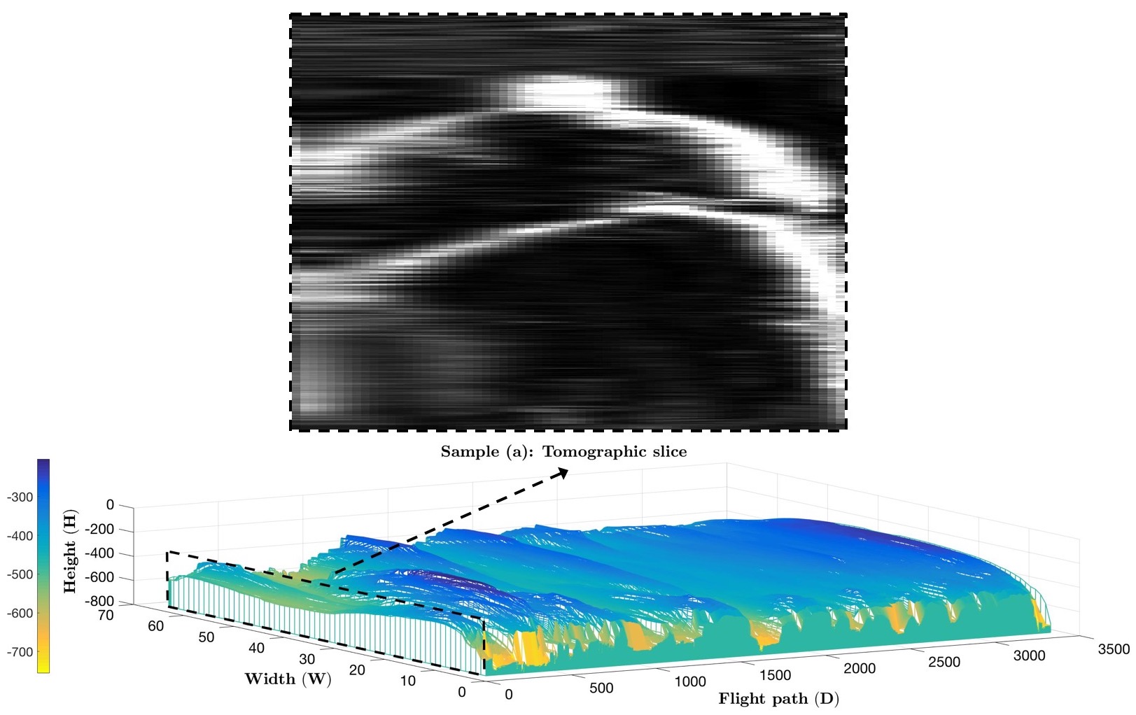
As a particular example, an important part of modeling and forecasting the effects of global climate change is to understand polar ice. Hidden beneath the ice of the poles is a rich and complex structure: the ice consists of multiple layers that have accumulated over many thousands of years, and the base is bedrock that has a complicated topography just like any other place on Earth (with mountains, valleys, and other features). Moreover, the ice sheets move over time, and their movement is determined by a variety of factors, including temperature changes, flows underneath the surface, and the topography of the bedrock below and nearby. Accurately estimating all of this rich structure is crucial for understanding how ice will change over time, which in turn is important for predicting the effects of melting ice associated with climate change.

Glaciologists traditionally had to drill ice cores to probe the subsurface structure of polar ice, but advances in ground-penetrating radar technology have revolutionized this data collection process. But while these radar observations can now be collected over very large areas, actually analyzing the radar data to determine the structure of subsurface ice is typically done by hand [24]. This is because the radar echograms produced by the data collection process are very noisy: thermal radiation, electromagnetic interference, complex ice composition, and signal attenuation in ice, etc. affect radar signal returns in complex ways. Relying on humans to interpret data not only limits the rate at which datasets can be processed, but also limits the type of analysis that can be performed: while a human expert can readily mark ice sheet boundaries in a single 2D radar echogram, doing this simultaneously over thousands of echograms to produce a 3D model of an ice bed, for example, is simply not feasible.

While several recent papers have proposed automated techniques for segmenting layer boundaries in ice [13, 17, 12, 25, 8, 23, 5, 35, 26], none have approached the accuracy of even an undergraduate student annotator [24], much less an expert. However, these techniques have all relied on traditional image processing and computer vision techniques, like edge detection, pixel template models, active contour models, etc. Most of these techniques also rely on numerous parameters and thresholds that must be tuned by hand. Some recent work reduces the number of free parameters through graphical models that explicitly model noise and uncertainty [35, 23, 8, 26] but still rely on simple features.

In this paper, we apply deep networks to the problem of ice boundary reconstruction in polar radar data. Deep networks have become the de facto standard technique across a wide range of vision tasks, including pixel labeling problems. The majority of these successes have been on consumer-style images, where there is substantial tolerance for incorrect predictions. In contrast, for problems involving scientific datasets like ice layer finding, there is typically only one “correct” answer, and it is important that the algorithm’s output be as accurate as possible.

Here we propose a technique for combining 3D convolutions and Recurrent Neural Networks (RNNs) to perform segmentation in 3D, borrowing techniques usually used for video analysis to instead characterize sequences of tomographic slice images. In particular, since small pixel value changes only affect a few adjacent images, we apply 3D convolutional neural networks to efficiently capture cross-slice features. We extract these spatial and temporal features for small neighborhoods of slices, and then apply an RNN for detailed structure labeling across the entire 2D image. Finally, layers from multiple images are concatenated to generate a 3D surface estimate. We test our model on extracting 3D ice subsurfaces from sequences of radar tomographic images, and achieve the state-of-the-art results in both accuracy and speed.

2 Related Work

A number of methods have been developed for detecting layers or surfaces of material boundaries from sequential noisy radar images. For example, in echograms from Mars, Freeman et al. [13] find layer boundaries by applying band-pass filters and thresholds to find linear subsurface structures, while Ferro and Bruzzone [11] identify subterranean features using iterative region-growing. Crandall et al. [8] detect the ice-air and ice-bed layers in individual radar echograms by combining a pre-trained template model and a smoothness prior in a probabilistic graphical model. In order to achieve more accurate and efficient results, Lee et al. [23] utilize Gibbs sampling from a joint distribution over all candidate layers, while Carrer and Bruzzone [5] reduce the computational complexity with a divide-and-conquer strategy. Xu et al. [35] extend the work to the 3D domain to reconstruct 3D subsurfaces using a Markov Random Field (MRF).

In contrast, we are not aware of any work that has studied this application using deep neural networks. In the case of segmenting single radar echograms, perhaps the closest analogue is segmentation in consumer images [32]. Most of this work differs from the segmentation problem we consider here, however, because our data is much noisier, our “objects” are much harder to characterize (e.g., two layers of ice look virtually identical except for some subtle changes in texture or intensity), our labeling problem has greater structure, and our tolerance for errors in the output is lower.

Figure 2: Architecture of our model for predicting multiple ice layers in tomographic images. We extract and reconstruct structured 3D surfaces from sequential data by combining C3D and RNN networks. A C3D network serves as a robust feature extractor to capture both local within-slice and between-slice features in 3D space, and an RNN serves to capture longer-range structure both within individual images and across the entire sequence.

For segmenting 3D regions, perhaps the closest related work is in deep networks for video analysis, where the frames of video can be viewed as similar to our tomographic slices. Papers that apply deep networks to video applications focus on efficient ways to combine spatial and temporal information, and can be roughly categorized into three classes: (1) combining both RGB frames for spatial features and optical flow images for temporal features in two-stream networks [29], (2) explicitly learning 3D spatiotemporal filters on image spaces through techniques such as C3D [31], and (3) various combinations of both [4]. In order to obtain video representations from per-frame or per-video-segment features, it is a common practice to apply temporal pooling to abstract into fixed-length per-video features [20, 29]. These approaches achieve significantly better classification accuracy on video classification compared to traditional approaches using hand-crafted features.

Recurrent Neural Networks (RNNs) and the specific version we consider here – Gated Recurrent Units (GRUs) – have been proposed for learning sequential data, such as natural language sentences [10, 14], programming language syntax [19], and video frames [37]. A popular application of RNNs recently [33, 18] is to generate image captions in combination with CNNs. In this case, CNNs are used to recognize image content while RNNs are used as language models to generate new sentences. Video can also be thought of as sequential data, since adjacent frames share similar content while differences reveal motion and other changes over time. A large variety of studies [37, 9, 27] share the common idea of applying RNNs on deep features for each video frame and pooling or summing over them to create a video descriptor. Other successful applications of RNNs to interesting vision and natural language tasks include recognizing multiple objects by making guided glimpses in different parts of images [3], answering visual questions [2, 34, 22], generating new images with variations [15, 36], reading lips [7], etc.

We build on this existing work but apply to the novel domain of extracting and reconstructing structured 3D surfaces from sequential data by combining C3D and RNN networks. In particular, we use the C3D network as a robust feature extractor to capture local-scale within-slice and between-slice features in 3D space, and use the RNN to capture longer-range structure both within single slices and across the entire image sequence.

3 Technical Approach

Three-dimensional imaging typically involves sending electromagnetic radiation (e.g., radar, X-ray, etc.) into a material and collecting a sequence of cross-sectional tomographic slices $I=\{I_{1},I_{2},\cdots,I_{D}\}$ that characterize returned signals along the path. Each slice $I_{d}$ is a 2D tomographic image of size $H\times W$ pixels. In the particular case of ice segmentation, we are interested in locating $K$ layer surface boundaries between different materials. Our output surfaces are highly structured, since there should be exactly $K$ surface pixels within any column of a given tomographic image. We thus need to estimate the layer boundaries in each individual slice, while incorporating evidence from all slices jointly in order to overcome noise and resolve ambiguities. Layer boundaries within each slice can then be concatenated across slices to produce a 3D surface.

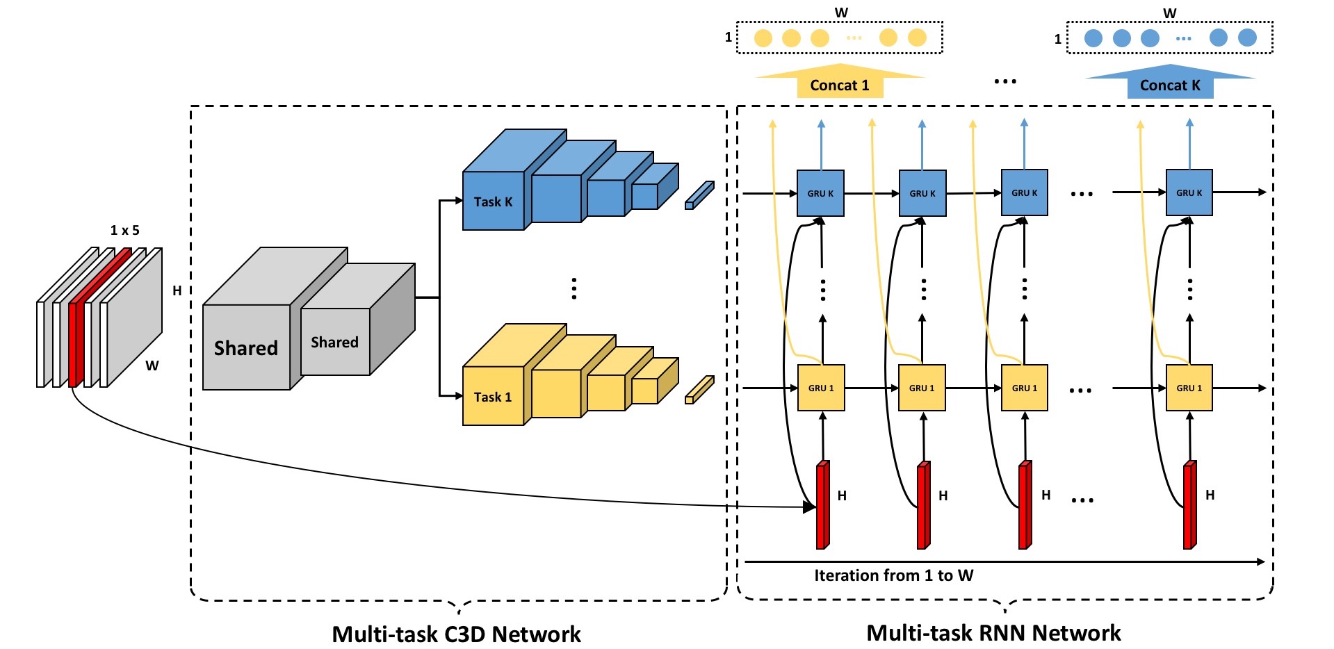
In this section, we describe the two important components of our network framework: our multi-task 3D Convolutional (C3D) Network that captures within-slice features as well as evidence from nearby slices, and our Recurrent Neural Network (RNN) which incorporates longer-range cross-slice constraints. The overall architecture is shown in Figure 2.

Figure 3: Illustration of our C3D architecture in a special case of two layers ($K=2$). All 3D convolution kernels are $3\times 5\times 3$ with stride $1$ in each dimension and the 3D pooling kernels are $1\times 2\times 1$ with stride $2$ in the height dimension of each image.

3.1 A Multi-task C3D Architecture

Traditional convolutional networks for tasks like object classification and recognition lack the ability to model spatiotemporal features in 3D space. More importantly, their use of max or average pooling operations makes it impractical to preserve temporal information within the sequential inputs. To address these problems, we use C3D networks to capture local spatiotemporal features in our sequence of input images. C3D has typically been used for video, but our dataset has very similar characteristics: we have a sequence of tomographic slices taken in consecutive (discrete) positions along the path of a penetrating wave source (a moving airplane, in the case of our ice application). Physical constraints on layer boundaries (e.g., that they should be continuous and generally smooth) mean that integrating information across adjacent images improves accuracy, especially when data within any give slice is particularly noisy or weak.

Figure 3 illustrates details of our C3D architecture, which is based on Tran et al. [31] but with several important modifications. Since the features of these structured layers in tomographic images are typically less complicated than consumer photos, we use a simpler network architecture, as follows. For the input, our model takes $L$ consecutive images, where $L$ is a small odd number; we have tried $L=1,3,5,\cdots,11$, and choose $5$ as the best empirical balance between running time and accuracy. Then, we use two shared convolutional layers, each of which is followed by rectifier (ReLU) units and max pooling operations, to extract low-level features for all layers. The key idea is that different kinds of layer boundaries usually share similar detailed patterns, although they have different high-level features, e.g., shapes. Inspired by the template model used in Crandall et al. [8] and Xu et al. [35], our model uses rectangular convolutional filters with a size of $3\times 5\times 3$, since the important features lie along the vertical dimension. Afterwards, the framework is divided into $K$ branches, each with 6 convolutional layers for modeling features specific to each type of ice layer boundary. The filter size is the same as with the shared layers. Two fully-connected layers are appended to the network for each ice layer, where the $k$-th ice layer has $W$ outputs $S^{k}_{d}=\{s^{k}_{d,1},s^{k}_{d,2},\cdots,s^{k}_{d,W}\}$, each corresponding to a column of the tomographic slice $I_{d}$, representing the row coordinate of the $k$-th ice layer boundary within that column. All training images have been labeled with ground truth vectors, $G^{k}_{d}=\{g^{k}_{d,1},g^{k}_{d,2},\cdots,g^{k}_{d,W}\}$ to indicate the correct position of these output layers in each image.

Figure 4: Visualization of the $k$-th GRU at iteration $w$.

We train the C3D network using the L2 Euclidean loss $L_{elu}$ to encourage the model to predict correct labelings according to human-labeled ground truth,

$$L_{elu}=\frac{1}{2}\sum_{k=1}^{K}\sum_{w=1}^{W}(s^{k}_{d,w}-g^{k}_{d,w})^{2}.$$ (1)

We note that this formulation differs from most semantic and instance segmentation work which typically uses Softmax and Cross-entropy as the target function. This is because we are not assigning each pixel to a categorical label (e.g., cat, dog, etc.), but instead assigning each column of the image with a row index. Since these labels are ordinal and continuous, it makes sense to directly compare them and minimize a Euclidean loss.

Ours                 Human-labeled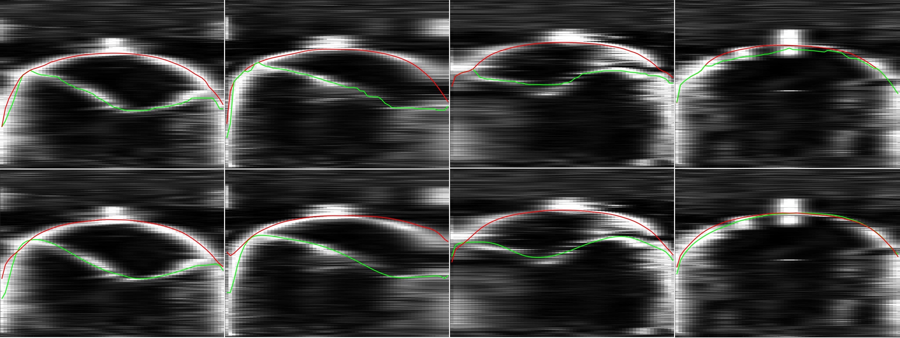

Figure 5: Visualization of sample tomographic images with height $H$ and width $W$. The first row shows the ice-air (red) and ice-bed (green) layers labeled by human annotator, while the second row shows the predicted layers by our model. In general, our predictions not only capture the precise location of each ice layer, but are also smoother than human labels.

3.2 A Multi-task RNN Architecture

The C3D networks discussed above model features both in the temporal and spatial dimensions, but only in very small neighborhoods. For example, they can model the fact that adjacent pixels within the same layer should have similar grayscale value, but not that the layer boundaries themselves (which are usually separated by dozens of pixels at least) are often roughly parallel to one another. Similarly, C3D models some cross-slice constraints but only in a few slices in either direction. We thus also include an RNN that incorporates longer-range cross-slice evidence. Because of the limited training data, we use Gated Recurrent Units (GRUs) [6] since they have fewer learnable parameters than other popular networks like Long Short-Term Memories (LSTMs) [16].

GRU Training and Testing. The multi-task GRU framework is shown in Figure 2. Our model for each individual slice consists of $K$ GRU cells, each responsible for predicting the $k$-th layer in each image. Each GRU cell takes a tomographic slice $I_{d}$ and the output of the previous GRU layer as inputs, and produces $W$ real value numbers indicating the predicted positions of the layer within each column of the image. Each GRU also takes as input the output from the GRU corresponding to the same ice layer in the previous slice, since these layer boundaries should be continuous and roughly smooth. In previous work [8, 23, 35], this prior knowledge was explicitly enforced by pairwise interaction potentials, which were manually tuned by human experts. Here we train RNNs to be able to model more general relationships in a fully learnable way.

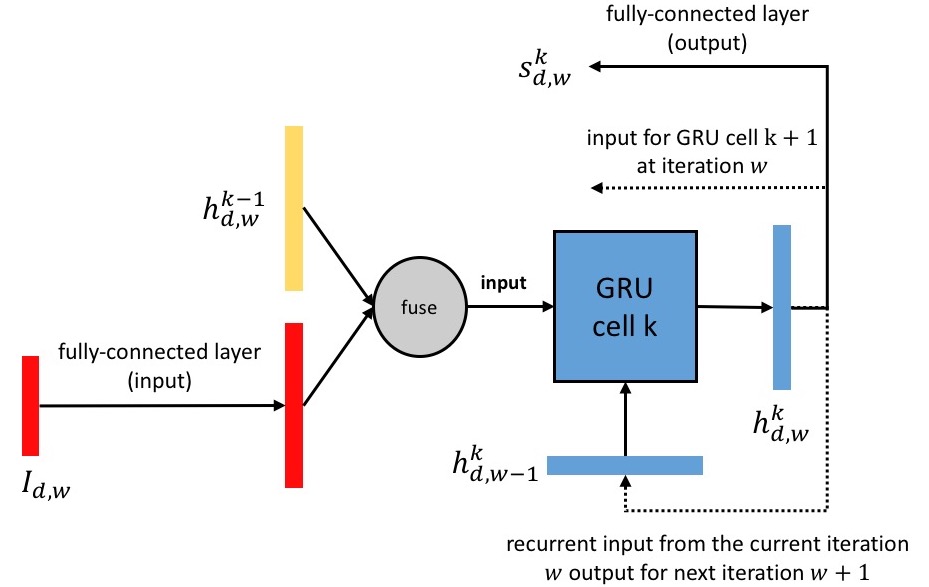
We split each tomographic input image $I_{d}$ into separate column vectors $I_{d,w}$, $w=1,2,\cdots,W$, each with width $1$ and height $H$. Each column vector is projected to the length of the GRU hidden state with a fully-connected layer. During training time, the $k$-th GRU cell is operated for $W$ iterations, where each iteration $w$ predicts the $k$-th layer position in image column $I_{d,w}$. Then in a given iteration $w$, the $k$-th GRU takes the fused features (e.g., using sum or max fusion) of the (resized) image column $I_{d,w}$ and the hidden state $h^{k-1}_{d,w}$ as the input. It also receives the hidden states $h^{k}_{d,w-1}$ of itself in iteration $w-1$ as contextual information. More formally, the $k$-th GRU cell outputs a sequence of hidden states $h^{k}_{d,1},h^{k}_{d,2},\cdots,h^{k}_{d,W}$ with iteration $w=1,2,\cdots,W$, and each hidden state $h^{k}_{d,w}$ is followed by a fully-connected layer to predict the actual layer position $s^{k}_{d,w}$ as shown in Figure 4. Since each GRU has the same operation for each 2D image $I_{d}$, we drop $d$ subscript for simplicity, and compute,

$$\begin{split}&z_{w}=\textrm{sigmoid}(U_{iz}\mathcal{F}(I_{w},h^{k-1}_{w})+U_{hz}h_{w-1}+b_{z}),\\ &r_{w}=\textrm{sigmoid}(U_{iz}\mathcal{F}(I_{w},h^{k-1}_{w})+U_{hz}h_{w-1}+b_{r}),\\ &n_{w}=\textrm{tanh}(U_{in}\mathcal{F}(I_{w},h^{k-1}_{w})+U_{hn}(r_{w}\circ h_{w-1})+b_{n}),\\ &h_{w}=z_{w}\circ h_{w-1}+(1-z_{w})\circ n_{w},\,\textrm{and}\\ &s_{w}=U_{y}h_{w}+b_{y},\end{split}$$

where $\circ$ is the Hadamard product, $z_{w}$, $r_{w}$, $n_{w}$, $h_{w}$, and $s_{w}$ are the reset, input, new gate, hidden state, and output layer position at time $w$, respectively. We use 512 neurons in the hidden layer of the GRU. We train the GRU network with the same L2 Euclidean loss $L_{elu}$ as discussed in the previous section.

Figure 6: Results of the extracted ice-air surfaces based on about 330 tomographic images. The x-axis corresponds to distance along the flight path, the y axis is the width of the tomographic images ($W$), and the color is the height dimension (max height is $H$), which also represents the depth from the radar.

3.3 Combination

We combine our proposed C3D model and GRU model for efficiently encoding spatiotemporal information into explicit structured layer predictions. We use the C3D features $\textrm{C3D}^{k}_{\theta}(I_{d,k})$ (where $\textrm{C3D}^{k}_{\theta}$ denotes the features with model parameters $\theta$ for the $k$-th ice layer) to initialize the $k$-th GRU’s hidden state $h_{1}$, as shown in Figure 2. In the figure, $I_{d}$ is marked in red; this is the frame currently under consideration, which is divided into columns which are then provided to the GRU cells one at a time.

4 Experiments

Figure 7: Sample results of extracted ice-bed surfaces from a sequence of about 330 tomographic images. The x-axis corresponds to distance along the flight path, the y axis is the width of the tomographic images ($W$), and the color is the height dimension (max height is $H$), which also represents the depth from the radar.

	Averaged Mean Error (pixels)	Time (sec)
Xu et al. [35]	11.9	306.0
Ours (C3D + RNN)	10.6	51.6

Table 1: Performance evaluation compared to the state of the art. The accuracy of our approach is computed on the average of the ice-air and ice-bed surfaces and the accuracy of [35] is computed only on the ice-bed surfaces. The running time is measured by processing a sequence of 330 tomographic images.

	Mean Error
	Ice-air surface	Ice-bed surface
Crandall [8]	—	101.6
Lee [23]	—	35.6
Xu et al. (w/o ice mask) [35]	—	30.7
Xu et al. [35]	—	11.9
Ours (RNN)	10.1	21.4
Ours (C2D)	8.8	15.2
Ours (C3D)	9.4	13.9
Ours (C2D + RNN)	8.4	14.3
Ours (C3D + RNN)	8.1	13.1

Table 2: Error in terms of the mean absolute column-wise difference compared to ground truth, in pixels.

4.1 Dataset

We use a dataset of the basal topography of the Canadian Arctic Archipelago (CAA) ice sheets, collected by the Multichannel Coherent Radar Depth Sounder (MCoRDS) instrument [28]. It contains a total of 8 tomographic sequences, each with over 3,300 radar images corresponding to about 50km of flight data per sequence. For training and testing, we also have ground truth that identifies the positions of two layers of interest (the ice-air and ice-bed, i.e., $K=2$). Several examples of these tomographic images and their annotations are shown in Figure 5.

To evaluate our model, we split the data into training and testing sets (60% as training images, 40% as testing images) and learn the model parameters from the training images. More formally, we wish to detect the ice-air and ice-bed layers in each image, then reconstruct their corresponding 3D surfaces from a sequence of tomographic slices. We assume the tomographic sequence has size $C\times D\times H\times W$, where $C$ denotes the number of image channels (which is $1$ for our data), $D$ is the number of slices in the sequence, and $W$ and $H$ are the dimensions of each slice. We also parameterize the output surfaces as sequences, $S^{k}=\{S^{k}_{1},S^{k}_{2},\cdots,S^{k}_{D}\}$, and $S^{k}_{d}=\{s^{k}_{d,1},s^{k}_{d,2},\cdots,s^{k}_{d,W}\}$, where $s^{k}_{d,w}$ indicates the row coordinate of the surface position for column $w$ of slice $d$, and $s^{k}_{d,w}\in[1,H]$ since the boundary can occur anywhere within a column. In our case, $k\in\{0,1\}$ represents the ice-air and ice-bed surfaces, respectively.

Normalization. Since images from different sequences have different sizes (from $824\times 64$ pixels to $2000\times 64$ pixels), we resize all input images to $64\times 64$ by using bicubic interpolation. For each image, we also normalize their pixel values to the interval $[-1,1]$ and subtract the mean value computed from the training images. Further, since the coordinates of the ground truth labels $G^{k}_{d}=\{g^{k}_{d,1},g^{k}_{d,2},\cdots,g^{k}_{d,W}\}$ in each image $I_{d}$ are in absolute coordinates, we follow [30] to normalize them to relative positions in each image. Formally, each ground truth label is normalized as,

$$N(g^{k}_{d,w})=2(g^{k}_{d,w}-H/2)/H,$$ (2)

and we predict the absolute image coordinates $s^{k}_{d,w}$ as,

$$s^{k}_{d,w}=N^{-1}(\textrm{M}_{\theta}(I_{d})),$$ (3)

where $\textrm{M}_{\theta}$ denotes our model with learnable parameters $\theta$.

4.2 Implementation Details

We use PyTorch [1] to implement our model, and do the training and all experiments on a system with Pascal Nvidia Titan X graphics cards. Each tomographic sequence is divided into 10 sub-sequences on average, and we randomly choose $60\%$ of them as training data and the remaining $40\%$ for evaluation. We repeat this training process (each time from scratch) three times and report the average statistics for evaluation.

For C3D training, we use the Adam [21] optimizer to learn the network parameters with batch size of 128, each containing 5 consecutive radar images. The training process is stopped after 20 epochs, starting with a learning rate of $10^{-4}$ and reducing it in half every 5 epochs. The RNN training is applied with the same update rule and batch size, but uses learning rate $10^{-3}$ multiplied by $0.1$ every 10 epochs.

4.3 Evaluation

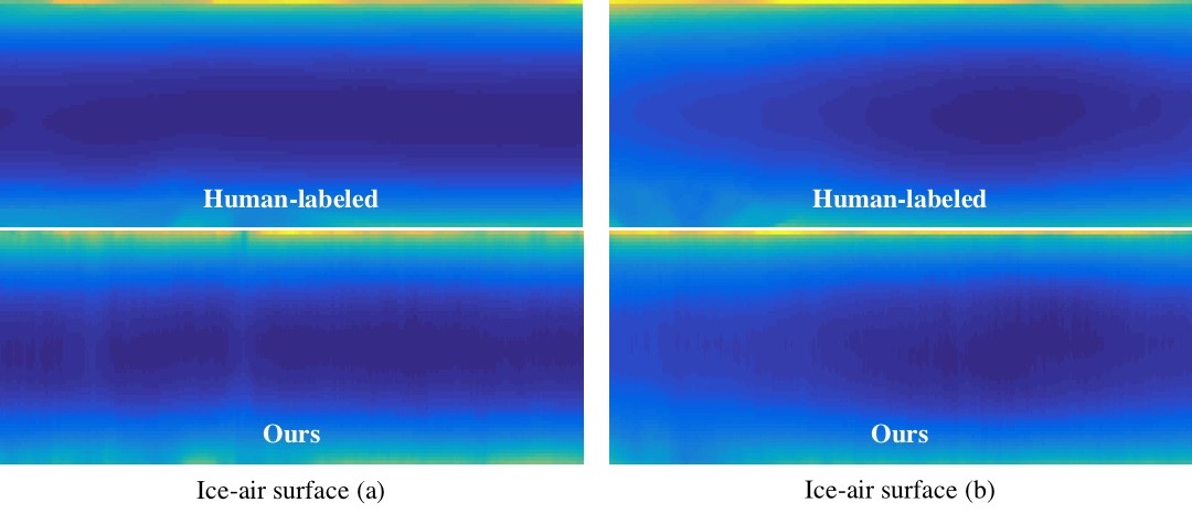
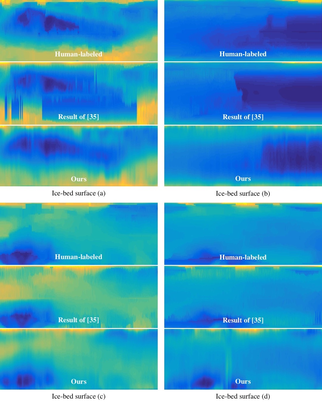
We evaluate our model on estimating the ice-air and ice-bed surfaces from tomographic sequences of noisy radar images. We run inference on the testing sub-sequences and calculate the pixel-level errors with respect to the human-labeled ground truth. We report the results with two summary statistics: mean deviation and running time. As shown in Table 1, the mean error averaged across the two different surfaces is about 10.6 pixels (where the mean ice-air surface error is 8.1 pixels and mean ice-bed surface error is 13.1 pixels), and the running time of processing a topographic sequence with 330 images is about 51.6 seconds. Figure 6 and 7 show some example results of the ice-air and ice-bed surfaces, respectively.

To give some context, we compare our results to previous state of the art techniques as baselines, and results are presented in Table 2. Our first two baselines are Crandall et al. [8], which detects the ice-air and ice-bed layers by incorporating a template model with vertical profile and a smoothness prior into a Hidden Markov Model, and Lee et al. [23], who use Markov-Chain Monte Carlo (MCMC) to sample from the joint distribution over all possible layers conditioned on radar images. These techniques were designed for 2D echogram segmentation and do not include cross-slice constraints, so they perform poorly on this problem. Xu et al. [35] does use information between adjacent images and achieves slightly better results than our technique (11.9 vs 13.1 mean pixel error), but that technique also uses more information. In particular, they incorporate additional non-visual metadata from external sources, such as the “ice mask” which gives prior weak information about anticipated ice thickness (e.g., derived from satellite maps or other prior data). When we removed the ice mask cue from their technique to make the comparison fair, our technique beat theirs by a significant margin (13.1 vs 30.7 mean pixel error). Our approach has two additional advantages: (1) it is able to jointly estimate both the ice-air and ice-bed surfaces simultaneously, so it can incorporate constraints on the similarity of these boundaries, and (2) it requires less than one minute to process an entire sequence of slices, instead of over 5 minutes for [35].

In addition to published methods, we also implemented several baselines to evaluate each component of our deep architecture. Specifically, we implemented: (a) a basic C2D network using the same architecture with the 3D network but with 2D convolution and pooling operations; (b) the RNN network using the extracted features from the C2D as the initial hidden state; (c) the C3D network alone without the RNN; and (d) the RNN network alone without the C3D network. The results of these baselines are also shown in Table 2. The results show that all components of the model are important for achieving good performance, and that the best accuracy is achieved by our full model.

5 Conclusion

We have presented an effective and efficient framework for reconstructing smoothed and structured 3D surfaces from sequences of tomographic images using deep networks. Our approach shows significant improvements over existing techniques: (1) extracts and reconstructs different material boundaries simultaneously; (2) avoids the need for extra evidence from other instruments or human experts; and (3) improves the feasibility of analyzing large-scale datasets by significantly decreasing the running time.

6 Acknowledgments

This work was supported in part by the National Science Foundation (DIBBs 1443054, CAREER IIS-1253549), and used the Romeo cluster, supported by Indiana University and NSF RaPyDLI 1439007. We acknowledge the use of data from CReSIS with support from the University of Kansas and Operation IceBridge (NNX16AH54G). CF was supported by a Paul Purdom Fellowship. We thank Katherine Spoon, as well as the anonymous reviewers, for helpful comments and suggestions on our paper drafts.

References

- [1] http://pytorch.org/.
- [2] J. Andreas, M. Rohrbach, T. Darrell, and D. Klein. Learning to compose neural networks for question answering. arXiv:1601.01705, 2016.
- [3] J. Ba, V. Mnih, and K. Kavukcuoglu. Multiple object recognition with visual attention. arXiv:1412.7755, 2014.
- [4] J. Carreira and A. Zisserman. Quo vadis, action recognition? a new model and the kinetics dataset. arXiv:1705.07750, 2017.
- [5] L. Carrer and L. Bruzzone. Automatic enhancement and detection of layering in radar sounder data based on a local scale hidden Markov model and the Viterbi algorithm. IEEE Transactions on Geoscience and Remote Sensing, pages 962–977, 2017.
- [6] J. Chung, C. Gulcehre, K. Cho, and Y. Bengio. Gated feedback recurrent neural networks. In International Conference on Machine Learning (ICML), 2015.
- [7] J. S. Chung, A. Senior, O. Vinyals, and A. Zisserman. Lip reading sentences in the wild. arXiv:1611.05358, 2016.
- [8] D. J. Crandall, G. C. Fox, and J. D. Paden. Layer-finding in radar echograms using probabilistic graphical models. In International Conference on Pattern Recognition (ICPR), 2012.
- [9] J. Donahue, L. Anne Hendricks, S. Guadarrama, M. Rohrbach, S. Venugopalan, K. Saenko, and T. Darrell. Long-term recurrent convolutional networks for visual recognition and description. In IEEE Conference on Computer Vision and Pattern Recognition (CVPR), 2015.
- [10] J. L. Elman. Finding structure in time. Cognitive science, 14(2):179–211, 1990.
- [11] A. Ferro and L. Bruzzone. A novel approach to the automatic detection of subsurface features in planetary radar sounder signals. In IEEE International Geoscience and Remote Sensing Symposium (IGARSS), 2011.
- [12] A. Ferro and L. Bruzzone. Automatic extraction and analysis of ice layering in radar sounder data. IEEE Transactions on Geoscience and Remote Sensing, pages 1622–1634, 2013.
- [13] G. J. Freeman, A. C. Bovik, and J. W. Holt. Automated detection of near surface martian ice layers in orbital radar data. In Southwest Symposium on Image Analysis & Interpretation (SSIAI), 2010.
- [14] A. Graves. Generating sequences with recurrent neural networks. arXiv:1308.0850, 2013.
- [15] K. Gregor, I. Danihelka, A. Graves, D. J. Rezende, and D. Wierstra. Draw: A recurrent neural network for image generation. arXiv:1502.04623, 2015.
- [16] S. Hochreiter and J. Schmidhuber. Long short-term memory. Neural computation, 9(8):1735–1780, 1997.
- [17] A.-M. Ilisei, A. Ferro, and L. Bruzzone. A technique for the automatic estimation of ice thickness and bedrock properties from radar sounder data acquired at Antarctica. In International Geoscience and Remote Sensing Symposium (IGARSS), 2012.
- [18] A. Karpathy and L. Fei-Fei. Deep visual-semantic alignments for generating image descriptions. arXiv:1412.2306, 2014.
- [19] A. Karpathy, J. Johnson, and L. Fei-Fei. Visualizing and understanding recurrent networks. arXiv:1506.02078, 2015.
- [20] A. Karpathy, G. Toderici, S. Shetty, T. Leung, R. Sukthankar, and L. Fei-Fei. Large-scale video classification with convolutional neural networks. In IEEE Conference on Computer Vision and Pattern Recognition (CVPR), 2014.
- [21] D. Kingma and J. Ba. Adam: A method for stochastic optimization. arXiv:1412.6980, 2014.
- [22] A. Kumar, O. Irsoy, P. Ondruska, M. Iyyer, J. Bradbury, I. Gulrajani, V. Zhong, R. Paulus, and R. Socher. Ask me anything: Dynamic memory networks for natural language processing. In International Conference on Machine Learning, 2016.
- [23] S. Lee, J. Mitchell, D. J. Crandall, and G. C. Fox. Estimating bedrock and surface layer boundaries and confidence intervals in ice sheet radar imagery using MCMC. In International Conference on Image Processing (ICIP), 2014.
- [24] J. A. MacGregor, M. A. Fahnestock, G. A. Catania, J. D. Paden, S. P. Gogineni, S. K. Young, S. C. Rybarski, A. N. Mabrey, B. M. Wagman, and M. Morlighem. Radiostratigraphy and age structure of the greenland ice sheet. Journal of Geophysical Research, 2015.
- [25] J. E. Mitchell, D. J. Crandall, G. C. Fox, and J. D. Paden. A semi-automatic approach for estimating near surface internal layers from snow radar imagery. In International Geoscience and Remote Sensing Symposium (IGARSS), 2013.
- [26] C. Panton. Automated mapping of local layer slope and tracing of internal layers in radio echograms. Annals of Glaciology, 55(67):71–77, 2014.
- [27] A. Piergiovanni, C. Fan, and M. S. Ryoo. Learning latent sub-events in activity videos using temporal attention filters. In AAAI Conference on Artificial Intelligence, 2017.
- [28] F. Rodriguez-Morales, S. Gogineni, C. J. Leuschen, J. D. Paden, J. Li, C. C. Lewis, B. Panzer, D. G.-G. Alvestegui, A. Patel, K. Byers, et al. Advanced multifrequency radar instrumentation for polar research. IEEE Transactions on Geoscience and Remote Sensing, 2014.
- [29] K. Simonyan and A. Zisserman. Very deep convolutional networks for large-scale image recognition. arXiv:1409.1556, 2014.
- [30] A. Toshev and C. Szegedy. Deeppose: Human pose estimation via deep neural networks. In IEEE Conference on Computer Vision and Pattern Recognition (CVPR), 2014.
- [31] D. Tran, L. Bourdev, R. Fergus, L. Torresani, and M. Paluri. Learning spatiotemporal features with 3d convolutional networks. In International Conference on Computer Vision (ICCV), 2015.
- [32] K.-L. Tseng, Y.-L. Lin, W. Hsu, and C.-Y. Huang. Joint sequence learning and cross-modality convolution for 3d biomedical segmentation. arXiv:1704.07754, 2017.
- [33] O. Vinyals, A. Toshev, S. Bengio, and D. Erhan. Show and tell: A neural image caption generator. arXiv:1411.4555, 2014.
- [34] J. Weston, A. Bordes, S. Chopra, A. M. Rush, B. van Merriënboer, A. Joulin, and T. Mikolov. Towards ai-complete question answering: A set of prerequisite toy tasks. arXiv:1502.05698, 2015.
- [35] M. Xu, D. J. Crandall, G. C. Fox, and J. D. Paden. Automatic estimation of ice bottom surfaces from radar imagery. arXiv:1712.07758, 2017.
- [36] L. Yu, W. Zhang, J. Wang, and Y. Yu. Seqgan: Sequence generative adversarial nets with policy gradient. In AAAI Conference on Artificial Intelligence, 2017.
- [37] J. Yue-Hei Ng, M. Hausknecht, S. Vijayanarasimhan, O. Vinyals, R. Monga, and G. Toderici. Beyond short snippets: Deep networks for video classification. In IEEE conference on computer vision and pattern recognition (CVPR), 2015.