Full-sky ray-tracing simulation of weak lensing using ELUCID simulations:
exploring galaxy intrinsic alignment and cosmic shear correlations

Abstract

The intrinsic alignment of galaxies is an important systematic effect in weak-lensing surveys, which can affect the derived cosmological parameters. One direct way to distinguish different alignment models and quantify their effects on the measurement is to produce mocked weak-lensing surveys. In this work, we use full-sky ray-tracing technique to produce mock images of galaxies from the ELUCID $N$-body simulation run with the WMAP9 cosmology. In our model we assume that the shape of central elliptical galaxy follows that of the dark matter halo, and spiral galaxy follows the halo spin. Using the mocked galaxy images, a combination of galaxy intrinsic shape and the gravitational shear, we compare the predicted tomographic shear correlations to the results of KiDS and DLS. It is found that our predictions stay between the KiDS and DLS results. We rule out a model in which the satellite galaxies are radially aligned with the center galaxy, otherwise the shear-correlations on small scales are too high. Most important, we find that although the intrinsic alignment of spiral galaxies is very weak, they induce a positive correlation between the gravitational shear signal and the intrinsic galaxy orientation (GI). This is because the spiral galaxy is tangentially aligned with the nearby large-scale overdensity, contrary to the radial alignment of elliptical galaxy. Our results explain the origin of detected positive GI term from the weak-lensing surveys. We conclude that in future analysis, the GI model must include the dependence on galaxy types in more detail.

1 Introduction

In the context of General Relativity, photos emitted from distant galaxies are continuously deflected by the intervening mass field of the large-scale structures (Schneider et al., 1992; Meylan et al., 2006; Bartelmann & Maturi, 2016). This gravitational lensing effect, referred to as “cosmic shear", produces some coherent distortions of the observed galaxy images, which can be measured to probe the matter distribution in the universe (Mellier, 1999; Van Waerbeke et al., 2001; Kilbinger, 2003; Fu et al., 2008; Kilbinger, 2015; Foreman et al., 2016). Great progress has been made in using cosmic shears to constrain cosmological models (see Kilbinger 2015 for a review), to estimate the dark energy parameter $w$ (Bridle & King, 2007; Levy & Brustein, 2009; Battye et al., 2015), and to test theories of modified gravity (Ling et al., 2015; Higuchi & Shirasaki, 2016).

Observational results from recent weak-lensing surveys, such as Canada-France-Hawaii Telescope Lensing Survey (CFHTLenS, Heymans et al., 2012, 2013) and Deep Lens Survey (DLS, Jee et al., 2013, 2016a, 2016b), demonstrate that cosmic shears can be combined with other observations, such as the cosmic microwave background (CMB), baryon acoustic oscillations (BAO), and galaxy cluster abundance, to break the degeneracy among different cosmological parameters (e.g., $\Omega_{\rm m}$-$\sigma_{8}$). Thus, accurate measurement of weak lensing effects has been one of the main goals of many ongoing and upcoming galaxy surveys, such as the Kilo-Degree Survey (KiDS, de Jong et al., 2015), Dark Energy Survey (DES, Dark Energy Survey Collaboration et al., 2016), Hyper Suprime-Cam Survey (HSC, Miyazaki et al., 2012), Euclid (Laureijs et al., 2011) and the Large Synoptic Survey Telescope (LSST, LSST Science Collaboration et al., 2009).

These surveys will provide high-quality data with very wide sky coverages, and the statistical uncertainties in weak lensing measurements are expected to be small. However, high accuracy analyses of cosmic shear also requires understanding the systematics in the data, such as those in measurements of galaxy ellipticity and the point spread function. In addition, accurate theoretical modeling is also necessary in order to interpret the observed data.

One of the most serious astrophysical systematic effects in the era of accurate weak-lensing analyses is the intrinsic alignment (IA) of galaxies (Heavens et al. 2000; Crittenden et al. 2001; Jing 2002; see Kirk et al. 2015; Troxel & Ishak 2015 for a review), which can mimic the gravitational lensing signal, thereby contaminating the measurements of cosmic shears. A significant signal of intrinsic alignments has been detected by Mandelbaum et al. (2006) in the luminous red galaxies from the Sloan Digital Sky Survey (SDSS, York et al., 2000), and the authors concluded that neglecting such alignments can lead to an underestimate of the linear amplitude of density fluctuations by $20\%$ for cosmic shear surveys at $z\sim 1$. Clearly, an accurate model for galaxy IA, which is capable of describing its dependence on redshift and galaxy properties, is crucial for maximizing the science returns of ongoing and future weak lensing surveys (Krause et al., 2016).

There have been numerous investigations on galaxy IA. Based on the tidal field theory (Catelan et al., 2001), Hirata & Seljak (2004) developed a linear model for galaxy IA, which was later improved to include some non-linear effects (Bridle & King, 2007; Blazek et al., 2012). A useful formula with a single parameter was introduced by Joachimi et al. (2011), which can easily be included in the analyses of cosmic shears from observational data (Kirk et al., 2010; Heymans et al., 2013; Jee et al., 2016a; Hildebrandt et al., 2017; Joudaki et al., 2017). As a more accurate description of galaxy IA, a halo model is developed (Schneider & Bridle, 2010), which can predict the IA signal as a function of galaxy properties. However, as pointed in Joachimi et al. (2013a), most of these simple IA models are expected to work only at low $z$, and it is still unclear how galaxy IA varies as a function of galaxy properties at high $z$.

$N$-body and Hydro-dynamical simulations are also extensively used to study galaxy IA. When $N$-body simulations are used for the purpose, assumptions about the connection between galaxy shape and dark matter halo shape have to be made. Kang et al. (2007) used $N$-body simulations to explain the observed small-scale alignment of satellites galaxies around central galaxies in the SDSS data (Yang et al., 2006). They found that the orientations of elliptical galaxies follow that of the host halos, albeit with some mis-alignment, and that the spins of spiral galaxies follow that of their host halos. This assumption is later confirmed (e.g., Faltenbacher et al., 2009; Okumura et al., 2009; Agustsson & Brainerd, 2010). With similar assumptions about how galaxies are aligned with dark matter halos, Joachimi et al. (2013b) measured galaxy IA on large scales from the Millennium Simulations (Springel et al., 2005) and found that early-type galaxies are strongly aligned with each other, but spiral galaxies do not show significant correlation signals between their intrinsic ellipticities. This dependence on galaxy-type agrees with observational results. (e.g., Joachimi et al., 2011; Heymans et al., 2013; Mandelbaum et al., 2011). More recently, cosmological hydrodynamical simulations have been used to predict the galaxy IA (e.g., Dong et al., 2014; Tenneti et al., 2014; Chisari et al., 2015, 2016, 2017; Velliscig et al., 2015; Hilbert et al., 2017; Tenneti et al., 2016). The main merit of using a hydro-dynamical simulation is that galaxy shapes are directly predicted by the simulation. In agreement with previous analytical models and $N$-body simulations, these hydro-dynamical simulations also indicate that elliptical galaxies have a stronger tendency to align with each other on large scales than do spiral galaxies. However, due to limited volumes of these simulations (often around 100Mpc/$h$) and different treatment of baryonic physics, the predicted galaxy IA signal and its dependence on galaxy properties and redshift still varies from simulation to simulation.

Although an accurate model for galaxy IA is still not available at the present, the main assumption, adopted in $N$-body simulations, that elliptical galaxies follow the shapes, while spirals follow the spins, of host halos (e.g., Joachimi et al., 2013b), can be checked by comparing real and mocked observational data of galaxy shear correlations. This can be achieved by using ray tracing in an $N$-body simulation combined with a model of galaxy formation which can predict galaxy shapes, luminosities and positions. With such an approach, we can produce observable images of galaxies and obtain the auto- and cross-correlation functions between gravitational shear and galaxy intrinsic ellipticity at different redshifts. We can then compare model predictions with results obtained from two recent surveys, KiDS and DLS, and examine the importance of galaxy IA. The results of these two surveys show a $\sim 2\sigma$ tension in $S_{8}\equiv\sigma_{8}\sqrt{\Omega_{\rm m}/0.3}$, with KiDS giving $S_{8}=0.745\pm 0.039$ and DLS giving $0.818_{-0.026}^{+0.034}$. The main goal of this paper is to use such approach to constrain galaxy IA models and to examine the contamination from IA in the 2-point correlation functions of the cosmic shear.

As a ‘standard’ algorithm, the multiple-plane ray-tracing simulation with the flat-sky approximation (e.g., Jain et al., 2000; White & Vale, 2004; Hilbert et al., 2009) has been widely used to simulate lensing maps for small-field survey. It also roughly works for hundreds of square degree surveys, such as KiDS with 450 square degrees (hereafter KiDS-450, Hildebrandt et al., 2017), but will not suitable for even large-filed surveys such as Euclid and LSST (Kitching et al., 2016; Kilbinger et al., 2017; Lemos et al., 2017). To quantify the effect of cosmic variance in the small-field surveys, one needs construct a lot of light cones to simulated different realizations. In this paper, we adopt ray-tracing code on a curved sky to simplify this procedure and to prepare for these large-field surveys.

Full-sky weak-lensing maps have already been constructed in a number of papers (Teyssier et al., 2009; Becker, 2013; Fosalba et al., 2008, 2015; Shirasaki et al., 2015). These simulations usually cover a sufficiently large volume to compute a full-sky convergence (and shear) maps, and explore the lensing power at both the linear and nonlinear regimes. In this paper, we follow the ray-tracing method of Das & Bode (2008); Teyssier et al. (2009); Becker (2013). We perform high resolution (both in space and in mass) lensing simulations, using an iterative scheme of spherical harmonic analysis, to model lensed properties of ’semi-analytic’ galaxies in the simulation. These simulated galaxies allow us to study the statistical properties of galaxy alignments, and to compare our mock observations with the observational results from both DLS (Jee et al., 2016a, b) and KiDS-450 (Hildebrandt et al., 2017) using tomographic correlation functions.

The paper is organized as follows. In Section 2 we first summarize the basic theoretical background of weak lensing, focusing on the power spectrum and shear correlation analyses. In Section 3 we introduce the simulations and the spherical ray-tracing technique. Section 4 describes how we model galaxy properties, such as luminosity, morphology and shape, from the semi-analytic model, and we also present results of intrinsic alignments of galaxies and their dependence on galaxy type and halo mass. In Section 5, we describe the tomographic analyses of cosmic shears in our lensing simulation, compare model predictions with observational data, and quantify the contributions of the intrinsic-intrinsic (II) shear correlation and the gravitational shear-intrinsic (GI) shear correlation by spiral and elliptical galaxies. Conclusions and discussions are given in Section 6.

2 COSMOLOGICAL WEAK LENSING

In this section, we briefly summarize the theoretical background for the analyses of weak gravitational lensing and describe some basics about intrinsic alignment and shear correlations.

2.1 Basics

In general, for a source galaxy with the observed angular position $\bm{\theta}$ and its real position $\bm{\beta}$, one can characterize the deformation effect of cosmic shear through the distortion matrix (Schneider et al., 1992; Jain et al., 2000),

$$\mathcal{A}(\bm{\theta})=\frac{\partial\bm{\beta}}{\partial\bm{\theta}}\equiv\begin{pmatrix}1-\kappa-\gamma_{1}&-\gamma_{2}-\omega\\ -\gamma_{2}+\omega&1-\kappa+\gamma_{1}\end{pmatrix},$$ (1)

where $\kappa$ is the convergence, $\bm{\gamma}=\gamma_{1}+{\rm i}\gamma_{2}$ defines the complex shear in lensing, and the additional antisymmetric quantity, $\omega$, describes an overall rotation in the lensed images. In the weak lensing regime (i.e., $\kappa,\bm{\gamma}\ll 1$) and to the linear order, the components of the matrix are related to the second derivatives of the gravitational potential as (Bartelmann & Schneider, 2001; Hilbert et al., 2009; Kilbinger, 2015)

$$\mathcal{A}_{ij}(\bm{\theta},\chi)=\delta_{ij}-\frac{2}{c^{2}}\int_{0}^{\chi}{\rm d}\chi^{\prime}\frac{r(\chi-\chi^{\prime})r(\chi^{\prime})}{r(\chi)}\Phi_{,ij}(r(\chi^{\prime})\bm{\theta},\chi^{\prime}),$$ (2)

where $\delta_{ij}$ is the Kronecker delta, $c$ is the speed of light, $\chi$ is the comoving distance and $r(\chi)$ the comoving angular diameter distance. According to the Poisson equation, gravitational potential $\Phi$ can be related to the density contrast $\delta$. Hence, convergence $\kappa$ can be expressed as a weighted integral of the over-density $\delta$ along the line of sight,

$$\kappa(\bm{\theta},\chi)=\frac{3H_{0}^{2}\Omega_{{\rm m}}}{2c^{2}}\int_{0}^{\chi}{\rm d}\chi^{\prime}\frac{r(\chi-\chi^{\prime})r(\chi^{\prime})}{r(\chi)}\frac{\delta(r(\chi^{\prime})\bm{\theta},\chi^{\prime})}{a(\chi^{\prime})},$$ (3)

where $H_{0}$ is the Hubble constant, $\Omega_{{\rm m}}$ is the matter density in units of the critical density, and $a(\chi^{\prime})$ is the scale factor at $\chi^{\prime}$.

2.2 Power Spectrum of Weak Lensing Field

In the flat-sky limit, the power spectrum of the convergence $C^{\kappa\kappa}(\ell)$ on the modulus $\ell$ is known as the two-point correlation in Fourier space,

$$\langle\tilde{\kappa}(\bm{\ell})\tilde{\kappa}^{*}(\bm{\ell}^{\prime})\rangle=(2\pi)^{2}\delta_{\rm D}(\bm{\ell}-\bm{\ell}^{\prime})C^{\kappa\kappa}(\ell),$$ (4)

where $\delta_{\rm D}(\bm{\ell})$ is the Dirac delta function. Using equation (3), one can derive the angular power spectrum of the convergence field in the Limber approximation,

$$C^{\kappa\kappa}(\ell)=\int^{\chi_{\rm H}}_{0}{\rm d}\chi\frac{W(\chi)^{2}}{r(\chi)^{2}}P_{\delta}\left(k=\frac{\ell}{r(\chi)},\chi\right),$$ (5)

where $P_{\delta}(k,\chi)$ is the 3-D power spectrum of the matter distribution at the given comoving distance $\chi$, and the integral is calculated along the line of sight to the comoving horizon distance $\chi_{\rm H}$. Here the weight function $W(\chi)$ is defined as,

$$W(\chi)=\frac{3H_{0}^{2}\Omega_{{\rm m}}}{2c^{2}}\frac{r(\chi_{\rm H}-\chi)r(\chi)}{r(\chi_{\rm H})}\frac{1}{a(\chi)}.$$ (6)

From the non-linear theoretical models, such as the Halofit model (Smith et al., 2003; Takahashi et al., 2012), one can predict the convergence power spectrum $C^{\kappa\kappa}(\ell)$ from the non-linear $P_{\delta}(k)$. Therefore, the weak lensing survey can be used to probe the gravitational growth of the density structure.

While dealing with full-sky measurements, it is useful to note that the angular power spectrum of weak lensing convergence $\kappa$ and complex shear $\bm{\gamma}$ can be derived from the spin-$s$ spherical harmonics ${}_{s}Y_{\ell}^{m}$ (Stebbins, 1996). The relations of power spectra between the convergence, shear E- and B-mode (Schneider et al., 2002; Bunn, 2003; Bunn et al., 2003; Zhao & Baskaran, 2010) have been derived by Hu (2000) for an all-sky lensing deformation tensor field. Here we briefly summarize the spin-$s$ spherical harmonic decomposition of the full-sky lensing, referring the reader to Hu (2000) for detailed discussions of the power spectrum in weak lensing.

As reviewed in the appendix of Becker (2013), the convergence, lensing shear and rotation in the distortion matrix (Eq. 1) can be decomposed by the spherical harmonics (Hu, 2000; Becker, 2013),

$$\kappa(\hat{\bm{n}})=-\frac{1}{2}\sum_{\ell m}\ell(\ell+1)\phi_{\ell m}Y_{\ell}^{m}(\hat{\bm{n}})$$ (7)

$$\gamma_{1}(\hat{\bm{n}})\pm i\gamma_{2}(\hat{\bm{n}})=\frac{1}{2}\sum_{\ell m}\sqrt{\frac{(\ell+2)!}{(\ell-2)!}}(\phi_{\ell m}\pm i\Omega_{\ell m})_{\pm 2}Y_{\ell}^{m}(\hat{\bm{n}})$$ (8)

$$\omega(\hat{\bm{n}})=-\frac{1}{2}\sum_{\ell m}\ell(\ell+1)\Omega_{\ell m}Y_{\ell}^{m}(\hat{\bm{n}}),$$ (9)

where $\phi$ is the lensing deflection potential, $\Omega$ is the pseudo-scalar potential (as described by Stebbins, 1996), and $\hat{\bm{n}}$ denotes a given position on the sky. Consequently, the different power spectra can be related as,

$$C^{\kappa\kappa}(\ell)=\frac{1}{4}\ell^{2}(\ell+1)^{2}C^{\phi\phi}(\ell)$$ (10)

$$C^{\omega\omega}(\ell)=\frac{1}{4}\ell^{2}(\ell+1)^{2}C^{\Omega\Omega}(\ell)$$ (11)

$$C^{EE}(\ell)=\frac{1}{\ell^{2}(\ell+1)^{2}}\frac{(\ell+2)!}{(\ell-2)!}C^{\kappa\kappa}(\ell)$$ (12)

$$C^{BB}(\ell)=\frac{1}{\ell^{2}(\ell+1)^{2}}\frac{(\ell+2)!}{(\ell-2)!}C^{\omega\omega}(\ell).$$ (13)

Thus in the flat-sky limit, one has $\frac{1}{\ell^{2}(\ell+1)^{2}}\frac{(\ell+2)!}{(\ell-2)!}\approx 1$, showing that $C^{EE}(\ell)$ equals $C^{\kappa\kappa}(\ell)$ at small scales (Kitching et al., 2016; Kilbinger et al., 2017).

2.3 Cosmic Shear and Intrinsic Alignment

Weak lensing will induce an additional coherent deformation to the intrinsic galaxy shape, which means that the measured ellipticity $\bm{\epsilon}^{({\rm obs})}$ of a galaxy can be expressed as (Bartelmann & Schneider, 2001; Meylan et al., 2006),

$$\bm{\epsilon}^{({\rm obs})}=\bm{g}+\bm{\epsilon}^{({\rm I})}+\bm{\epsilon}^{({\rm rnd})},$$ (14)

where $\bm{g}$ is the reduced shear, defined as $\bm{g}=\bm{\gamma}/(1-\kappa)$, and $\bm{\epsilon}^{({\rm rnd})}$ denotes the noise part in galaxy shape measurements, which is assumed to be uncorrelated with the other components. In the weak lensing regime, $\kappa$ is small and the $\bm{\gamma}\simeq\bm{g}$ assumption is often made. The intrinsic shape of a galaxy is described as $\bm{\epsilon}^{({\rm I})}$. Ideally, if the intrinsic ellipticities of galaxies are isotropic, the lensing shear $\bm{g}$ can be derived by averaging over a population of galaxies. However, it is not the case for real data, because of the presence of correlated intrinsic alignment of observed galaxies.

The observed 2-point shear correlation function consists of the following contributions (Troxel & Ishak, 2015; Jee et al., 2016a; Krause et al., 2016),

$$\langle\bm{\epsilon}^{({\rm obs})}_{i}\bm{\epsilon}^{({\rm obs})}_{j}\rangle=\langle\bm{g}_{i}\bm{g}_{j}\rangle+\langle\bm{\epsilon}^{({\rm I})}_{i}\bm{g}_{j}\rangle+\langle\bm{\epsilon}^{({\rm I})}_{i}\bm{\epsilon}^{({\rm I})}_{j}\rangle,$$ (15)

where we assume that the two observed galaxies are located at the redshifts $z_{i}$ and $z_{j}$ (with $z_{i}\leqslant z_{j}$), respectively. The first term, $\langle\bm{g}_{i}\bm{g}_{j}\rangle$, represents the shear-shear correlation, GG, which is the weak lensing signal we want to extract. The correlation $\langle\bm{\epsilon}^{({\rm I})}_{i}\bm{g}_{j}\rangle$ , often named as GI, is the cross term between gravitational shear and intrinsic ellipticity. This correlation comes from the fact that the shape of a distant galaxy ‘$j$’ is lensed by the foreground gravitational potential, in which galaxy ‘$i$’ is intrinsically aligned with the underlying tidal field (Hirata & Seljak, 2004). Since nearby galaxies are affected by the same environment, the intrinsic-intrinsic correlation $\langle\bm{\epsilon}^{({\rm I})}_{i}\bm{\epsilon}^{({\rm I})}_{j}\rangle$, often referred as II term, may be non-zero. Both the II and GI correlations can contaminate our measurements of cosmic shear, and are important to quantify, particularly in accurate shear measurements expected from future large lensing surveys (Krause et al., 2016).

In order to model the II and GI parts in the measurements, Hirata & Seljak (2004), Bridle & King (2007) and Joachimi et al. (2011) developed a non-linear intrinsic alignment model based on the work of Catelan & Porciani (2001). In this model, the power spectra of the II and GI contributions are related to the non-linear matter power spectrum as $P_{\rm II}(k,z)=f^{2}(z)P_{\delta}(k,z)$ and $P_{\rm GI}(k,z)=f(z)P_{\delta}(k,z)$, respectively. Here the modification factor $f(z)$ is defined as

$$f(z)=-A_{\rm IA}C_{1}\rho_{\rm c}\frac{\Omega_{\rm m}}{D(z)}\left(\frac{1+z}{1+z_{0}}\right)^{\eta}\left(\frac{L}{L_{0}}\right)^{\beta},$$ (16)

where $A_{\rm IA}$ is a free parameter; $C_{1}=5\times 10^{-14}h^{-2}{\rm M}_{\sun}^{-1}{\rm Mpc}^{3}$; $\rho_{c}$ is the critical density at the present; and $D(z)$ is the linear growth factor (normalized to unity at $z=0$). The free parameters $\eta$ and $\beta$ account for the dependence on redshift and luminosity around the pivot redshift $z_{0}$ and luminosity $L_{0}$. Following the discussion of Joudaki et al. (2017) based on the CFHTLenS data, we fix $\eta=0$ and $\beta=0$ in our model fitting. These formulas are used in section 5.3.2 to fit the measurements of GI and II terms from our simulation. There we will see that the sign of $A_{\rm IA}$ actually depends on galaxy type.

3 Numerical simulations

In this section, we describe the $N$-body simulations (3.1), the spherical ray-tracing technique (3.2), and the comparison between the measured power spectra from our lensing simulations and those from the non-linear model predictions.

3.1 $N$-body Simulation

Table 1: The parameters of the two $N$-body simulations. Cosmological parameters are given as $\Omega_{{\rm m}},\Omega_{\Lambda}$, $h$ and $\sigma_{8}$. $L_{{\rm box}}$ is the box-size, $m_{{\rm p}}$ is the particle mass, $l_{{\rm soft}}$ is the softening length.

Simulation	$\Omega_{{\rm m}}$	$\Omega_{\Lambda}$	$h$	$\sigma_{8}$	$L_{{\rm box}}/h^{-1}{\rm Mpc}$	$m_{{\rm p}}/(10^{10}h^{-1}{\rm M}_{\sun})$	$l_{{\rm soft}}/h^{-1}{\rm kpc}$
PS-I	0.260	0.740	0.710	0.80	1000	0.249	7.0
L500	0.282	0.718	0.697	0.82	500	0.034	3.5

We use two sets of different $N$-body cosmological simulations. The first one is a part of the ELUCID project (Wang et al., 2014, 2016; Li et al., 2016; Tweed et al., 2017), which is run with $3072^{3}$ dark matter particles in a cubic box with $L_{{\rm box}}=500h^{-1}{\rm Mpc}$ on each side. This simulation is referred as L500 in the following. The cosmological parameters of L500 are from the WMAP9 cosmology (Hinshaw et al., 2013). The second simulation is the Pangu simulation (PS-I), performed by the Computational Cosmology Consortium of China (Li et al., 2012), which has the same number of particles as L500, but with a box size of $1000h^{-1}{\rm Mpc}$ on each side. The cosmological parameters of PS-I are from the WMAP7 (Komatsu et al., 2011). In Table. 1, we list the parameters of the two $N$-body simulations. Both simulations were run using the GADGET-2 code (Springel, 2005).

With its higher mass resolution, the L500 simulation is used to generate galaxies from a semi-analytical model (Luo et al., 2016). This model is based on the L-Galaxies model developed by the Munich group (e.g., Guo et al., 2013) (see Section 4.1 for more details). We do not produce mock galaxies using the PS-I simulation due to its lower mass resolution, but use it as a reference to check our calculation of the convergence power spectrum on large scales.

3.2 Spherical Ray-tracing Simulation

To perform a ray-tracing simulation with full-sky coverage, we follow the multi-plane algorithm developed by Das & Bode (2008), Teyssier et al. (2009), and Becker (2013). In order to control the residual in the solution of the lensing potential, we implement an iterative spherical harmonic analysis scheme, which is different from the multi-grid method adopted by Becker (2013). In the following, we briefly summarize the main procedures; more details can be found in Appendix A.

To trace the trajectory of a light beam, we first employ the $N$-body simulations to build light-cone to redshift $z_{{\rm max}}\sim 2.0$. In practice the simulation boxes are divided into sets of small cubic boxes with $\sim 100h^{-1}{\rm Mpc}$ on each side. These cell boxes are appropriately piled together so as to cover the past light-cone from $z=0$ to $z=z_{{\rm max}}$. For both L500 and PS-I described above, a full-sky light-cone can be constructed in this manner. Note that the size of our simulation box is relatively small compared with the comoving distance to redshift $z_{\rm s}=2.0$ and periodic effects will show up at several specific directions, especially along the box axes, but the effects disappear very quickly apart from these directions.

Then each light-cone is divided into a set of spherical shells with a thickness of $50h^{-1}\rm Mpc$ centered at the observer, and the dark matter distribution in the corresponding shells is projected into pixels defined by the HEALPix tessellation (Górski et al., 2005; Calabretta & Roukema, 2007). The HEALPix resolution parameter is set to $N_{{\rm side}}=8192$, which gives an angular resolution of $\sim 0.43$ arcmin. The projected surface mass densities are calculated for each shell using the SPH algorithm (Li et al., 2005; Springel, 2010). We use the nearest 64 particles to define the kernel size, but keep the smoothing length larger than two HEALPix cells in high-density regions. The lensing potential for the $n$-th shell, $\phi^{(n)}_{\ell m}$, is then obtained, using the Poisson equation, from the mass density shell after applying an iterative spherical harmonic transformations (refer to as HEALPix predefined functions),

$$-\ell(\ell+1)\phi^{(n)}_{\ell m}=2\kappa^{(n)}_{\ell m}.$$ (17)

To perform multi-sphere ray-tracing simulations, we set the initial positions of ray-beams at the centers of the HEALPix cells, and propagate light rays from the observer to a desired redshift applying deflection angle,

$$\alpha^{(n)}_{\ell m}=-\sqrt{\ell(\ell+1)}\phi^{(n)}_{\ell m}.$$ (18)

Figure 1: One realization of the convergence map from PS-I light-cone for sources at $z_{\rm s}=1.0$.

Figure 2: Comparison between the power spectrum from ray tracing with the model predictions. The top panels show the angular power spectrum of convergence (red solid line), shear E-mode (blue) and B-mode (magenta), and rotation (cyan) for sources at $z_{s}=1$ from the PS-I (left panel) and L500 (right panel). The measured convergence power from the Born approximation (grey dashed line) and revised Halofit model (Takahashi et al., 2012) predictions (black dashed line) are also shown for comparison. The relative deviations of the measured convergence statistics and from predictions are presented in the middle panels. Lower panels show the ratios of the E- and B-modes with to the convergence and rotation modes, respectively.

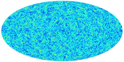
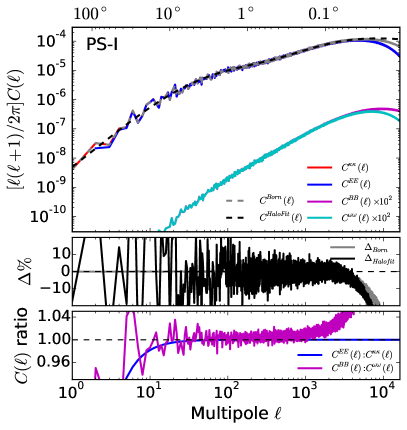
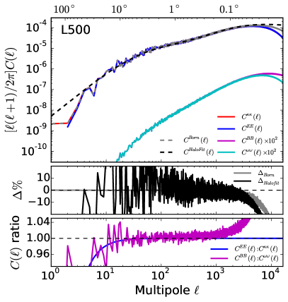
From our lensing simulation, we evaluate the distortion matrix $\mathcal{A}$ on each lensing shell and construct the full-sky map of the convergence and lensing shear. As an illustration, Fig. 1 shows one realization of our simulated full-sky convergence map, $\kappa$, for sources at redshift $z_{s}=1.0$. In Fig. 2, we show the power spectra measured from PS-I (left panels) and L500 simulation (right panels). The top panels show the angular power spectra of the convergence (red solid line), the shear E-mode (blue) and B-mode (magenta), and the rotation mode (cyan). We also show the prediction from the Born approximation (Cooray & Hu, 2002) by stacking density field along the line-of-sight in our mock light-cone as the grey dashed line and the theoretical prediction from the revised non-linear Halofit (Takahashi et al., 2012; Peacock & Smith, 2014) as the black dashed line. The middle panels of Fig. 2 show the relative deviations between convergence powers measured from our ray-tracing simulation and the theoretical predictions, like that the relative deviation between the ray-tracing simulation and Halofit model is defined by $\Delta_{\rm Halofit}=\left[C^{\kappa\kappa}(\ell)-C^{\rm Halofit}(\ell)\right]/C^{\rm Halofit}(\ell)$.

The measured convergence power from our ray-tracing simulation agrees well with the theoretical prediction of Halofit, and the relative error is less than 10 per cent at $\ell\lesssim 4000$. At large scales, $\ell\lesssim 10$, the power from the PS-I simulation is in better agreement with theoretical predictions than the L500 simulation, as is expected from the fact that PS-I has a larger box to represent the matter power on large scales. The prediction from Born approximation is closer to that of Halofit at small scales than our ray-tracing simulation, because both Born approximation and Halofit are based on the first-order approximations. This good agreement, within 10 per cent for $\ell\lesssim 6000$, roughly on scales larger than the smoothing scale in our simulation, indicates that the revised Halofit model (Takahashi et al., 2012) provides a good approximation to the non-linear matter power spectrum. In addition, since the power spectra from our Born approximation and full-sky ray-tracing simulation are both based on the same convergence $\kappa$ maps, the difference between the two is not caused by the smoothing effect. The grey lines in the middle panels of Fig. 2 show that Born approximation can cause a deviation of more than 10 per cent for $\ell>6000$.

The bottom panels show the ratio of shear E-mode and B-mode power spectra relative to the measured convergence and rotation mode spectra, respectively. As shown in Section 2.2, at high-$\ell$ (small scales), one has $C^{EE}(\ell)=C^{\kappa\kappa}(\ell)$ from the full-sky weak lensing. Our corresponding measurements on small scales are indeed in consistent with this expectation. At large scales (low-$\ell$), we must take account of the extra factor of $(\ell-1)(\ell+2)/\ell/(\ell+1)$ to explain the difference between the power spectrum of the shear E-mode and convergence spectrum. As discussed in Becker (2013), we also measure the power spectra of the B-mode and the rotation mode from our lensing simulation. We find that the B-mode power is effectively suppressed relative to the E-mode by more than four orders of magnitude. Moreover, the power ratio between the B-mode and the rotation mode shows that the extra numerical B-mode in our simulation is negligible, and the accuracy of our shear map is only limited by the smoothing length at small scales. We refer the reader to Fig. 13 in Appendix A for more details. Compared with the Becker (2013) results, the predictions of our simulations for the convergence and shear power spectra are more accurate extending to higher $\ell$.

4 GALAXY MODELING

One important merit of our work is to include model galaxies in the N-body simulations and to predict shear correlation functions that can be compared directly to observations. In this section, we describe how we model the physical properties of galaxies and show the intrinsic alignment of the model galaxies.

4.1 Semi-analytic Models

Figure 3: Cumulative probability distributions of the bulge-to-total mass ratio of model galaxies at three different redshifts.

The model galaxies are produced using the semi-analytical model of Luo et al. (2016) which is based on the Guo et al. (2013) model, one version of the Munich Semi-analytical model which is called L-Galaxies. In a semi-analytical model, galaxy population is assigned to dark matter haloes on the basis of simple assumptions of many physical processes. As a first step in our implementation of L-Galaxies, dark matter haloes are identified in the $N$-body simulation using the standard Friends-of-Friends (FOF) algorithm. Only haloes that contain at least 20 particles are used. The subhaloes within each FOF halo are identified with the SUBFIND algorithm (Springel et al., 2001, 2005). Merger trees of these dark matter (sub)haloes can be constructed by linking progenitors of a halo in different snapshots. Galaxies are assumed to form at the centers of the dark matter haloes according to analytical prescriptions of the relevant physical processes, such as gas cooling, star formation, supernova and black hole feedback. For the details of L-Galaxies, we refer the reader to Guo et al. (2013). Luo et al. (2016) improved the prescription for low-mass galaxies, especially satellite galaxies, by including additional physics about cold gas stripping and an analytical modeling of orphan galaxies. In this model, the stellar mass function, HI and H₂ mass functions are tuned to match the observational data (Keres et al., 2003; Zwaan et al., 2005; Baldry et al., 2008; Li & White, 2009). The fraction and spatial distributions of central versus satellite galaxies are reproduced roughly correctly by the model, as shown in Luo et al. (2016) and Guo et al. (2013).

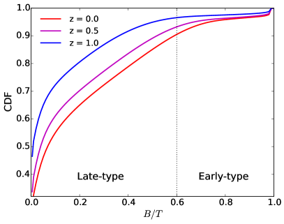
To describe the morphology of a galaxy, we use the ratio between the bulge and the total mass ($B/T$), which can be predicted from the semi-analytical model, as the classification of ‘early-type’ and ‘late-type’ galaxies (Parry et al., 2009). Following Joachimi et al. (2013a), we adopt $B/T=0.6$ to classify the model galaxies into early or late types. Fig. 3 shows the cumulative probability distribution of $B/T$ of our simulated galaxies at three different redshifts. More than $80\%$ of all galaxies are late-types, and the fraction is slightly higher at high redshifts. This fraction of early/late-types is consistent with that found in other studies (e.g., Guo et al., 2013). However, compared to hydro-dynamical simulations, semi-analytical models are less powerful in predicting the shapes of galaxies. To proceed, we have to assign shapes to galaxies and their images with some simplified prescriptions, as described below.

4.2 Galaxy Shape Measurement

A common assumption is that the shape of an elliptical galaxy roughly follows that of its host dark matter halo, while the rotation axis of a spiral galaxy is determined by the spin of its halo (e.g., Kang et al., 2007; Okumura et al., 2009; Agustsson & Brainerd, 2010). Joachimi et al. (2013b, hereafter ’J13’) used this assumption and studied the alignment of galaxies from the Millennium Simulation (Springel et al., 2005). Here we follow J13 to assign shapes to model galaxies.

To assign a shape to a model galaxy using the mass distribution of its dark matter halo, we need to distinguish between central and satellite galaxies. A central galaxy is assumed to be located at the center of a dark matter halo and its shape may be related to that of the host halo. The shape of a dark matter halo is usually defined using the inertia tensor $I_{ij}$ (Bailin & Steinmetz, 2005),

$$I_{ij}=\sum^{N_{\rm p}}_{n=1}{m_{p}x_{i,n},x_{j,n}},$$ (19)

where $N_{\rm p}$ denotes the particle number of the FOF halo, and ${\bf x}_{n}$ is the position of the $n$-th particle with respect to the center of the halo. By diagonalizing the inertia tensor $\bm{I}$, one can get the eigenvalues $\lambda_{1}\leqslant\lambda_{2}\leqslant\lambda_{3}$ and the corresponding eigenvectors that define a triaxial ellipsoid and its orientation. It has been argued that ta minimum number of $N_{\rm p}=300$ is needed to ensure an accurate measurement of the halo shape (Jing, 2002; Bett et al., 2007). Constrained by the resolution of our simulation, we have to reduce the number limit to $100$. As shown in J13, a minimum number of $100$ can lead to $\sim 10\%$ deviation in the axis ratio and $10^{\circ}$ deviation in the orientation angle. Since the magnitude limitation, the corresponding haloes always have more than 100 particles in our mock catalogs for DLS and KiDS-450. Once the three-dimensional shapes and orientations of galaxies are obtained, we project them into the sky to obtain the projected ellipses (Galletta, 1983; Binney, 1985). Details about how to make the projections can be found in appendix B.

In addition to the above model in which perfect alignments are assumed between elliptical galaxies and their host halos, J13 also considered a mis-alignment model in which the major axis of the central elliptical galaxy is mis-aligned with that of the halo, with the mis-alignment angle obeying a gaussian distribution with zero mean and a dispersion of $35^{\circ}$. This is motived by the finding that such a mis-alignment is needed to explain the alignment between luminous red galaxies on large scales (e.g., Kang et al., 2007; Faltenbacher et al., 2009; Okumura et al., 2009; Li et al., 2013). We will come back in Section 5.3.2 to discuss the effect of such mis-alignment on shear correlation functions.

For a central late-type galaxy, defined by $B/T<0.6$, J13 assigned its shape according to the angular momentum vector of the host halo,

$$\bm{L}=\sum^{N_{\rm p}}_{n=1}{m_{p}\bm{x}_{n}\times\bm{v}_{n}},$$ (20)

where $\bm{v}_{n}$ is the velocity of the $n$-th halo particle relative to the halo center. The angular momentum $\bm{L}$ defines a circular disc in the halo, and the complex ellipticity is obtained by projecting the disc along the line of sight. As described in J13, the apparent axis ratio of the projected ellipse is,

$$r=\frac{|L_{{\rm los}}|}{|\bm{L}|}+r_{d}\sqrt{1-\frac{L_{{\rm los}}^{2}}{|\bm{L}|^{2}}},$$ (21)

where $r_{d}$ is the ratio between the disc thickness and diameter, and we set $r_{d}=0.25$ following J13; $L_{{\rm los}}$ is the component of $\bm{L}$ along the line of sight. The ellipticity of the mocked galaxy is then given by

$$\epsilon=(1-r)/(1+r).$$ (22)

For a satellite galaxy, on the other hand, the original dark matter halo associated with it may have suffered strong mass loss after it is accreted into a big halo, depending on the infall time and orbit (Cole et al., 2000). It is thus unclear how the shapes of satellites are connected to those of the dark matter subhaloes associated with them. Some earlier investigations (e.g., Pereira et al., 2008) have shown that the tidal torque of the host halo can induce a correlation between subhalo orientation and its direction to the host center. Therefore, J13 assigned the shape of an early-type satellite galaxy by randomly choosing the three-dimensional axis ratios from a halo sample with more than 300 particles and then made its major axis point to the central galaxy. For a late-type satellite, its spin is assumed to be perpendicular to the line connecting the satellite to the central galaxy, and the ellipticity is obtained by projecting the disk onto the sky, as done for the central spiral galaxies.

The above assumptions for the shapes and orientations of satellite galaxies are clearly too idealistic. In fact, while orbiting in their host halos, satellite galaxies may have their radial alignments scrambled. Observationally, measurements of the shapes of faint satellite galaxies are difficult and sensitive to the methods used to derive galaxy shapes (e.g., Hao et al., 2011). Currently, there is no consensus on the alignments of satellites. Some studies have reported detection of radial alignment of satellites (Pereira & Kuhn, 2005; Agustsson & Brainerd, 2006; Faltenbacher et al., 2007; Chisari et al., 2014; Singh et al., 2015; Huang et al., 2016), while others have not found such an alignment (Siverd et al., 2009; Hao et al., 2011; Schneider et al., 2013; Sifón et al., 2015). Because of this uncertainty, we also consider a simple case in which the orientations of satellites, regardless of their types, are random distributed in their host haloes. We will show in Section 5.3 that satellite alignment has a stronger effect on the shear correlation on smaller scales.

4.3 Intrinsic Shape Correlations of Mock Galaxies

Figure 4: The intrinsic ellipticity correlation, $\eta(r)$, for early-type (upper panel) and late-type (lower panel) central galaxies. Only central galaxies within haloes of mass $m_{{\rm halo}}\geq 3.4\times 10^{10}{\rm M}_{\sun}/h$ (i.e. with 100 particles or more) are used. Early-type galaxies show significant shape alignments and redshift dependence, while for late-types the correlations of their intrinsic ellipticities are very weak. Here errors are estimated using the jackknife method.

Figure 5: Correlation function $\eta(r)$ of early-type galaxies at $z=1.0$. The top panel shows the halo mass dependence of the correlation for galaxies in a given luminosity bin. The bottom panel shows the correlation of galaxies in a given small range of halo mass but with different luminosities. The figure shows that the intrinsic ellipticity correlation is mainly determined by halo mass.

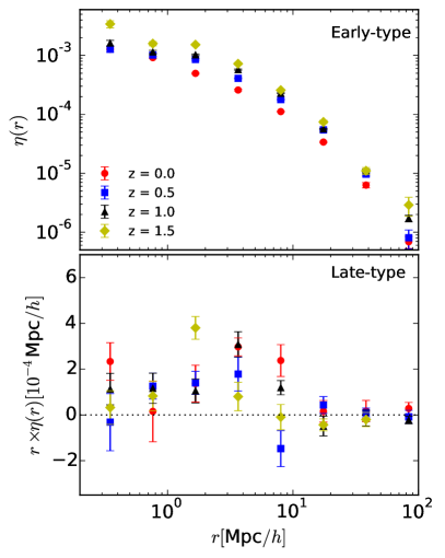
The intrinsic shape correlation function of galaxies, $\eta(r)$, is defined as

$$\eta(r)=\langle\epsilon_{t}(\bm{x})\epsilon_{t}(\bm{x}+\bm{r})+\epsilon_{\times}(\bm{x})\epsilon_{\times}(\bm{x}+\bm{r})\rangle_{\bm{x}},$$ (23)

where $r$ is the three-dimensional comoving separation between two galaxies (e.g., Heymans et al., 2006). The quantities $\epsilon_{t}$ and $\epsilon_{\times}$ are the tangential and cross components of the galaxy ellipticity:

$$\epsilon_{t}+{\rm i}\epsilon_{\times}=-\bm{\epsilon}{\rm e}^{-2{\rm i}\varphi}$$ (24)

where $\varphi$ is the angle between the separation vector of a given galaxy pair and the horizontal axis (Bartelmann & Schneider, 2001).

Following Joachimi et al. (2013b), we first measure the intrinsic shape correlation of galaxies in our simulation by projecting semi-analytic galaxies along the line of sight parallel to the edges of the simulation box. In order to estimate the error bars in our measurements, we divide our simulation box into eight equal-sized cubic sub-boxes of $250\,{\rm Mpc}/h$, and use the Jackknife method to estimate the errors. Fig. 4 shows the redshift dependence of the correlation function $\eta(r)$ for early-type (upper) and late-type (lower) central galaxies in our simulation. It is seen that early-type galaxies have a strong correlation and the correlation is stronger at higher redshifts. In contrast, late-type galaxies do not show any significant correlation of their projected ellipticities, although some weak positive correlation signals can be seen at small scales, $r\lesssim 8{\rm Mpc}/h$. The weak/null correlation for spiral galaxies in our simulation is consistent with the non-detection in both observations (e.g., Mandelbaum et al., 2011) and in simulation results (e.g., Joachimi et al., 2013b).

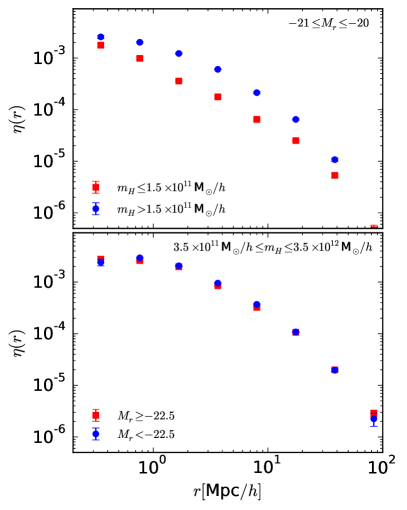
In Fig. 5 we further investigate the dependence of the shear correlation $\eta(r)$ on halo mass and luminosity for early-type galaxies at $z=1.0$. To separate the two dependencies, we select galaxies in a small ranges of luminosity and halo mass, and divide galaxies into two subsamples in halo mass (the top panel) and in galaxy luminosity (the bottom panel ). It can be seen that there is no significant luminosity dependence for fixed halo mass, but a significant dependence on halo mass is seen at a fixed luminosity. This dependence of the intrinsic ellipticity correlation on mass and luminosity in our simulation is similar to the results found in J13.

5 COSMIC SHEAR AND COMPARISON WITH OBSERVATION

5.1 Shear Correlation Function

Weak lensing induces small correlated distortions in observed galaxy shapes. This correlation can be quantified using different statistics. Observationally, the most direct measurement of the lensing signal is the two-point shear correlation function. The shear-shear correlation between galaxies at a given separation $\vartheta$ is estimated as

$$\xi_{tt}(\vartheta)=\frac{\sum_{i,j}w_{i}w_{j}\epsilon_{t,i}\epsilon_{t,j}}{\sum_{i,j}w_{i}w_{j}}$$ (25)

and

$$\xi_{\times\times}(\vartheta)=\frac{\sum_{i,j}w_{i}w_{j}\epsilon_{\times,i}\epsilon_{\times,j}}{\sum_{i,j}w_{i}w_{j}},$$ (26)

where $w_{i}$ is the ellipticity weight of the $i$-th galaxy and $\vartheta$ is the angular separation between the galaxy pair.

The two linear combinations of $\xi_{tt}$ and $\xi_{\times\times}$ that are also frequently used in the lensing analysis are

$$\xi_{\pm}=\xi_{tt}\pm\xi_{\times\times}.$$ (27)

The convergence power spectrum $C^{\kappa\kappa}(\ell)$ can be related to the estimator $\xi_{\pm}$ as

$$\xi_{\pm}(\vartheta)=\frac{1}{2\pi}\int^{\infty}_{0}{\rm d}\ell\ell J_{0,4}(\ell\vartheta)C^{\kappa\kappa}(\ell),$$ (28)

where $J_{0,4}(\ell\vartheta)$ denotes the zeroth and fourth Bessel function for $\xi_{+}$ and $\xi_{-}$, respectively (Schneider et al., 2002).

5.2 Tomographic Cosmic Shear

Tomographic measurement is capable of utilizing the redshift-dependence of cosmic shear signals to reveal both the cosmological structure growth and the redshift-dependent geometry in the universe (King & Schneider, 2003), and has been widely used in weak lensing observations, such as CFHTLens (Heymans et al., 2013), DLS (Jee et al., 2016a), and KiDS-450 (Hildebrandt et al., 2017). In order to perform similar tomographic analysis of cosmic shear in our mock observation and compare the prediction with the KiDS and DLS observations, we employ the tomographic redshift bins as used by Hildebrandt et al. (2017) for KiDS-450 and Jee et al. (2016a) for DLS, to mimic their measurements of cosmic shears.

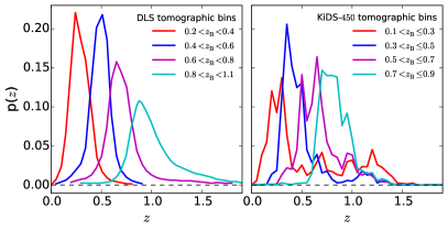
Fig. 6 shows the redshift distributions of the source galaxies in the two surveys, where $z_{\rm B}$ denotes the Bayesian point estimates of the photo-$z$ (Jee et al., 2016a; Hildebrandt et al., 2017). It is seen that the two distributions are quite different. In KiDS-450 the shape of the distribution is not regular, with more overlaps between different redshift bins, while the distribution for DLS is more regular and different bins are more clearly separated. For a consistent comparison between model predictions and observations, we adopt their redshift distributions for the source galaxies respectively, and we truncate source galaxies at $z=2.0$.

To compare with the survey results, we first divide the full-sky into a set of small patches with sizes $\sim 3.6^{\circ}\times 3.6^{\circ}$, and then randomly select $35$ patches in total to cover a field of $\sim 450$ square degrees to match the sky coverage of KiDS-450. By setting a limiting magnitude of $\sim 24.5^{{\rm th}}$ mag in the $r$-band, the effective number density in our light-cone is $n\sim 8\ {\rm arcmin}^{-2}$, similar to that in the KiDS-450 observations. The DLS is much deeper, with a magnitude $\sim 27^{\rm th}$ in $r$-band, producing an effective number density $\sim 11\ {\rm arcmin}^{-2}$ of the source population in 5 tomographic bins. Given that our lensing simulation is performed to redshift $z_{\rm max}\sim 2.0$, we discard the 5th redshift bin, using only tomographic bins 1-4 of DLS, which gives $n\sim 8\ {\rm arcmin}^{-2}$. Thus, a set of mock galaxy catalogue is constructed to mimic the sky coverage and galaxy number density for each of KiDS-450 and DLS. For each mock we produce 100 realizations by randomly sampling the patches at different positions to estimate the uncertainties of tomographic shear correlations due to the cosmic variance and sampling noise.

Figure 6: Redshift distributions of source galaxies in the two weak lensing surveys, DLS (left) and KiDS-450 (right). These redshift distributions are used in our light-cone to select source galaxies and used for the tomographic analyses.

5.3 Results

We measure the auto-correlation and cross-correlation functions $\xi^{(ij)}_{\pm}$ using the public code Athena , which estimates the second-order shear correlation functions from equation (27). The superscript $(ij)$ denotes different redshift bins used for the calculation of the correlation function. In our case there are four redshift bins labeled from $1$ to $4$ with increasing redshift.

5.3.1 Model predictions and comparison with observations

Figure 7: Tomographic measurements of $\xi_{+}$ from our mock KiDS-450 catalogue with galaxy number density $n=8.0\ {\rm arcmin}^{-2}$ and total sky coverage of $\sim 450$ square degrees. Red circles represent the shear correlations from the gravitational field (GG), and black circles are the total shear correlations (GG+II+GI), which can be directly compared with the observational results (blue circles) from the KiDS-450 (Hildebrandt et al., 2017).

Figure 8: Similar to figure 7, but for the tomographic measurements of $\xi_{-}$.

Figure 9: Similar to Fig. 7, but here satellite galaxies are assumed to be radially aligned with the central galaxy while in Fig. 7 satellites are assumed to have random orientations. See the text for details of how we assign galaxy shape and orientation.

Figure 10: Tomographic shear correlations for the DLS mock catalogue with galaxy density $n=8.0\ {\rm arcmin}^{-2}$ and total sky coverage $\sim 20$ square degrees. It is seen that the data points are higher than our model predictions.

Figure 11: Top panels show the contributions of different components to the shear correlations in a few redshift bins, as obtained from our mocked KiDS-450. The lower panels show the ratios of II and GI to the real gravitational shear correlation (GG). In the top panels, solid lines show the results obtained from the best fit to the non-linear alignment model (Eq. 16). Dashed lines show the contributions of GG, II and GI in the model fitting.

Figure 12: The ratios of the II and GI terms with the gravitational shear correlation (GG) in two ideal cases. Top panel: all central galaxies are assumed to be spirals, and their spins are assumed to follow that of the dark matter haloes. Bottom panel: all central galaxies are assumed to be ellipticals, and their shapes are assumed to follow their host haloes but with a mis-alignment that is given by a Gaussian distribution with a dispersion of $35^{\circ}$. It is clearly seen that the GI contribution is positive in the first case, but negative in the second.

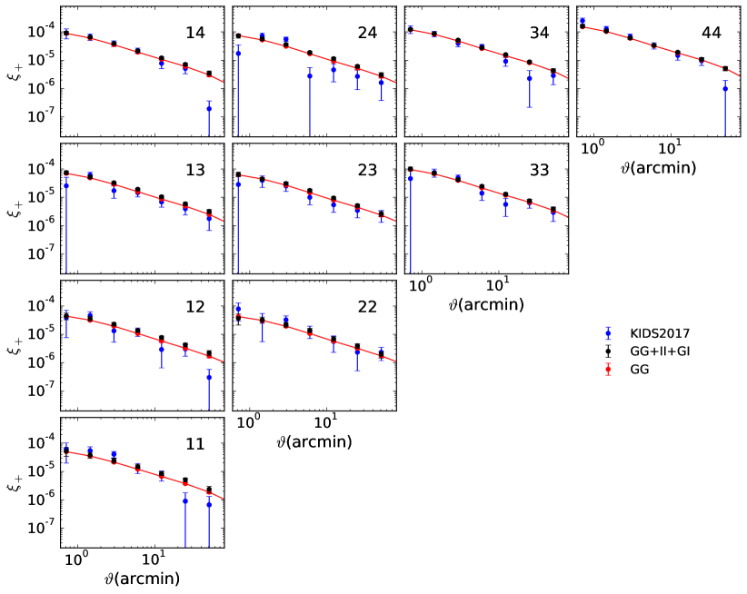
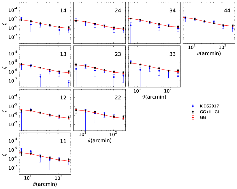
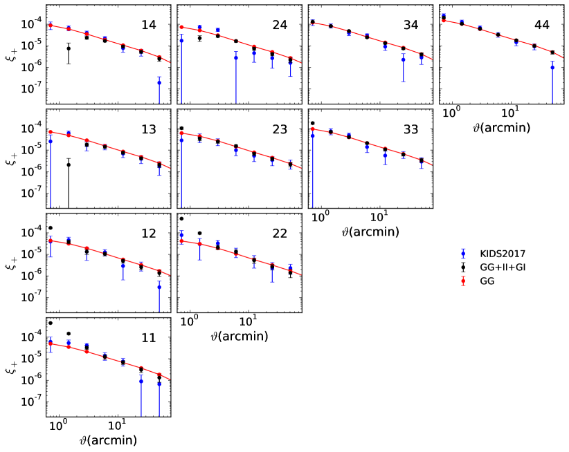
In Figs. 7 and 8 we show the tomographic shear correlations $\xi_{\pm}$ from our model and compare them with the KiDS-450 results. We note that here the orientation of the central galaxy is assumed to follow that of the dark matter halo. Namely for an elliptical central, its major axis follows that of the halo, while for spiral central its orientation is determined by halo spin. For satellite galaxies, regardless of ellipticals or spirals, their orientations are randomly distributed on the sky. The black circles are the model predictions for the ellipticity correlation, which can be directly compared with the data (blue circles). As mentioned in Section 2.3, the predicted ellipticity correlations are combinations of the GG, GI and II correlations. For simplicity, here we only show the GG terms as the red circles connected by the red lines. We will show the contributions of the II and GI terms in Section 5.3.2.

Figs. 7 and 8 show that in general the model predictions (black circles) agree well with the KiDS-450 results. To quantify the difference between the model and the data, we calculate the reduced $\chi^{2}$ defined by

$$\chi^{2}_{\pm}=\frac{1}{n}\sum\frac{(\xi^{\rm M}_{\pm}-\xi^{\rm D}_{\pm})^{2}}{(\sigma^{\rm D}_{\pm})^{2}}.$$ (29)

Here $n$ is the number of data points in the tomographic measurements; $\xi^{\rm M}_{\pm}$ and $\xi^{\rm D}_{\pm}$ represent the predicted and observed tomographic correlations, respectively; $\sigma^{\rm D}_{\pm}$ is the error in the data. The error bars we predicted only contain intrinsic ellipticity dispersion of galaxy, cosmic variance and shot noise, and they represent the dispersion between the results of our 100 realizations, i.e. the uncertainties of one realization. The uncertainties of $\xi_{\pm}^{\rm M}$ which we predicted (the mean of 100 realization) are very low, so we do not take them into account in Eq. 29. We then find the reduced $\chi^{2}_{+(-)}=1.70\ (1.82)$ between our model prediction and the KiDS-450 results. If the correlation between $\xi_{+}$ and $\xi_{-}$ is taken into account, we should estimate the reduced $\chi^{2}$ from the correlation matrix,

$$\chi^{2}=\frac{1}{n}\sum_{i,j}\Delta\xi_{i}C_{ij}^{-1}\Delta\xi_{j},$$ (30)

where $C_{ij}$ is the covariance matrix of the data (Hildebrandt et al., 2017); $\Delta\xi_{i}$ is the difference between the model prediction and the data in the $i$-th separation bin. This gives a reduced $\chi^{2}=1.36$ for the full data vector of KiDS-450, which is slightly higher than the reduced $\chi^{2}=1.33$ in the fiducial analysis of KiDS-450 (Hildebrandt et al., 2017). If we calculate the reduced $\chi^{2}$ for $\xi_{+}$ and $\xi_{-}$ separately, we find $\chi^{2}=1.23$ and $1.61$, respectively.

The good agreement between our model and the KiDS-450 data is encouraging, as this is the first time to reproduce the observational results using lensed images of mock galaxies in N-body simulations combined with a realistic model of galaxy formation. However, inspecting Fig. 7 carefully, one can see that for some bins, such as 12, 24 and 34, the model predictions are slightly higher than the data on large scales. Note that the error bars are also larger in these bins and the data points are not well described by the best fitting model of Hildebrandt et al. (2017). To further quantify the systematic deviation between our model prediction and the data, we define the weighted mean deviation as,

$$\Delta_{\rm m}=\frac{1}{n}\sum\frac{\Delta\xi_{i}}{\sigma_{i}}.$$ (31)

Here only errors from the data are used as the weight $\sigma_{i}$, and the correlation between the measurements is not accounted for. Note that the correlation between the measurements will sightly reduce the deviation, similar to previous analyses for the reduced $\chi^{2}$. The systematic bias between the simulations and the observed data can then be estimated in terms of the standard deviation as

$$S=\frac{\Delta_{\rm m}}{\sigma_{\rm m}},$$ (32)

where $\sigma_{\rm m}=1/\sqrt{n}$ is the scatter of $\Delta_{\rm m}$. In this way, we find that the systematic bias between our model prediction and KiDS-450 result is $S=1.80$ and $1.92$ for $\xi_{+}$ and $\xi_{-}$, respectively. This positive deviation suggests that our predicted correlations are slightly, but systematically higher than the KiDS-450 data with a significance of $\sim 1.8\sigma$. As the error bars are often correlated between different redshift bins, our analyses of these derivations might be too simplistic. However, we do not intend to quantify the difference between the model and the data in detail, but would like to point out that such a difference could be due to the cosmological parameter, $\sigma_{8}\sqrt{\Omega_{\rm m}/0.3}=0.79$, adopted in our simulation, which is slightly larger than that derived one, $0.745\pm 0.039$, from the KiDS-450 data (Hildebrandt et al., 2017).

The results shown in Figs. 7 and 8 assume that satellites have random orientations. In Joachimi et al. (2013b) the orientations of satellite galaxies are assumed to be radially aligned with central galaxies. Thus, for an early-type satellite, its major axis is assumed to point towards to the central galaxy, while for a late-type satellite, its spin is assumed to be perpendicular to the line connecting the satellite to the central galaxy. In Fig. 9 we compare the model results obtained by assuming such radial alignments to the KiDS-450 results. We can see that the shear correlations in diagonal panels at lower redshift are much higher than the data on small scales, except for the highest redshift, 4-4 bin, where the model prediction is close to the data. This indicates that the radial alignment model of satellites produces too strong correlation on small scales. In addition, this model also leads to a strong negative GI term, suppressing the measured total signal on small scales in the cross-correlation of shears, as seen in the off-diagonal bins (13, 14, 24). This strong positive correlation at small scales in the auto-correlation bins, and the strong negative correlation in the cross bins can be explained by the balance between the contributions of the II term and the GI term. With the J13 assumption for satellites, the II term is positive and GI term is negative. In the auto-correlation bins, the II term is stronger than the GI term, so as to make a strong positive correlation of total signal at small scales, as shown in Fig. 9. On the other hand, in the cross-correlation bins, the contribution of the II term is reduced relative to the GI term, so that the correlation at the small scales shows a strong negative correlation in the cross-correlation bins. The reduced $\chi^{2}$ can be calculated from the covariance matrix of the data, and we find $\chi^{2}=3.73$ for the full data vector of KiDS. Calculating the $\chi^{2}$ separately for $\xi_{+}$ and $\xi_{-}$, we get $\chi^{2}=4.63$ and $2.76$, respectively. The results in Fig. 9, therefore, suggest that the radial alignment model for satellite galaxies can be rejected. In what follows, we will only show model predictions in which satellites are assumed to have random orientations.

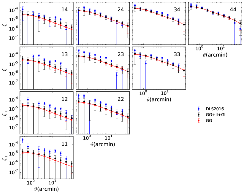
DLS is another weak lensing survey completed recently (Jee et al., 2013, 2016a, 2016b). Compared to KiDS-450, DLS has a smaller sky coverage of 20 square degrees. We produce mock DLS catalogues following its sky coverage, galaxy number density and redshift distribution of source galaxies (see Fig. 6). Our model predictions and comparisons with DLS are shown in Fig. 10. Considering that the data of $\xi_{-}$ is not available for DLS (Jee et al., 2016a), here we only present the results of tomographic correlations $\xi_{+}$. It is seen that the model results (black circles) are lower than the DLS data (blue circles), especially in the lower redshift bins. Note that the error bars in the model is slightly larger. For a DLS-like survey, the reduced $\chi_{+}^{2}=1.56$, and the systematic bias between the simulation and the data is $S=-2.57$ for $\xi_{+}$. The lower reduced $\chi_{+}^{2}$ seems to indicate that the agreement between our model and DLS is slightly better than the agreement with KiDS-450. However, it is clear that the lower reduced $\chi_{+}^{2}$ is also related to the fact the error-bars in DLS data are much larger than those of the KiDS. The large error bars in the DLS data are partly due to its small sky coverage and the smaller sample of galaxies. In the tomographic analysis the KiDS-450 sample is more than 10 times as large as DLS in terms of the total number of galaxies. The strong negative systematic bias $S=-2.57$ indicate that the DLS data are systematically higher than our model predictions. Since the cosmic variance has been taken into account in the error bar of DLS, such a large systematic deviation can hardly be explained by the cosmic variance only.

It is unclear what causes the discrepancy ($\sim 2\sigma$ in $S_{8}$) between the observational results of DLS and KiDS-450. One potential cause might be from the estimations of photo-$z$. For KiDS (Hildebrandt et al., 2017), the DIR method is used to estimate the redshift distribution of galaxies, while for DLS Jee et al. (2016a) the BPZ method is adopted. As briefly discussed in Hildebrandt et al. (2017), the $\chi^{2}$ can increase by $\sim 10$ when switching from the DIR redshift distribution to the BPZ distribution. They also argued that the deeper DLS data is harder to be calibrated. It is beyond our scope to discuss the discrepancy between the KiDS-450 and DLS results in detail. We refer the reader to the paper cited above for more discussions.

5.3.2 The contributions of II and GI terms

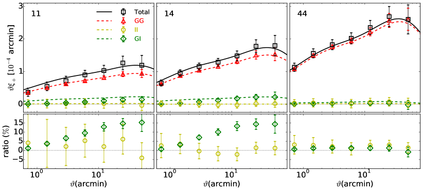
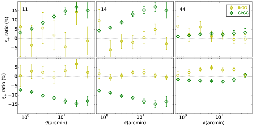
Our previous model results in Fig. 7 show that there is a difference around 10 per cent between the GG term and the total shear correlation. The difference is due to a combination of II and GI terms. In Fig. 11 we show the contributions from the two components separately. As some data points are negative, we plot the $\theta\xi_{+}$ in linear scales, and for clarity, we do not show the observational data. The top panel shows our fiducial results for the KiDS-450 mock in some tomographic redshift bins (the same as in Fig. 7), and the lower panel shows the ratios of GI and II with the GG term. As one can see from the plot, the II term is very weak, consistent with zero. This is expected because most galaxies in our model are late-types and their intrinsic alignment is very weak (Fig. 4). Moreover, the GI term is basically positive and its contribution could be as large as 15% on large scales. Following the procedures usually adopted in observational work to determine the free parameter $A_{\rm IA}$ (e.g., Heymans et al., 2013), we fit the total signals (black circles) from simulation using the non-linear intrinsic alignment model (Eq. 16). Note that in our calculation, the GG signal is given using the non-linear theoretical power spectrum with given cosmological parameters, and the red dashed line in Fig. 11 shows that the theoretical prediction agrees well with the measured GG term from our simulation. The best fit to total signal (GG+II+GI) gives $A_{\rm IA}=-0.972\pm 0.217$. The fit to each component is also shown as the dashed line in the Fig. 11.

Compared with the result by Hildebrandt et al. (2017), they constrained the amplitude of the intrinsic alignment to a positive $A_{\rm IA}=1.10\pm 0.64$ in their fiducial analysis of KiDS-450, which gives a negative GI term in the measurements. While a negative $A_{\rm IA}$ here indicates the contribution from GI term is positive and acts to increase the overall correlation signals. In fact, a positive GI signal is not surprising and has been reported in major weak lensing surveys. For example, Fu et al. (2008) found that $A_{\rm IA}=-2.2^{+4.6}_{-3.8}$ from the third-year CFHTLenS data, and Heymans et al. (2013) reported that $A_{\rm IA}=-1.18^{+0.96}_{-1.17}$ from the final CFHTLenS data. Joudaki et al. (2017) found that $A_{\rm IA}=-3.6\pm 1.6$ from the re-analysis of CFHTLenS data. Hildebrandt et al. (2017) found a positive GI term with $A_{\rm IA}=-1.10_{-0.70}^{+0.96}$ for the KiDS-450 data if they used the BPZ method to estimate galaxy photometric redshift. Recently, Troxel et al. (2017) found, from the DES data, that for spiral galaxies, the GI term is also positive with $A_{\rm IA}=-0.8$ at a 84 per cent confidence level.

Since most galaxies in our model are late-types, we conclude that the positive GI signal is contributed by spirals. As a further test on the contributions from spiral and elliptical galaxies, we show, in Fig. 12, the ratios of the II and GI terms with the GG term for two ideal cases. In the top panel, we assume that all central galaxies in our model are spirals and their spins follow the spins of their host dark matter halos. In the bottom panel, we assume all central galaxies are ellipticals and their shapes follow the shapes of the host halos defined with the inertia tensor, but with a misalignment given by a gaussian distribution with a dispersion of $35^{\circ}$. In the two cases all satellite galaxies are assumed to have random orientations. Fig. 12 shows that the GI term is indeed positive on all scales for spiral galaxies, although their II contribution is close to zero. For elliptical galaxies, their II term is positive and the GI term is negative. Note here the error bars are different for the two different ratios. This can be simply explained from Eq. 15 by considering the noise in the correlation of GI and II terms. As show by the GG correlation, the gravitational shear can be accurately measured in the mock. So if we consider the noise (${\bm{N}}$) in the measurement of intrinsic shapes of galaxies, GI and II terms can be expressed as $\left<{\bm{\epsilon}}_{i}^{\rm(I)}{\bm{g}}_{j}\right>+\left<{\bm{N}}_{i}{\bm{g}}_{j}\right>$ and $\left<{\bm{\epsilon}}_{i}^{\rm(I)}{\bm{\epsilon}}_{j}^{\rm(I)}\right>+2\left<{\bm{\epsilon}}_{i}^{\rm(I)}{\bm{N}}_{j}\right>+\left<{\bm{N}}_{i}{\bm{N}}_{j}\right>$, respectively. The effect of shape noise can contribute the additional correlations as $\left<{\bm{N}}_{i}{\bm{g}}_{j}\right>$ for GI term and $2\left<{\bm{\epsilon}}_{i}^{\rm(I)}{\bm{N}}_{j}\right>+\left<{\bm{N}}_{i}{\bm{N}}_{j}\right>$ for II term. Combining with the definition of correlation $\xi_{+}$, this difference can be used to explain the different error bars for the two different ratios.

A positive GI term from spiral galaxies is not expected from the tidal field model. From linear theory (e.g., Hirata & Seljak, 2004), the GI term is found to be negative, which has been used as a fiducial model in weak lensing data analyses (e.g., Joachimi et al., 2011; Heymans et al., 2013). One important assumption in the linear model is that the shape of foreground galaxies are radially aligned with the nearby over-dense region. This is on average true for elliptical galaxies. But for spiral galaxies, where alignments are mainly determined by angular momenta of the dark matter halos through large-scale tidal field (see Schäfer, 2009, and references therein), this may not be true. Observationally, it is found the spins of spiral galaxies tend to align with the nearby filaments, but the short axes of ellipticals are perpendicular to filaments (Jones et al., 2010; Tempel & Libeskind, 2013). Both hydro-dynamical simulations (e.g., Codis et al., 2015) and N-body simulations (e.g., Kang & Wang, 2015; Wang & Kang, 2017) also confirmed such a dependence on galaxy types. In particular, Chisari et al. (2015) have found from hydro-dynamical simulations that spiral galaxies have a significant tendency to be tangentially aligned with over-density regions. Their figure 10 demonstrates clearly the alignment of spiral galaxies around over-density regions and the origin of a positive GI term.

Finally we note that the II and GI terms are close related to how we model galaxy shapes and orientations. In this paper we simply assume that spiral galaxies follow the spins of dark matter halos. However, as shown in, e.g., Bett et al. (2010), galaxy spins have a broad distribution of mis-alignment with dark matter haloes. This mis-alignment will reduce the positive GI terms. Furthermore, the total GI and II terms in real data depend also on the fraction of spiral and elliptical galaxies, as well as on galaxy luminosities and redshift. More comprehensive analyses on these factors are needed to quantify their impacts on GI and II terms. This paper, which makes use of both $N$-body simulation and galaxies from a semi-analytical model, is a step towards this goal. But here we only focus on a first comparison of the predicted shear correlations with the data. We will present a more comprehensive investigation on the contribution of GI and II terms in a future paper.

6 CONCLUSIONS

It is well known that the intrinsic alignment of galaxy and its associated correlation with the gravitational shear is one of the dominant contaminations to the weak lensing survey. Numerous efforts have been devoted to modeling galaxy-galaxy intrinsic alignment, gravitational-galaxy intrinsic alignment and their impacts on the measure cosmic shear correlation (for a review, see Troxel & Ishak, 2015; Joachimi et al., 2015; Kirk et al., 2015; Kiessling et al., 2015). One useful and direct way to judge these alignment models and their impacts on the measured galaxy shear correlations is to produce mocked galaxy images using ray-tracing simulations which can be directly compared with the observational data.

In this work we make a first attempt to use a large cosmological $N$-body simulation, ELUCID, and a semi-analytical model for galaxy formation, to perform a full-sky ray tracing, so as to produce mocked galaxies images and associated gravitational shear field. We compare our results on the tomographic shear correlation with data from two recent weak-lensing surveys, KiDS-450 and DLS. The main results are summarized in the following.

To produce galaxies images on a curved sky, which is needed for a survey with a large sky coverage, we follow the methods of Becker (2013), and perform a high-spatial and mass resolution ray tracing with an iterative scheme of spherical harmonic analysis. We compare the measured power spectrum of convergence and shear with the analytical Halofit model and the Born approximation. It is found that the measured power spectrums of convergence and shear E-/B-mode have good agreement with the revised non-linear Halofit prediction (Takahashi et al., 2012). The prediction from Born approximation gives higher power at small scales than ray-tracing simulation with $>10\%$ for $\ell\geq 6000$.

We follow Joachimi et al. (2013a, b) to assign shapes to model galaxies. For an early-type central galaxy, its major axis is assumed to align with that of the host dark matter halo, and for late-type central galaxy its spin follows that of the halo with major axis determined by projecting the circular disk on the sky. For early-type satellite galaxies, they are radially aligned with the central galaxy, and for late-type satellites their spin lies in the plane perpendicular to the radial direction to the central galaxy. We also consider an additional model in which satellite galaxies have random orientations. Using this modes for galaxy shapes, we find that early-type central galaxies have strong intrinsic ellipticity correlation but late-type galaxies have very weak alignment, in broad agreement with observations.

To compare with the observational data of KiDS-450 and DLS, we produce mock surveys by mimicking their sky coverage, galaxy number density and redshift distribution of source galaxies. It is found that our model with random orientation of satellites agrees well with KiDS-450. Using the covariance matrix of the data (Hildebrandt et al., 2017), we can follow the Eq. 30 to give the reduced $\chi^{2}=1.36$ for the full data vector of KiD-450. This reduced $\chi^{2}$ is slightly higher than that in the fiducial analysis of KiDS-450, where they obtain a reduced $\chi^{2}=1.33$ (Hildebrandt et al., 2017). In addition, we also calculate the reduced $\chi^{2}$ for $\xi_{+}$ and $\xi_{-}$ separately, and we find the reduced $\chi^{2}$ is 1.23 and 1.61 respectively. To further quantity the difference between our model prediction and the data, we estimate this systematic bias $S$ by Eq. 32. The result shows that the systematic bias between our model prediction and KiDS-450 result is $S=1.80$ and $1.92$ for $\xi_{+}$ and $\xi_{-}$, respectively. In other words, the $\xi_{\pm}$ we predicted are systematically higher than what KiDS measured with a significance of $\sim 1.8\sigma$.

On other hand, considering that the data of $\xi_{-}$ is not available for the DLS data, we only compare our model prediction with the data in $\xi_{+}$. Following Eq. 29, we calculate the reduced $\chi_{+}^{2}$ between the simulation and the data is $1.56$ for the DLS data, which seems to be acceptable in our work. While we also find a strong negative systematic bias $S=-2.57$ between the model prediction and the DLS result, which indicates that the DLS data are systematically higher than our model predictions. Since the cosmic variance has been taken into account in the error bar of DLS, such a large systematic deviation can hardly be explained by the cosmic variance only. Moreover, assuming that there is no scatter in the alignment angle, we rule out the model in which satellite galaxies are radially aligned with central galaxies, as it produces too strong power on small scales.

We also study the contributions of the II and GI terms on the total shear correlations. It is found that the II term is consistent with zero, as in our model most galaxies are spirals and they have very weak intrinsic alignment. Most importantly, we detect a positive GI term which is mainly contributed by spiral galaxies. The GI term can be up to 15 per cent on large scales, and so its effect on the total shear correlation cannot be neglected. A positive GI term is a result of the correlation between the spins of spirals and the large-scale structure, where it is found that spiral galaxies are significantly tangential aligned with the nearby over-dense regions. This alignment is different from that of elliptical galaxies, which are radially aligned with the over-dense regions, and produces a negative GI term.

Finally, we note that in our simulation the shape orientation of model galaxies is determined by the host dark matter halo, which is probably too simplistic. In fact, there should be mis-alignments for both elliptical and spiral galaxies. Quantifying these mis-alignments and their dependence on galaxy properties with observations or hydro-dynamical simulations is crucial. Our results suggest that an accurate model of GI term is very important for weak-lensing survey, and it must include the dependence on galaxy type.

Appendix A Spherical lensing simulation

Here we briefly summarize our multi-sphere ray-tracing algorithm on curved sky. We refer the reader to Das & Bode (2008), Teyssier et al. (2009), Becker (2013) for a detailed description of the full-sky lensing simulation. As described by Becker (2013), lensing properties of our mock galaxies can be extracted from those simulations through an HEALPix grid search method.

A.1 Full-sky Lensing Potential and Ray-tracing

After decomposing the light-cone into a set of shells with the width of $\sim 50h^{-1}{\rm Mpc}$, we can obtain the surface matter overdensity $\sigma^{(n)}$ of the $n$-th shell by

$$\sigma^{(n)}(\bm{\theta}^{(n)})=\int^{\chi_{n+1/2}}_{\chi_{n-1/2}}{\rm d}\chi^{\prime}\delta(r(\chi^{\prime})\bm{\theta}^{(n)},\chi^{\prime}),$$ (A1)

The convergence field is then given by

$$\kappa^{(n)}(\bm{\theta}^{(n)})=W^{(n)}\sigma^{(n)}(\bm{\theta}^{(n)}),$$ (A2)

where the lensing kernel $W^{(n)}$ is defined as

$$W^{(n)}=\frac{3}{2}\left(\frac{H_{0}}{c}\right)^{2}\Omega_{{\rm m}}\frac{r(\chi_{n})}{a(\chi_{n})}$$ (A3)

By solving Poisson equation, one can obtain the lensing potential in harmonic space

$$\phi^{(n)}_{\ell m}=-\frac{2}{\ell(\ell+1)}\kappa^{(n)}_{\ell m}.$$ (A4)

In the context of gravitational lensing, the deflection field $\alpha^{(n)}_{\ell m}$ can be derived from the gravitational lensing potential through equation (18) and light rays can be propagated to the next shells following (Teyssier et al., 2009),

$$\bm{x}^{(n+1)}=\mathcal{R}(\bm{n}^{(n)}\times\bm{\alpha}^{(n)},\lVert\bm{\alpha}^{(n)}\rVert)\bm{x}^{(n)},$$ (A5)

where the rays are initialized at the center of each HEALPix-cell. The rotation matrix $\mathcal{R}$ defines the propagation direction between different shells. The lensing distortion matrix $\mathcal{A}^{(n)}$ can be evaluated by (Becker, 2013),

$$\mathcal{A}^{(n+1)}_{ij} =\left(1-\frac{D^{n}_{0}}{D^{n+1}_{0}}\frac{D^{n+1}_{n-1}}{D^{n}_{n-1}}\right)\mathcal{A}^{(n-1)}_{ij}+\frac{D^{n}_{0}}{D^{n+1}_{0}}\frac{D^{n+1}_{n-1}}{D^{n}_{n-1}}\mathcal{A}^{(n)}_{ij}-\frac{D^{n+1}_{n}}{D^{n+1}_{0}}\mathcal{U}^{(n)}_{ik}\mathcal{A}^{(n)}_{ij},$$ (A6)

where the angular diameter distance $D^{n+1}_{n}\equiv r(\chi_{n+1}-\chi_{n})$; $\mathcal{U}^{(n)}_{ij}$ is the tidal matrix of the $n$-th shell, which can be related to the $2$nd derivatives of the lensing potential, $\mathcal{U}^{(n)}_{ij}=\phi^{(n)}_{,ij}$.

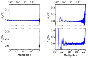
For more accurate computations, we perform the spherical harmonic analysis with an iterative algorithm, as is performed in HEALPix subroutine map2alm_iterative, to control the residual in the solution of the lensing potential. The order of iteration in the analysis is chosen to be 3, as a compromise with the computational time. In Figure 13, we show the statistical measurements with or without this iterative method. Here we define the relative deviation as $\Delta=[C_{0}(\ell)-C_{3}(\ell)]/C_{3}(\ell)$, where the subscript denotes the order of iteration. Clearly, via the iterative algorithm, the numerical errors are controlled effectively, and the power spectra of shear B-mode is significantly suppressed, especially for scales smaller than $\sim 1\ {\rm arcmin}$. It is also more accurate than the multigrid method used in the CALCLENS as discussed in Becker (2013).

Figure 13: The differences of lensing power spectra measured from our ray-tracing simulation with or without the iterative algorithm. Here we defined the relative deviation as $\Delta=[C_{0}(\ell)-C_{3}(\ell)]/C_{3}(\ell)$, where the subscript denotes the order of iteration.

Appendix B Projection of Early-type Galaxy on the Sky

As described in section 4, the intrinsic shape of early-type galaxies can be modeled by the inertial tensor, which defines a triaxial ellipsoid in the intrinsic reference system as,

$$x^{2}+y^{2}/p^{2}+z^{2}/q^{2}=1,$$ (B1)

where the axis ratio satisfies $0<q\leqslant p\leqslant 1$. We follow Galletta (1983) to implement the projection onto the sky. The line of sight is defined by the view angle $(\theta,\varphi)$ in the local coordinate. The axis ratio of the projected ellipse on the sky plane can be written as (Stark, 1977)

$$r(p,q,\theta,\varphi)=\left[\frac{A+C-\sqrt{(A-C)^{2}+B^{2}}}{A+C+\sqrt{(A-C)^{2}+B^{2}}}\right]^{1/2},$$ (B2)

where

$$\begin{cases}A=q^{2}\sin^{2}\theta+(p^{2}\sin^{2}\varphi+\cos^{2}\varphi)\ \cos^{2}\theta\\ B=(1-p^{2})\ \sin 2\varphi\ \cos\theta\\ C=\sin^{2}\varphi+p^{2}\cos^{2}\varphi\end{cases}$$ (B3)

Finally we change the reference system to the observer’s frame to obtain the projected ellipses on the full-sky.

References

- Agustsson & Brainerd (2010) Agustsson, I., & Brainerd, T. G. 2010, ApJ, 709, 1321
- Agustsson & Brainerd (2006) Agustsson, I., & Brainerd, T. G. 2006, ApJ, 644, L25
- Bailin & Steinmetz (2005) Bailin, J., & Steinmetz, M. 2005, ApJ, 627, 647
- Baldry et al. (2008) Baldry, I. K., Glazebrook, K., & Driver, S. P. 2008, MNRAS, 388, 945
- Bartelmann & Schneider (2001) Bartelmann, M., & Schneider, P. 2001, Phys. Rep., 340, 291
- Bartelmann & Maturi (2016) Bartelmann, M., & Maturi, M. 2016, arXiv:1612.06535
- Battye et al. (2015) Battye, R. A., Moss, A., & Pearson, J. A. 2015, J. Cosmology Astropart. Phys, 4, 048
- Becker (2013) Becker, M. R. 2013, MNRAS, 435, 115
- Bett et al. (2007) Bett, P., Eke, V., Frenk, C. S., et al. 2007, MNRAS, 376, 215
- Bett et al. (2010) Bett, P., Eke, V., Frenk, C. S., Jenkins, A., & Okamoto, T. 2010, MNRAS, 404, 1137
- Binney (1985) Binney, J. 1985, MNRAS, 212, 767
- Blazek et al. (2012) Blazek, J., Mandelbaum, R., Seljak, U., & Nakajima, R. 2012, J. Cosmology Astropart. Phys, 5, 041
- Bridle & King (2007) Bridle, S., & King, L. 2007, New Journal of Physics, 9, 444
- Bunn (2003) Bunn, E. F. 2003, New A Rev., 47, 987
- Bunn et al. (2003) Bunn, E. F., Zaldarriaga, M., Tegmark, M., & de Oliveira-Costa, A. 2003, Phys. Rev. D, 67, 023501
- Calabretta & Roukema (2007) Calabretta, M. R., & Roukema, B. F. 2007, MNRAS, 381, 865
- Catelan et al. (2001) Catelan, P., Kamionkowski, M., & Blandford R. D. 2001, MNRAS, 320, 7
- Catelan & Porciani (2001) Catelan, P., & Porciani, C. 2001, MNRAS, 323, 713
- Chisari et al. (2015) Chisari, N., Codis, S., Laigle, C., et al. 2015, MNRAS, 454, 2736
- Chisari et al. (2016) Chisari, N., Laigle, C., Codis, S., et al. 2016, MNRAS, 461, 2702
- Chisari et al. (2017) Chisari, N. E., Koukoufilippas, N., Jindal, A., et al. 2017, MNRAS, 472, 1163
- Chisari et al. (2014) Chisari, N. E., Mandelbaum, R., Strauss, M. A., Huff, E. M., & Bahcall, N. A. 2014, MNRAS, 445, 726
- Codis et al. (2015) Codis, S., Gavazzi, R., Dubois, Y., et al. 2015, MNRAS, 448, 3391
- Cole et al. (2000) Cole, S., Lacey, C. G., Baugh, C. M., & Frenk, C. S. 2000, MNRAS, 319, 168
- Cooray & Hu (2002) Cooray, A., & Hu, W. 2002, ApJ, 574, 19
- Crittenden et al. (2001) Crittenden, R. G., Natarajan, P., Pen, U.-L., & Theuns, T. 2001, ApJ, 559, 552
- Dark Energy Survey Collaboration et al. (2016) Dark Energy Survey Collaboration, Abbott, T., Abdalla, F. B., et al. 2016, MNRAS, 460, 1270
- Das & Bode (2008) Das, S., & Bode, P. 2008, ApJ, 682, 1-13
- de Jong et al. (2015) de Jong, J. T. A., Verdoes Kleijn, G. A., Boxhoorn, D. R., et al. 2015, A&A, 582, A62
- Dong et al. (2014) Dong, X. C., Lin, W. P., Kang, X., et al. 2014, ApJ, 791, L33
- Faltenbacher et al. (2007) Faltenbacher, A., Li, C., Mao, S., et al. 2007, ApJ, 662, L71
- Faltenbacher et al. (2009) Faltenbacher, A., Li, C., White, S. D. M., et al. 2009, Research in Astronomy and Astrophysics, 9, 41
- Foreman et al. (2016) Foreman, S., Becker, M. R., & Wechsler, R. H. 2016, MNRAS, 463, 3326
- Fosalba et al. (2015) Fosalba, P., Gaztañaga, E., Castander, F. J., & Crocce, M. 2015, MNRAS, 447, 1319
- Fosalba et al. (2008) Fosalba, P., Gaztañaga, E., Castander, F. J., & Manera, M. 2008, MNRAS, 391, 435
- Fu et al. (2008) Fu, L., Semboloni, E., Hoekstra, H., et al. 2008, A&A, 479, 9
- Górski et al. (2005) Górski, K. M., Hivon, E., Banday, A. J., et al. 2005, ApJ, 622, 759
- Galletta (1983) Galletta, G. 1983, Ap&SS, 92, 335
- Guo et al. (2013) Guo, Q., White, S., Angulo, R. E., et al. 2013, MNRAS, 428, 1351
- Hao et al. (2011) Hao, J., Kubo, J. M., Feldmann, R., et al. 2011, ApJ, 740, 39
- Heavens et al. (2000) Heavens, A., Refregier, A., & Heymans, C. 2000, MNRAS, 319, 649
- Heymans et al. (2013) Heymans, C., Grocutt, E., Heavens, A., et al. 2013, MNRAS, 432, 2433
- Heymans et al. (2012) Heymans, C., Van Waerbeke, L., Miller, L., et al. 2012, MNRAS, 427, 146
- Heymans et al. (2006) Heymans, C., White, M., Heavens, A., Vale, C., & van Waerbeke, L. 2006, MNRAS, 371, 750
- Higuchi & Shirasaki (2016) Higuchi, Y., & Shirasaki, M. 2016, MNRAS, 459, 2762
- Hilbert et al. (2009) Hilbert, S., Hartlap, J., White, S. D. M., & Schneider, P. 2009, A&A, 499, 31
- Hilbert et al. (2017) Hilbert, S., Xu, D., Schneider, P., et al. 2017, MNRAS, 468, 790
- Hildebrandt et al. (2017) Hildebrandt, H., Viola, M., Heymans, C., et al. 2017, MNRAS, 465, 1454
- Hinshaw et al. (2013) Hinshaw, G., Larson, D., Komatsu, E., et al. 2013, ApJS, 208, 19
- Hirata & Seljak (2004) Hirata, C. M., & Seljak, U. 2004, Phys. Rev. D, 70, 063526
- Hu (2000) Hu, W. 2000, Phys. Rev. D, 62, 043007
- Huang et al. (2016) Huang, H.-J., Mandelbaum, R., Freeman, P. E., et al. 2016, MNRAS, 463, 222
- Jain et al. (2000) Jain, B., Seljak, U., & White, S. 2000, ApJ, 530, 547
- Jee et al. (2016a) Jee, M. J., Tyson, J. A., Hilbert, S., et al. 2016a, ApJ, 824, 77
- Jee et al. (2013) Jee, M. J., Tyson, J. A., Schneider, M. D., et al. 2013, ApJ, 765, 74
- Jee et al. (2016b) Jee, M. J., Tyson, J. A., Hilbert, S., et al. 2016b, American Astronomical Society Meeting Abstracts, 227, 307.07
- Jing (2002) Jing, Y. P. 2002, MNRAS, 335, L89
- Joachimi et al. (2011) Joachimi, B., Mandelbaum, R., Abdalla, F. B., & Bridle, S. L. 2011, A&A, 527, A26
- Joachimi et al. (2013a) Joachimi, B., Semboloni, E., Bett, P. E., et al. 2013a, MNRAS, 431, 477
- Joachimi et al. (2013b) Joachimi, B., Semboloni, E., Hilbert, S., et al. 2013b, MNRAS, 436, 819
- Joachimi et al. (2015) Joachimi, B., Cacciato, M., Kitching, T. D., et al. 2015, Space Sci. Rev., 193, 1
- Jones et al. (2010) Jones, B. J. T., van de Weygaert, R., & Aragón-Calvo, M. A. 2010, MNRAS, 408, 897
- Joudaki et al. (2017) Joudaki, S., Blake, C., Heymans, C., et al. 2017, MNRAS, 465, 2033
- Kang et al. (2007) Kang, X., van den Bosch, F. C., Yang, X., et al. 2007, MNRAS, 378, 1531
- Kang & Wang (2015) Kang, X., & Wang, P. 2015, ApJ, 813, 6
- Keres et al. (2003) Keres, D., Yun, M. S., & Young, J. S. 2003, ApJ, 582, 659
- Kiessling et al. (2015) Kiessling, A., Cacciato, M., Joachimi, B., et al. 2015, Space Sci. Rev., 193, 67
- Kilbinger (2015) Kilbinger, M. 2015, Reports on Progress in Physics, 78, 086901
- Kilbinger (2003) Kilbinger, M. 2003, arXiv:astro-ph/0309482
- Kilbinger et al. (2017) Kilbinger, M., Heymans, C., Asgari, M., et al. 2017, arXiv:1702.05301
- King & Schneider (2003) King, L. J., & Schneider, P. 2003, A&A, 398, 23
- Kirk et al. (2010) Kirk, D., Bridle, S., & Schneider, M. 2010, MNRAS, 408, 1502
- Kirk et al. (2015) Kirk, D., Brown, M. L., Hoekstra, H., et al. 2015, Space Sci. Rev., 193, 139
- Kitching et al. (2016) Kitching, T. D., Alsing, J., Heavens, A. F., et al. 2016, arXiv:1611.04954
- Komatsu et al. (2011) Komatsu, E., Smith, K. M., Dunkley, J., et al. 2011, ApJS, 192, 18
- Krause et al. (2016) Krause, E., Eifler, T., & Blazek, J. 2016, MNRAS, 456, 207
- Laureijs et al. (2011) Laureijs, R., Amiaux, J., Arduini, S., et al. 2011, arXiv:1110.3193
- Lemos et al. (2017) Lemos, P., Challinor, A., & Efstathiou, G. 2017, J. Cosmology Astropart. Phys, 5, 014
- Levy & Brustein (2009) Levy, D., & Brustein, R. 2009, J. Cosmology Astropart. Phys, 6, 026
- Li & White (2009) Li, C., & White, S. D. M. 2009, MNRAS, 398, 2177
- Li et al. (2005) Li, G.-L., Mao, S., Jing, Y. P., et al. 2005, ApJ, 635, 795
- Li et al. (2012) Li, M., Pan, J., Gao, L., et al. 2012, ApJ, 761, 151
- Li et al. (2016) Li, S.-J., Zhang, Y.-C., Yang, X.-H., et al. 2016, Research in Astronomy and Astrophysics, 16, 130
- Li et al. (2013) Li, Z., Wang, Y., Yang, X., et al. 2013, ApJ, 768, 20
- Ling et al. (2015) Ling, C., Wang, Q., Li, R., et al. 2015, Phys. Rev. D, 92, 064024
- LSST Science Collaboration et al. (2009) LSST Science Collaboration, Abell, P. A., Allison, J., et al. 2009, arXiv:0912.0201
- Luo et al. (2016) Luo, Y., Kang, X., Kauffmann, G., & Fu, J. 2016, MNRAS, 458, 366
- Mandelbaum et al. (2011) Mandelbaum, R., Blake, C., Bridle, S., et al. 2011, MNRAS, 410, 844
- Mandelbaum et al. (2006) Mandelbaum, R., Hirata, C. M., Ishak, M., Seljak, U., & Brinkmann, J. 2006, MNRAS, 367, 611
- Mellier (1999) Mellier, Y. 1999, ARA&A, 37, 127
- Meylan et al. (2006) Meylan, G., Jetzer, P., North, P., et al. 2006, Saas-Fee Advanced Course 33: Gravitational Lensing: Strong, Weak and Micro,
- Miyazaki et al. (2012) Miyazaki, S., Komiyama, Y., Nakaya, H., et al. 2012, Proc. SPIE, 8446, 84460Z
- Okumura et al. (2009) Okumura, T., Jing, Y. P., & Li, C. 2009, ApJ, 694, 214
- Parry et al. (2009) Parry, O. H., Eke, V. R., & Frenk, C. S. 2009, MNRAS, 396, 1972
- Peacock & Smith (2014) Peacock, J. A., & Smith, R. E. 2014, Astrophysics Source Code Library, ascl:1402.032
- Pereira & Kuhn (2005) Pereira, M. J., & Kuhn, J. R. 2005, ApJ, 627, L21
- Pereira et al. (2008) Pereira, M. J., Bryan, G. L., & Gill, S. P. D. 2008, ApJ, 672, 825-833
- Schäfer (2009) Schäfer, B. M. 2009, International Journal of Modern Physics D, 18, 173
- Schneider & Bridle (2010) Schneider, M. D., & Bridle, S. 2010, MNRAS, 402, 2127
- Schneider et al. (2013) Schneider, M. D., Cole, S., Frenk, C. S., et al. 2013, MNRAS, 433, 2727
- Schneider et al. (2002) Schneider, P., van Waerbeke, L., Kilbinger, M., & Mellier, Y. 2002, A&A, 396, 1
- Schneider et al. (2002) Schneider, P., van Waerbeke, L., & Mellier, Y. 2002, A&A, 389, 729
- Schneider et al. (1992) Schneider, P., Ehlers, J., & Falco, E. E. 1992, Gravitational Lenses, XIV, 560 pp. 112 figs.. Springer-Verlag Berlin Heidelberg New York. Also Astronomy and Astrophysics Library, 112
- Shirasaki et al. (2015) Shirasaki, M., Hamana, T., & Yoshida, N. 2015, MNRAS, 453, 3043
- Sifón et al. (2015) Sifón, C., Hoekstra, H., Cacciato, M., et al. 2015, A&A, 575, A48
- Singh et al. (2015) Singh, S., Mandelbaum, R., & More, S. 2015, MNRAS, 450, 2195
- Siverd et al. (2009) Siverd, R. J., Ryden, B. S., & Gaudi, B. S. 2009, arXiv:0903.2264
- Smith et al. (2003) Smith, R. E., Peacock, J. A., Jenkins, A., et al. 2003, MNRAS, 341, 1311
- Springel (2010) Springel, V. 2010, ARA&A, 48, 391
- Springel (2005) Springel, V. 2005, MNRAS, 364, 1105
- Springel et al. (2005) Springel, V., White, S. D. M., Jenkins, A., et al. 2005, Nature, 435, 629
- Springel et al. (2001) Springel, V., White, S. D. M., Tormen, G., & Kauffmann, G. 2001, MNRAS, 328, 726
- Stark (1977) Stark, A. A. 1977, ApJ, 213, 368
- Stebbins (1996) Stebbins, A. 1996, arXiv:astro-ph/9609149
- Takahashi et al. (2012) Takahashi, R., Sato, M., Nishimichi, T., Taruya, A., & Oguri, M. 2012, ApJ, 761, 152
- Tempel & Libeskind (2013) Tempel, E., & Libeskind, N. I. 2013, ApJ, 775, L42
- Tenneti et al. (2016) Tenneti, A., Mandelbaum, R., & Di Matteo, T. 2016, MNRAS, 462, 2668
- Tenneti et al. (2014) Tenneti, A., Mandelbaum, R., Di Matteo, T., Feng, Y., & Khandai, N. 2014, MNRAS, 441, 470
- Teyssier et al. (2009) Teyssier, R., Pires, S., Prunet, S., et al. 2009, A&A, 497, 335
- Troxel & Ishak (2015) Troxel, M. A., & Ishak, M. 2015, Phys. Rep., 558, 1
- Troxel et al. (2017) Troxel, M. A., MacCrann, N., Zuntz, J., et al. 2017, arXiv:1708.01538
- Tweed et al. (2017) Tweed, D., Yang, X., Wang, H., et al. 2017, arXiv:1704.03675
- Van Waerbeke et al. (2001) Van Waerbeke, L., Mellier, Y., Radovich, M., et al. 2001, A&A, 374, 757
- Velliscig et al. (2015) Velliscig, M., Cacciato, M., Schaye, J., et al. 2015, MNRAS, 454, 3328
- Wang et al. (2014) Wang, H., Mo, H. J., Yang, X., Jing, Y. P., & Lin, W. P. 2014, ApJ, 794, 94
- Wang et al. (2016) Wang, H., Mo, H. J., Yang, X., et al. 2016, ApJ, 831, 164
- Wang & Kang (2017) Wang, P., & Kang, X. 2017, MNRAS, 468, L123
- White & Vale (2004) White, M., & Vale, C. 2004, Astroparticle Physics, 22, 19
- Yang et al. (2006) Yang, X., van den Bosch, F. C., Mo, H. J., et al. 2006, MNRAS, 369, 1293
- York et al. (2000) York, D. G., Adelman, J., Anderson, J. E., Jr., et al. 2000, AJ, 120, 1579
- Zhao & Baskaran (2010) Zhao, W., & Baskaran, D. 2010, Phys. Rev. D, 82, 023001
- Zwaan et al. (2005) Zwaan, M. A., Meyer, M. J., Staveley-Smith, L., & Webster, R. L. 2005, MNRAS, 359, L30