Axionic Landscape for Higgs Near-Criticality

Abstract

The measured value of the Higgs quartic coupling $\lambda$ is peculiarly close to the critical value above which the Higgs potential becomes unstable, when extrapolated to high scales by renormalization group running. It is tempting to speculate that there is an anthropic reason behind this near-criticality. We show how an axionic field can provide a landscape of vacuum states in which $\lambda$ scans. These states are populated during inflation to create a multiverse with different quartic couplings, with a probability distribution $P$ that can be computed. If $P$ is peaked in the anthropically forbidden region of Higgs instability, then the most probable universe compatible with observers would be close to the boundary, as observed. We discuss three scenarios depending on the Higgs vacuum selection mechanism: decay by quantum tunneling; by thermal fluctuations or by inflationary fluctuations.

I Introduction

The standard model (SM) of particle physics, while enjoying tremendous success as an accurate description of nature, has many parameters whose values look mysterious from a theoretical perspective. Why are the Higgs mass and the energy scale of the cosmological constant so small compared to the Planck scale? Why is $\theta_{QCD}$ so small? What is the origin of the hierarchy of fermion masses? Such questions have inspired many efforts to go beyond the standard model. Following the discovery of the Higgs boson, there is a new item, dubbed “Higgs near-criticality,” on the list: why is the Higgs self-coupling $\lambda$ (in conjunction with the top quark Yukawa coupling $y_{t}$) so close to the critical value beyond which the Higgs potential becomes unstable at high scales? The situation is illustrated in fig. 1 STAB , which shows the regions of stability, metastability and instability of our vacuum, in the $\lambda$-$y_{t}$ plane, with the small ellipse of the measured values falling in the narrow region of metastability. In the metastability (instability) region the vacuum lifetime is longer (shorter) than the age of the Universe.

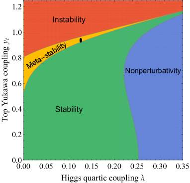
Figure 1: Regions of the $\lambda$-$y_{t}$ plane leading to stability, metastability or instability of the Higgs potential at high scales (at NNLO accuracy STAB ). In the region labeled “Nonperturbativity” $\lambda$ becomes strong below the Planck scale. The couplings are defined at the electroweak scale.

The answer could of course be that it is a coincidence: for fixed $y_{t}$, the quartic coupling is $0.01$ below the stability boundary ($0.03$ above the instability line), which is a tuning of only 8% (23%) relative to its actual value. On the other hand if $\lambda$ could a priori have taken any value between zero and $4\pi$, this becomes a tuning of $0.08\%$ ($0.2\%$), more in accord with the visual impression from fig. 1. This is predicated on the assumption that there is no new physics coupled to the Higgs at high scales (up to the Planck scale) that might shift the stability boundaries relative to where they are shown. Nevertheless since there is an anthropic reason for $\lambda$ to avoid the instability region, it is tempting to construct a scenario where this explains the coincidence.

While anthropic reasoning is eschewed by many physicists, if there is a landscape of vacuum states in which anthropically sensitive parameters are sampled, it seems difficult to dismiss. For example the very large number of flux compactifications in string theory Douglas:2003um ; Ashok:2003gk make it plausible that our universe is part of a much larger multiverse LindeEternal . A solution of the cosmological constant ($\Lambda$) problem was proposed in which $\Lambda$ is finely scanned by these flux vacua BP , yielding values consistent with anthropic bounds Weinberg:1987dv . Coleman’s wormhole mechanism Coleman:1988tj is another example of a multiverse in which the most likely value of $\Lambda$ is small (in fact vanishing).

In this context, Rubakov and Shaposhnikov argued Rubakov:1989pn that the observed values of physical constants might generically be close to the boundaries of the anthropically allowed regions. If the probability distribution is such that the most likely value of a parameter is anthropically forbidden, then the most likely observed value would be close to the boundary, since there are no observers on the forbidden side. The near-criticality of the Higgs potential looks like a possible example of this phenomenon.

The anthropic necessity of Higgs stability is an old observation that was used to put a lower bound on the Higgs mass (or an upper bound on the heaviest quark mass) as early as 1979 Stab0 . Improved predictions using higher orders in the loop expansion were subsequently made STAB ; StabMore . An indication of how delicate the tuning is for near-criticality is provided by the comparison of such predictions at different levels of precision ELattice : at LO our vacuum would be deep in the instability region, at NLO in the middle of the metastable one and at NNLO very close to the stability boundary.

Of particular relevance for our work, the implications of Higgs stability within a landscape of vacua with $\lambda$ scanning were studied in ref.  Hall , assuming conditions just like those suggested by ref. Rubakov:1989pn for the underlying probability distribution $P(\lambda)$, namely that it is maximized in the unstable region of small $\lambda$. In that work, a model-independent analysis was done, where no particular model of the landscape was proposed; rather a reasonable functional form for $P(\lambda)$ was assumed, which led to predictions for the Higgs mass prior to its measurement.

We think it is worthwhile to revisit the question of Higgs near-criticality within a specific model of the landscape, since such a study may reveal nontrivial challenges to the overall consistency of such a picture, that may be shared by other possible examples. At the same time we introduce a new kind of landscape that is particularly simple and amenable to calculations, namely the vacuum states provided by the minima of the potential of an axion field (whose detailed properties are very different from those of the QCD axion).

We are inspired by a string-theory-motivated construction, axion monodromy, previously used for inflation AxMono and by the relaxion mechanism relaxion , used for solving the weak scale hierarchy problem. In contrast to these applications however, we wish to avoid classical evolution of the axion $a$ during cosmological evolution. Instead, the universe is assumed to split into causally disconnected domains where $a$ sits in different local minima of its potential. These vacuum states were populated by quantum fluctuations of $a$ during a period of inflation, are essentially stable against tunneling once formed, and so realize a tractable example of a multiverse. The probability distribution is calculable in terms of the axion potential, given certain assumptions about the cosmological evolution that we will specify.

II Landscape for $\lambda$

The field $a$ has a potential of the form

$$V(a) = \overline{V}(a)-\Lambda_{b}^{4}\cos(a/f)\ ,$$ (1)

where $\overline{V}$ denotes the part of the potential that can be approximated as non-oscillatory on a field range large compared to $2\pi f$. As the field $a$ has an axionic origin ($a$ is a pseudo-Goldstone boson, like a phase field), it originally enjoys a shift symmetry $a\rightarrow a+c$ that is broken by the potential (1). The term $\Lambda_{b}^{4}\cos(a/f)$ breaks the shift symmetry down to a discrete subgroup $a\rightarrow a+2\pi f$, while $\overline{V}(a)$ breaks the shift symmetry completely (at least in the range we consider; see below). It is then natural to expect these breaking terms to be much smaller than the typical mass scale or cutoff of the theory that we will call $\Lambda$. In a string theoretic UV completion, $\Lambda$ could be the string scale.

We assume then $\Lambda_{b}\lesssim\Lambda$ and take $\overline{V}(a)=\Lambda^{4}\ V(\eta a/\Lambda)$, with $\eta\ll 1$. For our purposes it will suffice to keep the linear term of this function:

$$\overline{V}(a)=\eta\Lambda^{3}a+\dots$$ (2)

This linear term should accurately describe the potential $\overline{V}(a)$ in a typical field region. Without loss of generality (by doing a shift in the field), we can take this typical region to be in the vicinity of $a=0$ and we can also take $\eta>0$ so that $\overline{V}(a)$ is a growing function of $a$.

A concrete example for $\overline{V}$ that arises in certain string theory compactifications AxMono is

$$\overline{V}(a)=M^{4}\sqrt{1+a^{2}/F^{2}}\simeq M^{4}a/F,$$ (3)

where the linear approximation is valid in the region where $a\gg F$. Here, $M$ and $F$ are generically at the string scale, but if the axion arises from a warped throat, then $M$ can be parametrically suppressed by a warp factor, which may be exponentially small.

Another example is the clockwork axion clockwork , with $\overline{V}(a)=\epsilon\Lambda^{4}\cos(a/F)$, and $F=Nf\gg f$, which hierarchy can be arranged in a natural way. In this setting, the field range is compact, $2\pi F$, but we are interested in a patch $\Delta a$ with $2\pi f\ll\Delta a\ll 2\pi F$, and there we can expand $\overline{V}(a)$ as in (2) around some typical value $a_{0}$, obtaining $\eta=-(\epsilon\Lambda/F)\sin(a_{0}/F)$.

Let the minima of the potential (1) be labeled by an integer $n$, such that $a_{n}\simeq 2\pi nf$. A basic condition for having a landscape is that $\overline{V}$ must be sufficiently flat so that it does not destroy the local minima of the oscillatory part. This requires

$$\overline{V}{}^{\prime}(a)=\eta\,\Lambda^{3}\lesssim{\Lambda_{b}^{4}\over f}\ ,$$ (4)

which, if satisfied, would naively imply infinitely many local minima. In realistic string constructions however, there is back-reaction from large windings, so that the actual number of minima is limited to $N\lesssim 10-100$, beyond which the above description breaks down, and possibly an extra dimension decompactifies Liam . In clock-work constructions the number of vacua is also finite as the field range is compact.

We assume that in addition to $\overline{V}$, there is a coupling of $a$ to the Higgs potential:

$$V_{h}=\Big{(}-\mu_{h}^{2}+c_{h}\eta\,a\Lambda\Big{)}|H|^{2}+\left(\lambda+c_{\lambda}\,\frac{\eta\,a}{\Lambda}\right)|H|^{4}\ .$$ (5)

Such couplings also break the shift symmetry and so we assign a factor $\eta$ to them. The $a$-terms in (5) could be regarded as arising from a generalization of eq. (3) by taking $M^{4}\to M^{4}+{\cal O}(\Lambda^{2}|H|^{2},|H|^{4})$ or from expanded $\cos(a/F)$ potentials in the clockwork realization. In the landscape of vacua of the $a$ field, where $\langle a\rangle=a_{n}\simeq 2\pi nf$, this shifts the bare values (i.e., the values at the UV scale $\Lambda$) of the Higgs parameters to

$$\mu_{n}^{2} = \mu_{h}^{2}-n\,c_{h}\eta\,(2\pi f)\Lambda\,,$$

$$\lambda_{n} = \lambda+n\,c_{\lambda}\eta\frac{2\pi f}{\Lambda}\equiv\lambda+n\,\delta\lambda\,.$$ (6)

Here we assume that some other mechanism solves the weak scale hierarchy problem (e.g. a relaxion mechanism relaxion ) so that $\mu_{n}$ is of electroweak size and focus on the shift in the Higgs coupling. For reasons detailed below we also choose $c_{\lambda}>0$. Likewise we must assume there is another mechanism for solving the cosmological constant problem, since the vacuum energy varies between $a$-vacua due to the nonperiodic part of the potential $\overline{V}$.

We consider three possible scenarios, each associated to one of the three critical boundaries shown in fig. 2; these are the boundaries of instability and metastability at zero temperature, and the boundary of high-temperature instability that depends upon the assumed reheating temperature (dashed lines). Our mechanism explains why we would observe $(\lambda,y_{t})$ to be near (and to the right of) one of these boundaries. The characteristics of the three categories are summarized in table 1. Fig. 2 shows trajectories of successive vacua that exemplify each case. Which one of the three is actually realized depends upon cosmological parameters, as we will discuss in more detail in the next section.

	(1)	(2)	(3)
Boundary	$T=0$ Instablity	$T_{R}$ Instability	Stability
Vacuum	Quantum	Thermal	Inflationary
Selection	$T=0$ decay	decay	decay
$\delta\lambda$	$\sim 0.05$	$\sim 0.02$	$\ll 0.01$
$M_{t}$/GeV	$173.34\pm 2.28$	$173.34^{+1.34}_{-2.28}$	$\simeq 171$

Table 1: Characteristics of the three cases we consider in the text, regarding the critical boundary, vacuum selection mechanism, step in $\lambda$ needed and range of top mass (inside the experimental $3\sigma$ band) required.

In case (1) we end close to the instability boundary and the probability to live in vacua beyond that boundary is depleted by $T=0$ decay, in which the Higgs vacuum has a lifetime that is shorter than the age of the Universe. To explain why a point lying in the experimentally allowed ellipse at $y_{t}\simeq 0.95$ corresponds to the most probable anthropically allowed vacuum, we need $\delta\lambda\sim 0.05$, the approximate width of the metastable region. Scenario (1) could take place for any value of the top mass, within the experimentally preferred region, which we take to be the 3$\sigma$ range $M_{t}=173.34\pm 3\times 0.67$ GeV top .

In case (2) we end in a vacuum near the instability boundary for decay by thermal fluctuations with a high reheating temperature, that reduce the region of metastability. As concrete examples we illustrate the cases of $T_{R}=10^{14}$ and $T_{R}=10^{16}$ GeV. The boundary of the reduced region is shown as the dashed lines in Fig. 2 (see refs. Tdec ; Higgstory ), and a possible trajectory illustrating this case is shown along $y_{t}\simeq 0.934$. A smaller step size $\delta\lambda\sim 0.02$ is suggested for naturally explaining the distance of the SM point from the dashed boundary. This mechanism, for such large $T_{\rm R}$ favors the lower range of the top mass, with $M_{t}\simeq 173.34^{+1.34}_{-2.28}$ GeV.

In case (3) we end very close to the stability boundary beyond which the Higgs vacuum is unstable against decay during inflation, for sufficiently large values of ${\cal H}_{I}\sqrt{N_{e}}$. This case is illustrated by the trajectory passing through the bottom of the experimental ellipse. Here the most probable state would be the one closest to the boundary in the absolute stability region, and it would require a very small step size $\delta\lambda$ to be naturally close to the experimental ellipse. Although this possibility is currently disfavored, it is not excluded and provides another possible regime for explaining near-critical stability, if the top mass is very close to its lowest $3\sigma$ value, $M_{t}\simeq 171$ GeV.

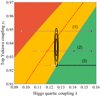
Figure 2: Zoom-in of Fig. 1 showing also the instability lines for thermal vacuum decay with $T_{R}=10^{14-16}$ GeV (red dashed lines). Trajectories of $a$-vacua are shown (surviving ones in black, doomed ones in white) for the three cases discussed in the text. We use $M_{h}=125.09\pm 0.24$ GeV mh and $M_{t}=173.34\pm 0.67$ GeV top at 1-$\sigma$ for the experimental ellipses.

Once $\delta\lambda$ is fixed, (6) can be used to to eliminate the unknown parameter $\eta$ in terms of $f$ and $\delta\lambda$. We introduce the ratio $\delta_{\lambda}\equiv\delta\lambda/0.05$ [which is of order unity in case (1)] to allow for the possibility of any of the three cases. Hence

$$c_{\lambda}\eta=0.05\,\delta_{\lambda}\,\frac{\Lambda}{2\pi f}\ .$$ (7)

III Probability distribution of vacua

A key ingredient of our scenario is the process by which the vacua get populated by quantum fluctuations during inflation, and the resulting probability distribution function $P(t,a_{n})$ for the different vacua. It is governed by the Fokker-Planck equation

$${\partial P\over dt}={\partial\over\partial a}\left[{V^{\prime}(a)\over 3{\cal H}_{I}}P+{{\cal H}_{I}^{3}\over 8\pi^{2}}{\partial P\over\partial a}\right]\ ,$$ (8)

(see for example refs. Linde ; EGR ; Zurek ) where ${\cal H}_{I}$ is the Hubble parameter during inflation. We take the inflationary contribution to the energy density to be much larger than $V(a)$ and consider ${\cal H}_{I}$ to be approximately constant. Then the stationary solution to (8) is

$$P(a)\sim e^{-8\pi^{2}V(a)/3{\cal H}_{I}^{4}}\ .$$ (9)

We assume for the moment that this stationary solution (9) is reached and determines the relative probabilities of the different vacua (disregarding for now the possible decays along the Higgs direction). The necessary conditions to justify this assumption will be discussed below. We do not care about the normalization of $P(a)$ as we are only interested in relative probabilities between different vacua.

At the local minima of the potential we have $V(a_{n})\simeq\overline{V}(a_{n})$, neglecting the uninteresting constant contribution $-\Lambda_{b}^{4}$ and taking $v\ll\Lambda$, where $v=246$ GeV is the Higgs vacuum expectation value, with $v^{2}/2=\langle|H|^{2}\rangle$. With our convention $\eta>0$, the underlying landscape probability distribution prefers the more negative values of $n$, which reduce $\overline{V}(a_{n})$. By choosing $c_{\lambda}\eta>0$ we then favor negative $\lambda_{n}$ in eq. (II) and unstable Higgs potentials are preferred within the landscape.

In order to have significant variation of $P(a_{n})$ near the instability boundary, the exponent of (9) should change by $O(1)$ between neighboring vacua. The ratio of the probabilities of the second and first anthropically allowed vacua, relative to the anthropic boundary, is given by

$$-\ln{P_{2}\over P_{1}}={8\pi^{2}\Delta\overline{V}\over 3{\cal H}_{I}^{4}}\ \stackrel{{\scriptstyle>}}{{{}_{\sim}}}\ {\cal O}(1)\ ,$$ (10)

where

$$\Delta\overline{V}=\eta(2\pi f)\Lambda^{3}=0.05\,\Lambda_{r}^{4}\ .$$ (11)

In the last step we removed $\eta$ by using (7) and introduce the quantity $\Lambda_{r}$ (that appears repeatedly) as

$$\Lambda_{r}\equiv\left({\delta_{\lambda}}/{c_{\lambda}}\right)^{1/4}\Lambda\ .$$ (12)

Condition (10) will lead to the most likely anthropically allowed vacuum being the one closest to the critical boundary in question. It imposes a maximum value of the Hubble rate during inflation: ${\cal H}_{I}^{4}\lesssim(8\pi^{2}\Delta\overline{V}/3)$. On the other hand, the derivation of the Fokker-Planck equation from the stochastic approach to tunneling Linde assumes that ${\cal H}_{I}>m_{a}$, the mass of the $a$ field. It is possible that this is only a sufficient and not a necessary condition Linde2 , but if we respect it [along with (10)] then ${\cal H}_{I}$ should be in the interval

$$m_{a}=\frac{\Lambda_{b}^{2}}{f}\left[1-\left(0.3\frac{\Lambda_{r}}{\Lambda_{b}}\right)^{8}\right]^{1/4}\lesssim{\cal H}_{I}\lesssim 1.07\,\Lambda_{r}\ .$$ (13)

The upper limit is plotted in Figure 3 with the label “$H_{I}$ range.”  Information on the lower limit, which varies from point to point in the plane, is conveyed by the dashed lines; e.g., on the line labeled “$m_{a}/\Lambda_{r}=0.25$,” the interval for ${\cal H}_{I}/\Lambda_{r}$ is (0.25, 1.07). On the other hand, Eq. (4), required to guarantee the existence of a landscape of $a$-vacua (which coincides with the requirement $m_{a}>0$), gives the limit

$$\Lambda_{b}>0.3\Lambda_{r}\,,$$ (14)

which is also plotted in Figure 3 and labeled “Landscape.”

If we also insist that the inflaton potential dominates over the $a$ potential, then ${\cal H}^{2}_{I}\gtrsim 2\pi\eta\Lambda^{3}Nf/3m_{P}^{2}$, where we have assumed that $a=2\pi Nf$ in the vicinity of our $a$-vacuum. Using (11) to eliminate $\eta f$ and combining with the upper limit in (13) we find

$$\frac{\Lambda_{r}}{m_{P}}\stackrel{{\scriptstyle<}}{{{}_{\sim}}}\frac{8.4}{\sqrt{N}}\ ,$$ (15)

which is not very constraining (e.g. if $N\lesssim 100$ or $\Lambda_{r}\ll\Lambda$).

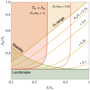
Figure 3: Excluded (shaded) regions in the plane of $\Lambda_{b}/\Lambda_{r}$ versus $f/\Lambda_{r}$. “Landscape” region violates condition (4); “Long Inflation” region violates condition (22); “Stability” denotes the vacuum stability bound (16); “$H_{I}$ range” curve denotes the limit beyond which the interval of allowed inflationary Hubble rates ${\cal H}_{I}$ from (13) vanishes. The dashed diagonal lines indicate the lowest allowed value of ${\cal H}_{I}/\Lambda_{r}$ in this allowed range as the axion mass is varied (see text). The bounds corresponding to “$T_{R}<\Lambda_{b}$” depend upon $\Lambda_{r}/m_{P}$ and are shown for two values of that ratio.

IV Vacuum stability

For our own $a$-vacuum to be habitable, it must not decay too quickly through tunneling to neighboring axionic vacua (not to be confused with the possible decay along the Higgs direction). This might occur during inflation, after reheating, when the effect of finite temperature is important, or at late times when we can consider $T$ to be zero.

At zero temperature, the criterion for vacuum stability becomes

$$Ae^{-S_{4}}\lesssim{\cal H}_{0}^{4}$$ (16)

where ${\cal H}_{0}$ is the present Hubble constant ($\sim e^{-140}m_{P}$ in Planckian units). $S_{4}$ is the 4D Euclidean action for critical bubbles corresponding to transitions between neighboring vacua Coleman:1977py . In (16), the prefactor $A=(S_{4}/2\pi)^{2}J$, with $J$ being a ratio of functional determinants with dimensions of [mass]⁴. The $J$ factor is difficult to compute, but is expected to be of order $\Lambda_{b}^{4}$ or $f^{4}$, always smaller than $\Lambda^{4}$ and $m_{P}^{4}$, so it is conservative to require $S_{4}\gtrsim 560$ as a condition for vacuum stability. We numerically compute the bounce solution and resulting $S_{4}$ and plot this stability condition, labeled “Stability,” in Figure 3.

An analytic formulation of the stability criterion can be obtained using the thin-wall approximation Coleman:1977py , in which the 4D action is

$$S_{4,tw}\simeq{27\pi^{2}\over 2}\,{\sigma^{4}\over\Delta V^{3}}\ ,$$ (17)

depending upon the bubble wall tension

$$\sigma\simeq\int_{0}^{2\pi f}da\,\sqrt{2\Lambda_{b}^{4}[1-\cos(a/f)]}=8\Lambda_{b}^{2}f\ ,$$ (18)

and the potential difference between neighboring vacua as given by (11). By numerical calculation of the actual tunneling action, we find that this approximation is not very good in the region of parameter space of interest; however by comparing the exact and approximate results it is possible to correct for this. The relevant parameter determining how well the thin-wall approximation works is $\Lambda_{b}/\Lambda_{r}$,   and we find that the fractional error in the action can be accurately fit to the formula

$$1-{S_{4}\over S_{4,tw}}\simeq 7.1\times 10^{-5}\left(\Lambda_{b}\over\Lambda_{r}\right)^{-7.845}$$ (19)

where $S_{4}$ is the full numerical value. This function is shown in fig. 4.

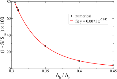
Figure 4: Fractional error in the thin-wall approximation for the 4D tunneling action, as a function of $\Lambda_{b}/\Lambda_{r}$. The analytic fit (19) as well as the numerical results are shown.

In the case of vacuum transitions due to thermal excitation over the barrier, one should estimate the 3D action for critical bubbles, taking also into account the thermal corrections to the potential. This is not a straightforward task: it depends on possible couplings of $a$ to other sectors of the theory and is limited to temperatures well below the critical temperature $T_{c}$ above which the dynamics responsible for the nonperturbative generation of the barriers in the axion potential become ineffective, but this is unspecified in our scenario. If the reheating temperature $T_{R}$ is above $T_{c}$ one expects the effective temperature-dependent barrier height $\Lambda_{b}^{4}(T)$ to start falling as a power of $T$ Preskill:1982cy . Given the level of uncertainty on $T_{c}$, we content ourselves with imposing the condition that $T_{R}<T_{c}\sim\Lambda_{b}$, as a rough estimate for $T_{c}$.

To obtain $T_{R}$ we use the relation for the Hubble parameter during radiation domination ${\cal H}_{R}=0.33\,\sqrt{g_{*}}\,T_{R}^{2}/m_{P}$. Assuming instant reheating we have ${\cal H}_{R}={\cal H}_{I}$ with ${\cal H}_{I}$ respecting (13), which translates into the range

$$0.54\frac{\sqrt{m_{a}m_{P}}}{\Lambda_{r}}<\frac{T_{R}}{\Lambda_{r}}\left(\frac{g_{*}}{g_{*}^{\rm SM}}\right)^{1/4}<0.56\sqrt{\frac{m_{P}}{\Lambda_{r}}}\ ,$$ (20)

with $g_{*}^{\rm SM}=106.75$. We exclude a point in parameter space if the lower limit of this range is bigger than $\Lambda_{b}/\Lambda_{r}$. The resulting limit is shown in Fig. 3, labeled $T_{R}<\Lambda_{b}$, for two representative values of $\Lambda_{r}/m_{P}=0.5,\,1$.

In cases (1) and (2) we must also consider the possibility of vacuum decay along the Higgs field direction, since we end up in the metastable region with respect to such decays. Metastability here means that quantum fluctuations at zero temperature are slow on the time scale ${\cal H}_{0}^{-1}$, and it does not take into account the possibility that tunneling was triggered at an earlier time by inflation. In fact during inflation, if $\cal{H}_{I}$ is higher than the instability scale, the Higgs field can be pushed over the barrier that separates the electroweak vacuum from the unstable region of field space EGR ; Zurek ; Higgstory , and this leads to an upper bound on ${\cal H}_{I}\sqrt{N_{e}}$, where $N_{e}$ is the number of e-folds. As discussed in the next section, this kind of bound can be generically violated in our framework if a very long period of inflation is needed to guarantee that the stationary solution to the Fokker-Planck equation is reached. In fact, this is the vacuum selection mechanism in case (3).

For cases (1) and (2) we then have to forbid such decays during inflation. A simple way of circumventing this danger is to have a nonminimal coupling $\xi|H|^{2}R$ between the Higgs field and the Ricci scalar $R$ EGR . During inflation, $R=-12{\cal H}_{I}^{2}$, and this provides a contribution $12\xi{\cal H}_{I}^{2}$ to the squared Higgs mass, that stabilizes the potential or suppresses Higgs fluctuations altogether (for $\xi>3/16$), relaxing the bound on ${\cal H}_{I}\sqrt{N_{e}}$ Higgstory . Subsequent to inflation, during preheating the induced Higgs mass term oscillates along with the inflaton, and this can cause parametric resonant production of Higgses, whose associated classical field can probe the instability region again preheatdec ; Dani and trigger vacuum decay. To avoid this, it is sufficient to have $\xi$ in the range $(0.06-4)$ Dani , which we assume to be the case for scenarios (1) and (2).

V Initial conditions

We have assumed that the stationary solution of the Fokker-Planck equation was achieved during inflation. Here we consider how long a period of inflation would be required to achieve this, starting from some different initial condition, for example that $P(a)$ was peaked around the true vacuum state. The barriers between neighboring vacua must be large enough to prevent tunneling at late times, while the scale of inflation must be sufficiently low so that $P(a)$ is not too flat, eq. (10). Both of these tend to slow the time evolution of $P$.

It is instructive to consider a toy model consisting of a double-well potential $V(\phi)$ with just two vacuum states, separated by a barrier height $V_{b}$ that is large compared to the energy difference between the two vacua. The system is initially sharply localized in one of the vacua, $\phi_{1}$, and allowed to evolve in time according to the Fokker-Planck equation. By a combination of numerical and analytical methods one discovers two relevant time scales, hierarchically different. The shorter one, $\tau_{1}\simeq 3{\cal H}_{I}/[2V^{\prime\prime}(\phi_{1})]$, is associated with the spread of $P$ until it reaches an approximately Gaussian shape around the starting vacuum, $P(\phi)\simeq\exp[-(\phi-\phi_{1})^{2}/(2\sigma_{1}^{2})]$, with $\sigma_{1}^{2}=3{\cal H}_{I}^{4}/[8\pi^{2}V^{\prime\prime}(\phi_{1})]$. This solution is valid for small displacements and is quasi-stationary. The long time scale, $\tau_{t}$, is associated with the probability leakage to the second vacuum at $\phi_{2}$, through the top of the barrier, at $\phi_{t}$. The associated rate, $\Gamma=1/\tau_{t}$, is

$$\Gamma\sim{{\cal H}_{I}^{3}\over 16\pi^{2}\sigma_{1}\sigma_{t}}\,e^{-8\pi^{2}V_{b}/3{\cal H}_{I}^{4}}\ ,$$ (21)

where $\sigma_{t}^{2}=3{\cal H}_{I}^{4}/(8\pi^{2}|V^{\prime\prime}(\phi_{t})|)$.

Applying this estimate to our scenario, we see that to avoid an exponentially long period of inflation, one needs ${\cal H}_{I}^{4}\gtrsim 8\pi^{2}V_{b}/3$, while condition (10) implies ${\cal H}_{I}^{4}\lesssim 8\pi^{2}\Delta\overline{V}/3$. Using $V_{b}=\Lambda_{b}^{4}$ and $\Delta\overline{V}$ from (11), the combined conditions require

$$\Lambda_{b}/\Lambda_{r}<0.47\ .$$ (22)

Hence it is possible to satisfy all the criteria without having a very long period of inflation.

However, a more generic situation is to admit a prior period of eternal inflation, which would automatically justify the stationary solution since then an arbitrarily long period of evolution could occur prior to the final stage of observable inflation. Two common situations can admit eternal inflation. First, inflation could be chaotic during the primordial stage, with the inflaton displaced high enough on its potential so that upward quantum fluctuations can dominate over the classical downhill evolution LindeEternal . Second, the inflaton (not necessarily the same inflaton that is responsible for the final stage of inflation) could be trapped in a false vacuum with an exponentially long lifetime, the exponential of the tunneling action LinVil . Either case allows us to relax the requirement (22).

VI Summary and conclusions

We have presented a concrete realization of a mechanism to explain the near-criticality of the SM Higgs quartic coupling $\lambda$. It uses an axion-like field $a$ with a potential that develops a large number of non-degenerate vacua in which $\lambda$ takes different values, effectively scanning, due to a coupling of the Higgs to $a$. The vacua are assumed to be populated during inflation with probabilities that depend exponentially on the ratio $V(a)/{\cal H}_{I}^{4}$. By appropriately choosing the sign of the overall slope of $V(a)$, vacua with increasingly negative values of $\lambda$ are favored. The conditional probability for a particular vacuum state given that it is compatible with observers, is zero if it undergoes catastrophic decay of the Higgs vacuum. Thus the most likely anthropically allowed states are those that are close to a critical line in the plane of $\lambda$ and $y_{t}$. We discussed three different scenarios, summarized in Table 1 and illustrated by Fig. 2. They require different cosmological histories and parameters for the potential of the $a$ field, and they depend upon the precise value of the top quark mass.

In case (1), vacua beyond the instability line are depleted by quantum tunneling, which is faster than the age of the universe. In case (2), that requires a large reheating temperature, thermal fluctuations over the Higgs barrier remove vacua beyond the thermal instability line. In case (3), which requires a high inflationary Hubble rate or a large number of e-folds, Higgs fluctuations induced during inflation trigger vacuum decay along the unstable Higgs direction, effectively selecting vacua with stable Higgs potentials.

While the mechanism we have discussed offers an explanation for the intriguing near-criticality of the Higgs quartic coupling, it does not address the hierarchy problem. It would be quite interesting to find a mechanism that could address both issues simultaneously, especially given the fact that similar mechanisms (e.g. relaxions) offer potential solutions to the hierarchy problem.

It is perhaps disappointing that this scenario does not make positive predictions for new physics at experimentally accessible energies. Since the only new field, the axion, has a mass {typically much larger than the electroweak scale, there are no manifestations at low energy. Instead, we predict an absence of new physics coupling to the Higgs field at low scales, to the extent that such couplings would move the critical lines of stability away from their standard model values. On the other hand, we think it is interesting that despite the lack of low-energy experimental tests, the mechanism is highly constrained by considerations of theoretical and cosmological consistency. It shows that the mere existence of a landscape is not sufficient for a successful anthropic explanation of tuning problems. Our results further indicate that the new physics scale should generically be very high (not far below the string or Planck scale) to make the vacua of the landscape stable against tunneling both during inflation and at late times, and that a prior period of eternal inflation is strongly motivated.

Acknowledgments. J.M.C. thanks A. Linde, L. McAllister and M. Trott for helpful discussions, and the CERN Theory Department and Niels Bohr International Academy for hospitality while this work was in progress, which was also supported by the Natural Sciences and Engineering Research Council of Canada. The work of J.R.E. has been partly supported by the ERC grant 669668 – NEO-NAT – ERC-AdG-2014, the Spanish Ministry MINECO under grants 2016-78022-P and FPA2014-55613-P, the Severo Ochoa excellence program of MINECO (grant SEV-2016-0588) and by the Generalitat grant 2014-SGR-1450.

References

- (1) G. Degrassi, S. Di Vita, J. Elias-Miro, J.R. Espinosa, G.F. Giudice, G. Isidori and A. Strumia, “Higgs mass and vacuum stability in the Standard Model at NNLO,” JHEP 1208, 098 (2012) [hep-ph/1205.6497]; D. Buttazzo, G. Degrassi, P.P. Giardino, G.F. Giudice, F. Sala, A. Salvio and A. Strumia, “Investigating the near-criticality of the Higgs boson,” JHEP 1312 (2013) 089 [hep-ph/1307.3536].
- (2) M.R. Douglas, “The Statistics of string/M theory vacua,” JHEP 0305, 046 (2003) [hep-th/0303194].
- (3) S. Ashok and M.R. Douglas, “Counting flux vacua,” JHEP 0401, 060 (2004) [hep-th/0307049].
- (4) A.D. Linde, “Eternal Chaotic Inflation,” Mod. Phys. Lett. A 1, 81 (1986); “Eternally Existing Selfreproducing Chaotic Inflationary Universe,” Phys. Lett. B 175, 395 (1986).
- (5) R. Bousso and J. Polchinski, “Quantization of four form fluxes and dynamical neutralization of the cosmological constant,” JHEP 0006, 006 (2000) [hep-th/0004134].
- (6) S. Weinberg, “Anthropic Bound on the Cosmological Constant,” Phys. Rev. Lett. 59, 2607 (1987).
- (7) S.R. Coleman, “Why There Is Nothing Rather Than Something: A Theory of the Cosmological Constant,” Nucl. Phys. B 310, 643 (1988).
- (8) V.A. Rubakov and M.E. Shaposhnikov, “A Comment on Dynamical Coupling Constants and the Anthropic Principle,” Mod. Phys. Lett. A 4, 107 (1989).
- (9) N. Cabibbo, L. Maiani, G. Parisi and R. Petronzio, “Bounds on the Fermions and Higgs Boson Masses in Grand Unified Theories,” Nucl. Phys. B 158, 295 (1979). P.Q. Hung, “Vacuum Instability and New Constraints on Fermion Masses,” Phys. Rev. Lett. 42, 873 (1979);
- (10) M. Lindner, M. Sher and H.W. Zaglauer, “Probing Vacuum Stability Bounds at the Fermilab Collider,” Phys. Lett. B 228, 139 (1989); M. Sher, “Electroweak Higgs Potentials and Vacuum Stability,” Phys. Rept. 179 (1989) 273; P.B. Arnold, “Can the Electroweak Vacuum Be Unstable?,” Phys. Rev. D 40 (1989) 613; G. Altarelli and G. Isidori, “Lower limit on the Higgs mass in the standard model: An Update,” Phys. Lett. B 337 (1994) 141; J.A. Casas, J.R. Espinosa and M. Quirós, “Standard model stability bounds for new physics within LHC reach,” Phys. Lett. B 382 (1996) 374 [hep-ph/9603227]; T. Hambye and K. Riesselmann, “Matching conditions and Higgs mass upper bounds revisited,” Phys. Rev. D 55 (1997) 7255 [hep-ph/9610272]; G. Isidori, G. Ridolfi and A. Strumia, “On the metastability of the standard model vacuum,” Nucl. Phys. B 609 (2001) 387 [hep-ph/0104016]; J. Ellis, J.R. Espinosa, G.F. Giudice, A. Hoecker and A. Riotto, “The Probable Fate of the Standard Model,” Phys. Lett. B 679 (2009) 369 [hep-ph/0906.0954]; F. Bezrukov, M.Y. Kalmykov, B.A. Kniehl and M. Shaposhnikov, “Higgs Boson Mass and New Physics,” JHEP 1210 (2012) 140 [hep-ph/1205.2893]; J. Elias-Miró, J.R. Espinosa, G.F. Giudice, G. Isidori, A. Riotto and A. Strumia, “Higgs mass implications on the stability of the electroweak vacuum,” Phys. Lett. B 709 (2012) 222 [hep-ph/1112.3022]; A.V. Bednyakov, B.A. Kniehl, A.F. Pikelner and O.L. Veretin, “Stability of the Electroweak Vacuum: Gauge Independence and Advanced Precision,” Phys. Rev. Lett. 115 (2015) 201802 [hep-ph/1507.08833].
- (11) J.R. Espinosa, “Vacuum Stability and the Higgs Boson,” PoS LATTICE 2013 (2014) 010 [hep-lat/1311.1970].
- (12) B. Feldstein, L.J. Hall and T. Watari, “Landscape Prediction for the Higgs Boson and Top Quark Masses,” Phys. Rev. D 74 (2006) 095011 [hep-ph/0608121].
- (13) L. McAllister, E. Silverstein and A. Westphal, “Gravity Waves and Linear Inflation from Axion Monodromy,” Phys. Rev. D 82, 046003 (2010) [hep-th/0808.0706]; L. McAllister, P. Schwaller, G. Servant, J. Stout and A. Westphal, “Runaway Relaxion Monodromy,” [hep-th/1610.05320].
- (14) P.W. Graham, D.E. Kaplan and S. Rajendran, “Cosmological Relaxation of the Electroweak Scale,” Phys. Rev. Lett. 115 (2015) 22, 221801 [hep-ph/1504.07551].
- (15) D.E. Kaplan and R. Rattazzi, “Large field excursions and approximate discrete symmetries from a clockwork axion,” Phys. Rev. D 93 (2016) 085007 [hep-ph/1511.01827]; K. Choi and S.H. Im, “Realizing the relaxion from multiple axions and its UV completion with high scale supersymmetry,” JHEP 1601 (2016) 149 [hep-ph/1511.00132].
- (16) Liam McAllister, private communication.
- (17) J. Elias-Miró, J.R. Espinosa, G.F. Giudice, G. Isidori, A. Riotto and A. Strumia, “Higgs mass implications on the stability of the electroweak vacuum,” Phys. Lett. B 709, 222 (2012) [hep-ph/1112.3022].
- (18) [ATLAS and CDF and CMS and D0 Collaborations], “First combination of Tevatron and LHC measurements of the top-quark mass,” [hep-ex/1403.4427].
- (19) A. Salvio, A. Strumia, N. Tetradis and A. Urbano, “On gravitational and thermal corrections to vacuum decay,” JHEP 1609 (2016) 054 [hep-ph/1608.02555].
- (20) J.R. Espinosa, G.F. Giudice, E. Morgante, A. Riotto, L. Senatore, A. Strumia and N. Tetradis, “The cosmological Higgstory of the vacuum instability,” JHEP 1509 (2015) 174 [hep-ph/1505.04825].
- (21) G. Aad et al. [ATLAS and CMS Collaborations], “Combined Measurement of the Higgs Boson Mass in Collisions at and 8 TeV with the ATLAS and CMS Experiments,” Phys. Rev. Lett. 114 (2015) 191803 [hep-ex/1503.07589].
- (22) A.D. Linde, “Hard art of the universe creation (stochastic approach to tunneling and baby universe formation),” Nucl. Phys. B 372 (1992) 421 [hep-th/9110037].
- (23) J.R. Espinosa, G.F. Giudice and A. Riotto, “Cosmological implications of the Higgs mass measurement,” JCAP 0805 (2008) 002 [hep-ph/0710.2484].
- (24) A. Hook, J. Kearney, B. Shakya and K.M. Zurek, “Probable or Improbable Universe? Correlating Electroweak Vacuum Instability with the Scale of Inflation,” JHEP 1501 (2015) 061 [hep-ph/1404.5953]; J. Kearney, H. Yoo and K.M. Zurek, “Is a Higgs Vacuum Instability Fatal for High-Scale Inflation?,” Phys. Rev. D 91 (2015) no.12, 123537 [hep-th/1503.05193]; W.E. East, J. Kearney, B. Shakya, H. Yoo and K.M. Zurek, “Spacetime Dynamics of a Higgs Vacuum Instability During Inflation,” Phys. Rev. D 95 2, 023526 (2017) [hep-ph/1607.00381].
- (25) A.D. Linde, private communication.
- (26) S.R. Coleman, “The Fate of the False Vacuum. 1. Semiclassical Theory,” Phys. Rev. D 15, 2929 (1977) Erratum: [Phys. Rev. D 16, 1248 (1977)].
- (27) J. Preskill, M.B. Wise and F. Wilczek, “Cosmology of the Invisible Axion,” Phys. Lett. 120B, 127 (1983).
- (28) M. Herranen, T. Markkanen, S. Nurmi and A. Rajantie, “Spacetime curvature and Higgs stability after inflation,” Phys. Rev. Lett. 115 (2015) 241301 [hep-ph/1506.04065]; Y. Ema, K. Mukaida and K. Nakayama, “Fate of Electroweak Vacuum during Preheating,” [hep-ph/1602.00483]; K. Kohri and H. Matsui, “Higgs vacuum metastability in primordial inflation, preheating, and reheating,” [hep-ph/1602.02100]; K. Enqvist, M. Karciauskas, O. Lebedev, S. Rusak and M. Zatta, “Postinflationary vacuum instability and Higgs-inflaton couplings,” JCAP 1611 (2016) 025 [hep-ph/1608.08848]; M. Postma and J. van de Vis, “Electroweak stability and non-minimal coupling,” JCAP 1705 (2017) 004 [hep-ph/1702.07636]; Y. Ema, M. Karciauskas, O. Lebedev and M. Zatta, “Early Universe Higgs dynamics in the presence of the Higgs-inflaton and non-minimal Higgs-gravity couplings,” [hep-ph/1703.04681].
- (29) D.G. Figueroa, A. Rajantie and F. Torrenti, “Higgs-curvature coupling and post-inflationary vacuum instability,” [astro-ph.CO/1709.00398].
- (30) A.D. Linde, “The New Inflationary Universe Scenario,” In Cambridge 1982, Proceedings, The Very Early Universe, 205-249; A. Vilenkin, “The Birth of Inflationary Universes,” Phys. Rev. D 27, 2848 (1983).