5-brane webs for 5d $\mathcal{N}=1$ $G_{2}$ gauge theories

Abstract

We propose 5-brane webs for 5d $\mathcal{N}=1$ $G_{2}$ gauge theories. From a Higgsing of the $SO(7)$ gauge theory with a hypermultiplet in the spinor representation, we construct two types of 5-brane web configurations for the pure $G_{2}$ gauge theory using an O5-plane or an $\widetilde{\text{O5}}$-plane. Adding flavors to the 5-brane web for the pure $G_{2}$ gauge theory is also discussed. Based on the obtained 5-brane webs, we compute the partition functions for the 5d $G_{2}$ gauge theories using the recently suggested topological vertex formulation with an O5-plane, and we find agreement with known results.

1 Introduction

5-brane webs in type IIB string theory have been used to study five-dimensional (5d) superconformal field theories (SCFTs) that are ultraviolet (UV) completions of a certain class of 5d $\mathcal{N}=1$ supersymmetric gauge theories Seiberg:1996bd ; Morrison:1996xf ; Douglas:1996xp ; Intriligator:1997pq ; Aharony:1997ju ; Aharony:1997bh . A 5-brane web configuration provides us with a tool to compute the instanton partition function that captures the BPS spectrum of a 5d theory realized on a 5-brane web as well as with a perspective of qualitative understandings of the SCFTs such as global symmetry enhancements and various dualities.

By introducing an orientifold plane like an O7-plane or an O5-plane, 5-brane webs can be enriched so that one can describe 5d theories with some other classical gauge group, such as $SO(N),USp(2N)$ Brunner:1997gk ; Bergman:2015dpa ; Hayashi:2015vhy ; Zafrir:2015ftn , in addition to the standard classical gauge group $SU(N)$. In recent years there has been some progress on brane configurations with the orientifold planes. For example, in Hayashi:2015zka ; Hayashi:2016abm ; Yun:2016yzw , whether we resolve an O7^--plane into two $[p,q]$ 7-branes or not in a certain 5-brane web configuration gives an explanation for equivalence proposed in Gaiotto:2015una of two theories at the UV fixed point, an $SU(N+1)$ theory with $N_{f}\leq 2N+6$ hypermultiplets in the fundamental representation (flavors) and the Chern-Simons (CS) level $\kappa=\pm\left(N+3-N_{f}/2\right)$, and an $USp(2N)$ theory with the same number of flavors. In particular, it has been discussed in Zafrir:2015ftn ; Zafrir:2016jpu that 5-brane configurations with an O5-plane can realize an $SO(N)$ gauge theory even with hypermultiplets in the spinor/conjugate spinor representation. It is also noticeable that one can differentiate the discrete theta angle ($\theta=0,\pi$) of the 5d pure $USp(2N)$ gauge theory Morrison:1996xf ; Douglas:1996xp ; Intriligator:1997pq from 5-brane webs with an O5-plane. The two different theta angles turn out to imply two distinct phase structures for their 5-brane webs, that are characterized by two distinct “generalized” flop transitions which may be applied to 5-branes intersecting at the same point with an O5-plane Hayashi:2017btw .

There has been also progress along a quantitative side on 5-brane webs with an O5-plane. The conventional topological vertex formalism Aganagic:2003db ; Iqbal:2007ii ; Awata:2008ed enables one to systematically compute the Nekrasov instanton partition function of a 5d theory on a 5-brane web via the correspondence Leung:1997tw between a toric diagram and a certain $(p,q)$ 5-brane web diagram. Although 5-brane webs for $SU(N)$ gauge theories with a large number of flavors or a large CS level often lead to non-toric Calabi-Yau geometries Benini:2009gi , the topological vertex formulation is still applicable to reproduce the correct partition function Hayashi:2013qwa ; Hayashi:2014wfa ; Hayashi:2015xla ; Kim:2015jba ; Hayashi:2016abm ; Hayashi:2016jak . Quite recently, the topological vertex formulation has been further extended to 5-brane webs with an O5-plane Kim:2017jqn . Together with a generalized flop transition, the new method utilizes a configuration where one-half of the original brane configuration is glued to the other half from the mirror image due to an O5-plane in a specific manner.

The purpose of this paper is to further extend the study of 5-brane webs with an O5-plane and propose 5-brane web diagrams for 5d $\mathcal{N}=1$ gauge theories of an exceptional gauge group $G_{2}$, using these recent developments on 5-brane webs. We then compute their Nekrasov partition functions based on the topological vertex formalism for 5-brane webs with an O5-plane.

Our strategy is as follows: A 5-brane web diagram for the $SO(7)$ gauge theory with a hypermultiplet in the spinor representation has been constructed in Zafrir:2015ftn . We then consider the Higgs branch of the $SO(7)$ gauge theory with one spinor in terms of the web diagram, which should yield a 5-brane web configuration for the pure $G_{2}$ gauge theory.

We note that there are two ways to obtain the web diagram for the $SO(7)$ gauge theory with one spinor. One way is to Higgs the $SO(8)$ gauge theory with a hypermultiplet in the vector representation and a hypermultiplet in the spinor or conjugate spinor representation. The other way is to Higgs the $SO(8)$ gauge theory with a hypermultiplet in the spinor representation and a hypermultiplet in the conjugate spinor representation. These two $SO(8)$ gauge theories should be equivalent to each other due to the triality of $SO(8)$, and both Higgsings hence give rises to the $SO(7)$ gauge theory with one spinor, while the resulting brane configurations look different. Further Higgsing of the two types of the diagrams leads to two different 5-brane webs for the pure $G_{2}$ gauge theory, which therefore gives two different configuration for the same $G_{2}$ gauge theory. It is possible to add flavors to the pure $G_{2}$ gauge theory by Higgsing the $SO(7)$ gauge theory with hypermultiplets either in the vector representation or the spinor representation in addition to one spinor. We test our proposal by comparing the area of compact faces that a D3-brane wraps on the 5-brane webs with the tension of a monopole string which can be calculated from the effective prepotential of the theory in question. In fact the analysis implies an interesting feature like which faces of a 5-brane web a D3-brane wraps in the presence of an O5-plane.

We then go on to compute the Nekrasov partition function for 5d $\mathcal{N}=1$ $G_{2}$ gauge theories by applying the recently proposed topological vertex method for 5-brane webs with an O5-plane Kim:2017jqn . We check that our partition function for the pure $G_{2}$ gauge theory reproduces the one-instanton result Benvenuti:2010pq ; Keller:2011ek and also the two-instanton result Hanany:2012dm ; Keller:2012da ; Cremonesi:2014xha . We also show that the partition function of the $G_{2}$ gauge theory with one flavor is consistent with flavor decoupling.

The paper is organized as follows: In section 2, we first discuss a 5-brane web for the $SO(7)$ gauge theory with a hypermultiplet in the spinor representation. By Higgsing the $SO(7)$ theory with one spinor, we propose a 5-brane web for the pure $G_{2}$ gauge theory. We check that the proposed diagram is consistent with the effective prepotential of the pure $G_{2}$ gauge theory. We also present two ways to introduce flavors. In section 3, using the triality of $SO(8)$ gauge theory among hypermultiplets in the vector, spinor, and conjugate spinor representations, we propose another 5-brane web for the pure $G_{2}$ theory through successive Higgsings of the $SO(8)$ gauge theory theory with one spinor and one conjugate spinor. In section 4, we first review a recent proposal for the topological vertex formulation with an O5-plane and extend it to the cases with an $\widetilde{\text{O5}}$-plane. We then use it to compute the partition functions of 5d $\mathcal{N}=1$ $G_{2}$ gauge theories with no flavor and with one flavor. In section 5, we summarize the results and comment on further directions.

Note added: We are informed that the authors of Kim:2018gjo computed the partition function for 5d $\mathcal{N}=1$ $G_{2}$ gauge theories using the ADHM-like method, which will appear in arXiv.

2 $G_{2}$ gauge theories from an $\widetilde{\text{O5}}$-plane

In string theory, a wide class of 5d theories with eight supercharges can be constructed by $(p,q)$ 5-brane webs in type IIB string theory Aharony:1997ju ; Aharony:1997bh ; Leung:1997tw or M-theory on Calabi-Yau threefolds Morrison:1996xf ; Douglas:1996xp ; Intriligator:1997pq . We will make use of the 5-brane web description for constructing 5d $\mathcal{N}=1$ gauge theories in this paper. In this section, we present 5-brane web diagrams which realize 5d $G_{2}$ gauge theories by using an $\widetilde{\text{O5}}$-plane. Although D5-branes on top of an O5-plane or an $\widetilde{\text{O5}}$-plane usually generate an $SO/USp$ gauge theory, we will argue that some simple 5-brane web diagram with an $\widetilde{\text{O5}}$-plane can yield a 5d $G_{2}$ gauge theory in an intriguing way.

2.1 $SO(7)$ gauge theory with spinor matter

Before constructing 5-brane webs for $G_{2}$ gauge theories, we first discuss 5-brane web realization of $SO(7)$ gauge theories using an $\widetilde{\text{O5}}$-plane in this subsection. By using this construction, we will see in section 2.2 that a Higgsing of the 5-brane web diagrams of the $SO(7)$ gauge theories with a hypermultiplet in spinor representation can generate 5-brane webs for the pure $G_{2}$ gauge theory.

A 5-brane web diagram for the pure $SO(7)$ gauge theory can be realized using an $\widetilde{\text{O5}}$-plane. Naively, a 5-brane web with an $\widetilde{\text{O5}}$-plane may look problematic since the difference of the RR charge between an $\widetilde{\text{O5}}^{+}$-plane and an $\widetilde{\text{O5}}^{-}$-plane is fractional, which implies the appearance of $(p,q)$ 5-branes with non-integer $p$. A way out is that an $\widetilde{\text{O5}}$-plane may be thought of as an O5-plane with a half monodromy branch cut associated to a half D7-brane Zafrir:2015ftn . Namely, an effective description of an $\widetilde{\text{O5}}^{-}$-plane is an O5^--plane and a half D5-brane plus the half monodromy cut. An $\widetilde{\text{O5}}^{+}$-plane is also effectively described by an O5⁺-plane plus the half monodromy cut. Since the monodromy created by this cut is half of the original monodromy associated to one full D7-brane, it changes the potential fractional charge to integer charge.

The web diagram for the pure $SO(7)$ gauge theory can be derived by a Higgsing of the $SO(8)$ gauge theory with a hypermultiplet in the vector representation. Through this process, we will see that the $\widetilde{\text{O5}}$-plane is accompanied by the half monodromy cut. A 5-brane web diagram of the $SO(8)$ gauge theory with one flavor is constructed with O5^--plane as given in Figure 1.

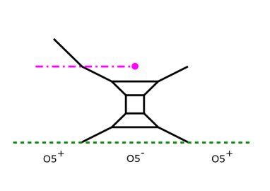
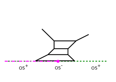
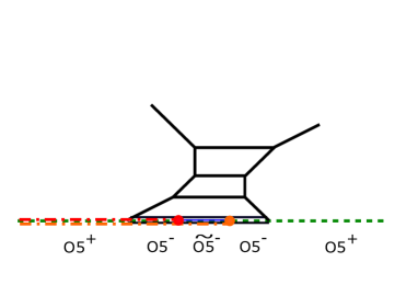
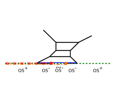
Figure 1: A Higgsing procedure of the 5-brane web of the $SO(8)$ gauge theory with one flavor to the 5-brane web of the pure $SO(7)$ gauge theory. (a): Moving the flavor D7-brane to the middle of the diagram. The branch cut is denoted by the dashed line. (b): Lowering the flavor D7-brane as well as the bottom color D5-brane to the O5^--plane. (c): Splitting the D7-branes into two half D7-branes. We have an $\widetilde{\text{O5}}^{-}$-plane between the half D7-branes and there are effectively three fractional D5-branes between the half D7-branes. We also have monodromy branch cuts for the half D7-branes represented by the red and orange dashed lines. (d): Removing the two fractional D5-branes. We have a half D5-brane denoted by the blue line stretched between the $(2,1)$ 5-brane and the $(1,-1)$ 5-brane. The diagram gives the pure $SO(7)$ gauge theory.

We put a floating D7-brane to realize one flavor and we put the branch cut associated with this D7-brane in the left direction. Note that $(p,q)$ charges of the 5-branes change when they go across this cut. In order to perform the Higgsing, we lower this D7-brane as well as the bottom color D5-brane to the position of the O5^--plane. Since the left part of the web diagram crosses the branch cut, the 5-brane charges change accordingly as in Figure 1.

On the O5^--plane, the D7-brane can be split into two half D7-branes, generating an $\widetilde{\text{O5}}^{-}$-plane in between Evans:1997hk ; Giveon:1998sr ; Feng:2000eq ; Bertoldi:2002nn . Counting the half D5-brane associated to the $\widetilde{\text{O5}}^{-}$-plane together with the bottom color D5-brane, we have effectively three half D5-branes between these two half D7-branes. Note also that half monodromy cut appears between the two half D7-branes. The 5-brane web after the splitting is depicted in Figure 1.

At this stage, it is possible to move the two half D5-branes between the half D7-branes off the plane of the 5-brane web, which degree of freedom corresponds to the one-dimensional Higgs branch. Thus, removing the two half D5-branes infinitely far away should correspond to the Higgsing of the $SO(8)$ gauge theory with one flavor down to the pure $SO(7)$ gauge theory. After removing the two half D5-branes, we see that one half D5-brane stretch between the $(2,1)$ 5-brane and the $(1,-1)$ 5-brane including the one coming from the $\widetilde{\text{O5}}^{-}$-plane. In addition, we have one half D5-brane connecting the $(2,1)$ 5-brane to the left half D7-brane and also another half D5-brane connecting the $(1,-1)$ 5-brane to the right half D7-brane as in Figure 1, which configuration preserves the s-rule.

Although the 5-brane web diagram in Figure 1 still has an remaining O5-plane, one can change it into an $\widetilde{\text{O5}}^{-}$-plane by moving the left/right half D7-brane to infinitely left/right respectively. No half D5-branes are attached to the half D7-branes after they go across the $(2,1)$ 5-brane or $(1,-1)$ 5-brane due to Hanany-Witten effect Hanany:1996ie . Note that the half monodromy cut between the two half D7-brane still remains even after moving them to infinity. That is, we see that the $\widetilde{\text{O5}}$-plane is accompanied by the half monodromy cut. The 5-brane web diagram after moving the half D7-branes in the opposite directions is given in Figure 2. This is exactly the web diagram for the pure $SO(7)$ gauge theory, which have three color D5-branes with the $\widetilde{\text{O5}}^{-}$-plane.

Figure 2: Another 5-brane web diagram for the 5d pure $SO(7)$ gauge theory by removing the half D7-branes in the opposite directions. The diagram is constructed with an $\widetilde{\text{O5}}$-plane. The $\widetilde{\text{O5}}$-plane is realized by the O5-plane with the half monodromy cut which is denoted by the orange dashed line.

It is straightforward to include a hypermultiplet in the vector representation of $SO(7)$. The vector matter can be introduced by adding a flavor D5-brane to the 5-brane web diagram of the pure $SO(7)$ gauge theory. In fact, one can also introduce spinor matter to the 5-brane web of the $SO(7)$ gauge theory. From the 5-brane web viewpoint, the spinor matter can be realized non-perturbatively Zafrir:2015ftn . To see that, let us consider a 5-brane web diagram in Figure 3.

Figure 3: A 5-brane web diagram for the $[1]-SO(9)-USp(2)-\left[\frac{3}{2}\right]$ quiver theory.

The web diagram gives a $[1]-SO(9)-USp(2)-\left[\frac{3}{2}\right]$ quiver theory. Here $[n]-G$ stands for $n$ flavors attached to the $G$ gauge theory. The quiver theory has a Higgs branch associated to moving a D5-brane off the plane of the 5-brane web. The Higgsing yields a 5-brane web diagram given in Figure 4.

Figure 4: A 5-brane web diagram for a $SO(7)$ gauge theory with spinor matter obtained by removing the D5-brane from the diagram for the $[1]-SO(9)-USp(2)-\left[\frac{3}{2}\right]$ quiver theory.

The resulting theory might naively look like the pure $SO(7)$ gauge theory. However, the gauge coupling of the “$USp(0)$” gauge group is not still turned off. We may expect some additional degrees of freedom whose mass is the inverse of the gauge coupling. In other words, the 5-brane web appears to have “$USp(0)$” instantons. Before the Higgsing, we indeed have $USp(2)$ instantons and the instantons carry charges in the spinor representation of $SO(9)$. Hence, after the Higgsing, a natural candidate for the “$USp(0)$” instantons is a hypermultiplet in the spinor representation of the $SO(7)$ gauge theory. Namely, the 5-brane web in Figure 4 gives rise to an $SO(7)$ gauge theory with a hypermultiplet in the spinor representation.

2.2 5-brane web for pure $G_{2}$ gauge theory

We then move on to construct a 5-brane web diagram for a pure $G_{2}$ gauge theory. By Higgsing the $SO(7)$ gauge theory with one hypermultiplet in the spinor representation yields the pure $G_{2}$ gauge theory. Thus, the corresponding process in the 5-brane web diagram for the $SO(7)$ gauge theory with one spinor in Figure 4 should lead to the web diagram for the pure $G_{2}$ gauge theory. The web diagram in Figure 4 implies that the theory possesses an $SU(2)$ flavor symmetry associated to parallel external $(2,1)$ 5-branes. This global symmetry is expected to act on the hypermultiplet in the spinor representation. Thus, the distance of the two parallel external $(2,1)$ 5-branes should be associated to the mass of this spinor and the Higgs branch should open up in the massless limit at certain subspace in the Coulomb moduli. The question is how one can take the massless limit. It seems to be difficult take the massless limit from the diagram in Figure 4 since we need to “flop” the $\widetilde{\text{O5}}^{+}$-plane between the $(2,1)$ 5-brane and the $(1,-1)$ 5-brane.

In order to resolve the issue, it turns out to be useful to consider an equivalent but different 5-brane web diagram for the $SO(7)$ gauge theory with one spinor. Analogous to Figure 2 being obtained from Figure 1, the diagram in Figure 4 may be obtained by moving the two half D7-branes in the opposite directions from the diagram in Figure 5.

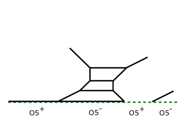
Figure 5: 5-brane web diagrams for the $SO(7)$ gauge theory with one spinor. (a): The 5-brane web diagram which is obtained by Higgsing the diagram of the $SO(8)$ gauge theory with one vector and one spinor. Compared to the diagram in Figure 1, the $(2,1)$ 5-brane is attached on the right, yielding the spinor matter. Removing the half D7-branes in the opposite direction gives the diagram in Figure 4. (b): An equivalent diagram to the one in Figure 5 (and also to the one in Figure 4). We move the half D7-branes in the left direction compared to the diagram in Figure 5. Then the monodromy cut disappears and the diagram is constructed with an O5-plane.

Instead, we can consider another deformation from the diagram in Figure 5 by moving both the half D7-branes to infinitely left. The resulting 5-brane web is depicted in Figure 5. After this deformation, the monodromy cuts completely disappears from the diagram and hence we have only an O5-plane. Therefore, a 5-brane web diagram with an $\widetilde{\text{O5}}$-plane has an equivalent 5-brane web diagram without an $\widetilde{\text{O5}}$-plane but with only an O5-plane. The transition is done by moving a half D7-brane from the infinitely right to the infinitely left in the diagram with an $\widetilde{\text{O5}}$-plane. We will make use of this transition in this paper.

By using this diagram, we can take the massless limit of the spinor by using “generalized flop transition” Hayashi:2017btw . Let us focus on the local part of the diagram describing the “$USp(0)$” gauge theory. On the left side a $(1,-1)$ 5-brane intersects with an O5-plane together with a full D5-brane. On the other hand, a $(2,1)$ 5-brane intersects with the O5-plane on the right side. The local structure exactly appears in the 5-brane diagram of the $E_{2}$ theory, and hence we can perform a generalized flop transition for this local part by using the results in Hayashi:2017btw . Through the process of studying the phase diagram of the $E_{2}$ theory, it is proposed that the diagram in Figure 6 is flopped either to the one in Figure 6 or Figure 6. Whether the diagram is flopped to the one in Figure 6 or Figure 6 is translated to the sign of the mass parameter of the $USp(0)$ gauge theory, which is the sign of the Coulomb branch parameter in our case. Although this transition is obtained for the $E_{2}$ theory, it is natural to assume that this transition is always available regardless of the detail of the remaining diagram to which this subdiagram is attached. On one hand, by considering a limit where the D5-brane comes down to the position of an O5-plane as we did in the process of the Higgsing, Figure 6 reduces to Figure 7, which corresponds to the one appearing in the local part of the diagram in Figure 5. On the other hand, by the same limit, Figure 6 and Figure 6 both reduce to Figure 7. Therefore, we propose that the $USp(0)$ part in Figure 5 can be flopped to the form in Figure 7.

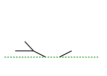
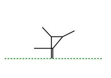
Figure 6: A generalized flop transition for a 5-brane web with an O5-plane. Whether the diagram in (a) is flopped to (b) or (c) depends on the sign of the mass parameter associated to the D5-brane.

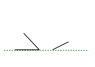
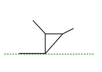
Figure 7: The generalized flop transition in Figure 6 in the case when the height of the D5-brane in Figure 6 is set to zero.

The equivalent flop transition in the presence of an $\widetilde{\text{O5}}$-plane is given in Figure 8.

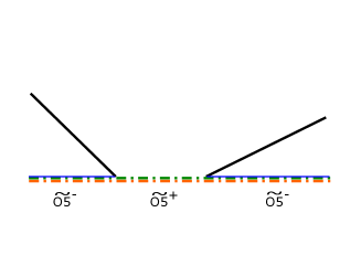
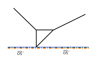
Figure 8: A generalized flop transition from (a) to (b) which is equivalent to the one in Figure 7.

After considering the transition in Figure 7 for the local $USp(0)$ part in Figure 5, the 5-brane web diagram becomes the one in Figure 9.

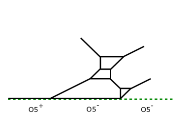
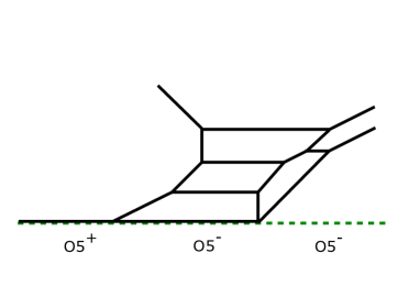
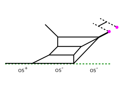
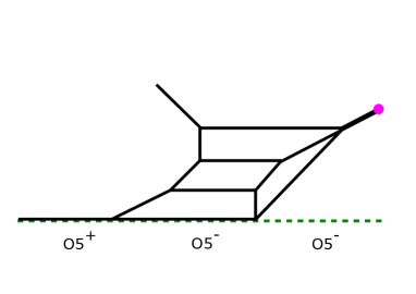
Figure 9: A Higgsing procedure which gives rise to a 5-brane web diagram for the pure $G_{2}$ gauge theory. (a): We performed the generalized flop transition compared to the diagram in Figure 5. (b): We performed two standard flop transitions to the diagram in Figure 9. (c): Putting the two parallel external $(2,1)$ 5-branes on top of each other. We also introduced the $(2,1)$ 7-branes at each end of the external $(2,1)$ 7-branes. (d): Removing one $(2,1)$ 5-brane between the $(2,1)$ 7-branes. (e): Sending the $(2,1)$ 5-brane to infinity. The diagram yields the pure $G_{2}$ gauge theory.

Hence, we obtain another 5-brane web diagram given in Figure 9 which also realizes the $SO(7)$ gauge theory with one spinor.

From the 5-brane web diagram in Figure 9 it is now straightforward to perform the Higgsing: After two flop transitions, we obtain the diagram in Figure 9, from which we can take the massless limit by putting the parallel external $(2,1)$ 5-branes on top of each other. We also tune the Coulomb branch moduli of the $SO(7)$ gauge theory, leaving two Coulomb branch moduli as in Figure 9. By putting a $(2,1)$ 7-brane at each end of the two parallel external $(2,1)$ 5-branes, we can move a segment of a $(2,1)$ 5-brane between the external $(2,1)$ 7-branes as in Figure 9, which degrees of freedom corresponds to the Higgs branch of the $SO(7)$ gauge theory with one spinor. Removing the D5-brane implies that we take a far infrared limit of the $SO(7)$ gauge theory with one spinor at the Higgs branch. Then the resulting 5-brane web diagram should describe the pure $G_{2}$ gauge theory. Therefore, we conclude that the 5-brane web diagram in Figure 9 realizes the pure $G_{2}$ gauge theory.

We can write an equivalent diagram with an $\widetilde{\text{O5}}$-plane as in Figure 10.

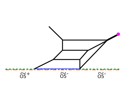
Figure 10: Another 5-brane web with an $\widetilde{\text{O5}}$-plane which gives the pure $G_{2}$ gauge theory. The diagram can be obtained by applying the same Higgsing procedure in Figure 9 to the diagram in Figure 4.

The diagram in Figure 10 is obtained by moving one of the half D7-brane which was sent to the infinitely left to the infinitely right. Then the D5-brane on the O5-plane disappears and we have an $\widetilde{\text{O5}}$-plane realized with the half monodromy cut.

2.3 Check from effective prepotential

In this subsection, we see evidence that the 5-brane web diagram in Figure 10 yields the 5d pure $G_{2}$ gauge theory from the analysis effective prepotentials.

In general, the effective prepotential of a 5d gauge theory with a gauge group $G$ is given by Seiberg:1996bd ; Morrison:1996xf ; Intriligator:1997pq

$$\mathcal{F}(\phi)=\frac{1}{2}m_{0}h_{ij}\phi_{i}\phi_{j}+\frac{\kappa}{6}d_{ijk}\phi_{i}\phi_{j}\phi_{k}+\frac{1}{12}\left(\sum_{r\in\text{roots}}\left|r\cdot\phi\right|^{3}-\sum_{f}\sum_{w\in{\bf R}_{f}}\left|w\cdot\phi+m_{f}\right|^{3}\right),$$ (1)

where $m_{0}$ is the inverse of the squared gauge coupling, $\phi_{i}$ are the Coulomb branch moduli, $\kappa$ is the classical Chern-Simons level and $m_{f}$ is the mass of a hypermultiplet in the representation ${\bf R}_{f}$ of $G$. $r$ are the roots of $G$ and $w$ are the weights of the representation ${\bf R}_{f}$. We also used $h_{ij}=\text{Tr}(T_{i}T_{j})$ and $d_{ijk}=\frac{1}{2}\text{Tr}\left(T_{i}\{T_{j},T_{k}\}\right)$ where $T_{i}$ are the Cartan generators of $G$.

In the following, we consider the prepotential of the pure $SO(7)$ gauge theory, the $SO(7)$ gauge theory with a spinor and then the pure $G_{2}$ gauge theory step by step.

Pure $SO(7)$.

The first example is the 5d pure $SO(7)$ gauge theory. When we parameterize the Coulomb branch moduli $\phi_{i}$ in the Dynkin basis, the prepotential of the pure $SO(7)$ gauge theory becomes

$$\mathcal{F}_{SO(7)}(\phi)= m_{0}(\phi_{1}^{2}-\phi_{1}\phi_{2}+\phi_{2}^{2}-2\phi_{2}\phi_{3}+2\phi_{3}^{2})$$ (2)

$$+\frac{4}{3}\phi_{1}^{3}-\frac{1}{2}\phi_{1}^{2}\phi_{2}-\frac{1}{2}\phi_{1}\phi_{2}^{2}+\frac{4}{3}\phi_{2}^{3}-3\phi_{2}^{2}\phi_{3}+2\phi_{2}\phi_{3}^{2}+\frac{4}{3}\phi_{3}^{3},$$ (3)

where we chose $[2,-1,0],[-1,2,-2],[0,-1,2]$ for the simple roots for defining the Weyl chamber. The tension of a monopole string may be computed by taking a derivative with respect to a Coulomb branch modulus. The monopole string tension from the prepotential (3) is

$$\frac{\partial\mathcal{F}_{SO(7)}}{\partial\phi_{1}}= \frac{1}{2}(2\phi_{1}-\phi_{2})(2m_{0}+4\phi_{1}+\phi_{2}),$$ (4)

$$\frac{\partial\mathcal{F}_{SO(7)}}{\partial\phi_{2}}= \frac{1}{2}(-\phi_{1}+2\phi_{2}-2\phi_{3})(2m_{0}+\phi_{1}+4\phi_{2}-2\phi_{3}),$$ (5)

$$\frac{\partial\mathcal{F}_{SO(7)}}{\partial\phi_{3}}= (-\phi_{2}+2\phi_{3})(2m_{0}+3\phi_{2}+2\phi_{3}).$$ (6)

It is also possible to compute the tension of a monopole string from 5-brane web diagrams. Monopole strings in a 5d gauge theory are realized by D3-branes which stretch along some face bounded by 5-branes. Therefore, the tension of a monopole string corresponds to the area of a face where a D3-brane can extend. Hence we need to compute the area of faces in the diagram in Figure 2 for the pure $SO(7)$ gauge theory.

For that, we first need to identify the gauge theory parameters with the length of 5-branes in the diagram in Figure 2. The height of the color D5-branes is the Coulomb branch modulus and we denote the height of the bottom color D5-brane, the middle color D5-brane and the top color D5-brane by $a_{1},a_{2},a_{3}$ respectively. In order to compute the inverse of the squared gauge coupling, we first turn off all the Coulomb branch moduli. Then the external $(2,1)$ 5-brane and the external $(1,-1)$ directly intersect with the O5-plane and the length of the D5-branes between the $(2,1)$ 5-brane and the $(1,-1)$ 5-brane on the O5-plane gives $m_{0}$. Alternatively, one can extrapolate the external $(2,1)$ 5-brane and the external $(1,-1)$ 5-brane in Figure 2 to the position of the O5-plane and measure the distance between the external $(2,1)$ 5-brane and the external $(1,-1)$ 5-brane on the O5-plane. The gauge theory parameterization for the pure $SO(7)$ gauge theory is summarized in Figure 11.

Figure 11: A gauge theory parameterization for the pure $SO(7)$ gauge theory. $a_{1},a_{2},a_{3}$ are the Coulomb branch moduli and $m_{0}$ is the inverse of the squared gauge coupling.

By using the parameterization depicted in Figure 11, we compute the area of faces in the pure $SO(7)$ diagram in Figure 2. We label the faces as in Figure 12.

Figure 12: Labeling for the three faces in the pure $SO(7)$ diagram.

The area of the three faces becomes

$$\scriptsize1⃝= \frac{1}{2}(a_{3}-a_{2})(2m_{0}+a_{2}+5a_{3}),$$ (7)

$$\scriptsize2⃝= \frac{1}{2}(a_{2}-a_{1})(2m_{0}-a_{1}+3a_{2}+4a_{3}),$$ (8)

$$\scriptsize3⃝= \frac{1}{2}a_{1}(2m_{0}+a_{1}+4a_{2}+4a_{3}).$$ (9)

We can then compare the are (7), (8) and (9) with the tension (4), (5) and (6). In the computation of the area from the pure $SO(7)$ diagram we parameterized the Coulomb branch moduli $a_{1},a_{2},a_{3}$ in the orthonormal basis of $\mathbb{R}^{3}$. The relation between $a_{1},a_{2},a_{3}$ and $\phi_{1},\phi_{2},\phi_{3}$ is

$$\phi_{1}=a_{3},\quad\phi_{2}=a_{2}+a_{3},\quad\phi_{3}=\frac{1}{2}(a_{1}+a_{2}+a_{3}).$$ (10)

Then the comparison of (7), (8) and (9) with (4), (5) and (6) yields

$$\scriptsize1⃝= \frac{\partial\mathcal{F}_{SO(7)}}{\partial\phi_{1}},$$ (11)

$$\scriptsize2⃝= \frac{\partial\mathcal{F}_{SO(7)}}{\partial\phi_{2}},$$ (12)

$$2\times\scriptsize3⃝= \frac{\partial\mathcal{F}_{SO(7)}}{\partial\phi_{3}}.$$ (13)

Therefore, a D3-brane can stretch along the region $\scriptsize1⃝$ or the region $\scriptsize2⃝$. On the other hand, one needs to double the area of the region $\scriptsize3⃝$, which implies that a D3-brane will not end on the $\widetilde{\text{O5}}^{-}$-plane and will end on a mirror D5-brane.

$SO(7)$ with a massless spinor.

The next example is the $SO(7)$ gauge theory with a hypermultiplet in the spinor representation. For simplicity we consider a case where the spinor matter is massless. In this case, there are several phases where the effective mass of the hypermultiplets vanishes. We here choose a phase where $[0,0,1],[0,1,-1],[1,-1,1],[-1,0,1]$ among the weights of the spinor representation are positive. Then the prepotential of the $SO(7)$ gauge theory with a massless spinor becomes

$$\mathcal{F}_{SO(7)_{s}}= m_{0}(\phi_{1}^{2}-\phi_{1}\phi_{2}+\phi_{2}^{2}-2\phi_{2}\phi_{3}+2\phi_{3}^{2})$$ (14)

$$+\frac{4}{3}\phi_{1}^{3}-\phi_{1}\phi_{2}^{2}+\frac{4}{3}\phi_{2}^{3}-\phi_{1}^{2}\phi_{3}+\phi_{1}\phi_{2}\phi_{3}-3\phi_{2}^{2}\phi_{3}+2\phi_{2}\phi_{3}^{2}+\phi_{3}^{3}.$$ (15)

The monopole string tension is then

$$\frac{\partial\mathcal{F}_{SO(7)_{s}}}{\partial\phi_{1}}= (2\phi_{1}-\phi_{2})(m_{0}+2\phi_{1}+\phi_{2}-\phi_{3}),$$ (16)

$$\frac{\partial\mathcal{F}_{SO(7)_{s}}}{\partial\phi_{2}}= (-\phi_{1}+2\phi_{2}-2\phi_{3})(m_{0}+2\phi_{2}-\phi_{3}),$$ (17)

$$\frac{\partial\mathcal{F}_{SO(7)_{s}}}{\partial\phi_{3}}= m_{0}(-2\phi_{2}+4\phi_{3})-\phi_{1}^{2}+\phi_{1}\phi_{2}-3\phi_{2}^{2}+4\phi_{2}\phi_{3}+3\phi_{3}^{2}.$$ (18)

Let us then compute the area of faces in a diagram for the $SO(7)$ gauge theory with a massless spinor. We need to use a particular diagram which corresponds to the phase we chose to compute the prepotential (15). Such a diagram is depicted in Figure 13 and we label the four faces in the diagram.

Figure 13: A 5-brane web diagram of the $SO(7)$ gauge theory with a massless spinor. The mass is related to the length between the parallel $(2,1)$ 5-branes and they are on top of each other in the massless limit. We also label the four faces in the diagram.

The Coulomb branch moduli $a_{1},a_{2},a_{3}$ are again the height of the bottom color D5-brane, the middle color D5-brane and the top color D5-brane respectively. We also extrapolate the external $(2,1)$ 5-brane and the external $(1,-1)$ 5-brane on top of the $\widetilde{\text{O5}}$-plane and the distance between the extrapolated external 5-branes is the inverse of the squared gauge coupling $m_{0}$. The gauge theory parameterization is summarized in Figure 14.

Figure 14: A gauge theory parameterization for the $SO(7)$ gauge theory with a massless spinor. $a_{1},a_{2},a_{3}$ are the Coulomb branch moduli and $m_{0}$ is the inverse of the squared gauge coupling.

We can now compute the area of the four faces in Figure 13 by the parameterization in Figure 14. The result is

$$\scriptsize1⃝= \frac{1}{2}(a_{3}-a_{2})(2m_{0}-a_{1}+a_{2}+5a_{3}),$$ (19)

$$\scriptsize2⃝= \frac{1}{2}(a_{2}-a_{1})(2m_{0}-a_{1}+3a_{2}+3a_{3}),$$ (20)

$$\scriptsize3⃝= \frac{1}{2}a_{1}(2m_{0}+a_{1}+3a_{2}+3a_{3}),$$ (21)

$$\scriptsize4⃝= \frac{1}{4}(-a_{1}^{2}+2a_{1}a_{2}-a_{2}^{2}+2a_{1}a_{3}+2a_{2}a_{3}-a_{3}^{2}).$$ (22)

The comparision of (19), (20), (21) and (22) with (16), (17) and (18) yields relations

$$\scriptsize1⃝= \frac{\partial\mathcal{F}_{SO(7)_{s}}}{\partial\phi_{1}},$$ (23)

$$\scriptsize2⃝= \frac{\partial\mathcal{F}_{SO(7)_{s}}}{\partial\phi_{2}},$$ (24)

$$2\times\scriptsize3⃝+\scriptsize4⃝= \frac{\partial\mathcal{F}_{SO(7)_{s}}}{\partial\phi_{3}},$$ (25)

using the relation (10). As in the case of the pure $SO(7)$ gauge theory, we need to double the area of the region $\scriptsize3⃝$. In fact, we further need to add the area of the region $\scriptsize4⃝$ for the monopole string tension corresponding to $\frac{\partial\mathcal{F}_{SO(7)_{s}}}{\partial\phi_{3}}$. This fact becomes important also for the comparison of the monopole tension in the case of the pure $G_{2}$ gauge theory.

Pure $G_{2}$.

Finally we consider the prepotential of the pure $G_{2}$ gauge theory. When we use the Dynkin basis for parametrizing the Coulomb branch moduli $\phi_{i}$, the prepotential of the 5d pure $G_{2}$ gauge theory becomes

$$\mathcal{F}_{G_{2}}(\phi)=m_{0}(\phi_{1}^{2}-3\phi_{1}\phi_{2}+3\phi_{2}^{2})+\frac{4}{3}\phi_{1}^{3}-4\phi_{1}^{2}\phi_{2}+3\phi_{1}\phi_{2}^{2}+\frac{4}{3}\phi_{2}^{3},$$ (26)

where we chose $[2,-3]$ and $[-1,2]$ for the simple roots for defining the Weyl chamber. Hence the expected monopole tension from the prepotential (26) is

$$\frac{\partial\mathcal{F}_{G_{2}}}{\partial\phi_{1}} = (m_{0}+2\phi_{1}-\phi_{2})(2\phi_{1}-3\phi_{2}),$$ (27)

$$\frac{\partial\mathcal{F}_{G_{2}}}{\partial\phi_{2}} = (-\phi_{1}+2\phi_{2})(3m_{0}+4\phi_{1}+2\phi_{2}).$$ (28)

The gauge theory parameterization for the pure $G_{2}$ gauge theory realized in Figure 10 can be understood in a similar way to the case of the $SO(7)$ gauge theories. We denote the height of the lowest color D5-brane by $a_{1}$ and the height of the second lowest color D5-brane by $a_{2}$ as in Figure 15.

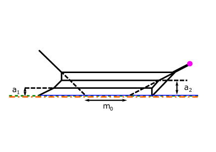
Figure 15: A gauge theory parameterization for the pure $G_{2}$ gauge theory. $a_{1},a_{2}$ are the Coulomb branch moduli and $m_{0}$ is related to the inverse of the gauge coupling.

The inverse of the square gauge coupling can be calculated from the distance between the extrapolated external $(2,1)$ 5-brane and the external $(1,-1)$ 5-brane and it is denoted by $m_{0}$ in Figure 15. We are now able to compute the area corresponding to the tension of monopoles strings by using the parameters in Figure 15. We label four faces in the pure $G_{2}$ diagram as in Figure 16.

Figure 16: Labeling for the four faces in the pure $G_{2}$ diagram. Note that the regions $\scriptsize1⃝$ and $\scriptsize4⃝$ are not separated by a 5-brane and are connected to each other.

The area of the four regions is

$$\scriptsize1⃝ = a_{1}(m_{0}+2a_{1}+3a_{2}),$$ (29)

$$\scriptsize2⃝ = (a_{2}-a_{1})(m_{0}+a_{1}+3a_{2}),$$ (30)

$$\scriptsize3⃝ = a_{1}(m_{0}+2a_{1}+3a_{2}),$$ (31)

$$\scriptsize4⃝ = a_{1}a_{2}.$$ (32)

We can deduce which area we should compare with the monopole string tension (27) and (28) from the analysis of the $SO(7)$ gauge theory with a massless spinor. For the $SO(7)$ gauge theory with a spinor, the area corresponding to the monopole string tension is $\scriptsize1⃝$, $\scriptsize2⃝$, $2\times\scriptsize3⃝+\scriptsize4⃝$. After the Higgsing, the region $\scriptsize1⃝$ is combined with $\scriptsize4⃝$, hence the area corresponding to the monopole string tension for the pure $G_{2}$ gauge theory should be $\scriptsize2⃝$ and $\scriptsize1⃝+2\times\scriptsize3⃝+\scriptsize4⃝$. Such an area is given by

$$\scriptsize2⃝ = (a_{2}-a_{1})(m_{0}+a_{1}+3a_{2}),$$ (33)

$$\scriptsize1⃝+2\times\scriptsize3⃝+\scriptsize4⃝ = a_{1}(3m_{0}+6a_{1}+10a_{2}).$$ (34)

We compare the tension (27) and (28) computed from the prepotential (26) with the tension (33) and (34) from the area of the 5-brane web in Figure 16. Note that the Coulomb branch moduli $a_{1},a_{2}$ are related to $\phi_{1},\phi_{2}$ by

$$2\phi_{1}-3\phi_{2}=a_{2}-a_{1},\quad-\phi_{1}+2\phi_{2}=a_{1}.$$ (35)

Using the relation (35), we can see that

$$\scriptsize2⃝= \frac{\partial\mathcal{F}_{G_{2}}}{\partial\phi_{1}},$$ (36)

$$\scriptsize1⃝+2\times\scriptsize3⃝+\scriptsize4⃝= \frac{\partial\mathcal{F}_{G_{2}}}{\partial\phi_{2}}.$$ (37)

We note that the Higgsing of the $SO(7)$ gauge theory with a spinor enforces the parameters for the $SO(7)$ gauge theory to be $a_{3}=a_{1}+a_{2}$ in Figure 14. This means that the $SO(7)$ Coulomb branch moduli satisfy $\phi_{1}=\phi_{3}$. With the proper map between the $SO(7)$ Coulomb branch moduli $\phi_{i}^{SO(7)}$ and the $G_{2}$ Coulomb moduli $\phi^{G_{2}}_{j}$ given by $\phi_{1}^{SO(7)}\to\phi^{G_{2}}_{2}$ and $\phi_{2}^{SO(7)}\to\phi_{1}^{G_{2}}$, one can easily see that the prepotential for 5d $SO(7)$ gauge theory with a spinor (15) becomes the $G_{2}$ prepotential (26). It follows that the tensions of the monopole strings are also consistent with the Higgsing

$$\frac{\partial\mathcal{F}_{SO(7)_{s}}}{\partial\phi_{2}}{}\Big{|}_{\rm Higgsing} =~{}\frac{\partial\mathcal{F}_{G_{2}}}{\partial\phi_{1}},\qquad\Big{(}\frac{\partial\mathcal{F}_{SO(7)_{s}}}{\partial\phi_{1}}+\frac{\partial\mathcal{F}_{SO(7)_{s}}}{\partial\phi_{3}}\Big{)}{}\Big{|}_{\rm Higgsing}=\frac{\partial\mathcal{F}_{G_{2}}}{\partial\phi_{2}},$$ (38)

or in other words, through the Higgsing, (18) $\to$ (36) and agrees with (16) $+$(18), $\to$ (37). The analysis of the prepotential therefore presents further support for the claim that the diagram in Figure 10 realizes the 5d pure $G_{2}$ gauge theory.

2.4 Adding flavors to $G_{2}$

5d $G_{2}$ gauge theories may have hypermultiplets in the fundamental representation and the maximal number flavors for a $G_{2}$ gauge theory to have a 5d UV fixed point is five Zafrir:2015uaa ; Jefferson:2017ahm . From the viewpoint of 5-brane webs, one can also add hypermultiplets in the fundamental representation of $G_{2}$ to the 5-brane web diagram in Figure 10. There are two ways to introduce flavors for the $G_{2}$ theory. One way uses the vector matter of the $SO(7)$ gauge theory and the other way utilizes the spinor matter of the $SO(7)$ gauge theory. After the Higgsing from $SO(7)$ to $G_{2}$, the former becomes the fundamental matter of the $G_{2}$ gauge theory and the latter becomes the fundamental matter plus a singlet hypermultiplet of the $G_{2}$ gauge theory. The singlet appears since the spinor representation of $SO(7)$ is the eight-dimensional representation and the fundamental representation of $G_{2}$ is the seven-dimensional representation. Hence, the Higgsing of the $SO(7)$ gauge theory with a hypermultiplet in the vector representation and a hypermultiplet in the spinor representation gives the $G_{2}$ gauge theory with one flavor, and similarly the Higgsing of the $SO(7)$ gauge theory with two hypermultiplets in the spinor representation gives the $G_{2}$ gauge theory with one flavor and a singlet. The two 5-brane diagrams giving the $G_{2}$ gauge theories with one flavor are depicted in Figure 17 and 17.

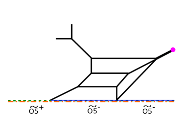
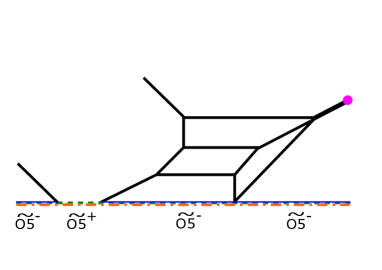
Figure 17: 5-brane web diagrams of the $G_{2}$ gauge theory with one flavor. (a): The diagram is obtained by Higgsing the $SO(7)$ gauge theory with one vector and one spinor. The resulting theory is $G_{2}$ gauge theory with one flavor. (b): The diagram is obtained by Higgsing the $SO(7)$ gauge theory with two spinors. The resulting theory is the $G_{2}$ gauge theory with one flavor and a singlet.

It is straightforward to add more flavors to $G_{2}$ gauge theories by Higgsing the 5d $SO(7)$ gauge theory with one spinor and more than one hypermultiplets either in the vector representation or the spinor representation. An example of a 5-brane web diagram for the $G_{2}$ gauge theory with two flavors is depicted in Figure 18.

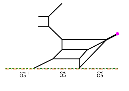
Figure 18: A 5-brane diagram for the $G_{2}$ gauge theory with two flavors.

As for the 5-brane web obtained by Higgsing the $SO(7)$ gauge theories with two spinors, one can also perform the generalized flop transition in Figure 8 and then the 5-brane diagram becomes the one in Figure 19. It is also possible to obtain an equivalent diagram by moving the half D7-brane associated the monodromy cut from the infinitely right to the infinitely left in Figure 19, and the resulting diagram after the transition is given in Figure 19 without any branch cut.

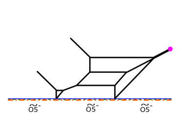
Figure 19: 5-brane diagrams for the $G_{2}$ gauge theory with one flavor and a singlet after performing the generalized flop transitions. (a): A 5-brane web for a $G_{2}$ gauge theory with one flavor which is obtained after performing the generalized flop transition to the diagram in Figure 17. The diagram contains only an $\widetilde{\text{O5}}^{-}$-plane. (b): An equivalent 5-brane web diagram to the one in Figure 19. We move the half D7-brane in the infinitely right to the infinitely left. Then the $\widetilde{\text{O5}}$-plane disappears and we only have an O5-plane. The diagram still yields the $G_{2}$ gauge theory with one flavor and a singlet.

3 Another 5-brane web for pure $G_{2}$ gauge theory

In this section, we present another 5-brane web diagram for the 5d pure $G_{2}$ gauge theory without using an $\widetilde{\text{O5}}$-plane different to the one in section 2. This diagram turns out to be useful for the topological vertex computation in section 4.

3.1 Higgsing 5d $SO(8)$ gauge theory with one spinor and one conjugate spinor

In section 2, we used the 5-brane web diagram in Figure 5 for the 5d $SO(7)$ gauge theory with one spinor and the Higgsing of the diagram yielded the web diagram for the pure $G_{2}$ gauge theory in Figure 9. The 5-brane diagram of the 5d $SO(7)$ gauge theory has been originally obtained by the Higgsing associated to vector matter of the 5d $SO(8)$ gauge theory. In other words, the 5-brane web diagram of the pure $G_{2}$ gauge theory in Figure 9 was obtained by the two successive Higgsings from the 5d $SO(8)$ gauge theory with one vector and one spinor. Due to the triality of the 5d $SO(8)$ gauge theory, the 5d $SO(8)$ gauge theory with one vector and one spinor is equivalent to the 5d $SO(8)$ gauge theory with one spinor and one conjugate spinor. Therefore, we should again obtain a 5-brane web diagram for the pure $G_{2}$ gauge theory by Higgsing a 5-brane web for the 5d $SO(8)$ gauge theory with one spinor and one conjugate spinor.

To introduce a hypermultiplet in the spinor representation to the 5-brane web diagram for the 5d $SO(8)$ gauge theory, we consider a “quiver theory” of $SO(8)-USp(0)$ and the $USp(0)$ instanton plays a role of the spinor matter Zafrir:2015ftn . For introducing two spinors, we consider a quiver $USp(0)-SO(8)-USp(0)$. However, we need two spinors of opposite chirality. The difference between a spinor and a conjugate spinor can be realized by considering different discrete theta angles for the two $USp(0)$ gauge groups Zafrir:2015ftn . Namely, we consider a 5-brane diagram of the quiver $USp(0)-SO(8)-USp(0)$ but the two $USp(0)$ gauge groups have different discrete theta angles.

A 5-brane web diagram of the 5d $SO(8)$ gauge theory with one spinor and one conjugate spinor is given in Figure 20.

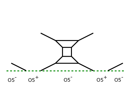
Figure 20: A 5-brane web diagram for the 5d $SO(8)$ gauge theory with one spinor and one conjugate spinor. The discrete theta angle of the two $USp(0)$ theories is different from each other although the difference is not explicitly expressed in the diagram.

Note that there are two parallel external $(2,1)$ 5-branes and two parallel external $(2,-1)$ 5-branes. Each two parallel external 5-branes implies an $SU(2)$ flavor symmetry and hence the theory shows an $SU(2)\times SU(2)$ perturbative flavor symmetry from one spinor and one conjugate spinor. At the level of the diagram in Figure 20, the difference of the discrete theta angle is invisible. However, the difference appears after the generalized flop transition Hayashi:2017btw . The two different types of the flop transitions depending on the discrete theta angle are depicted in Figure 21.

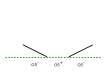
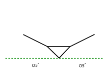
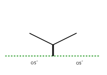
Figure 21: The generalized flop transition for the 5-brane web for $USp(0)$. Depending on the discrete theta angle, the transition changes the figure (a) into either figure (b) or figure (c).

We can then apply the generalized flop transition in Figure 21 to the diagram in Figure 20 and it yields another 5-brane web diagram for the 5d $SO(8)$ gauge theory with one spinor and one conjugate spinor. The resulting diagram is depicted in Figure 22.

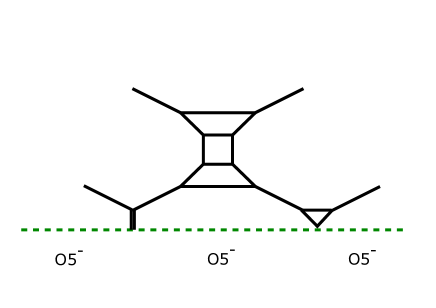
Figure 22: A 5-brane web diagram for the 5d $SO(8)$ gauge theory with one spinor and one conjugate spinor after performing the generalized flop transitions.

In order to perform the Higgsing to the 5d pure $G_{2}$ gauge theory, we consider a further transition given in Figure 6, yielding a 5-brane web in Figure 23.

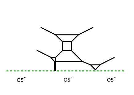
Figure 23: Another 5-brane web diagram for the 5d $SO(8)$ gauge theory with one spinor and one conjugate spinor.

We can use the 5-brane web in Figure 23 to obtain another 5-brane web diagram for the 5d pure $G_{2}$ gauge theory by two Higgsings. Let us first perform a Higgsing associated to the parallel external $(2,1)$ 5-branes on the right part in Figure 23. The procedure is essentially the same as what has been done in Figure 9 and the resulting 5-brane web diagram is given in Figure 24.

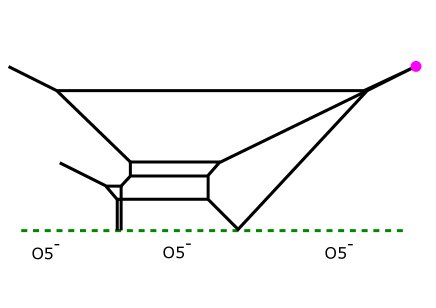
Figure 24: Another 5-brane web diagram for the 5d $SO(7)$ gauge theory with one spinor.

Due to the triality, the 5-brane web diagram in Figure 24 should give rise to the 5d $SO(7)$ gauge theory with one spinor. Hence the diagram in Figure 24 realizes the $SO(7)$ gauge group without introducing an $\widetilde{\text{O5}}$-plane different from the diagram in Figure 4.

Since the diagram in Figure 24 still contains parallel external $(2,-1)$ 5-branes, we can perform a Higgsing associated to them. Note that after the Higgsing, the consistency of the diagram restricts the position of the lowest color D5-brane to the location of the O5-plane. The resulting diagram is depicted in Figure 25.

Figure 25: Another 5-brane web diagram for the 5d pure $G_{2}$ gauge theory.

The 5-brane web diagram of the pure $G_{2}$ gauge theory is given without an $\widetilde{\text{O5}}$-plane in this case. In fact, it turns out that this diagram is more useful to apply the topological vertex technique to compute the partition function than the diagram in Figure 10.

3.2 Check from effective prepotential

As we have done in section 2.3, we can give evidence that the diagram in Figure 25 yields the pure $G_{2}$ gauge theory by computing the tension of a monopole string from the diagram. For that, we first associate the gauge theory parameters, the Coulomb branch moduli $a_{1},a_{2}$ and the inverse of the squared gauge coupling $m_{0}$ to some lengths of 5-branes. $a_{1}$ is the height of the lowest color D5-brane and $a_{2}$ is the height of the second lowest D5-brane. $m_{0}$ is determined by extrapolating the external $(2,1)$ 5-brane and the external $(2,-1)$ 5-brane to the location of the O5-plane. The relations between the gauge theory parameters and the lengths of 5-branes are depicted in Figure 26.

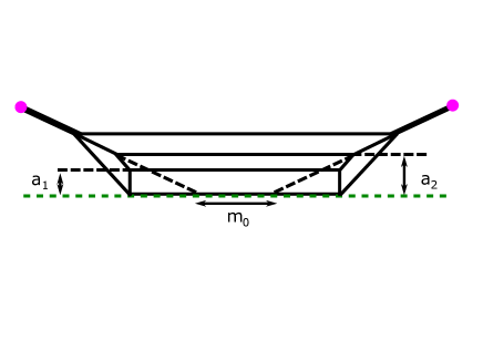
Figure 26: A gauge theory parameterization for the pure $G_{2}$ gauge theory for the diagram in Figure 25. $a_{1},a_{2}$ are the Coulomb branch moduli and $m_{0}$ is related to the inverse of the squared gauge coupling.

The tension of a monopole string is given by the area of a face where a D3-brane stretch. There are five faces in the 5-brane web in Figure 25 and we denote the five faces by $\scriptsize1⃝$ - $\scriptsize5⃝$ as in Figure 27.

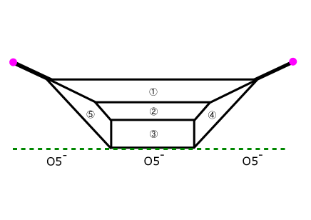
Figure 27: Labeling for the five faces in the pure $G_{2}$ diagram. Note that the regions $\scriptsize1⃝$, $\scriptsize4⃝$ and $\scriptsize5⃝$ are not separated by a 5-brane and are connected to each other.

The areas of the five faces are respectively

$$\scriptsize1⃝ = a_{1}(m_{0}+2a_{1}+4a_{2}),$$ (39)

$$\scriptsize2⃝ = (a_{2}-a_{1})(m_{0}+a_{1}+3a_{2}),$$ (40)

$$\scriptsize3⃝ = a_{1}(m_{0}+2a_{1}+2a_{2}),$$ (41)

$$\scriptsize4⃝ = a_{1}a_{2},$$ (42)

$$\scriptsize5⃝ = a_{1}a_{2}.$$ (43)

One face where a D3-brane stretch is $\scriptsize2⃝$. As for the other case, note that we needed to double the area of the region $\scriptsize3⃝$ and further add the area $\scriptsize4⃝$ as in Figure 16. Two sequences of Higgsing connect the region $\scriptsize1⃝$, $\scriptsize4⃝$ and $\scriptsize5⃝$. Hence, in this case the other face should be $\scriptsize1⃝+2\times\scriptsize3⃝+\scriptsize4⃝+\scriptsize5⃝$. Then, the area of the faces corresponding to the monopole string tension is

$$\scriptsize2⃝ = (a_{2}-a_{1})(m_{0}+a_{1}+3a_{2}),$$ (44)

$$\scriptsize1⃝+2\times\scriptsize3⃝+\scriptsize4⃝+\scriptsize5⃝ = a_{1}(3m_{0}+6a_{1}+10a_{2}),$$ (45)

which exactly reproduce the area (33) and (34) calculated from the diagram in Figure 10. Therefore the monopole tension computation gives another evidence that the diagram in Figure 25 yields the 5d pure $G_{2}$ gauge theory.

4 5d Nekrasov partition functions of $G_{2}$ gauge theories

In section 2 and section 3, we have constructed 5-brane web diagrams which realize 5d $G_{2}$ gauge theories. In section 2 we presented 5-brane webs for $G_{2}$ gauge theories using an $\widetilde{\text{O5}}$-plane and in section 3 we presented the 5-brane web for the pure $G_{2}$ gauge theory with an O5-plane. One of the applications of these 5-brane webs is to compute the BPS partition functions of 5d theories realized by the webs. Since 5-brane webs can be reinterpreted as toric diagrams Leung:1997tw , we can apply the topological vertex formalism Aganagic:2003db ; Iqbal:2007ii ; Awata:2008ed . In Kim:2017jqn , the topological vertex formalism for webs with an O5-plane has been developed and hence we can utilize the technique to compute the partition function for the pure $G_{2}$ gauge theory realized by the 5-brane web with an O5-plane. Although the 5-brane web diagrams in section 2 are realized with an $\widetilde{\text{O5}}$-plane, we extend the formalism so that it can apply to webs with an $\widetilde{\text{O5}}$-plane in section 4.1. Then we apply the method to compute the partition functions of the 5d pure $G_{2}$ gauge theory and the 5d $G_{2}$ gauge theory with one flavor.

4.1 Vertex formalism with an O5- and $\widetilde{\text{O5}}$-plane

Here, we first briefly review the topological vertex formalism for 5-brane webs with an O5-plane proposed in Kim:2017jqn . As for the 5-branes which do not touch the O5-plane, the rule is exactly the same as the conventional topological vertex formalism Aganagic:2003db : We first assign different Young diagrams $Y_{i}$ to different $(p,q)$ 5-branes. Then, we introduce the edge factor $(-Q)^{|Y|}f_{Y}{}^{n}$ to each edge, where $Q$ is given by the exponential of the length of the corresponding $(p,q)$ 5-brane. Here, $f_{Y}$ is the framing factor defined as

$$f_{Y}=(-1)^{|Y|}g^{\frac{1}{2}(||Y^{t}||^{2}-||Y||^{2})},$$ (46)

with $|Y|=\sum_{i}Y_{i}$ and $||Y||^{2}=\sum_{i}Y_{i}{}^{2}$. $n$ is a certain integer which is associated to the relative difference of the framing when we glue two topological vertices. The parameter $g$ is related to the Omega deformation parameters by $g=e^{-\epsilon_{1}}=e^{+\epsilon_{2}}$. We also introduce the topological vertex $C_{Y_{1}Y_{2}Y_{3}}$ to each vertex of a diagram, where the Young diagrams $Y_{1},Y_{2},Y_{3}$ are ordered clockwise. On top of that, the additional rule is given for $(p,-1)$ and $(-p,-1)$ 5-branes which intersect with each other on the O5-plane as depicted in Figure 28 (a). The point is to assign the identical Young diagram to these two 5-branes and to assign an edge factor

$$(+Q_{1}Q_{2})^{|Y|}f_{Y}{}^{\mathfrak{n}},\qquad(\mathfrak{n}=p_{1}q_{2}+p_{2}q_{1}+1),$$ (47)

corresponding to this part, where $Q_{1}$ and $Q_{2}$ are the exponential of the (rescaled) length of the two 5-branes respectively. By multiplying all these factors and by summing over all the possible Young diagrams, we obtain the topological string partition function.

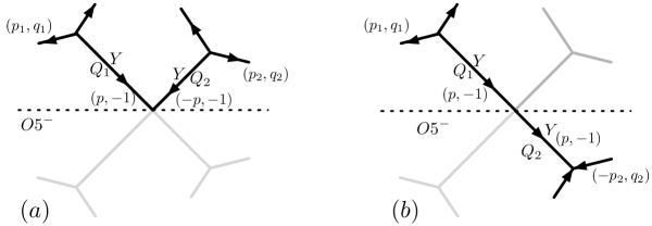
Figure 28: (a): The $(p,-1)$ and $(-p,-1)$ 5-branes which intersect with each other on the O5-plane. (b): An equivalent diagram to (a) but we use the mirror image for a part of the diagram.

Although we can compute the topological string partition function directly using the rules above with a configuration in Figure 28 (a), it turns out to be more convenient to cut the D5-branes with a finite length and to use the mirror image for a part of the diagram so that the two 5-branes which originally intersected with each other on the O5-plane become a single edge as in Figure 28 (b) Kim:2017jqn . This operation corresponds to using the identity

$$C_{Y_{1}Y_{2}Y_{3}}=(-1)^{|Y_{1}|+|Y_{2}|+|Y_{3}|}f_{Y_{1}}^{-1}f_{Y_{2}}^{-1}f_{Y_{3}}^{-1}C_{Y_{3}^{t}Y_{2}^{t}Y_{1}^{t}}.$$ (48)

to all the vertices reflected along the O5-plane because a clockwise direction is mapped to a counter-clockwise direction under this reflection. Note that the Young diagrams assigned to the edges reflected along the O5-plane should be transposed. After the proper reflection, each sub-diagram can be seen as a strip diagram. Such sub-amplitudes are already computed in Iqbal:2004ne . The strip amplitudes are written in terms of the product of the factor defined as

$$Z_{\nu}(g)=\prod_{(i,j)\in\nu}(1-g^{\nu_{i}+\nu_{j}^{t}-i-j+1}),$$ (49)

and the factor defined as

$$\mathcal{R}_{XY}(Q)=\mathcal{M}(Q)^{-1}\,\mathcal{N}_{X^{t}Y}(Q),$$ (50)

with

$$\mathcal{M}(Q)={\rm PE}\left[\frac{g}{(1-g)^{2}}Q\right],$$ (51)

where $\rm PE$ is the Plethystic exponential defined as

$${\rm PE}[f(\cdot)]=\exp\bigg{[}\sum_{i=1}^{\infty}\frac{1}{n}f(\cdot^{n})\bigg{]},$$ (52)

and

$$\mathcal{N}_{\lambda\mu}(Q)=\prod_{(i,j)\in\lambda}(1-Qg^{\lambda_{i}+\mu_{j}^{t}-i-j+1})\prod_{(i,j)\in\mu}(1-Qg^{-\lambda_{j}^{t}-\mu_{i}+i+j-1}).$$ (53)

What remains is to glue each strip at the edges where we cut before the reflection by multiplying corresponding edge factors and by summing over Young diagram assigned to these edges. In this process, we also need to take into account the additional factors of the form $(-1)^{|Y|}f_{Y}^{-1}$ in (48). If two vertices connected to the same edge are both reflected along the O5-plane, such contribution cancels with each other as $(-1)^{|Y|}f_{Y}^{-1}\times(-1)^{|Y^{t}|}f_{Y^{t}}^{-1}=1$. Only when one vertex is reflected while the other vertex is not, we need to multiply such a factor .

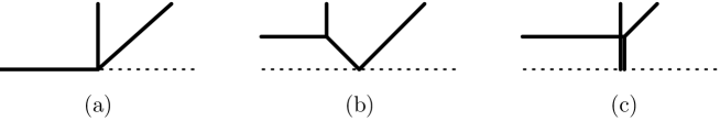
Figure 29: Configurations with an O5-plane

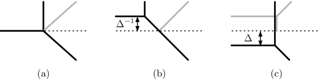
Figure 30: Configurations with an O5-plane with mirror image.

This method can be generalized to webs with an $\widetilde{\text{O5}}$-plane. As we did in section 2.1, we can interpret that an $\widetilde{\text{O5}}$-plane is realized between two fractional D7-branes on top of the O5-plane placed at infinitely left and infinitely right, respectively Zafrir:2015ftn ; Feng:2000eq . The point is to convert an $\widetilde{\text{O5}}$-plane to an O5-plane by moving one of these fractional D7-branes to the other side by using Hanany-Witten transition as discussed in Figure 5. After that, it can be seen as a special case of a 5-brane web with an O5-plane. For example, as is also mentioned in section 2, the diagram in Figure 29 (a) can be understood as a special case of the ones in Figure 29 (b) or (c). As discussed above, by considering the mirror image as in Figure 30 (b) or (c), we can interpret the configurations as a part of trip diagrams. Therefore, a configuration with Figure 29 (a) should be also considered as a special case of Figure 30 (b) or (c), where we tune the K$\ddot{\text{a}}$hler parameter $\Delta\to 1$ so that the position of the D5-brane comes to exactly the place where the O5-plane exists.

4.2 Pure $G_{2}$ gauge theory

We apply the technique of the topological vertex for webs involving an O5-plane or an $\widetilde{\text{O5}}$-plane described in section 4.1 to the 5-brane web of 5d $G_{2}$ gauge theories. We first consider a 5-brane web for the 5d pure $G_{2}$ gauge theory. So far we have presented two types of the 5-brane webs for the pure $G_{2}$ gauge theory. One is depicted in Figure 10 with an $\widetilde{\text{O5}}$-plane and the other is depicted in Figure 25 with an O5-plane. For applying the topological vertex formalism it is appropriate to use the one in Figure 25 since the diagram in Figure 10 has a configuration where a single 5-brane directly intersects with an O5-plane and we have not yet known the vertex rule for such a configuration.

We use the 5-brane diagram in Figure 25 to compute the partition function of the 5d pure $G_{2}$ gauge theory. First we introduce the gauge theory parameters for the diagram as in Figure 26. The Coulomb branch moduli $a_{1},a_{2}$ of the pure $G_{2}$ gauge theory are given by the height of the bottom and the second bottom color D5-brane respectively. We then define $A_{1},A_{2}$ by

$$A_{1}=e^{-a_{1}},\qquad A_{2}=e^{-a_{2}},\qquad$$ (54)

which are the parameters directly appearing in the partition function. For the convenience of the later computation, we also introduce

$$A_{0}=1,\qquad A_{-1}=A_{1}^{-1}A_{2}^{-1},$$ (55)

and define

$$Q_{ij}=A_{i}A_{j}{}^{-1},\qquad(-1\leq j<i\leq 2).$$ (56)

The inverse of the squared gauge coupling is given by $m_{0}$ in Figure 26 and we define the instanton fugacity by

$$q=e^{-m_{0}}.$$ (57)

Then the K$\ddot{\text{a}}$hler parameters associated to the length of the horizontal lines in Figure 31 are

$$Q_{B_{2}}=qA_{2}{}^{4},\qquad Q_{B_{1}}=Q_{B_{0}}=qA_{1}{}^{2}A_{2}{}^{2},\qquad Q_{B_{-1}}=qA_{1}{}^{4}A_{2}{}^{4}.$$ (58)

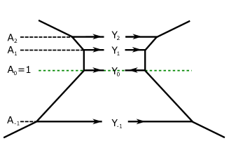
Figure 31: (a): The assignment of the Young diagrams $Y_{i},i=-1,0,1,2$ and the K$\ddot{\text{a}}$hler parameter $Q_{B_{i}},i=-1,0,1,2$ for the diagram in Figure 25 of the pure $G_{2}$ gauge theory. (b): An equivalent diagram to the one in Figure 31. We use the mirror image for the outmost 5-brane in Figure 31. As for the bottom 5-brane in Figure 31, we use the mirror image for the left part and use the original one for the right part.

With the parameterization, we compute the topological string partition function by applying the topological vertex to the 5-brane web in Figure 25. Since the diagram involves an O5-plane, we utilize the method in section 4.1. First, we cut the color D5-branes in Figure 31 in the middle and use the mirror image for the outmost 5-brane for describing the diagram as in Figure 31. The diagram now consists of two strip diagrams. Note that the diagram in Figure 31 is almost the same as the diagram of the pure $SU(4)$ gauge theory of CS level zero with $A_{0}$ set to $1$. A difference comes from the assignment of the Young diagram for $Y_{0}$. In order to see it, recall the diagram of the 5d $SO(7)$ gauge theory with one spinor in Figure 24, which is the diagram before Higgsing to the one in Figure 25. Let us cut then the diagram in Figure 24 in the middle into the left part and the right part and use the mirror image for a part of the diagram to apply the topological vertex computation in section 4.1. Then we use the mirror image for the bottom color D5-brane in the left part while we use the original bottom color D5-brane for the right part in the upper half plane. After the Higgsing, the bottom color D5-brane in Figure 24 becomes the color D5-brane on top of an O5^--plane in Figure 25. Therefore, when we consider the diagram in Figure 31, we should transpose the Young diagram $Y_{0}$ in the left strip while we keep the Young diagram $Y_{0}$ in the right strip. This is essentially the only difference from the 5-brane web of the pure $SU(4)$ gauge theory. The Young diagram assignment is summarized in Figure 31.

It is now straightforward to apply the topological vertex formalism to the diagram in Figure 31. It is useful to compute the partition function for the left strip and the right strip separately first and glue them together later. The partition function for the left strip is given by

$$Z^{\rm strip1}(\{Q_{ij}\};Y_{-1},Y_{0},Y_{1},Y_{2})=\prod_{i=-1}^{2}g^{\frac{1}{2}||Y_{i}||^{2}}\prod_{i=-1}^{2}Z_{Y_{i}}(g)\prod_{-1\leq j<i\leq 2}\mathcal{R}_{Y_{i}Y_{j}^{t}}(Q_{ij})^{-1}.$$ (59)

The partition function of the right strip can be expressed as $Z^{\rm strip2}(\{Q_{ij}\};Y_{-1},Y_{0}^{t},Y_{1},Y_{2})$ with

$$Z^{\rm strip2}(\{Q_{ij}\};Y_{-1},Y_{0},Y_{1},Y_{2})=\prod_{i=-1}^{2}g^{\frac{1}{2}||Y_{i}^{t}||^{2}}\prod_{i=-1}^{2}Z_{Y_{i}}(g)\prod_{-1\leq j<i\leq 2}\mathcal{R}_{Y_{i}Y_{j}^{t}}(Q_{ij})^{-1}.$$ (60)

The rest is gluing the contribution of the left strip and the right strip to each other. When we glue these two sub-diagram, we should also take into account the effect of flipping the Young diagram, which is given by the extra factor of the form $(-1)^{|Y_{0}|}f_{Y_{0}}$ coming from the identity (48). Note that such factor for the upper most D5-brane cancels out as discussed in section 4.1 since the whole edge is reflected. Then, the topological string partition function for the diagram in Figure 31 is

$$Z_{G_{2}}= \sum_{\{Y_{i}\}}(-1)^{|Y_{0}|}f_{Y_{2}}^{3}f_{Y_{1}}f_{Y_{0}}f_{Y_{-1}}^{-3}\prod_{i=-1}^{2}(-Q_{B_{i}}){}^{|Y_{i}|}$$ (61)

$$Z^{\rm strip1}(\{Q_{ij}\};Y_{-1},Y_{0},Y_{1},Y_{2})Z^{\rm strip2}(\{Q_{ij}\};Y_{-1},Y_{0}^{t},Y_{1},Y_{2}).$$ (62)

We claim that this is the partition function of the 5d pure $G_{2}$ gauge theory up to the perturbative contribution of the Cartan subalgebra of the pure $G_{2}$ which should be added by hand in the topological vertex computation. Notice that the only difference between this $G_{2}$ partition function and the pure $SU(4)$ partition function with $A_{0}=1$ in (55) is as follows: The Young diagram $Y_{0}$ in $Z^{\rm strip2}$ is transposed, the power of framing factor $f_{Y_{0}}$ is 1 instead of $-1$, and also the associated sign factor $(-)^{|Y_{0}|}$ is present.

Perturbative part.

Let us look at the partition function (61) in more detail. The perturbative part of the partition function is obtained by considering a limit $q\to 0$. The limit corresponds to the restriction of the Young diagrams $Y_{i}=\emptyset$ for $i=-1,0,1,2$. Then the partition function (61) is simplifies and is given by

$$Z_{\text{pert}}= \mathcal{M}(A_{1})^{2}\mathcal{M}(A_{1}^{-1}A_{2})^{2}\mathcal{M}(A_{2})^{2}\mathcal{M}(A_{1}A_{2})^{2}\mathcal{M}(A_{1}^{2}A_{2})^{2}\mathcal{M}(A_{1}A_{2}^{2})^{2}$$ (63)

$$= {\rm PE}\left(\frac{2g}{(1-g)^{2}}(A_{1}+A_{2}+A_{1}A_{2}+A_{1}{}^{-1}A_{2}+A_{1}A_{2}{}^{2}+A_{1}{}^{2}A_{2})\right).\$$ (64)

We can compare (63) with the field theory result of the perturbative part of the partition function of the pure $G_{2}$ gauge theory, which is given by

$$Z^{\prime}_{\text{pert}}={\rm PE}\left(\frac{g}{(1-g)^{2}}\chi_{14}\right),$$ (65)

where $\chi_{14}$ is the character of the adjoint representation,

$$\chi_{14}{}= A_{1}+A_{1}{}^{-1}+A_{2}+A_{2}{}^{-1}+A_{1}A_{2}+A_{1}{}^{-1}A_{2}{}^{-1}$$ (66)

$$+A_{1}A_{2}{}^{-1}+A_{1}{}^{-1}A_{2}+A_{1}A_{2}{}^{2}+A_{1}{}^{-1}A_{2}{}^{-2}+A_{1}{}^{2}A_{2}+A_{1}{}^{-2}A_{2}{}^{-1}+2.$$ (67)

The partition function (63) obtained from the topological vertex is indeed consistent with (65) up to the terms independent of the Coulomb moduli, namely the Cartan part, and up to the procedure corresponding to the “flop transition”

$${\rm PE}\left(\frac{g}{(1-g)^{2}}Q\right)\to{\rm PE}\left(\frac{g}{(1-g)^{2}}Q^{-1}\right).$$ (68)

Instanton part.

Let us then look at the instanton part of the partition function (61). The instanton part is given by removing the perturbative part

$$Z_{G_{2},\text{inst}}=\frac{Z_{G_{2}}}{Z_{\text{pert}}}=\sum_{k}Z_{k}q^{k}.$$ (69)

The $k$-instanton contribution is given by the function $Z_{k}$ for the $q^{k}$ order. The explicit form of the one-instanton contribution is

$$Z_{1}=\frac{2gA_{1}{}^{3}A_{2}{}^{3}(1+A_{1}+A_{1}A_{2})(1+A_{2}+A_{1}A_{2})}{(1-g)^{2}(A_{1}-A_{2})^{2}(1-A_{1}{}^{2}A_{2})^{2}(1-A_{1}A_{2}{}^{2})^{2}}.$$ (70)

The explicit form of the two-instanton contribution is

$$Z_{2}=g^{5}A_{1}{}^{10}A_{2}{}^{10}\frac{({\rm Numerator})}{({\rm Denominator})},$$ (71)

with

$$({\rm Denominator})= (1-g)^{4}(1+g)^{2}(A_{1}-A_{2})^{2}(1-A_{1}{}^{2}A_{2})^{2}(1-A_{1}A_{2}{}^{2})^{2}$$ (72)

$$\times(1-gA_{1}{}^{2}A_{2})^{2}(1-gA_{1}A_{2}{}^{2})^{2}(1-g^{-1}A_{1}{}^{2}A_{2})^{2}(1-g^{-1}A_{1}A_{2}{}^{2})^{2}$$ (73)

$$\times(1-gA_{1}A_{2}{}^{-1})^{2}(1-gA_{1}{}^{-1}A_{2})^{2},$$ (74)

and

$$\!\!\!\!\!\!\!\!\!\!({\rm Numerator})$$ (75)

$$= (-2g_{1}+6)\chi_{14}{}^{3}+(3g_{1}-1)\chi_{7}{}^{2}\chi_{14}{}^{2}+(10g_{1}+2)\chi_{7}{}\chi_{14}{}^{2}+(g_{3}+5g_{2}-g_{1}+3)\chi_{14}{}^{2}$$ (76)

$$+(2g_{2}+16g_{1}+22)\chi_{7}{}^{3}\chi_{14}+(38g_{2}+66g_{1}+12)\chi_{7}{}^{2}\chi_{14}$$ (77)

$$+(26g_{3}+66g_{2}+38g_{1}+14)\chi_{7}\chi_{14}+(2g_{4}+24g_{3}+18g_{2}+12g_{1}+8)\chi_{14}$$ (78)

$$+(-8g_{1}-8)\chi_{7}{}^{5}+(-18g_{2}-11g_{1}+3)\chi_{7}{}^{4}+(-12g_{3}+4)\chi_{7}{}^{3}$$ (79)

$$+(13g_{3}+7g_{2}-16g_{1}-38)\chi_{7}{}^{2}+(6g_{4}+12g_{3}-22g_{2}-60g_{1}-8)\chi_{7}$$ (80)

$$+(2g_{4}-9g_{3}-19g_{2}-21g_{1}-21),$$ (81)

where

$$g_{n}= \sum_{k=-n}^{n}g^{k},$$ (82)

$$\chi_{7}{}= A_{1}+A_{1}{}^{-1}+A_{2}+A_{2}{}^{-1}+A_{1}A_{2}+A_{1}{}^{-1}A_{2}{}^{-1}+1,$$ (83)

$$\chi_{14}{}= A_{1}+A_{1}{}^{-1}+A_{2}+A_{2}{}^{-1}+A_{1}A_{2}+A_{1}{}^{-1}A_{2}{}^{-1}$$ (84)

$$+A_{1}A_{2}{}^{-1}+A_{1}{}^{-1}A_{2}+A_{1}A_{2}{}^{2}+A_{1}{}^{-1}A_{2}{}^{-2}+A_{1}{}^{2}A_{2}+A_{1}{}^{-2}A_{2}{}^{-1}+2.$$ (85)

We can compare the result (70) and (71) with the field theory result. The explicit expression of the one-instanton partition function of the pure $G_{2}$ gauge theory is obtained in Benvenuti:2010pq ; Keller:2011ek , and it is generalized to higher instantons in Hanany:2012dm ; Keller:2012da ; Cremonesi:2014xha . We checked that the one-instanton partition function (70) and the two-instanton partition function (71) perfectly agree with the known results.

4.3 $G_{2}$ gauge theory with one flavor

In section 4.2, we have computed the partition function of the pure $G_{2}$ gauge theory from the topological vertex. In this section, we apply the method to a diagram for the 5d $G_{2}$ gauge theory with one flavor. We have two types of the diagram for the $G_{2}$ gauge theory with one flavor in Figure 17. In order to apply the topological vertex, we need to avoid a configuration where a single 5-brane intersects with an O5-plane. Hence we will use the diagram in Figure 17 or equivalently the one in Figure 19, which yields the 5d $G_{2}$ gauge theory with one flavor and a singlet, for the application of the topological vertex

In order to apply the topological vertex to the 5-brane web diagram in Figure 19, we first divide the diagram into the left strip and the right strip and assign the K$\ddot{\text{a}}$hler parameters as in Figure 32.

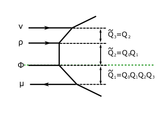
Figure 32: (a): The left strip. (b): The right strip.

The diagram in Figure 32 gives the left strip and the one in Figure 32 gives the right strip. Instead of using the upper half plane with an O5-plane, we write the diagram as a strip diagram by using the mirror image as discussed in section 4.1. Then, the application of the topological vertex to the diagram in Figure 32 yields the result

$$Z^{\rm leftstrip}(\{Q_{i}\};\mu,\nu,\rho,\sigma)=g^{\frac{1}{2}(||\mu||^{2}+||\nu||^{2}+||\rho||^{2})+||\sigma^{t}||^{2}}Z_{\mu}(g)Z_{\nu}(g)Z_{\rho}(g)Z_{\sigma}(g){}^{2}$$ (86)

$$\frac{\mathcal{R}_{\rho\sigma^{t}}(Q_{1})\mathcal{R}_{\nu\sigma^{t}}(Q_{1,2})\mathcal{R}_{\rho\emptyset}(Q_{0,1})\mathcal{R}_{\sigma\sigma}(Q_{0,0})\mathcal{R}_{\mu\sigma^{t}}(Q_{1,2,3})\mathcal{R}_{\nu\emptyset}(Q_{0,1,2})\mathcal{R}_{\mu\emptyset}(Q_{0,1,2,3})}{\mathcal{R}_{\mu\nu^{t}}(Q_{3})\mathcal{R}_{\nu\rho^{t}}(Q_{2})\mathcal{R}_{\mu\rho^{t}}(Q_{2,3})\mathcal{R}_{\rho\sigma}(Q_{0,0,1})\mathcal{R}_{\nu\sigma}(Q_{0,0,1,2})\mathcal{R}_{\mu\sigma}(Q_{0,0,1,2,3})},$$ (87)

where we denote

$$Q_{i,j}=Q_{i}Q_{j},\qquad Q_{i,j,k}=Q_{i}Q_{j}Q_{k},\qquad Q_{i,j,k,\ell}=Q_{i}Q_{j}Q_{k}Q_{\ell},\quad\cdots$$ (88)

for the left strip. As for the right strip, we obtain

$$Z^{\rm rightstrip}(\{\tilde{Q}_{i}\};\mu,\nu,\rho)=g^{\frac{1}{2}(||\mu||^{2}+||\nu^{t}||^{2}+||\rho^{t}||^{2})}Z_{\mu}(g)Z_{\nu}(g)Z_{\rho}(g)$$ (89)

$$\frac{1}{\mathcal{R}_{\nu\rho^{t}}(\tilde{Q}_{3})\mathcal{R}_{\rho\emptyset}(\tilde{Q}_{2})\mathcal{R}_{\emptyset\mu}(\tilde{Q}_{1})\mathcal{R}_{\nu\emptyset}(\tilde{Q}_{2,3})\mathcal{R}_{\rho\mu}(\tilde{Q}_{1,2})\mathcal{R}_{\nu\mu}(\tilde{Q}_{1,2,3})},$$ (90)

with

$$\tilde{Q}_{1}=Q_{0}Q_{1}Q_{2}Q_{3},\qquad\tilde{Q}_{2}=Q_{0}Q_{1},\qquad\tilde{Q}_{3}=Q_{2}.$$ (91)

Note also that the web diagram gives a constraint

$$Q_{3}=Q_{0}Q_{1}.$$ (92)

The full partition function is given by gluing the left strip (86) to the right strip (89) with framing factors and the final result is given by

$$\tilde{Z}_{G_{2},N_{f}=1}= \sum_{\mu,\nu,\rho,\sigma}(+Q_{B}Q_{3}{}^{2})^{|\mu|}(-Q_{B})^{|\nu|+|\rho|}(+Q_{0})^{|\sigma|}f_{\mu}{}^{3}f_{\nu}f_{\rho}{}^{-1}f_{\sigma}$$ (93)

$$Z^{\rm leftstrip}(\{Q_{i}\};\mu,\nu,\rho,\sigma)Z^{\rm rightstrip}(\{\tilde{Q}_{i}\};\mu,\nu,\rho),$$ (94)

where $Q_{B}$ is the K$\ddot{\text{a}}$hler parameter for the bottom color D5-brane in Figure 19. Since the 5-brane web in Figure 19 has parallel external legs. We need to remove an extra factor Bergman:2013ala ; Bao:2013pwa ; Hayashi:2013qwa ; Bergman:2013aca ; Hwang:2014uwa . Hence the partition function after removing the extra factor is

$$Z_{G_{2},N_{f}=1}=\frac{\tilde{Z}_{G_{2},N_{f}=1}}{\mathcal{M}(Q_{0}Q_{1}^{3}Q_{2}^{2}Q_{3})}.$$ (95)

We claim that the partition function (95) is the partition function of the $G_{2}$ gauge theory with one flavor and a singlet.

Since the partition function (95) is still written by the K$\ddot{\text{a}}$hler parameter of the 5-brane web in Figure 32, we will rewrite it by the gauge theory parameters. First the $G_{2}$ gauge theory should have two Coulomb branch moduli $A_{1},A_{2}$ and one instanton fugacity $q$. There is also a mass parameter $M$ for the flavor. Since the one flavor and the singlet both come from the same spinor matter of the $SO(7)$ gauge theory, the mass parameter for the singlet is the same as the mass parameter for the one flavor.

The Coulomb branch parameterization is essentially the same as the parameterization in the case of the pure $G_{2}$ gauge theory. Namely, the Coulomb branch moduli are the height of the color D5-branes. Hence we impose

$$Q_{0}Q_{1}=A_{1},\quad Q_{0}Q_{1}Q_{2}=A_{2}.$$ (96)

Note that the web diagram in Figure 19 has parallel $(1,-1)$ 5-branes. The parallel $(1,-1)$ 5-branes imply an $SU(2)$ flavor symmetry for the one flavor of the $G_{2}$ gauge theory. Therefore, the distance between the two parallel $(1,-1)$ 5-branes is the mass parameter. This leads to a condition

$$Q_{0}Q_{1}^{3}Q_{2}^{2}Q_{3}=M^{2}.$$ (97)

The instanton fugacity can by computed similarly to the way when we calculated the instanton fugacity for the 5d pure $G_{2}$ gauge theory. We extrapolate the leftmost external $(1,-1)$ 5-brane and the external $(2,1)$ 5-brane on the right to the position of the O5-plane in Figure 19 and compute the length between the two extrapolated 5-branes on the O5-plane. In fact it turns out that we need to extrapolate the leftmost external $(1,-1)$ 5-brane instead of the other external $(1,-1)$ 5-brane. This can be justified by the comparison with the instanton fugacity obtained by another 5-brane web digram for the $G_{2}$ gauge theory with one flavor in Figure 17. Then the instanton fugacity is given by

$$Q_{B}Q_{0}^{-1}Q_{1}Q_{2}^{-1}Q_{3}^{-1}=q.$$ (98)

Hence the relations (96), (97), (98) with the condition (92) yields

$$Q_{0}=M^{-1}A_{1}A_{2},\quad Q_{1}=MA_{2}{}^{-1},\quad Q_{2}=A_{1}{}^{-1}A_{2},\quad Q_{B}=qM{}^{-2}A_{1}A_{2}{}^{3}.$$ (99)

Namely, we can compare the partition function (95) with the parameterization (99) with the Nekrasov partition function of the $G_{2}$ gauge theory with one flavor and a singlet.

Perturbative part.

Since $Q_{B}$ is proportional to the instanton fugacity $q$, the perturbative part of the partition function can be obtained by setting $Q_{B}\to 0$. The limit corresponds to the restriction $\mu=\emptyset,\nu=\emptyset,\rho=\emptyset$. In this case, the sum of Young diagrams for the right strip partition function disappears and it reduces to

$$Z^{\text{right}}_{\text{pert}} = \mathcal{M}(\tilde{Q}_{3})\mathcal{M}(\tilde{Q}_{2})\mathcal{M}(\tilde{Q}_{1})\mathcal{M}(\tilde{Q}_{2,3})\mathcal{M}(\tilde{Q}_{1,2})\mathcal{M}(\tilde{Q}_{1,2,3})$$ (100)

$$= \mathcal{M}(A_{1}^{-1}A_{2})\mathcal{M}(A_{1})\mathcal{M}(A_{1}A_{2})\mathcal{M}(A_{2})\mathcal{M}(A_{1}^{2}A_{2})\mathcal{M}(A_{1}A_{2}^{2}).$$

On the other hand, one Young diagram summation remains in the left strip partition function and it becomes

$$Z^{\text{left}}_{\text{pert}} = Z^{\text{left}}_{\text{pert 1}}Z^{\text{left}}_{\text{pert 2}},$$

$$Z^{\text{left}}_{\text{pert 1}} = \frac{\mathcal{M}(Q_{3})\mathcal{M}(Q_{2})\mathcal{M}(Q_{2,3})\mathcal{M}(Q_{0,0,1})\mathcal{M}(Q_{0,0,1,2})\mathcal{M}(Q_{0,0,1,2,3})}{\mathcal{M}(Q_{1})\mathcal{M}(Q_{1,2})\mathcal{M}(Q_{0,1})\mathcal{M}(Q_{0,0})\mathcal{M}(Q_{1,2,3})\mathcal{M}(Q_{0,1,2})\mathcal{M}(Q_{0,1,2,3})},$$ (101)

$$Z^{\text{left}}_{\text{pert 2}} = \sum_{\sigma}Q_{0}^{|\sigma|}f_{\sigma}g^{||\sigma^{t}||^{2}}Z_{\sigma}^{2}(g)\frac{\mathcal{N}_{\emptyset\sigma^{t}}(Q_{1})\mathcal{N}_{\emptyset\sigma^{t}}(Q_{1,2})\mathcal{N}_{\sigma^{t}\sigma}(Q_{0,0})\mathcal{N}_{\emptyset\sigma^{t}}(Q_{1,2,3})}{\mathcal{N}_{\emptyset\sigma}(Q_{0,0,1})\mathcal{N}_{\emptyset\sigma}(Q_{0,0,1,2})\mathcal{N}_{\emptyset\sigma}(Q_{0,0,1,2,3})}.$$ (102)

By the explicit computation of the Young diagram summation of (102), we argue that the partition function (102) becomes

$$Z^{\text{left}}_{\text{pert 2}} = \frac{\mathcal{M}(Q_{0,0})\mathcal{M}(Q_{0,1})\mathcal{M}(Q_{0,1,2})\mathcal{M}(Q_{0,0,1,1,2})\mathcal{M}(Q_{0,1,2,3})\mathcal{M}(Q_{0,0,1,1,2,3})}{\mathcal{M}(Q_{0})\mathcal{M}(Q_{0,0,1})\mathcal{M}(Q_{0,0,1,2})\mathcal{M}(Q_{0,1,1,2})\mathcal{M}(Q_{0,0,1,2,3})\mathcal{M}(Q_{0,1,1,2,3})}$$ (103)

$$\times\frac{\mathcal{M}(Q_{0,0,1,1,2,2,3})\mathcal{M}(Q_{0,1,1,1,2,2,3})}{\mathcal{M}(Q_{0,1,1,2,2,3})\mathcal{M}(Q_{0,0,1,1,1,2,3})}.$$

We checked the equality (103) until the order $Q_{0}^{6}$. Then combining (103) with (101) yields

$$Z^{\text{left}}_{\text{pert}} = \frac{\mathcal{M}(Q_{3})\mathcal{M}(Q_{2})\mathcal{M}(Q_{2,3})\mathcal{M}(Q_{0,0,1,1,2})\mathcal{M}(Q_{0,0,1,1,2,3})\mathcal{M}(Q_{0,0,1,1,2,2,3})\mathcal{M}(Q_{0,1,1,1,2,2,3})}{\mathcal{M}(Q_{1})\mathcal{M}(Q_{1,2})\mathcal{M}(Q_{1,2,3})\mathcal{M}(Q_{0})\mathcal{M}(Q_{0,1,1,2})\mathcal{M}(Q_{0,1,1,2,3})\mathcal{M}(Q_{0,1,1,2,2,3})\mathcal{M}(Q_{0,0,1,1,1,2,2,3})}$$

$$= \frac{\mathcal{M}(A_{1})\mathcal{M}(A_{1}^{-1}A_{2})\mathcal{M}(A_{2})\mathcal{M}(A_{1}A_{2})\mathcal{M}(A_{1}^{2}A_{2})\mathcal{M}(A_{1}A_{2}^{2})\mathcal{M}(M^{2})}{\mathcal{M}(MA_{2}^{-1})\mathcal{M}(MA_{1}^{-1})\mathcal{M}(M)\mathcal{M}(M^{-1}A_{1}A_{2})\mathcal{M}(M)\mathcal{M}(MA_{1})\mathcal{M}(MA_{2})\mathcal{M}(MA_{1}A_{2})}.$$

Therefore, the perturbative part of the partition function of (95) is

$$Z_{\text{pert}} = \frac{Z^{\text{left}}_{\text{pert}}Z^{\text{right}}_{\text{pert}}}{\mathcal{M}(Q_{0}Q_{1}^{3}Q_{2}^{2}Q_{3})}$$

$$= \frac{\mathcal{M}(A_{1})^{2}\mathcal{M}(A_{1}^{-1}A_{2})^{2}\mathcal{M}(A_{2})^{2}\mathcal{M}(A_{1}A_{2})^{2}\mathcal{M}(A_{1}^{2}A_{2})^{2}\mathcal{M}(A_{1}A_{2}^{2})^{2}}{\mathcal{M}(MA_{2}^{-1})\mathcal{M}(MA_{1}^{-1})\mathcal{M}(M)\mathcal{M}(M^{-1}A_{1}A_{2})\mathcal{M}(M)\mathcal{M}(MA_{1})\mathcal{M}(MA_{2})\mathcal{M}(MA_{1}A_{2})}.$$

The perturbative partition function then consists of three factors as follows:

$$Z_{\text{pert}}=Z_{\text{pert}}^{\text{vector}}\cdot Z_{\text{pert}}^{\text{fund}}\cdot Z_{\text{pert}}^{\text{singlet}},$$ (106)

where

$$Z_{\text{pert}}^{\text{vector}} = \mathcal{M}(A_{1})^{2}\mathcal{M}(A_{1}^{-1}A_{2})^{2}\mathcal{M}(A_{2})^{2}\mathcal{M}(A_{1}A_{2})^{2}\mathcal{M}(A_{1}^{2}A_{2})^{2}\mathcal{M}(A_{1}A_{2}^{2})^{2},$$ (107)

$$Z_{\text{pert}}^{\text{fund}} = \frac{1}{\mathcal{M}(MA_{2}^{-1})\mathcal{M}(MA_{1}^{-1})\mathcal{M}(M^{-1}A_{1}A_{2})\mathcal{M}(M)\mathcal{M}(MA_{1})\mathcal{M}(MA_{2})\mathcal{M}(MA_{1}A_{2})},$$

$$Z_{\text{pert}}^{\text{singlet}} = \frac{1}{\mathcal{M}(M)}.$$ (109)

(107), (LABEL:pertflavor) and (109) are exactly equal to the perturbative part of the partition functions of the $G_{2}$ vector multiplets, hypermultiplets in the fundamental representation of $G_{2}$ and a singlet hypermultiplet up to the Cartan parts and flop transitions as in the case of the pure $G_{2}$ gauge theory.

Instanton part.

Let us move on to the instanton part of the $G_{2}$ partition function (95). The instanton part is obtained after removing the perturbative part obtained in (LABEL:pertpart). Namely the instanton partition function of the $G_{2}$ gauge theory with one flavor is

$$Z_{G_{2},N_{f}=1,\text{inst}}=\frac{Z_{G_{2},N_{f}=1}}{Z_{\text{pert}}},$$ (110)

where $Z_{G_{2},N_{f}=1}$ is (95) and $Z_{\text{pert}}$ is (LABEL:pertpart). The order $q^{k}$ of (110) gives the $k$-instanton contribution of the $G_{2}$ gauge theory with one flavor.

Since an explicit form of the instanton partition function of the $G_{2}$ gauge theory with one flavor is not known, we compare the expression (110) with the instanton partition function of the pure $G_{2}$ gauge theory after decoupling the flavor. After sending $M\to 0$, then the 5-brane web diagram will become the one for the pure $G_{2}$ gauge theory in Figure 9. Hence, $Q_{0}Q_{1},Q_{2},Q_{B}$ are still finite in the limit and the instanton fugacity for the pure $G_{2}$ gauge theory is given by $q^{\prime}=qM^{-2}$. Since the limit $M\to 0$ should be compatible with the expansion of $Q_{0}$ in (110) for the comparison, we will take the following steps. At each order of $q^{\prime}$, we first rewrite (110) by $M,A_{1}$ and $Q_{2}$ and then expand it by $M$ and $A_{1}$. In this case, the term $Q_{B}^{k}Q_{0}^{a}Q_{1}^{b}$ becomes

$$Q_{B}^{k}Q_{0}^{a}Q_{1}^{b}=q^{\prime k}M^{-a+b}A_{1}^{2a-b+4k}Q_{2}^{a-b+3k}$$ (111)

The term which survives after the limit $M\to 0$ satisfies $a=b$. In order to obtain an reliable expression until the order $q^{\prime k}A_{1}^{a+4k}$, we need to sum up the Young diagrams in (110) until the order $Q_{0}^{a}Q_{B}^{k}$. Then we can compare the result which is expanded by $A_{1}$ with the gauge theory computation for the pure $G_{2}$ gauge theory. We checked that the partition function (110) after applying the limit $M\to 0$ indeed agrees with the gauge theory result until $a=6$ for the one-instanton and the two-instanton parts of the Nekrasov partition function of the pure $G_{2}$ gauge theory obtained in Benvenuti:2010pq ; Keller:2011ek ; Hanany:2012dm ; Keller:2012da ; Cremonesi:2014xha . This gives an evidence that we obtain the correct the partition function (110) for the $G_{2}$ gauge theory with one flavor.

5 Conclusion

In this paper, we studied 5d $\mathcal{N}=1$ $G_{2}$ gauge theories from 5-brane web diagrams with an O5-plane in type IIB string theory. The result that we obtained is summarized as follows:

• Two equivalent types of 5-brane webs for 5d pure $G_{2}$ gauge theory are presented, in Figures 9, 10, and in Figure 25. Webs for 5d $G_{2}$ gauge theory with matter are also discussed in subsection 2.4.

• Based on the 5-brane webs that we obtained, we computed the partition functions of the BPS spectrum. In particular, the partition function for the pure $G_{2}$ theory is given in (61), and the $G_{2}$ theory with one flavor is given in (95).

For the first type of pure $G_{2}$ diagram, corresponding to Figures 9 and 10, we started from a conventional 5-brane web diagram for the 5d $SO(7)$ gauge theory with a hypermultiplet in the spinor representation. Applying a generalized flop transition such as in Figure 8, we perform a Higgsing associated to the spinor matter to obtain a 5-brane web diagram for the 5d pure $G_{2}$ gauge theory. The detail discussion regarding two diagrams is presented in section 2.

For the second type of pure $G_{2}$ diagram, corresponding to Figure 25, we started with a 5-brane configuration for 5d $SO(8)$ gauge theory with a hypermultiplet in the spinor representation and a hypermultiplet in the conjugate spinor representation. We made use of triality of $SO(8)$ gauge theory so that one can interpret this configuration as 5d $SO(8)$ gauge theory with a vector and a spinor rather than a spinor and a conjugate spinor. With this, we performed a successive Higgsing associated with the vector and the spinor to obtain another 5-brane web for pure $G_{2}$ theory, which is of an O5-plane only.

Our results are tested in two different ways:

• Based on the webs, we computed the tension of monopole strings and compared it with the tension of monopole strings obtained from derivatives of the prepotential of 5d $G_{2}$ gauge theories. They completely agree as shown in (36) and (37).

• For pure $G_{2}$ case, we explicitly compared both the perturbative and instanton parts of the obtained pure $G_{2}$ partition function with the literature. For one flavor case, however, as an explicit expression for the partition function for $G_{2}$ theory with one flavor is not known, we instead checked an important consistency. Namely, the flavor decoupling limit of the instanton part for the $G_{2}$ gauge theory with one flavor reproduces that for the pure $G_{2}$ gauge theory.

Regarding the 5-brane web for pure $G_{2}$ gauge theory, it is worth noting that the 5-brane diagram of the second type has an interesting feature. The diagram is almost identical to the diagram for the pure $SU(4)$ gauge theory of Chern-Simons level zero with a restriction of the Coulomb branch moduli. From the point of view of the topological string computation, the only difference between this $G_{2}$ gauge theory and the pure $SU(4)$ gauge theory is whether a Young diagram is transposed or not. This means that the (unrefined) partition function computations only differ by whether the power of the framing factor is $+1$ or $-1$, and also by whether an associated sign factor is included or not. It would be interesting to see how this feature is modified when one fully refines the $G_{2}$ partition functions HKLY .

As the topological vertex formalism is now applicable to a large class of 5-brane webs with an O5-plane or an $\widetilde{\text{O5}}$-plane, it would be interesting to see whether one can use this method to compute partition functions of 5d $SO(N)$ gauge theories with spinors HKLY . Another direction to pursue is to obtain 5d Seiberg-Witten curves dictating M5-brane configurations based on their dual diagrams HKLY .

- (1) N. Seiberg, Five-dimensional SUSY field theories, nontrivial fixed points and string dynamics, Phys.Lett. B388 (1996) 753–760, [hep-th/9608111].
- (2) D. R. Morrison and N. Seiberg, Extremal transitions and five-dimensional supersymmetric field theories, Nucl.Phys. B483 (1997) 229–247, [hep-th/9609070].
- (3) M. R. Douglas, S. H. Katz, and C. Vafa, Small instantons, Del Pezzo surfaces and type I-prime theory, Nucl.Phys. B497 (1997) 155–172, [hep-th/9609071].
- (4) K. A. Intriligator, D. R. Morrison, and N. Seiberg, Five-dimensional supersymmetric gauge theories and degenerations of Calabi-Yau spaces, Nucl.Phys. B497 (1997) 56–100, [hep-th/9702198].
- (5) O. Aharony and A. Hanany, Branes, superpotentials and superconformal fixed points, Nucl.Phys. B504 (1997) 239–271, [hep-th/9704170].
- (6) O. Aharony, A. Hanany, and B. Kol, Webs of (p,q) five-branes, five-dimensional field theories and grid diagrams, JHEP 9801 (1998) 002, [hep-th/9710116].
- (7) I. Brunner and A. Karch, Branes and six-dimensional fixed points, Phys. Lett. B409 (1997) 109–116, [hep-th/9705022].
- (8) O. Bergman and G. Zafrir, 5d fixed points from brane webs and O7-planes, arXiv:1507.03860.
- (9) H. Hayashi, S.-S. Kim, K. Lee, M. Taki, and F. Yagi, More on 5d descriptions of 6d SCFTs, JHEP 10 (2016) 126, [arXiv:1512.08239].
- (10) G. Zafrir, Brane webs and -planes, JHEP 03 (2016) 109, [arXiv:1512.08114].
- (11) H. Hayashi, S.-S. Kim, K. Lee, and F. Yagi, 6d SCFTs, 5d Dualities and Tao Web Diagrams, arXiv:1509.03300.
- (12) H. Hayashi, S.-S. Kim, K. Lee, and F. Yagi, Equivalence of several descriptions for 6d SCFT, JHEP 01 (2017) 093, [arXiv:1607.07786].
- (13) Y. Yun, Testing 5d-6d dualities with fractional D-branes, JHEP 12 (2016) 016, [arXiv:1607.07615].
- (14) D. Gaiotto and H.-C. Kim, Duality walls and defects in 5d N=1 theories, arXiv:1506.03871.
- (15) G. Zafrir, Brane webs in the presence of an O5−-plane and 4d class S theories of type D, JHEP 07 (2016) 035, [arXiv:1602.00130].
- (16) H. Hayashi, S.-S. Kim, K. Lee, and F. Yagi, Discrete theta angle from an O5-plane, arXiv:1707.07181.
- (17) M. Aganagic, A. Klemm, M. Marino, and C. Vafa, The Topological vertex, Commun.Math.Phys. 254 (2005) 425–478, [hep-th/0305132].
- (18) A. Iqbal, C. Kozcaz, and C. Vafa, The Refined topological vertex, JHEP 0910 (2009) 069, [hep-th/0701156].
- (19) H. Awata and H. Kanno, Refined BPS state counting from Nekrasov’s formula and Macdonald functions, Int.J.Mod.Phys. A24 (2009) 2253–2306, [arXiv:0805.0191].
- (20) N. C. Leung and C. Vafa, Branes and toric geometry, Adv.Theor.Math.Phys. 2 (1998) 91–118, [hep-th/9711013].
- (21) F. Benini, S. Benvenuti, and Y. Tachikawa, Webs of five-branes and N=2 superconformal field theories, JHEP 0909 (2009) 052, [arXiv:0906.0359].
- (22) H. Hayashi, H.-C. Kim, and T. Nishinaka, Topological strings and 5d partition functions, JHEP 1406 (2014) 014, [arXiv:1310.3854].
- (23) H. Hayashi and G. Zoccarato, Exact partition functions of Higgsed 5d theories, JHEP 1501 (2015) 093, [arXiv:1409.0571].
- (24) H. Hayashi and G. Zoccarato, Topological vertex for Higgsed 5d theories, arXiv:1505.00260.
- (25) S.-S. Kim, M. Taki, and F. Yagi, Tao Probing the End of the World, PTEP 2015 (2015), no. 8 083B02, [arXiv:1504.03672].
- (26) H. Hayashi and G. Zoccarato, Partition functions of web diagrams with an O7−-plane, JHEP 03 (2017) 112, [arXiv:1609.07381].
- (27) S.-S. Kim and F. Yagi, Topological vertex formalism with O5-plane, Phys. Rev. D97 (2018) 026011, [arXiv:1709.01928].
- (28) S. Benvenuti, A. Hanany, and N. Mekareeya, The Hilbert Series of the One Instanton Moduli Space, JHEP 06 (2010) 100, [arXiv:1005.3026].
- (29) C. A. Keller, N. Mekareeya, J. Song, and Y. Tachikawa, The ABCDEFG of Instantons and W-algebras, JHEP 03 (2012) 045, [arXiv:1111.5624].
- (30) A. Hanany, N. Mekareeya, and S. S. Razamat, Hilbert Series for Moduli Spaces of Two Instantons, JHEP 01 (2013) 070, [arXiv:1205.4741].
- (31) C. A. Keller and J. Song, Counting Exceptional Instantons, JHEP 07 (2012) 085, [arXiv:1205.4722].
- (32) S. Cremonesi, G. Ferlito, A. Hanany, and N. Mekareeya, Coulomb Branch and The Moduli Space of Instantons, JHEP 12 (2014) 103, [arXiv:1408.6835].
- (33) H.-C. Kim, J. Kim, S. Kim, K.-H. Lee, and J. Park, 6d strings and exceptional instantons, arXiv:1801.03579.
- (34) N. J. Evans, C. V. Johnson, and A. D. Shapere, Orientifolds, branes, and duality of 4-D gauge theories, Nucl. Phys. B505 (1997) 251–271, [hep-th/9703210].
- (35) A. Giveon and D. Kutasov, Brane dynamics and gauge theory, Rev. Mod. Phys. 71 (1999) 983–1084, [hep-th/9802067].
- (36) B. Feng and A. Hanany, Mirror symmetry by O3 planes, JHEP 11 (2000) 033, [hep-th/0004092].
- (37) G. Bertoldi, B. Feng, and A. Hanany, The Splitting of branes on orientifold planes, JHEP 04 (2002) 015, [hep-th/0202090].
- (38) A. Hanany and E. Witten, Type IIB superstrings, BPS monopoles, and three-dimensional gauge dynamics, Nucl.Phys. B492 (1997) 152–190, [hep-th/9611230].
- (39) G. Zafrir, Instanton operators and symmetry enhancement in 5d supersymmetric USp, SO and exceptional gauge theories, JHEP 07 (2015) 087, [arXiv:1503.08136].
- (40) P. Jefferson, H.-C. Kim, C. Vafa, and G. Zafrir, Towards Classification of 5d SCFTs: Single Gauge Node, arXiv:1705.05836.
- (41) A. Iqbal and A.-K. Kashani-Poor, The Vertex on a strip, Adv.Theor.Math.Phys. 10 (2006) 317–343, [hep-th/0410174].
- (42) O. Bergman, D. Rodríguez-Gómez, and G. Zafrir, Discrete and the 5d superconformal index, JHEP 1401 (2014) 079, [arXiv:1310.2150].
- (43) L. Bao, V. Mitev, E. Pomoni, M. Taki, and F. Yagi, Non-Lagrangian Theories from Brane Junctions, JHEP 1401 (2014) 175, [arXiv:1310.3841].
- (44) O. Bergman, D. Rodríguez-Gómez, and G. Zafrir, 5-Brane Webs, Symmetry Enhancement, and Duality in 5d Supersymmetric Gauge Theory, JHEP 1403 (2014) 112, [arXiv:1311.4199].
- (45) C. Hwang, J. Kim, S. Kim, and J. Park, General instanton counting and 5d SCFT, JHEP 07 (2015) 063, [arXiv:1406.6793]. [Addendum: JHEP04,094(2016)].
- (46) H. Hayashi, S.-S. Kim, K. Lee, and F. Yagi, Work in progress, .