Central exclusive diffractive production of $p\bar{p}$ pairs
in proton-proton collisions at high energies

Abstract

We consider the central exclusive production of the $p\bar{p}$ in the continuum and via resonances in proton-proton collisions at high energies. We discuss the diffractive mechanism calculated within the tensor-pomeron approach including pomeron, odderon, and reggeon exchanges. The theoretical results are discussed in the context of existing WA102 and ISR experimental data and predictions for planned or current experiments at the RHIC and the LHC are presented. The distribution in ${\rm y}_{diff}$, the rapidity distance between proton and antiproton, is particularly interesting. We find a dip at ${\rm y}_{diff}=0$ for the $p\bar{p}$ production, in contrast to the $\pi^{+}\pi^{-}$ and $K^{+}K^{-}$ production. We predict also the $p\bar{p}$ invariant mass distribution to be less steep than for the pairs of pseudoscalar mesons. We argue that these specific differences for the $p\bar{p}$ production with respect to the pseudoscalar meson pair production can be attributed to the proper treatment of the spin of produced particles. We discuss asymmetries that are due to the interference of $C=+1$ and $C=-1$ amplitudes of $p\bar{p}$ production. We have also calculated the cross section for the $pp\to pp\Lambda\overline{\Lambda}$ reaction. Here, the cross section is smaller but the characteristic feature for $d\sigma/d{\rm y}_{diff}$ is predicted to be similar to $p\bar{p}$ production. The presence of resonances in the $p\bar{p}$ channel may destroy the dip at ${\rm y}_{diff}=0$. This opens the possibility to study diffractively produced resonances. We discuss the observables suited for this purpose.

I Introduction

Diffractive exclusive production of resonances and of dihadron continua are processes with relatively large cross sections, typically of the order of a few $\mu$b or even larger. It is expected that central exclusive production, mediated by double pomeron exchange, is an ideal reaction for the investigation of gluonic bound states (glueballs) of which the existence has not yet been confirmed unambiguously. Observation of glueballs would be a long-awaited confirmation of a crucial prediction of the QCD theory. Such processes were studied extensively at CERN starting from the Intersecting Storage Rings (ISR) experiments Waldi:1983sc ; Akesson:1985rn ; Breakstone:1986xd ; Breakstone:1989ty ; Breakstone:1990at (for a review, see Ref. Albrow:2010yb ) and later at the Omega spectrometer at SPS in the fixed-target WA102 experiment; see e.g. Barberis:1996iq ; Barberis:1997ve ; Barberis:1998ax ; Barberis:1998sr ; Barberis:1999cq ; Barberis:2000em ; Kirk:2000ws . The measurement of two charged pions in $p\bar{p}$ collisions was performed by the CDF Collaboration at the Tevatron Aaltonen:2015uva . In this experiment the outgoing $p$ and $\bar{p}$ were not detected and only two large rapidity gaps, one on each side of the central hadronic system, were required. Thus, the data include also diffractive dissociation of (anti)protons into undetected hadrons. Exclusive reactions are of particular interest since they can be studied in experiments at the LHC by the ALICE, ATLAS, CMS Khachatryan:2017xsi , and LHCb collaborations. At the LHC, in the reactions of interest here, protons are scattered in the forward/backward directions in which relevant detectors are not always present. Recently, there have been several efforts to install and use forward proton detectors. The CMS Collaboration combines efforts with the TOTEM Collaboration while the ATLAS Collaboration may use the ALFA subdetectors; see e.g. Staszewski:2011bg . Also the STAR experiment at the Relativistic Heavy Ion Collider (RHIC) is equipped with such detectors that allow the measurement of forward protons. In this way, the non-exclusive background due to proton breakup could be rejected via the momentum balance constraint Adamczyk:2014ofa ; Sikora:2016evz .

On the theoretical side, the exclusive diffractive dihadron continuum production can be understood as being mainly due to the exchange of two pomerons between the external protons and the centrally produced hadronic system. First calculations in this respect were concerned with the $pp\to pp\pi^{+}\pi^{-}$ reaction Pumplin:1976dm ; Lebiedowicz:2009pj ; Lebiedowicz:2011nb . The Born amplitude was written in terms of pomeron/reggeon exchanges with parameters fixed from phenomenological analyses of $NN$ and $\pi N$ total and elastic scattering. The four-body amplitude was parametrized using the four-momentum transfers squared $t_{1}$, $t_{2}$, and $s_{ij}$, the energies squared in the two-body subsystems. The energy dependence is known from two-body scatterings such as $NN$, $\pi N$, etc. Such calculations make sense for the continuum production of pseudoscalar meson pairs. These model studies were extended also to the $pp\to nn\pi^{+}\pi^{+}$ Lebiedowicz:2010yb and $pp\to ppK^{+}K^{-}$ Lebiedowicz:2011tp reactions and even for the exclusive $\pi^{+}\pi^{-}\pi^{+}\pi^{-}$ continuum production Kycia:2017iij . In reality the Born approximation is usually not sufficient and absorption corrections have to be taken into account; see e.g. Harland-Lang:2013dia ; Lebiedowicz:2015eka . The phenomenological concepts underlying these calculations require further tests and clear phenomenological evidence to be commonly accepted.

In this paper we are concerned with reactions in which the exchange of the soft pomeron plays the most important role. This – still somewhat enigmatic – soft pomeron is a flavorless object. It is often loosely stated that it possesses quantum numbers of the vacuum. This is true for the internal quantum numbers of the pomeron. However, the spin structure of the soft pomeron certainly is not that of the vacuum, i.e. spin 0. We believe that the soft pomeron is best described as an effective rank-2 symmetric-tensor exchange as introduced in Ewerz:2013kda . In Ewerz:2016onn three hypotheses for the soft-pomeron spin structure, effective scalar, vector, and tensor exchange, were discussed and compared to the experimental data on the helicity structure of proton-proton elastic scattering at $\sqrt{s}=200$ GeV and small $|t|$ from the STAR experiment Adamczyk:2012kn . Only the tensor option was shown to be viable, the vector and scalar options for the soft pomeron could be excluded. In Ewerz:2016onn also some remarks on the history of the views of the pomeron spin structure were presented. For the convenience of the reader we repeat here some of the main points concerning the tensor pomeron in its connection to QCD. In Nachtmann:1991ua , one of us made a general investigation of high-energy soft diffractive processes in QCD using functional methods. It was shown there that the resulting soft pomeron could be described as coherent exchange of spin $2+4+6+\ldots$. This is exactly the structure of the tensor pomeron of Ewerz:2013kda ; see Appendix B there. In this way the tensor pomeron of Ewerz:2013kda has good backing in nonperturbative QCD. Also investigations in the framework of the AdS/CFT correspondence prefer a tensor nature for the soft-pomeron exchange Domokos:2009hm ; Iatrakis:2016rvj .

First applications of the tensor-pomeron model of Ewerz:2013kda to the central exclusive production (CEP) of several scalar and pseudoscalar mesons in the reaction $pp\to ppM$ were studied in Lebiedowicz:2013ika for the relatively low WA102 energy, where also the secondary reggeon exchanges play a very important role. The resonant $\rho^{0}$ ($J^{PC}=1^{--}$) and non-resonant (Drell-Söding) $\pi^{+}\pi^{-}$ photoproduction contributions to CEP were studied in Lebiedowicz:2014bea . In Bolz:2014mya , an extensive study of the reaction $\gamma p\to\pi^{+}\pi^{-}p$ was presented. In Lebiedowicz:2016ioh , the model was applied to the reaction $pp\to pp\pi^{+}\pi^{-}$ including the dipion continuum, the dominant scalar $f_{0}(500)$, $f_{0}(980)$ ($J^{PC}=0^{++}$), and tensor $f_{2}(1270)$ ($J^{PC}=2^{++}$) resonances decaying into the $\pi^{+}\pi^{-}$ pairs. In Lebiedowicz:2016zka , the model was applied to the $\pi^{+}\pi^{-}\pi^{+}\pi^{-}$ production via the intermediate $\sigma\sigma$ and $\rho^{0}\rho^{0}$ states. Also the $\rho^{0}$ meson production associated with a very forward/backward $\pi N$ system, that is, the $pp\to pp\rho^{0}\pi^{0}$ and $pp\to pn\rho^{0}\pi^{+}$ processes were discussed in Lebiedowicz:2016ryp . It was shown in Lebiedowicz:2013ika ; Lebiedowicz:2016ioh ; Lebiedowicz:2014bea ; Bolz:2014mya ; Lebiedowicz:2016ryp ; Lebiedowicz:2016zka that the tensor-pomeron model does quite well in reproducing the data where available.

Closely related to the reaction $pp\to ppp\bar{p}$ studied by us here are the reactions of central $p\bar{p}$ production in ultraperipheral nucleus-nucleus and nucleon-nucleus collisions, $AA\to AAp\bar{p}$ and $pA\to pAp\bar{p}$. For the first process, see Klusek-Gawenda:2017lgt , in which the parameters of the model including the proton exchange, the $f_{2}(1270)$ and $f_{2}(1950)$ $s$-channel exchanges, and the handbag mechanism, were fitted to Belle data Kuo:2005nr for the $\gamma\gamma\to p\bar{p}$ reaction. The model was applied then to estimate the cross section for the ultraperipheral, ultrarelativistic, heavy-ion collisions at the LHC.

In the following, we extend the application of the tensor-pomeron model to central exclusive production of spin-$1/2$ hadron pairs ($p\bar{p}$ or $\Lambda\overline{\Lambda}$) in $pp$ collisions. The centrally produced baryon-antibaryon pairs were studied experimentally in Refs. Akesson:1985rn ; Breakstone:1989ty ; Barberis:1998sr . So far, the $pp\to ppp\bar{p}$ reaction at LHC energies has not been considered from the theory point of view. We will show first predictions for this reaction in the tensor-pomeron approach and compare them with results for central production of dihadrons with spin 0, $\pi^{+}\pi^{-}$ and $K^{+}K^{-}$. We shall discuss whether the predictions of the tensor-pomeron model can be verified by planned measurements at the RHIC and at the LHC. The observables suited for this purpose shall be presented.

Our paper is organised as follows. In Sec. II we discuss continuum $p\bar{p}$ production. Section III deals with $p\bar{p}$ production via scalar resonances. First results are presented in Sec. IV, and Sec. V presents our conclusions. We include in our calculations the exchanges of the soft pomeron, of reggeons, and also of the soft odderon for some distributions. The odderon was introduced a long time ago Lukaszuk:1973nt ; Joynson:1975az (for a review, see, e.g. Ewerz:2003xi ) and has recently become very interesting again Antchev:2017yns ; Martynov:2017zjz ; Khoze:2017swe ; Khoze:2018bus .

We want to emphasise that the purpose of our paper is not to compare predictions of our tensor-pomeron approach with alternatives for the soft-pomeron structure. This has been done extensively in Lebiedowicz:2013ika ; Ewerz:2016onn . Also, since we are interested in the soft-scattering regime we cannot use or compare with the perturbative pomeron, initiated in Low:1975sv ; Nussinov:1975mw ; Kuraev:1977fs ; Balitsky:1978ic . The purpose of our work is to give experimentalists a solid idea of what to expect theoretically in central exclusive $p\bar{p}$ production. What are the magnitudes of cross sections? Where is continuum $p\bar{p}$? Where is resonance production prominent? What is the role of secondary reggeon exchanges and, if it exists, of odderon exchange? What are the differences between $p\bar{p}$ and two pseudoscalars central production? We would hope that our calculations could serve as basis for the construction of an event generator for this and related processes. A long-term goal would be to derive the coupling constants of our effective theory from nonperturbative QCD, but this is beyond the scope of the present paper.

II $p\bar{p}$ continuum production

We study central exclusive production of $p\bar{p}$ in proton-proton collisions at high energies

$$p(p_{a},\lambda_{a})+p(p_{b},\lambda_{b})\to p(p_{1},\lambda_{1})+\bar{p}(p_{3},\lambda_{3})+p(p_{4},\lambda_{4})+p(p_{2},\lambda_{2})\,,$$ (1)

where $p_{i}$ and $\lambda_{i}\in\{+1/2,-1/2\}$, indicated in brackets, denote the 4-momenta and helicities of the nucleons, respectively. The ${\cal T}$-matrix element for the reaction (1) will be denoted as follows

$$\begin{split}{\cal M}_{\lambda_{a}\lambda_{b}\to\lambda_{1}\lambda_{2}\lambda_{3}\lambda_{4}}=\langle p(p_{1},\lambda_{1}),p(p_{4},\lambda_{4}),\bar{p}(p_{3},\lambda_{3})p(p_{2},\lambda_{2})|{\cal T}&|p(p_{a},\lambda_{a}),p(p_{b},\lambda_{b})\rangle\,.\end{split}$$ (2)

Note that the order of the particles in the bra and ket states matters since we are dealing with fermions.

In general the full amplitude for the $p\bar{p}$ production is a sum of the continuum amplitude and the amplitudes with the $s$-channel resonances:

$$\begin{split}{\cal M}_{\lambda_{a}\lambda_{b}\to\lambda_{1}\lambda_{2}\lambda_{3}\lambda_{4}}={\cal M}^{p\bar{p}{\rm-continuum}}_{\lambda_{a}\lambda_{b}\to\lambda_{1}\lambda_{2}\lambda_{3}\lambda_{4}}+{\cal M}^{p\bar{p}{\rm-resonances}}_{\lambda_{a}\lambda_{b}\to\lambda_{1}\lambda_{2}\lambda_{3}\lambda_{4}}\,.\end{split}$$ (3)

At high energies the exchange objects to be considered are the photon $\gamma$, the pomeron $\mathbb{P}$, the odderon $\mathbb{O}$, and the reggeons $\mathbb{R}$. Their charge conjugation and $G$-parity quantum numbers are listed in Table I of Lebiedowicz:2016ioh . We treat the $C=+1$ pomeron and the reggeons $\mathbb{R}_{+}=f_{2\mathbb{R}},a_{2\mathbb{R}}$ as effective tensor exchanges while the $C=-1$ odderon and the reggeons $\mathbb{R}_{-}=\omega_{\mathbb{R}},\rho_{\mathbb{R}}$ are treated as effective vector exchanges.

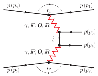
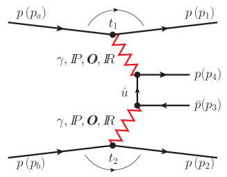
Figure 1: The Born diagrams for the double pomeron/reggeon and photon-mediated central exclusive continuum $p\bar{p}$ production in proton-proton collisions.

The $p\bar{p}$ continuum amplitude is expressed as the sum of ${\rm\hat{t}}$ and ${\rm\hat{u}}$ diagrams shown in Fig. 1,

$${\cal M}^{p\bar{p}-\rm{continuum}}_{\lambda_{a}\lambda_{b}\to\lambda_{1}\lambda_{2}\lambda_{3}\lambda_{4}}={\cal M}^{({\rm\hat{t}})}_{\lambda_{a}\lambda_{b}\to\lambda_{1}\lambda_{2}\lambda_{3}\lambda_{4}}+{\cal M}^{({\rm\hat{u}})}_{\lambda_{a}\lambda_{b}\to\lambda_{1}\lambda_{2}\lambda_{3}\lambda_{4}}\,.$$ (4)

The combinations $(C_{1},C_{2})$ of exchanges that can contribute in (4) are

$$(C_{1},C_{2})=(1,1):\;(\mathbb{P}+\mathbb{R}_{+},\mathbb{P}+\mathbb{R}_{+})\,;$$ (5)

$$(C_{1},C_{2})=(-1,-1):\;(\mathbb{O}+\mathbb{R}_{-}+\gamma,\mathbb{O}+\mathbb{R}_{-}+\gamma)\,;$$ (6)

$$(C_{1},C_{2})=(1,-1):\;(\mathbb{P}+\mathbb{R}_{+},\mathbb{O}+\mathbb{R}_{-}+\gamma)\,;$$ (7)

$$(C_{1},C_{2})=(-1,1):\;(\mathbb{O}+\mathbb{R}_{-}+\gamma,\mathbb{P}+\mathbb{R}_{+})\,.$$ (8)

Here $C_{1}$ and $C_{2}$ are the charge-conjugation quantum numbers of the exchange objects. The contributions involving the photon $\gamma$ in (6) to (8) are expected to be small but may be important at very small four-momentum transfer squared. The $(\gamma,\mathbb{P}+\mathbb{R}_{+})$ and $(\mathbb{P}+\mathbb{R}_{+},\gamma)$ contributions will be very important for the $p\bar{p}$ production in $pA$ collisions. There one also has to take into account contact terms required by gauge invariance. This will be studied elsewhere. The contributions involving the odderon $\mathbb{O}$ are expected to be small since its coupling to the proton is very small. Thus, we shall concentrate on the diffractive production of $p\bar{p}$ through the $\mathbb{P}$, $\mathbb{R}_{+}$, and $\mathbb{R}_{-}$ exchanges but also mention odderon effects where appropriate.

The kinematic variables for reaction (1) are

$$s=(p_{a}+p_{b})^{2}=(p_{1}+p_{2}+p_{3}+p_{4})^{2}\,,$$

$$s_{ij}=(p_{i}+p_{j})^{2},\quad s_{34}=M_{34}^{2}=(p_{3}+p_{4})^{2}\,,$$

$$t_{1}=q_{1}^{2},\quad q_{1}=p_{a}-p_{1}\,,$$

$$t_{2}=q_{2}^{2},\quad q_{2}=p_{b}-p_{2}\,,$$

$$\hat{p}_{t}=p_{a}-p_{1}-p_{3}\,,$$

$$\hat{p}_{u}=p_{4}-p_{a}+p_{1}\,.$$ (9)

Let us first take a look at the dominant ($\mathbb{P}$, $\mathbb{P}$) contribution. The ${\rm\hat{t}}$- and ${\rm\hat{u}}$-channel amplitudes for the $\mathbb{P}\mathbb{P}$-exchange can be written as

$$\begin{split}&{\cal M}^{({\rm\hat{t}})}_{\lambda_{a}\lambda_{b}\to\lambda_{1}\lambda_{2}\lambda_{3}\lambda_{4}}=(-i)\bar{u}(p_{1},\lambda_{1})i\Gamma^{(\mathbb{P}pp)}_{\mu_{1}\nu_{1}}(p_{1},p_{a})u(p_{a},\lambda_{a})\;i\Delta^{(\mathbb{P})\,\mu_{1}\nu_{1},\alpha_{1}\beta_{1}}(s_{13},t_{1})\\ &\qquad\qquad\qquad\quad\times\bar{u}(p_{4},\lambda_{4})\,i\Gamma^{(\mathbb{P}pp)}_{\alpha_{2}\beta_{2}}(p_{4},\hat{p}_{t})\,iS_{F}(\hat{p}_{t})\,i\Gamma^{(\mathbb{P}pp)}_{\alpha_{1}\beta_{1}}(\hat{p}_{t},-p_{3})\,v(p_{3},\lambda_{3})\\ &\qquad\qquad\qquad\quad\times i\Delta^{(\mathbb{P})\,\alpha_{2}\beta_{2},\mu_{2}\nu_{2}}(s_{24},t_{2})\,\bar{u}(p_{2},\lambda_{2})i\Gamma^{(\mathbb{P}pp)}_{\mu_{2}\nu_{2}}(p_{2},p_{b})u(p_{b},\lambda_{b})\,,\end{split}$$ (10)

$$\begin{split}&{\cal M}^{({\rm\hat{u}})}_{\lambda_{a}\lambda_{b}\to\lambda_{1}\lambda_{2}\lambda_{3}\lambda_{4}}=(-i)\bar{u}(p_{1},\lambda_{1})i\Gamma^{(\mathbb{P}pp)}_{\mu_{1}\nu_{1}}(p_{1},p_{a})u(p_{a},\lambda_{a})\;i\Delta^{(\mathbb{P})\,\mu_{1}\nu_{1},\alpha_{1}\beta_{1}}(s_{14},t_{1})\\ &\qquad\qquad\qquad\quad\times\bar{u}(p_{4},\lambda_{4})\,i\Gamma^{(\mathbb{P}pp)}_{\alpha_{1}\beta_{1}}(p_{4},\hat{p}_{u})\,iS_{F}(\hat{p}_{u})\,i\Gamma^{(\mathbb{P}pp)}_{\alpha_{2}\beta_{2}}(\hat{p}_{u},-p_{3})\,v(p_{3},\lambda_{3})\\ &\qquad\qquad\qquad\quad\times i\Delta^{(\mathbb{P})\,\alpha_{2}\beta_{2},\mu_{2}\nu_{2}}(s_{23},t_{2})\,\bar{u}(p_{2},\lambda_{2})i\Gamma^{(\mathbb{P}pp)}_{\mu_{2}\nu_{2}}(p_{2},p_{b})u(p_{b},\lambda_{b})\,.\end{split}$$ (11)

Here we use the standard propagator for the proton $iS_{F}(\hat{p})=i/(\hat{p}\!\!\!/-m_{p})$. The effective propagator of the tensor-pomeron exchange and the pomeron-proton vertex function are given in section 3 of Ewerz:2013kda . For the convenience of the reader we collect these and other quantities which we use in our work in Appendix A.

For $\mathbb{P}\mathbb{P}$ fusion the centrally produced $p\bar{p}$ system is in a state of $C=+1$. This implies for the amplitude (2) the following:

$$\begin{split}&\langle p(p_{1},\lambda_{1}),p(p_{4},\lambda_{4}),\bar{p}(p_{3},\lambda_{3}),p(p_{2},\lambda_{2})|{\cal T}|p(p_{a},\lambda_{a}),p(p_{b},\lambda_{b})\rangle^{(\mathbb{P},\mathbb{P})}\\ &=\langle p(p_{1},\lambda_{1}),\bar{p}(p_{4},\lambda_{4}),p(p_{3},\lambda_{3}),p(p_{2},\lambda_{2})|{\cal T}|p(p_{a},\lambda_{a}),p(p_{b},\lambda_{b})\rangle^{(\mathbb{P},\mathbb{P})}\\ &=-\langle p(p_{1},\lambda_{1}),p(p_{3},\lambda_{3}),\bar{p}(p_{4},\lambda_{4}),p(p_{2},\lambda_{2})|{\cal T}|p(p_{a},\lambda_{a}),p(p_{b},\lambda_{b})\rangle^{(\mathbb{P},\mathbb{P})}\,.\end{split}$$ (12)

Here, we work in the overall c.m. system and assume that the helicity states for the centrally produced $p$ and $\bar{p}$ are both taken of the same type, e.g., of type (a); see Appendix A of Klusek-Gawenda:2017lgt . This antisymmetry relation (12) can, of course, be verified explicitly using the expressions for ${\cal M}^{({\rm\hat{t}})}$ and ${\cal M}^{({\rm\hat{u}})}$ from (10) and (11), respectively.

If we use another choice of $p$ and $\bar{p}$ helicity states in the c.m. system we will get additional phase factors in (12) and the corresponding relations for the other $(C_{1},C_{2})$ exchanges. But these phase factors drop out for distributions where the polarisations of the centrally produced $p$ and $\bar{p}$ are not observed. Thus, our above choice for the $p$ and $\bar{p}$ helicity states is very convenient as it makes the $p\bar{p}$ charge-conjugation relations for the amplitudes simple and explicit.

The antisymmetry relation (12) holds for all exchanges with $(C_{1},C_{2})$ = $(1,1)$ and $(-1,-1)$; see (5) and (6). For the exchanges with $(C_{1},C_{2})$ = $(1,-1)$ and $(-1,1)$ we have, instead, symmetry under the exchange $\left(p(p_{4},\lambda_{4}),\bar{p}(p_{3},\lambda_{3})\right)\to\left(p(p_{3},\lambda_{3}),\bar{p}(p_{4},\lambda_{4})\right)$; see (7) and (8).

In the high-energy approximation, we can write the $\mathbb{P}\mathbb{P}$-exchange amplitude as

$$\begin{split}&{\cal M}^{(\mathbb{P}\mathbb{P}\to p\bar{p})}_{\lambda_{a}\lambda_{b}\to\lambda_{1}\lambda_{2}\lambda_{3}\lambda_{4}}\simeq(3\beta_{\mathbb{P}NN})^{2}\,2(p_{1}+p_{a})_{\mu_{1}}(p_{1}+p_{a})_{\nu_{1}}\,\delta_{\lambda_{1}\lambda_{a}}\,[F_{1}(t_{1})]^{2}\\ &\qquad\qquad\qquad\quad\times\bar{u}(p_{4},\lambda_{4})\Large[\gamma^{\mu_{2}}(p_{4}+\hat{p}_{t})^{\nu_{2}}\,\frac{1}{4s_{13}}(-is_{13}\alpha^{\prime}_{\mathbb{P}})^{\alpha_{\mathbb{P}}(t_{1})-1}\frac{[\hat{F}_{p}(\hat{p}_{t}^{2})]^{2}}{\not\!\hat{p}_{t}-m_{p}}\\ &\qquad\qquad\qquad\quad\times\gamma^{\mu_{1}}(\hat{p}_{t}-p_{3})^{\nu_{1}}\,\frac{1}{4s_{24}}(-is_{24}\alpha^{\prime}_{\mathbb{P}})^{\alpha_{\mathbb{P}}(t_{2})-1}\\ &\qquad\qquad\qquad\qquad+\gamma^{\mu_{1}}(p_{4}+\hat{p}_{u})^{\nu_{1}}\frac{1}{4s_{14}}(-is_{14}\alpha^{\prime}_{\mathbb{P}})^{\alpha_{\mathbb{P}}(t_{1})-1}\frac{[\hat{F}_{p}(\hat{p}_{u}^{2})]^{2}}{\not\!\hat{p}_{u}-m_{p}}\\ &\qquad\qquad\qquad\quad\times\gamma^{\mu_{2}}(\hat{p}_{u}-p_{3})^{\nu_{2}}\,\frac{1}{4s_{23}}(-is_{23}\alpha^{\prime}_{\mathbb{P}})^{\alpha_{\mathbb{P}}(t_{2})-1}\Large]\,v(p_{3},\lambda_{3})\\ &\qquad\qquad\qquad\quad\times(3\beta_{\mathbb{P}NN})^{2}\,2(p_{2}+p_{b})_{\mu_{2}}(p_{2}+p_{b})_{\nu_{2}}\,\delta_{\lambda_{2}\lambda_{b}}\,[F_{1}(t_{2})]^{2}\,.\end{split}$$ (13)

In (13), we have introduced a form factor $\hat{F}_{p}(\hat{p}^{2})$, taking into account that the intermediate protons in Fig. 1 are off shell. This proton off-shell form factor is parametrized here in the exponential form,

$$\hat{F}_{p}(\hat{p}^{2})=\exp\left(\frac{\hat{p}^{2}-m_{p}^{2}}{\Lambda_{off,E}^{2}}\right)\,,$$ (14)

where $\Lambda_{off,E}$ has to be adjusted to experimental data. The form factor (14) is normalized to unity at the on-shell point $\hat{p}^{2}=m_{p}^{2}$.

In a way similar to (10) - (13) we can write the amplitudes for the exchanges $(\mathbb{P},\mathbb{R}_{+})$, $(\mathbb{R}_{+},\mathbb{P})$, and $(\mathbb{R}_{+},\mathbb{R}_{+})$, since both, $\mathbb{P}$ and $\mathbb{R}_{+}$ exchange, are treated as tensor exchanges in our model. The contributions in (6) - (8) involving $C=-1$ exchanges are different. We recall that $\mathbb{R}_{-}$ exchanges are treated as effective vector exchanges in our model; see Sec. 3 of Ewerz:2013kda and Appendix A of the present paper.

III $pp\to pp(f_{0}\to p\bar{p})$

The resonances produced diffractively in the $p\bar{p}$ channel are not well known. Therefore, we will concentrate only on the $s$-channel scalar resonances. We shall study the reaction $pp\to pp(f_{0}\to p\bar{p})$ where $f_{0}$ stands for one of the $f_{0}(2020)$, $f_{0}(2100)$, and $f_{0}(2200)$ states with $I^{G}(J^{PC})=0^{+}(0^{++})$. It must be noted that these states are only listed in Olive:2016xmw and are not included in the summary tables. Also their couplings to the $p\bar{p}$ channel are essentially unknown.

The $\mathbb{P}\mathbb{P}$-exchange amplitude through a scalar resonance $f_{0}\to p\bar{p}$ can be written as

$$\begin{split}&{\cal M}^{(\mathbb{P}\mathbb{P}\to f_{0}\to p\bar{p})}_{\lambda_{a}\lambda_{b}\to\lambda_{1}\lambda_{2}\lambda_{3}\lambda_{4}}\simeq 3\beta_{\mathbb{P}NN}\,2(p_{1}+p_{a})_{\mu_{1}}(p_{1}+p_{a})_{\nu_{1}}\,\delta_{\lambda_{1}\lambda_{a}}\,F_{1}(t_{1})\;\frac{1}{4s_{1}}(-is_{1}\alpha^{\prime}_{\mathbb{P}})^{\alpha_{\mathbb{P}}(t_{1})-1}\\ &\quad\quad\times\Gamma^{(\mathbb{P}\mathbb{P}f_{0})\,\mu_{1}\nu_{1},\mu_{2}\nu_{2}}(q_{1},q_{2})\,\Delta^{(f_{0})}(p_{34})\,\bar{u}(p_{4},\lambda_{4})\,\Gamma^{(f_{0}p\bar{p})}(p_{4},-p_{3})\,v(p_{3},\lambda_{3})\\ &\quad\quad\times\frac{1}{4s_{2}}(-is_{2}\alpha^{\prime}_{\mathbb{P}})^{\alpha_{\mathbb{P}}(t_{2})-1}\,3\beta_{\mathbb{P}NN}\,2(p_{2}+p_{b})_{\mu_{2}}(p_{2}+p_{b})_{\nu_{2}}\,\delta_{\lambda_{2}\lambda_{b}}\,F_{1}(t_{2})\,,\end{split}$$ (15)

where $s_{1}=(p_{1}+p_{3}+p_{4})^{2}$, $s_{2}=(p_{2}+p_{3}+p_{4})^{2}$, and $p_{34}=p_{3}+p_{4}$.

The effective Lagrangians and the vertices for $\mathbb{P}\mathbb{P}$ fusion into an $f_{0}$ meson are discussed in Appendix A of Lebiedowicz:2013ika . As was shown there the tensorial $\mathbb{P}\mathbb{P}f_{0}$ vertex corresponds to the sum of the two lowest values of $(l,S)$, that is, $(l,S)=(0,0)$ and $(2,2)$ with coupling parameters $g_{\mathbb{P}\mathbb{P}f_{0}}^{\prime}$ and $g_{\mathbb{P}\mathbb{P}f_{0}}^{\prime\prime}$, respectively. The vertex, including a form factor, reads then as follows ($p_{34}=q_{1}+q_{2}$):

$$i\Gamma_{\mu\nu,\kappa\lambda}^{(\mathbb{P}\mathbb{P}f_{0})}(q_{1},q_{2})=\left(i\Gamma_{\mu\nu,\kappa\lambda}^{\prime(\mathbb{P}\mathbb{P}f_{0})}\mid_{bare}+i\Gamma_{\mu\nu,\kappa\lambda}^{\prime\prime(\mathbb{P}\mathbb{P}f_{0})}(q_{1},q_{2})\mid_{bare}\right)\tilde{F}^{(\mathbb{P}\mathbb{P}f_{0})}(q_{1}^{2},q_{2}^{2},p_{34}^{2})\,;$$ (16)

see Eq. (A.21) of Lebiedowicz:2013ika . As was shown in Lebiedowicz:2013ika these two $(l,S)$ couplings give different results for the distribution in the azimuthal angle between the transverse momenta $\vec{p}_{t,1}$ and $\vec{p}_{t,2}$ of the outgoing leading protons. We take the factorized form for the pomeron-pomeron-meson form factor

$$\tilde{F}^{(\mathbb{P}\mathbb{P}f_{0})}(q_{1}^{2},q_{2}^{2},p_{34}^{2})=F_{M}(q_{1}^{2})F_{M}(q_{2}^{2})F^{(\mathbb{P}\mathbb{P}f_{0})}(p_{34}^{2})\,$$ (17)

normalised to $\tilde{F}^{(\mathbb{P}\mathbb{P}f_{0})}(0,0,m_{f_{0}}^{2})=1$. We will further set

$$F^{(\mathbb{P}\mathbb{P}f_{0})}(p_{34}^{2})=\exp{\left(\frac{-(p_{34}^{2}-m_{f_{0}}^{2})^{2}}{\Lambda_{f_{0}}^{4}}\right)}\,,\quad\Lambda_{f_{0}}=1\;{\rm GeV}\,.$$ (18)

The scalar-meson propagator is taken as

$$i\Delta^{(f_{0})}(p_{34})=\dfrac{i}{p_{34}^{2}-m_{f_{0}}^{2}+im_{f_{0}}\Gamma_{f_{0}}}\,,$$ (19)

with constant widths for the $f_{0}$ states with the numerical values from Olive:2016xmw .

For the $f_{0}p\bar{p}$ vertex we have

$$i\Gamma^{(f_{0}p\bar{p})}(p_{4},-p_{3})=ig_{f_{0}p\bar{p}}\,F^{(f_{0}p\bar{p})}(p_{34}^{2})\,,$$ (20)

where $g_{f_{0}p\bar{p}}$ is an unknown dimensionless parameter. We assume $g_{f_{0}p\bar{p}}>0$ and $F^{(f_{0}p\bar{p})}(p_{34}^{2})$ = $F^{(\mathbb{P}\mathbb{P}f_{0})}(p_{34}^{2})$; see Eq. (18).

IV First results

We start our analysis by comparing the cross section of our non-resonant contribution to the $pp\to ppp\bar{p}$ reaction (1) with the CERN ISR data at $\sqrt{s}=62$ GeV Breakstone:1989ty . In Breakstone:1989ty the centrally produced antiproton and proton were restricted to lie in the rapidity regions $|{\rm y}_{3}|$, $|{\rm y}_{4}|<1.5$, respectively, and the outgoing forward protons to have $x_{F,p}>0.9$ and the four-momentum transfer squared $|t|\geqslant 0.08$ GeV². With such kinematic conditions we get the integrated cross section of $\sigma_{th}=0.013$ and 0.236 $\mu$b for $\Lambda_{off,E}=0.8$ and 1 GeV, respectively, compared with $\sigma_{exp}=0.80\pm 0.17$ $\mu$b from Breakstone:1989ty . Our theoretical results have been obtained in the Born approximation (neglecting absorptive corrections). The realistic cross section can be obtained by multiplying the Born cross section by the corresponding gap survival factor $\langle S^{2}\rangle$. At the ISR energies we estimate it to be $\langle S^{2}\rangle\simeq 0.5$.  In our calculations, we include the pomeron and reggeon $\mathbb{R}_{+}$ and $\mathbb{R}_{-}$ exchanges; see (5) - (8). For double pomeron exchange and $\Lambda_{off,E}=1$ GeV we get only $\sigma_{th}=0.077$ $\mu$b. It is seen that inclusion of subleading reggeon exchanges is crucial at the ISR energy. In Akesson:1985rn the measurement was performed at $\sqrt{s}=63$ GeV, $|{\rm y}_{3}|,|{\rm y}_{4}|\leqslant 1$, $x_{F,p}>0.95$, $0.01\lesssim|t|\lesssim 0.06$ GeV² and the cross section $d^{2}\sigma_{exp}/dt_{1}dt_{2}=1.0\pm 0.5$ $\mu$b GeV^-4 for $t_{1}=t_{2}=-0.035$ GeV² was determined. We get (without absorption) $d^{2}\sigma_{th}/dt_{1}dt_{2}=0.73$ and 14.14 $\mu$b GeV^-4 for $\Lambda_{off,E}=0.8$ and 1 GeV, respectively. We see that this experiment supports the smaller value of $\Lambda_{off,E}$. Although the ISR experiments Akesson:1985rn ; Breakstone:1989ty were performed for different kinematic coverage, in both an enhancement in the low $p\bar{p}$ invariant-mass region was observed. The low-mass enhancement is clearly seen also at the WA102 energy Barberis:1998sr , see Fig. 1 (b) there. Therefore, the non-resonant (continuum) contribution alone is not sufficient to describe the low-energy data and, e.g., scalar and/or tensor resonance contributions should be taken into account. We will return to this issue below (see Fig. 9).

Now we show numerical results for the reaction $pp\to ppp\bar{p}$ at higher energies. In Table 1 we have collected cross sections in $\mu b$ for the exclusive $p\bar{p}$ continuum including some experimental cuts. We show results for the pomeron and reggeon exchanges in the amplitude (see the column “$\mathbb{P}$ and $\mathbb{R}$”) and when only the $(\mathbb{P},\mathbb{P})$ term contributes (see the column “$\mathbb{P}$”). The calculations have been done in the Born approximation (without absorption effects) and for $\Lambda_{off,E}=1$ GeV in (14). The absorption effects lead to a damping of the cross section by a factor 5 for $\sqrt{s}=0.2$ TeV and by a factor 10 for $\sqrt{s}=13$ TeV; see e.g. Lebiedowicz:2015eka . The next-to-last line in Table 1 shows result with an extra cut on leading protons of 0.17 GeV $<|p_{y,1}|,|p_{y,2}|<$ 0.5 GeV that will be measured in ALFA on both sides of the ATLAS detector.

Table 1: The integrated cross sections in $\mu$b for the exclusive diffractive $p\bar{p}$ continuum production for some experimental cuts on (pseudo)rapidity and $p_{t}$ of centrally produced individual $p$ and $\bar{p}$ for the STAR, ALICE, ATLAS, CMS, and LHCb experiments. Results for some limitations on leading protons are also shown. The column “$\mathbb{P}$ and $\mathbb{R}$” shows the resulting total cross sections from $\mathbb{P}$ and $\mathbb{R}$ ($\mathbb{R}_{+}$ and $\mathbb{R}_{-}$) exchanges, which include, of course, the interference term between the various components. The column “$\mathbb{P}$” shows results obtained for the $\mathbb{P}$ exchange alone. We have taken here $\Lambda_{off,E}=1$ GeV. No absorption effects were included here.

$\sqrt{s}$, TeV	Cuts	$\mathbb{P}$ and $\mathbb{R}$	$\mathbb{P}$
0.2	$|\eta|<1$, $p_{t}>0.2$ GeV	0.031	0.018
0.2	$|\eta|<1$, $p_{t}>0.2$ GeV, $0.03<-t_{1,2}<0.3$ GeV2	0.014	0.008
13	$|\eta|<0.9$, $p_{t}>0.1$ GeV	0.032	0.031
13	$|\rm{y}|<2$, $p_{t}>0.2$ GeV	2.38	2.19
13	$|\eta|<2.5$, $p_{t}>0.1$ GeV	1.96	1.82
13	$|\eta|<2.5$, $p_{t}>0.1$ GeV, $0.17<|p_{y}|<0.5$ GeV	0.31	0.29
13	$2<\eta<4.5$, $p_{t}>0.2$ GeV	0.79	0.68

We have also calculated the corresponding cross sections for the $pp\to pp\Lambda\overline{\Lambda}$ reaction, taking into account only the dominant $(\mathbb{P},\mathbb{P})$ contribution. The amplitude ${\cal M}^{(\mathbb{P}\mathbb{P}\to\Lambda\overline{\Lambda})}$ is very much the same as ${\cal M}^{(\mathbb{P}\mathbb{P}\to p\bar{p})}$ (13) but with $m_{p}$, $\hat{F}_{p}$ replaced by $m_{\Lambda}$, $\hat{F}_{\Lambda}$. To describe the off-shellness of the intermediate $t/u$-channel $\Lambda$ baryons we assume the form factor given by Eq. (14) with $\Lambda_{off,E}=1$ GeV. For the coupling of the $\Lambda$ baryon to the pomeron we make an ansatz similar to the proton-pomeron coupling in (31) of Appendix A but with $\beta_{\mathbb{P}NN}$ replaced by a constant $\beta_{\mathbb{P}\Lambda\Lambda}$. The value of the latter can be estimated from the data on the total cross sections for $\Lambda p$ and $pp$ scattering at high energies using (6.41) of Ewerz:2013kda

$$\beta_{\mathbb{P}\Lambda\Lambda}\cong\beta_{\mathbb{P}NN}\frac{\sigma_{tot}(\Lambda p)}{\sigma_{tot}(pp)}\cong 1.87\;{\rm GeV}^{-1}\times 0.9\simeq 1.68\;{\rm GeV}^{-1}\,.$$ (21)

We find a cross section of 0.11 $\mu$b for $\sqrt{s}=13$ TeV and the ATLAS cuts ($|\eta|<2.5$, $p_{t}>0.1$ GeV on centrally produced $\Lambda$ and $\overline{\Lambda}$ baryons) and a cross section of 0.04 $\mu$b for the LHCb cuts ($2<\eta<4.5$ and $p_{t}>0.2$ GeV). The calculated cross section for the $\Lambda\overline{\Lambda}$ continuum production is about 16 times smaller than the corresponding $p\bar{p}$ continuum production one.

In Figs. 2 and 3, we present the distributions in the $p\bar{p}$ invariant mass $M_{34}$, in the antiproton rapidity ${\rm y}_{3}$, and in the rapidity distance between the antiproton and proton ${\rm y}_{diff}={\rm y}_{3}-{\rm y}_{4}$ at $\sqrt{s}=13$ TeV. We wanted to concentrate only on the main characteristics of the $p\bar{p}$ continuum production; therefore, the calculations have been done neglecting the absorptive corrections. To illustrate uncertainties of our model, we take in the calculation two values of $\Lambda_{off,E}$; see Eq. (14). The black long-dashed line represents the result for $\Lambda_{off,E}=1$ GeV, and the black short-dashed line represents the result for $\Lambda_{off,E}=0.8$ GeV. For comparison, we also show results for the $\pi^{+}\pi^{-}$ and $K^{+}K^{-}$ continuum production, see the blue solid line and the blue dotted line, respectively. The reaction $pp\to pp\pi^{+}\pi^{-}$ was discussed already in Lebiedowicz:2016ioh . The reaction $pp\to ppK^{+}K^{-}$ in the tensor-pomeron approach was recently studied in Lebiedowicz:2018eui . For reference, we show also a naive (“spin-0 protons”) result for artificially modified spin of centrally produced nucleons, from 1/2 to 0; see the red dash-dotted line. Here, we assume the amplitude as for $K^{+}K^{-}$ production but with some modifications, e.g., in the case of the $(\mathbb{P},\mathbb{P})$ term replacing $m_{K}$, $2\beta_{\mathbb{P}KK}$, and $F_{M}(t_{1,2})$ by $m_{p}$, $3\beta_{\mathbb{P}NN}$, and $F_{1}(t_{1,2})$, respectively. We take into account also reggeon exchanges with the corresponding reggeon-nucleon-nucleon coupling parameters. This result is purely academic but illustrates how important the correct inclusion of the spin degrees of freedom is in the Regge calculation. Different spin of the produced particles clearly leads to different results.

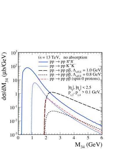
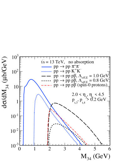
Figure 2: The invariant mass distributions for centrally produced $\pi^{+}\pi^{-}$, $K^{+}K^{-}$ and $p\bar{p}$ systems for different experimental conditions at $\sqrt{s}=13$ TeV. Results for the combined tensor-pomeron and reggeon exchanges and $\Lambda_{off,E}=1$ GeV are presented. For the $p\bar{p}$ production we show results also for $\Lambda_{off,E}=0.8$ GeV; see (14). No absorption effects were included here.

In Fig. 2 we compare the invariant mass distributions for the $\pi^{+}\pi^{-}$, $K^{+}K^{-}$ and $p\bar{p}$ cases for two different experimental conditions at $\sqrt{s}=13$ TeV. In our calculations we have included both pomeron and reggeon exchanges. The distribution in $p\bar{p}$ invariant mass has much larger threshold but is also much less steep, compared to that for production of pseudoscalar meson pairs. This effect is related to the spin of the produced particles (1/2 versus 0). We hope for a confirmation of the slope of the invariant mass distribution, e.g., by the ATLAS or the ALICE collaboration. We see from Fig. 2 that the normalisations of the $M_{34}$ distributions for $p\bar{p}$ are very sensitive to the cutoff parameter $\Lambda_{off,E}$ of (14). In addition, we have the effects of absorption corrections. To fix the magnitudes of these two effects, we will have, at the moment, to have recourse to experimental input which, presumably, will come soon.

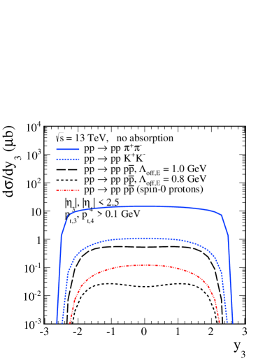
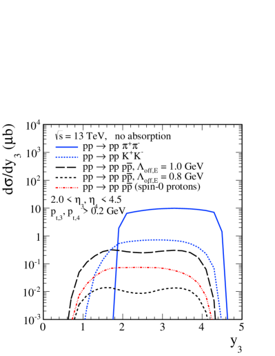
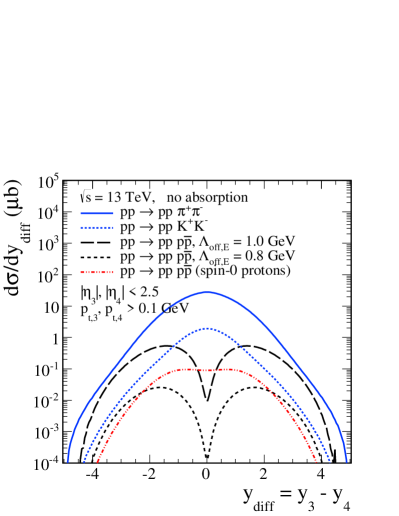
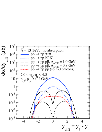
Figure 3: The differential cross sections for various processes at $\sqrt{s}=13$ TeV. In the top panels we show the rapidity distributions obtained for the tensor pomeron and reggeon exchanges. In the bottom panels we show the distributions in the rapidity difference between the centrally produced hadrons. No absorption effects were included here.

In Fig. 3, we show the rapidity distributions (the top panels) and the distributions in rapidity difference ${\rm y}_{diff}={\rm y}_{3}-{\rm y}_{4}$ (the bottom panels) for the ATLAS and LHCb pseudorapidity ranges. The distribution in the (anti)proton rapidity looks rather standard while the distribution for ${\rm y}_{diff}$ is very special. We predict a dip in the rapidity difference between the antiproton and proton for ${\rm y}_{diff}=0$. The dip is caused by a good separation of ${\rm\hat{t}}$ and ${\rm\hat{u}}$ contributions in (${\rm y}_{3},{\rm y}_{4}$) space. This novel effect is inherently related to the spin 1/2 of the produced hadrons. We have checked that for the $p\bar{p}$ production the ${\rm\hat{t}}$- and ${\rm\hat{u}}$-channel diagrams interfere destructively for $(C_{1},C_{2})=(1,1)$ and $(-1,-1)$ exchanges and constructively for $(1,-1)$ and $(-1,1)$ exchanges. For the $\pi^{+}\pi^{-}$ production, we get the opposite interference effects between the ${\rm\hat{t}}$- and ${\rm\hat{u}}$-channel diagrams.

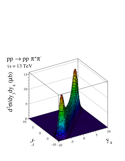
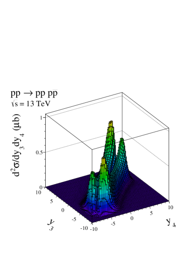
Figure 4: The two-dimensional distributions in (${\rm y}_{3},{\rm y}_{4}$) for two processes at $\sqrt{s}=13$ TeV. Results for the combined tensor-pomeron and reggeon exchanges are presented. We have taken here $\Lambda_{off,E}=1$ GeV; see (14). No absorption effects were included here. The asymmetry in the right panel will be discussed below.

In Fig. 4 we show the two-dimensional distributions in rapidity of the $\pi^{+}$ and $\pi^{-}$ (the left panel) and of the antiproton and proton (the right panel) for the full phase space. In our calculations we have included both pomeron and reggeon exchanges. The reggeon exchange contributions lead to enhancements of the cross section mostly at large rapidities of the centrally produced hadrons. For the production of the dipion continuum, the cross section is concentrated along the diagonal $\rm{y}_{3}=\rm{y}_{4}$. For the production of $p\bar{p}$ pairs, one can observe that the dip extends over the whole diagonal in (${\rm y}_{3},{\rm y}_{4}$) space.

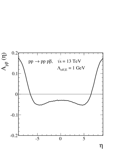
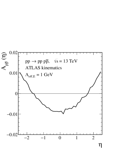
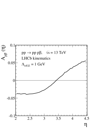
Figure 5: The asymmetry $A_{p\bar{p}}(\eta)$ (22) as function of the pseudorapidity $\eta$ for the full phase space (the top panel) and for the ATLAS and LHCb pseudorapidity ranges (the bottom panels) at $\sqrt{s}=13$ TeV. Cuts on the transverse momenta of the centrally produced nucleons $p_{t,3},p_{t,4}>0.1$ and 0.2 GeV for the ATLAS and LHCb, respectively, have been imposed.

Figure 5 shows the asymmetry

$$A_{p\bar{p}}(\eta)=\frac{\frac{d\sigma}{d\eta_{3}}(\eta)-\frac{d\sigma}{d\eta_{4}}(\eta)}{\frac{d\sigma}{d\eta_{3}}(\eta)+\frac{d\sigma}{d\eta_{4}}(\eta)}\,,$$ (22)

where $\eta_{3}$ and $\eta_{4}$ are the pseudorapidities of the antiproton and proton, respectively, as a function of the pseudorapidity $\eta$ at $\sqrt{s}=13$ TeV. No absorption effects are included here, but they should approximately cancel in the ratio. Sizeable asymmetries are predicted in the full phase space. Much smaller asymmetries are seen for the limited range of pseudorapidities corresponding to the ATLAS, CMS, and ALICE experiments. The effect is better seen for the LHCb experiment, which covers the higher pseudorapidity region relevant for the reggeon exchanges. The asymmetry is caused by the interference of the $(C_{1},C_{2})=(1,1)$ and $(-1,-1)$ exchanges with the $(C_{1},C_{2})=(1,-1)$ and $(-1,1)$ exchanges; see (5) - (8). The former exchanges give an amplitude that is antisymmetric under $p_{3}\leftrightarrow p_{4}$, whereas the latter exchanges give a symmetric amplitude under $p_{3}\leftrightarrow p_{4}$; see (12) and the discussion following it. Thus, the resulting $p\bar{p}$ distribution will not be symmetric under $p_{3}\leftrightarrow p_{4}$. The biggest contributions to the asymmetry come from the interference of the $(\mathbb{P},\mathbb{P})$ term with the $(\mathbb{P},\omega_{\mathbb{R}})$ and $(\omega_{\mathbb{R}},\mathbb{P})$ contributions to the total amplitude. The prediction is that at larger $|\eta|$ more $\bar{p}$ than $p$ should be observed, while at smaller $|\eta|$, the situation is reversed.

More general asymmetries than (22) can be considered and are again due to the interference of the $(C_{1},C_{2})=(1,1)$ and $(-1,-1)$ with the $(C_{1},C_{2})=(1,-1)$ and $(-1,1)$ exchanges. We emphasize that the following discussion holds for both non-resonant and resonant $p\bar{p}$ production. We can, for instance, consider the one-particle distributions for the central $p$ and $\bar{p}$ in the overall c.m. system,

$$\frac{d^{3}\sigma}{d^{3}p_{3}}(\vec{p}_{3})\quad{\rm for\;the\;antiproton}\,,$$

$$\frac{d^{3}\sigma}{d^{3}p_{4}}(\vec{p}_{4})\quad{\rm for\;the\;proton}\,,$$

and the asymmetry

$$A^{(1)}(\vec{p})=\frac{\frac{d^{3}\sigma}{d^{3}p_{3}}(\vec{p})-\frac{d^{3}\sigma}{d^{3}p_{4}}(\vec{p})}{\frac{d^{3}\sigma}{d^{3}p_{3}}(\vec{p})+\frac{d^{3}\sigma}{d^{3}p_{4}}(\vec{p})}\,.$$ (23)

Here, the leading protons $p(\vec{p}_{1})$ and $p(\vec{p}_{2})$ may be integrated over their whole or only a part of their phase space. We can also consider the two-particle cross section for the centrally produced $p$ and $\bar{p}$: $\frac{d^{6}\sigma}{d^{3}p_{3}d^{3}p_{4}}(\vec{p}_{3},\vec{p}_{4})$. A suitable asymmetry there is

$$A^{(2)}(\vec{p},\vec{p}^{\prime})=\frac{\frac{d^{6}\sigma}{d^{3}p_{3}d^{3}p_{4}}(\vec{p},\vec{p}^{\prime})-\frac{d^{6}\sigma}{d^{3}p_{3}d^{3}p_{4}}(\vec{p}^{\prime},\vec{p})}{\frac{d^{6}\sigma}{d^{3}p_{3}d^{3}p_{4}}(\vec{p},\vec{p}^{\prime})+\frac{d^{6}\sigma}{d^{3}p_{3}d^{3}p_{4}}(\vec{p}^{\prime},\vec{p})}\,.$$ (24)

In words, this asymmetry means the following. We choose two momenta $\vec{p}$ and $\vec{p}^{\prime}$. Then, we ask if the situations ($\bar{p}(\vec{p}),p(\vec{p}^{\prime})$) and ($\bar{p}(\vec{p}^{\prime}),p(\vec{p})$) occur at the same or at a different rate.

Another asymmetry of this type can be constructed from the pseudorapidity distributions $\frac{d^{2}\sigma}{d\eta_{3}d\eta_{4}}(\eta_{3},\eta_{4})$. For two pseudorapidities $\eta$ and $\eta^{\prime}$, we define

$$\widetilde{A}^{(2)}(\eta,\eta^{\prime})=\frac{\frac{d^{2}\sigma}{d\eta_{3}d\eta_{4}}(\eta,\eta^{\prime})-\frac{d^{2}\sigma}{d\eta_{3}d\eta_{4}}(\eta^{\prime},\eta)}{\frac{d^{2}\sigma}{d\eta_{3}d\eta_{4}}(\eta,\eta^{\prime})+\frac{d^{2}\sigma}{d\eta_{3}d\eta_{4}}(\eta^{\prime},\eta)}\,.$$ (25)

For the quantity $\frac{d^{2}\sigma}{d\eta_{3}d\eta_{4}}(\eta_{3},\eta_{4})$ and the asymmetry $\widetilde{A}^{(2)}(\eta,\eta^{\prime})$, we have also investigated effects of an odderon using the parameters of (39) - (41). In Fig. 6, we show, in two-dimensional plots, the ratios

$$R^{(\mathbb{P}+\mathbb{R})}(\eta_{3},\eta_{4})=\frac{d^{2}\sigma^{(\mathbb{P}+\mathbb{R})}/d\eta_{3}d\eta_{4}}{d^{2}\sigma^{(\mathbb{P})}/d\eta_{3}d\eta_{4}}\,,$$ (26)

$$R^{(\mathbb{P}+\mathbb{R}+\mathbb{O})}(\eta_{3},\eta_{4})=\frac{d^{2}\sigma^{(\mathbb{P}+\mathbb{R}+\mathbb{O})}/d\eta_{3}d\eta_{4}}{d^{2}\sigma^{(\mathbb{P}+\mathbb{R})}/d\eta_{3}d\eta_{4}}$$ (27)

for $\sqrt{s}=13$ TeV and $-6\leqslant\eta_{3},\eta_{4}\leqslant 6$. We see that in the limited range of pseudorapidities corresponding to the ATLAS and LHCb experiments the effects of the secondary reggeons are predicted to be in the ranges of 2 - 11 % and 5 - 26 %, respectively. The addition of an odderon with the parameters of (41) has only an effect of less than 0.5 %.

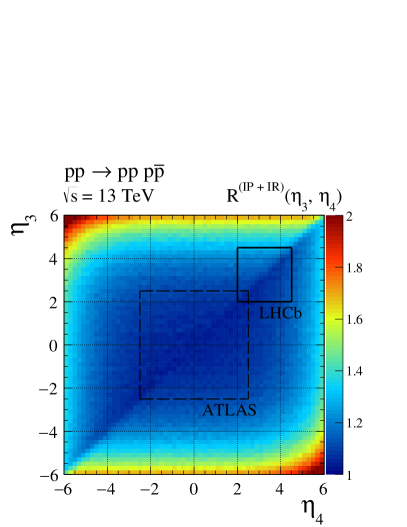
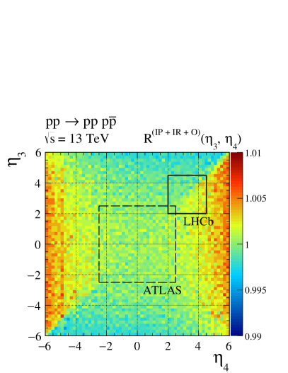
Figure 6: The ratios $R(\eta_{3},\eta_{4})$ at $\sqrt{s}=13$ TeV and $p_{t,3},p_{t,4}>0.2$ GeV. The left panel represents the result for the ratio $R^{(\mathbb{P}+\mathbb{R})}(\eta_{3},\eta_{4})$ (26). The right panel shows the result for $R^{(\mathbb{P}+\mathbb{R}+\mathbb{O})}(\eta_{3},\eta_{4})$ (27). Note that different z scales are taken for the left and right panels. Calculations were done with the parameters of Appendix A. In addition regions of the coverage for the ATLAS and LHCb experiments are shown.

In Fig. 7 we show the asymmetry (25) including pomeron and reggeon exchanges. For the investigated pseudorapidity range the asymmetries due to pomeron plus reggeon exchange show a characteristic pattern: positive for $|\eta|>|\eta^{\prime}|$ and negative for $|\eta|<|\eta^{\prime}|$. That is, antiprotons are predicted to come out typically with a higher absolute value of the (pseudo)rapidity than protons. In Fig. 7 the inclusion of the odderon would hardly change the result, only at the level of less than 1 %. This is less than theoretical uncertainties associated with the reggeon exchanges.

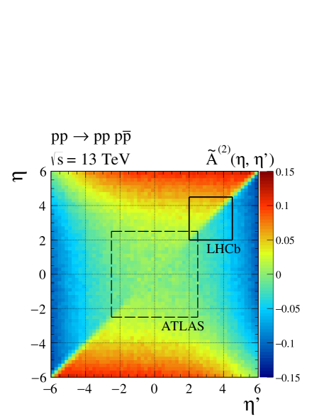
Figure 7: The asymmetry $\widetilde{A}^{(2)}(\eta,\eta^{\prime})$ (25) at $\sqrt{s}=13$ TeV and $p_{t,3},p_{t,4}>0.2$ GeV. Shown is the result including pomeron and reggeon exchanges.

Finally, we note that for calculations of the asymmetries (22) - (25) it is essential to use a model in which the pomeron is correctly treated as a $C=+1$ exchange, as is the case for our tensor pomeron. On the other hand, in a vector-pomeron model, using standard QFT rules for the vertices, we will have effectively a $C=-1$ pomeron. Then, all exchanges will be, effectively, $(C_{1},C_{2})=(-1,-1)$ and all asymmetries (22) to (25) will be zero. We cannot and do not exclude the possibility that by introducing some ad hoc sign changes in amplitudes one can generate non-zero asymmetries also in vector-pomeron models. But we emphasize that in the tensor-pomeron model Ewerz:2013kda asymmetries are generated in a natural and straightforward way. Thus, experimental observations of such asymmetries would give strong support for the tensor-pomeron concept.

Now, we turn to $p\bar{p}$ production via resonances. Not much is known about mesonic resonances in the $p\bar{p}$ channel, especially for those produced in the diffractive processes. Exceptions may be production of $\eta_{c}$ and $\chi_{c}$ mesons for which the branching fractions to the $p\bar{p}$ channel are relatively well known Olive:2016xmw . There is also some evidence for the presence of the $f_{2}(1950)$ resonance in the $\gamma\gamma\to p\bar{p}$ reaction Klusek-Gawenda:2017lgt . Although statistics of the ISR data Akesson:1985rn ; Breakstone:1989ty was poor for the $pp\to ppp\bar{p}$ reaction, the data show a large low-mass enhancement. With good statistics one could study at the LHC the distribution $d^{2}\sigma/dM_{34}d{\rm y}_{diff}$ for the $pp\to ppp\bar{p}$ reaction. In the right panel of Fig. 8, we show this distribution for the non-resonant $p\bar{p}$ production. For comparison, in the left panel of Fig. 8, the distribution for the $pp\to pp\pi^{+}\pi^{-}$ reaction is shown. For $p\bar{p}$ production one can observe a characteristic ridge at the edge of the $(M_{34},{\rm y}_{diff})$ space. The interior is then free of the diffractive continuum. There, the identification of possible resonances should be easier. In reality, the presence of resonances may destroy the dip as resonances are expected to give a dominant contribution just at ${\rm y}_{diff}=0$.

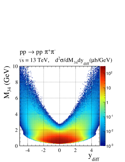
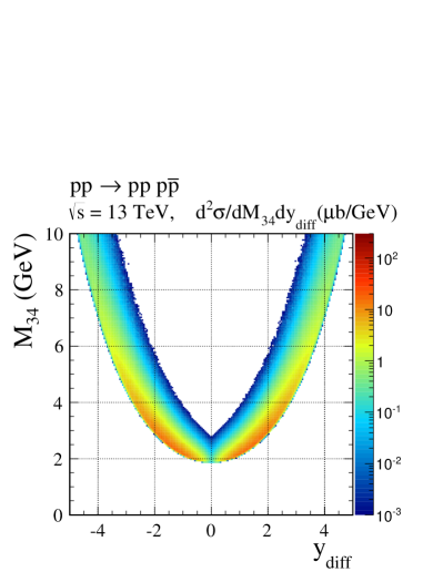
Figure 8: The two-dimensional distributions in ($M_{34},\rm{y}_{diff}$) for the diffractive continuum $\pi^{+}\pi^{-}$ (the left panel) and $p\bar{p}$ (the right panel) production for the full phase space at $\sqrt{s}=13$ TeV. Results for the combined tensor-pomeron and reggeon exchanges are shown. We have taken here $\Lambda_{off,E}=1$ GeV. No absorption effects have been included here.

In Fig. 9, we discuss one possible scenario for the $pp\to ppp\bar{p}$ reaction. We take into account the non-resonant continuum including both pomeron and reggeon exchanges and, as an example, the scalar $f_{0}(2100)$ resonance created by the pomeron-pomeron fusion. The scalar $f_{0}(2100)$ was observed in $p\bar{p}$ annihilation into the $\eta\eta$ channel using a partial wave analysis of Crystal Barrel data Anisovich:2011bw ; Anisovich:2000af . It may be considered as a second scalar glueball, probably mixed with $q\bar{q}$ states. For the continuum term, we take $\Lambda_{off,E}=0.8$ GeV in (14), while for the resonant term we take $\Lambda_{f_{0}}=1$ GeV in (18) and $g_{\mathbb{P}\mathbb{P}f_{0}}^{\prime}\,g_{f_{0}p\bar{p}}=0.8$, $g_{\mathbb{P}\mathbb{P}f_{0}}^{\prime\prime}=0$; see (16) and Appendix A of Lebiedowicz:2013ika . Here, the coupling constants are fixed arbitrarily. We only want to give an example for the effects to be expected from resonance contributions. We show the distributions in the $p\bar{p}$ invariant mass (the left panel) and in ${\rm y}_{diff}$ (the right panel) at $\sqrt{s}=13$ TeV. Clearly, the resonant contribution leads to enhancements at low $M_{p\bar{p}}$ and in the central region of ${\rm y}_{diff}$. We can see that the complete result indicates an interference effect of the continuum and $f_{0}(2100)$ terms. With the parameters used here we get for the complete cross section 113 nb for the ATLAS cuts ($|\eta_{3}|,|\eta_{4}|<2.5$, $p_{t,3},p_{t,4}>0.1$ GeV) and 35 nb for the LHCb cuts ($2<\eta_{3},\eta_{4}<4.5$, $p_{t,3},p_{t,4}>0.2$ GeV) on centrally produced $p\bar{p}$. Here the absorption effects are not included. It is worth adding that the cross section for the resonant contribution is concentrated along the diagonal ${\rm y}_{3}\simeq{\rm y}_{4}$ in (${\rm y}_{3},{\rm y}_{4}$) space, exactly in the valley of the continuum contribution (see the right panel in Fig. 4).

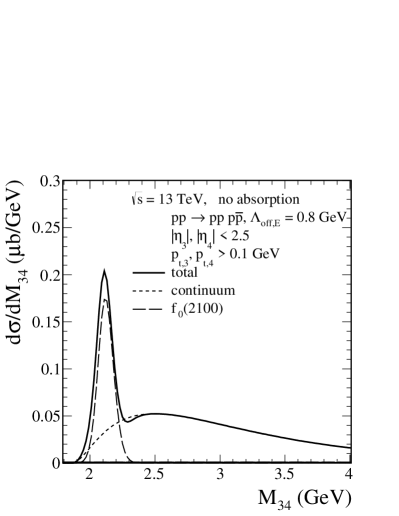
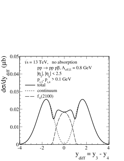
Figure 9: The differential cross sections for $pp\to ppp\bar{p}$ at $\sqrt{s}=13$ TeV for continuum plus $f_{0}(2100)$ production. The distributions in the $p\bar{p}$ invariant mass (the left panel) and in ${\rm y}_{diff}$ (the right panel) are shown. No absorption effects were included here.

In Fig. 10 we show two-dimensional distribution in $(M_{34},{\rm y}_{diff})$ for $pp\to ppp\bar{p}$ obtained from the non-resonant plus the $f_{0}(2100)$ resonant contributions. Here, the model parameters were chosen as in Fig. 9. Comparing with the right panel of Fig. 8 we see clearly that the resonance contribution is centered around $M_{34}=2.1$ GeV and is approximately uniform in ${\rm y}_{diff}$ for $|{\rm y}_{diff}|\lesssim 1$. Note that for $M_{34}\to 2m_{p}$, that is, for $\vec{p}_{3}-\vec{p}_{4}\to 0$ both, the dominant $(\mathbb{P},\mathbb{P})$ continuum contribution, as well as the $f_{0}(2100)$ resonance contribution must vanish; see (12). This is clearly seen in Fig. 10.

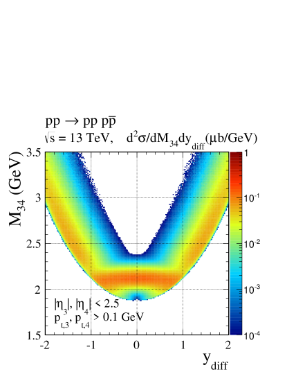
Figure 10: The two-dimensional distribution in ($M_{34},\rm{y}_{diff}$) for the $p\bar{p}$ production at $\sqrt{s}=13$ TeV including the continuum and the $f_{0}(2100)$ contribution. The strength of the resonance contribution is chosen arbitrarily. No absorption effects were included here.

Also, azimuthal correlations are interesting for central exclusive $p\bar{p}$ production. From the experimental point of view, this typically would require that the momenta of the leading protons are measured. Then, one could study, for instance, the distributions in the angle $\phi_{12}$ between the transverse momenta $\vec{p}_{t,1}$ and $\vec{p}_{t,2}$ of the leading protons. For low-energy central-meson production these angular distributions have been extensively discussed in Barberis:1996iq ; Barberis:1997ve ; Barberis:1998ax ; Barberis:1998sr ; Barberis:1999cq ; Barberis:2000em ; Kirk:2000ws , Close:1999is ; Close:1999bi ; Close:2000dx , and from the tensor pomeron point of view in Lebiedowicz:2013ika . Angular distributions for glueball production have been discussed in Iatrakis:2016rvj . Since we have constructed in the present paper a model for central $p\bar{p}$ production at the amplitude level we could also discuss such azimuthal correlations. We have checked that our model, including both the continuum and the scalar resonance $f_{0}(2100)$, taking into account only the $(l,S)=(0,0)$ coupling in (16) gives a rather flat $\phi_{12}$ distribution, unlike for central $\pi^{+}\pi^{-}$ production Lebiedowicz:2014bea ; Lebiedowicz:2016ioh . This is consistent with a measurement made by the WA102 Collaboration; see Fig. 4 (a) of Barberis:1998sr . But since present LHC experiments are not yet equipped for such measurements, we leave this for a further publication.

V Conclusions

In the present article, we have discussed exclusive production of $p\bar{p}$ and $\Lambda\overline{\Lambda}$ pairs in proton-proton collisions. At the present stage, we have taken into account mainly the diffractive production of the $p\bar{p}$ continuum. The amplitudes have been calculated using Feynman rules within the tensor-pomeron model Ewerz:2013kda and taking into account the spins of the produced particles. Applying this model to our reactions here we had to introduce some form factors containing suitable cut-off parameters; see (14) and (18). A first estimate of these cut-off parameters was made by comparing to low-statistics ISR data in which mostly the integrated cross section for $pp\to ppp\bar{p}$ was measured at $\sqrt{s}=62$ GeV. There, we need a cut-off parameter $\Lambda_{off,E}\sim 1$ GeV in (14). The form factors and corresponding cut-off parameters needed to describe the off-shellness of the intermediate $t$-/$u$-channel protons are not well known and have to be fitted in the future to experimental data. They influence mostly the absolute normalization of the cross sections and have almost no influence on shapes of distributions. In this paper we did not concentrate on the absolute normalization but rather on relative effects by studying the qualitative features of the $pp\to ppp\bar{p}$ reaction in the tensor-pomeron model. To describe the relatively low-energy ISR and WA102 experiments, we find that we have to include also subleading reggeon exchanges in addition to the two-pomeron exchange.

For our predictions for the LHC we have used the off-shell proton form factor parameter in (14), $\Lambda_{off,E}$, in the range between 0.8 and 1 GeV. The invariant mass distribution for $p\bar{p}$ pairs is predicted to extend to larger dihadron invariant masses than for the production of $\pi^{+}\pi^{-}$ or $K^{+}K^{-}$ or artificial pseudoscalar nucleons. This is strongly related to spin 1/2 for nucleons versus spin 0 for pseudoscalar mesons.

Especially interesting is the distribution in the rapidity difference between antiproton and proton. For continuum $p\bar{p}$ production, we predict a dip at ${\rm y}_{diff}=0$, in contrast to $\pi^{+}\pi^{-}$ and $K^{+}K^{-}$ production in which a maximum of the cross section occurs at ${\rm y}_{diff}=0$. The dip is caused by a good separation of ${\rm\hat{t}}$ and ${\rm\hat{u}}$ contributions in (${\rm y}_{3},{\rm y}_{4}$) space and destructive interference of them along the diagonal $\rm{y}_{3}=\rm{y}_{4}$ characteristic for our Feynman diagrammatic calculation with correct treatment of spins.

In our calculations, we have included both pomeron and reggeon exchanges. The reggeon exchange contributions lead to enhancements at large absolute values of the $p$ and $\bar{p}$ (pseudo)rapidities. A similar effect was predicted for the $pp\to pp\pi^{+}\pi^{-}$ reaction in Lebiedowicz:2010yb . We have predicted asymmetries in the (pseudo)rapidity distributions of the centrally produced antiproton and proton. The asymmetry is caused by interference effects of the dominant $(\mathbb{P},\mathbb{P})$ with the subdominant $(\mathbb{R}_{-},\mathbb{P}+\mathbb{R}_{+})$ and $(\mathbb{P}+\mathbb{R}_{+},\mathbb{R}_{-})$ exchanges. It should be emphasized that limited detector acceptances in experimental searches at the LHC might affect the size of the asymmetry. The asymmetry should be much more visible for the LHCb experiment which covers a region of larger pseudorapidities where the reggeon exchanges become more relevant. Also the odderon will contribute to such asymmetries. However, we find for typical odderon parameters allowed by recent $pp$ elastic data Antchev:2017yns only very small effects, roughly a factor 10 smaller than the effects due to reggeons as predicted in the present paper.

All our predictions here have been done for the tensor-pomeron model. In the literature, often, a vector pomeron is used, which is – strictly speaking – inconsistent with the rules of quantum field theory as it gives the pomeron charge conjugation $C=-1$ instead of $C=+1$. This is discussed, e.g., in Refs. Ewerz:2013kda ; Lebiedowicz:2016ioh ; Ewerz:2016onn . Although the vector-pomeron model is incorrect from the field theory point of view, it leads to almost the same distributions including the prediction of the dip at ${\rm y}_{diff}=0$. This is not too surprising since the leading $(\mathbb{P},\mathbb{P})$ fusion term has $(C_{1},C_{2})=(1,1)$ for the tensor pomeron and $(C_{1},C_{2})=(-1,-1)$ for the vector pomeron, giving in both cases a state with $C=+1$. The situation is quite different for pomeron-reggeon, $(\mathbb{P},\mathbb{R}_{-})$ and $(\mathbb{R}_{-},\mathbb{P})$, exchange. There, we get with a tensor pomeron a $C=-1$ state, with a vector pomeron again a $C=+1$ state. The interference of $p\bar{p}$ amplitudes with $C=+1$ and $C=-1$ leads to the asymmetries discussed in Sec. IV. We see great difficulties producing such asymmetries in a vector-pomeron model in which only $C=+1$ $p\bar{p}$ amplitudes occur. Therefore, we find it an important task for experimentalist to study the asymmetries (22) - (25). If non-zero asymmetries are found we would have a further strong argument in favour of the tensor-pomeron concept.

In the present study, we have focused mainly on the production of continuum $p\bar{p}$ pairs in the framework of the tensor-pomeron model treating correctly the spin degrees of freedom. Not much is known about diffractively produced $p\bar{p}$ resonances. Any experimentally observed distortions from our continuum-$p\bar{p}$ predictions may therefore signal the presence of resonances. This could give new interesting information for meson spectroscopy. We have discussed a first qualitative attempt to “reproduce” the experimentally observed behaviors of the $p\bar{p}$ invariant mass ($M_{34}$) spectra observed in Akesson:1985rn ; Breakstone:1989ty ; Barberis:1998sr . Our calculation shows that the diffractive production of $p\bar{p}$ through the $s$-channel $f_{0}(2100)$ resonance leads to an enhancement at low $M_{34}$ and that the resonance contribution is concentrated at $|{\rm y}_{diff}|<1$. In general, more resonances can contribute, e.g., $f_{0}(2020)$, $f_{0}(2200)$, and $f_{0}(2300)$. Contributions of other states, such as $f_{2}(1950)$, are not excluded. Also, the subthreshold $m_{R}<2m_{p}$ resonances that would effectively generate a continuum $p\bar{p}$ contribution should be taken into account; see Klusek-Gawenda:2017lgt . Interference effects between the continuum and resonant mechanisms certainly will occur; see Fig. 9.

The predictions made for $p\bar{p}$ production can be easily repeated for diffractive $\Lambda\overline{\Lambda}$ pair production. Here, the uncertainties for the continuum contribution are slightly larger than for the $p\bar{p}$ production (higher off-shell effects and less-known interaction parameters). However, here, the resonance contributions are expected to be much smaller if present at all. Any clear observation of a resonance in the $\Lambda\overline{\Lambda}$ channel would, therefore, be a sensation, and the result would definitely go to the Particle Data Book. On the other hand, a lack of such resonances would allow a verification of the minimum at ${\rm y}_{diff}=0$, which we predict using the correct treatment of the spin degrees of freedom in the Regge-like calculations of central exclusive baryon-antibaryon production.

Appendix A Effective propagators and vertices for pomeron, reggeon, and odderon exchange

Here, we collect the expressions for our effective exchanges and vertex functions as given in Sec. 3 of Ewerz:2013kda in order to make our present paper self-contained. For extensive discussions motivating the following expressions, we refer to Ewerz:2013kda .

Our effective pomeron propagator reads

$$i\Delta^{(\mathbb{P})}_{\mu\nu,\kappa\lambda}(s,t)=\frac{1}{4s}\left(g_{\mu\kappa}g_{\nu\lambda}+g_{\mu\lambda}g_{\nu\kappa}-\frac{1}{2}g_{\mu\nu}g_{\kappa\lambda}\right)(-is\alpha^{\prime}_{\mathbb{P}})^{\alpha_{\mathbb{P}}(t)-1}$$ (28)

and fulfills the following relations:

$$\begin{split}&\Delta^{(\mathbb{P})}_{\mu\nu,\kappa\lambda}(s,t)=\Delta^{(\mathbb{P})}_{\nu\mu,\kappa\lambda}(s,t)=\Delta^{(\mathbb{P})}_{\mu\nu,\lambda\kappa}(s,t)=\Delta^{(\mathbb{P})}_{\kappa\lambda,\mu\nu}(s,t)\,,\\ &g^{\mu\nu}\Delta^{(\mathbb{P})}_{\mu\nu,\kappa\lambda}(s,t)=0,\quad g^{\kappa\lambda}\Delta^{(\mathbb{P})}_{\mu\nu,\kappa\lambda}(s,t)=0\,.\end{split}$$ (29)

Here, the pomeron trajectory $\alpha_{\mathbb{P}}(t)$ is assumed to be of standard linear form, see e.g. Donnachie:2002en ,

$$\alpha_{\mathbb{P}}(t)=\alpha_{\mathbb{P}}(0)+\alpha^{\prime}_{\mathbb{P}}\,t\,,$$

$$\alpha_{\mathbb{P}}(0)=1.0808\,,$$

$$\alpha^{\prime}_{\mathbb{P}}=0.25\;\mathrm{GeV}^{-2}\,.$$ (30)

The pomeron-proton vertex function, supplemented by a vertex form factor, taken here to be the Dirac electromagnetic form factor of the proton for simplicity, has the form

$$i\Gamma_{\mu\nu}^{(\mathbb{P}pp)}(p^{\prime},p)=i\Gamma_{\mu\nu}^{(\mathbb{P}\bar{p}\bar{p})}(p^{\prime},p)$$

$$\quad=-i3\beta_{\mathbb{P}NN}F_{1}\bigl{(}(p^{\prime}-p)^{2}\bigr{)}\left\{\frac{1}{2}\left[\gamma_{\mu}(p^{\prime}+p)_{\nu}+\gamma_{\nu}(p^{\prime}+p)_{\mu}\right]-\frac{1}{4}g_{\mu\nu}(p\!\!\!/^{\prime}+p\!\!\!/)\right\}\,,\qquad$$ (31)

with $\beta_{\mathbb{P}NN}=1.87$ GeV^-1.

The ansatz for the $C=+1$ reggeons $\mathbb{R}_{+}=f_{2\mathbb{R}},a_{2\mathbb{R}}$ is similar to (28) - (31). The $\mathbb{R}_{+}$ propagator is obtained from (28) with the replacements

$$\alpha_{\mathbb{P}}(t)\to\alpha_{\mathbb{R}_{+}}(t)=\alpha_{\mathbb{R}_{+}}(0)+\alpha^{\prime}_{\mathbb{R}_{+}}\,t\,,$$

$$\alpha_{\mathbb{R}_{+}}(0)=0.5475\,,$$

$$\alpha^{\prime}_{\mathbb{R}_{+}}=0.9\;\mathrm{GeV}^{-2}\,.$$ (32)

The $f_{2\mathbb{R}}$- and $a_{2\mathbb{R}}$-proton vertex functions are obtained from (31) with the replacements ($M_{0}=1$ GeV)

$$3\beta_{\mathbb{P}NN}\to\frac{g_{f_{2\mathbb{R}}pp}}{M_{0}}\,,$$

$$g_{f_{2\mathbb{R}}pp}=11.04\,,$$ (33)

and

$$3\beta_{\mathbb{P}NN}\to\frac{g_{a_{2\mathbb{R}}pp}}{M_{0}}\,,$$

$$g_{a_{2\mathbb{R}}pp}=1.68\,,$$ (34)

respectively.

Our ansatz for the $C=-1$ reggeons $\mathbb{R}_{-}=\omega_{\mathbb{R}},\rho_{\mathbb{R}}$ reads as follows. We assume an effective vector propagator

$$i\Delta^{(\mathbb{R}_{-})}_{\mu\nu}(s,t)=ig_{\mu\nu}\frac{1}{M_{-}^{2}}(-is\alpha^{\prime}_{\mathbb{R}_{-}})^{\alpha_{\mathbb{R}_{-}}(t)-1}\,,$$ (35)

with

$$\alpha_{\mathbb{R}_{-}}(t)=\alpha_{\mathbb{R}_{-}}(0)+\alpha^{\prime}_{\mathbb{R}_{-}}\,t\,,$$

$$\alpha_{\mathbb{R}_{-}}(0)=0.5475\,,$$

$$\alpha^{\prime}_{\mathbb{R}_{-}}=0.9\;\mathrm{GeV}^{-2}\,,$$

$$M_{-}=1.41\;\mathrm{GeV}\,.$$ (36)

The $\mathbb{R}_{-}$-proton vertex reads ($\mathbb{R}_{-}=\omega_{\mathbb{R}},\rho_{\mathbb{R}}$)

$$i\Gamma_{\mu}^{(\mathbb{R}_{-}pp)}(p^{\prime},p)=-i\Gamma_{\mu}^{(\mathbb{R}_{-}\bar{p}\bar{p})}(p^{\prime},p)=-ig_{\mathbb{R}_{-}pp}F_{1}\bigl{(}(p^{\prime}-p)^{2}\bigr{)}\gamma_{\mu}\,,$$ (37)

with

$$g_{\omega_{\mathbb{R}}pp}=8.65\,,$$

$$g_{\rho_{\mathbb{R}}pp}=2.02\,.$$ (38)

Our ansatz for the odderon follows (3.16), (3.17) and (3.68), (3.69) of Ewerz:2013kda :

$$i\Delta^{(\mathbb{O})}_{\mu\nu}(s,t)=-ig_{\mu\nu}\frac{\eta_{\mathbb{O}}}{M_{0}^{2}}(-is\alpha^{\prime}_{\mathbb{O}})^{\alpha_{\mathbb{O}}(t)-1}\,,$$ (39)

$$i\Gamma_{\mu}^{(\mathbb{O}pp)}(p^{\prime},p)=-i\Gamma_{\mu}^{(\mathbb{O}\bar{p}\bar{p})}(p^{\prime},p)=-i3\beta_{\mathbb{O}pp}M_{0}\,F_{1}\bigl{(}(p^{\prime}-p)^{2}\bigr{)}\gamma_{\mu}\,.$$ (40)

We take here what we think are representative values for the odderon parameters in light of the recent TOTEM results Antchev:2017yns ,

$$\eta_{\mathbb{O}}=-1\,,$$

$$\alpha_{\mathbb{O}}(t)=\alpha_{\mathbb{O}}(0)+\alpha^{\prime}_{\mathbb{O}}\,t\,,$$

$$\alpha_{\mathbb{O}}(0)=1.05\,,$$

$$\alpha^{\prime}_{\mathbb{O}}=0.25\;\mathrm{GeV}^{-2}\,,$$

$$\beta_{\mathbb{O}NN}=0.2\;\mathrm{GeV}^{-1}\,.$$ (41)

All numbers for the parameters listed above should be considered as default values to be checked and – if necessary – adjusted using relevant experimental data. Some estimates of the present uncertainties of the parameters are discussed in Sec. 3 of Ref. Ewerz:2013kda .

References

- (1) R. Waldi, K. R. Schubert, and K. Winter, Search for glueballs in a pomeron pomeron scattering experiment, Z.Phys. C18 (1983) 301–306.
- (2) T. Åkesson et al., (AFS Collaboration), A search for glueballs and a study of double pomeron exchange at the CERN Intersecting Storage Rings, Nucl.Phys. B264 (1986) 154.
- (3) A. Breakstone et al., (ABCDHW Collaboration), Production of the meson in the Double Pomeron Exchange reaction at GeV, Z.Phys. C31 (1986) 185.
- (4) A. Breakstone et al., (ABCDHW Collaboration), Inclusive Pomeron-Pomeron interactions at the CERN ISR, Z. Phys. C42 (1989) 387. [Erratum: Z. Phys. C43 (1989) 522].
- (5) A. Breakstone et al., (ABCDHW Collaboration), The reaction Pomeron-Pomeron and an unusual production mechanism for the , Z.Phys. C48 (1990) 569–576.
- (6) M. G. Albrow, T. D. Coughlin, and J. R. Forshaw, Central exclusive particle production at high energy hadron colliders, Prog.Part.Nucl.Phys. 65 (2010) 149–184, arXiv:1006.1289 [hep-ph].
- (7) D. Barberis et al., (WA102 Collaboration), A kinematical selection of glueball candidates in central production, Phys.Lett. B397 (1997) 339.
- (8) D. Barberis et al., (WA102 Collaboration), A study of the centrally produced channel in interactions at 450 GeV/, Phys. Lett. B413 (1997) 217–224, arXiv:9707021 [hep-ex].
- (9) D. Barberis et al., (WA102 Collaboration), A study of pseudoscalar states produced centrally in interactions at 450 GeV/, Phys.Lett. B427 (1998) 398, arXiv:9803029 [hep-ex].
- (10) D. Barberis et al., (WA102 Collaboration), A study of the centrally produced baryon - anti-baryon systems in interactions at 450 GeV/, Phys. Lett. B446 (1999) 342–348, arXiv:hep-ex/9812022 [hep-ex].
- (11) D. Barberis et al., (WA102 Collaboration), A coupled channel analysis of the centrally produced and final states in interactions at 450 GeV/, Phys.Lett. B462 (1999) 462–470, arXiv:9907055 [hep-ex].
- (12) D. Barberis et al., (WA102 Collaboration), A study of the , , and observed in the centrally produced final states, Phys.Lett. B474 (2000) 423–426, arXiv:0001017 [hep-ex].
- (13) A. Kirk, Resonance production in central collisions at the CERN Omega Spectrometer, Phys.Lett. B489 (2000) 29, arXiv:0008053 [hep-ph].
- (14) T. A. Aaltonen et al., (CDF Collaboration), Measurement of central exclusive production in collisions at and 1.96 TeV at CDF, Phys. Rev. D91 (2015) 091101, arXiv:1502.01391 [hep-ex].
- (15) V. Khachatryan et al., (CMS Collaboration), Exclusive and semi-exclusive production in proton-proton collisions at = 7 TeV, CMS-FSQ-12-004, CERN-EP-2016-261, arXiv:1706.08310 [hep-ex].
- (16) R. Staszewski, P. Lebiedowicz, M. Trzebiński, J. Chwastowski, and A. Szczurek, Exclusive Production at the LHC with Forward Proton Tagging, Acta Phys.Polon. B42 (2011) 1861–1870, arXiv:1104.3568 [hep-ex].
- (17) L. Adamczyk, W. Guryn, and J. Turnau, Central exclusive production at RHIC, Int.J.Mod.Phys. A29 no. 28, (2014) 1446010, arXiv:1410.5752 [hep-ex].
- (18) R. Sikora, (STAR Collaboration), Central Exclusive Production in the STAR Experiment at RHIC, AIP Conf. Proc. 1819 no. 1, (2017) 040012, arXiv:1611.07823 [nucl-ex].
- (19) J. Pumplin and F. S. Henyey, Double pomeron exchange in the reaction , Nucl.Phys. B117 (1976) 377–396.
- (20) P. Lebiedowicz and A. Szczurek, Exclusive reaction: From the threshold to LHC, Phys.Rev. D81 (2010) 036003, arXiv:0912.0190 [hep-ph].
- (21) P. Lebiedowicz, R. Pasechnik, and A. Szczurek, Measurement of exclusive production of scalar meson in proton-(anti)proton collisions via decay, Phys.Lett. B701 (2011) 434–444, arXiv:1103.5642 [hep-ph].
- (22) P. Lebiedowicz and A. Szczurek, Exclusive reaction at LHC and RHIC, Phys.Rev. D83 (2011) 076002, arXiv:1005.2309 [hep-ph].
- (23) P. Lebiedowicz and A. Szczurek, reaction at high energies, Phys.Rev. D85 (2012) 014026, arXiv:1110.4787 [hep-ph].
- (24) R. Kycia, P. Lebiedowicz, A. Szczurek, and J. Turnau, Triple Regge exchange mechanisms of four-pion continuum production in the reaction, Phys. Rev. D95 no. 9, (2017) 094020, arXiv:1702.07572 [hep-ph].
- (25) L. A. Harland-Lang, V. A. Khoze, and M. G. Ryskin, Modelling exclusive meson pair production at hadron colliders, Eur.Phys.J. C74 (2014) 2848, arXiv:1312.4553 [hep-ph].
- (26) P. Lebiedowicz and A. Szczurek, Revised model of absorption corrections for the process, Phys. Rev. D92 (2015) 054001, arXiv:1504.07560 [hep-ph].
- (27) C. Ewerz, M. Maniatis, and O. Nachtmann, A Model for Soft High-Energy Scattering: Tensor Pomeron and Vector Odderon, Annals Phys. 342 (2014) 31–77, arXiv:1309.3478 [hep-ph].
- (28) C. Ewerz, P. Lebiedowicz, O. Nachtmann, and A. Szczurek, Helicity in Proton-Proton Elastic Scattering and the Spin Structure of the Pomeron, Phys. Lett. B763 (2016) 382–387, arXiv:1606.08067 [hep-ph].
- (29) L. Adamczyk et al., (STAR Collaboration), Single spin asymmetry in polarized proton-proton elastic scattering at GeV, Phys. Lett. B719 (2013) 62, arXiv:1206.1928 [nucl-ex].
- (30) O. Nachtmann, Considerations concerning diffraction scattering in quantum chromodynamics, Annals Phys. 209 (1991) 436.
- (31) S. K. Domokos, J. A. Harvey, and N. Mann, Pomeron contribution to and scattering in AdS/QCD, Phys. Rev. D80 (2009) 126015, arXiv:0907.1084 [hep-ph].
- (32) I. Iatrakis, A. Ramamurti, and E. Shuryak, Pomeron interactions from the Einstein-Hilbert Action, Phys. Rev. D94 no. 4, (2016) 045005, arXiv:1602.05014 [hep-ph].
- (33) P. Lebiedowicz, O. Nachtmann, and A. Szczurek, Exclusive central diffractive production of scalar and pseudoscalar mesons; tensorial vs. vectorial pomeron, Annals Phys. 344 (2014) 301, arXiv:1309.3913 [hep-ph].
- (34) P. Lebiedowicz, O. Nachtmann, and A. Szczurek, and Drell-Söding contributions to central exclusive production of pairs in proton-proton collisions at high energies, Phys. Rev. D91 (2015) 074023, arXiv:1412.3677 [hep-ph].
- (35) A. Bolz, C. Ewerz, M. Maniatis, O. Nachtmann, M. Sauter, and A. Schöning, Photoproduction of pairs in a model with tensor-pomeron and vector-odderon exchange, JHEP 1501 (2015) 151, arXiv:1409.8483 [hep-ph].
- (36) P. Lebiedowicz, O. Nachtmann, and A. Szczurek, Central exclusive diffractive production of the continuum, scalar, and tensor resonances in and scattering within the tensor Pomeron approach, Phys. Rev. D93 (2016) 054015, arXiv:1601.04537 [hep-ph].
- (37) P. Lebiedowicz, O. Nachtmann, and A. Szczurek, Exclusive diffractive production of via the intermediate and states in proton-proton collisions within tensor Pomeron approach, Phys. Rev. D94 no. 3, (2016) 034017, arXiv:1606.05126 [hep-ph].
- (38) P. Lebiedowicz, O. Nachtmann, and A. Szczurek, Central production of in collisions with single proton diffractive dissociation at the LHC, Phys. Rev. D95 no. 3, (2017) 034036, arXiv:1612.06294 [hep-ph].
- (39) M. Kłusek-Gawenda, P. Lebiedowicz, O. Nachtmann, and A. Szczurek, From the reaction to the production of pairs in ultraperipheral ultrarelativistic heavy-ion collisions at the LHC, Phys. Rev. D96 no. 9, (2017) 094029, arXiv:1708.09836 [hep-ph].
- (40) C. C. Kuo et al., (Belle Collaboration), Measurement of production at Belle, Phys. Lett. B621 (2005) 41–55, arXiv:hep-ex/0503006 [hep-ex].
- (41) L. Łukaszuk and B. Nicolescu, A Possible interpretation of rising total cross-sections, Lett. Nuovo Cim. 8 (1973) 405.
- (42) D. Joynson, E. Leader, B. Nicolescu, and C. Lopez, Non-regge and hyper-regge effects in pion-nucleon charge exchange scattering at high energies, Nuovo Cim. A30 (1975) 345.
- (43) C. Ewerz, The Odderon in Quantum Chromodynamics, arXiv:hep-ph/0306137 [hep-ph].
- (44) G. Antchev et al., (TOTEM Collaboration), First determination of the parameter at TeV - probing the existence of a colourless three-gluon bound state, CERN-EP-2017-335.
- (45) E. Martynov and B. Nicolescu, Did TOTEM experiment discover the Odderon?, Phys. Lett. B778 (2018) 414, arXiv:1711.03288 [hep-ph].
- (46) V. A. Khoze, A. D. Martin, and M. G. Ryskin, Elastic proton-proton scattering at 13 TeV, Phys. Rev. D97 no. 3, (2018) 034019, arXiv:1712.00325 [hep-ph].
- (47) V. A. Khoze, A. D. Martin, and M. G. Ryskin, Black disk, maximal Odderon and unitarity, Phys. Lett. B780 (2018) 352, arXiv:1801.07065 [hep-ph].
- (48) F. E. Low, Model of the bare Pomeron, Phys. Rev. D12 (1975) 163.
- (49) S. Nussinov, Colored-Quark Version of Some Hadronic Puzzles, Phys. Rev. Lett. 34 (1975) 1286.
- (50) E. A. Kuraev, L. N. Lipatov, and V. S. Fadin, The Pomeranchuk Singularity in Nonabelian Gauge Theories, Sov. Phys. JETP 45 (1977) 199. [Zh. Eksp. Teor. Fiz. 72 (1977) 377].
- (51) I. I. Balitsky and L. N. Lipatov, The Pomeranchuk Singularity in Quantum Chromodynamics, Sov. J. Nucl. Phys. 28 (1978) 822. [Yad. Fiz. 28 (1978) 1597].
- (52) R. A. Kycia, J. Chwastowski, R. Staszewski, and J. Turnau, GenEx: A simple generator structure for exclusive processes in high energy collisions, arXiv:1411.6035 [hep-ph].
- (53) C. Patrignani et al., (Particle Data Group), Review of Particle Physics, Chin. Phys. C40 no. 10, (2016) 100001.
- (54) G. Alexander et al., Study of the System in Low-Energy Elastic Scattering, Phys. Rev. 173 (1968) 1452–1460.
- (55) D. Bassano et al., Lambda-Proton Interactions at High Energies, Phys. Rev. 160 no. 5, (1967) 1239.
- (56) J. A. Kadyk et al., interactions in momentum range 300 to 1500 MeV/, Nucl. Phys. B27 (1971) 13–22.
- (57) S. Gjesdal et al., A measurement of the total cross-sections for hyperon interactions on protons and neutrons in the momentum range from 6 GeV/ to 21 GeV/, Phys. Lett. 40B (1972) 152–156.
- (58) A. Donnachie, H. G. Dosch, P. V. Landshoff, and O. Nachtmann, Pomeron physics and QCD, Camb. Monogr. Part. Phys. Nucl. Phys. Cosmol. 19 (2002) 1.
- (59) http://pdg.lbl.gov/2017/hadronic-xsections/hadron.html.
- (60) P. Lebiedowicz, O. Nachtmann, and A. Szczurek, Towards a complete study of central exclusive production of the pairs in proton-proton collisions within the tensor pomeron approach, arXiv:1804.04706 [hep-ph].
- (61) A. V. Anisovich et al., Partial wave analysis of , , and , Nucl. Phys. A662 (2000) 319–343, arXiv:1109.1188 [hep-ex].
- (62) A. V. Anisovich et al., Data on , and from 600 to 1940 MeV/, Nucl. Phys. A662 (2000) 344–361.
- (63) F. E. Close and G. A. Schuler, Central production of mesons: Exotic states versus pomeron structure, Phys.Lett. B458 (1999) 127, arXiv:hep-ph/9902243 [hep-ph].
- (64) F. E. Close and G. A. Schuler, Evidence that the pomeron transforms as a nonconserved vector current, Phys.Lett. B464 (1999) 279, arXiv:hep-ph/9905305 [hep-ph].
- (65) F. E. Close, A. Kirk, and G. A. Schuler, Dynamics of glueball and production in the central region of collisions, Phys.Lett. B477 (2000) 13, arXiv:hep-ph/0001158 [hep-ph].