Almost Every Simply Typed $\lambda$-Term
Has a Long $\beta$-Reduction Sequence

Abstract.

It is well known that the length of a $\beta$-reduction sequence of a simply typed $\lambda$-term of order $k$ can be huge; it is as large as $k$-fold exponential in the size of the $\lambda$-term in the worst case. We consider the following relevant question about quantitative properties, instead of the worst case: how many simply typed $\lambda$-terms have very long reduction sequences? We provide a partial answer to this question, by showing that asymptotically almost every simply typed $\lambda$-term of order $k$ has a reduction sequence as long as $(k-1)$-fold exponential in the term size, under the assumption that the arity of functions and the number of variables that may occur in every subterm are bounded above by a constant. To prove it, we have extended the infinite monkey theorem for words to a parameterized one for regular tree languages, which may be of independent interest. The work has been motivated by quantitative analysis of the complexity of higher-order model checking.

1. Introduction

It is well known that a $\beta$-reduction sequence of a simply typed $\lambda$-term can be extremely long. Beckmann [1] showed that, for any $k\geq 0$,

$$\max\{\beta(t)\mid t\text{ is a simply typed }\lambda\text{-term of order }k\text{ and size }n\}={\mathbf{exp}_{k}(\Theta(n))}$$

where $\beta(t)$ is the maximum length of the $\beta$-reduction sequences of the term $t$, and ${\mathbf{exp}_{k}(x)}$ is defined by: ${\mathbf{exp}_{0}(x)}\triangleq x$ and ${\mathbf{exp}_{k+1}(x)}\triangleq 2^{{\mathbf{exp}_{k}(x)}}$. Indeed, the following order-$k$ term [1]:

$$(\overline{2}_{k})^{n}\overline{2}_{k-1}\cdots\overline{2}_{2}(\lambda x^{\mathtt{o}}.a\,x\,x){((\lambda x^{\mathtt{o}}.x)c)},$$

where $\overline{2}_{j}$ is the twice function $\lambda f^{\tau^{(j-1)}}.\lambda x^{\tau^{(j-2)}}.f(f\,x)$ (with $\tau^{(j)}$ being the order-$j$ type defined by: $\tau^{(0)}=\mathtt{o}$ and $\tau^{(j)}=\tau^{(j-1)}\to\tau^{(j-1)}$), has a $\beta$-reduction sequence of length ${\mathbf{exp}_{k}(\Omega(n))}$.

Although the worst-case length of the longest $\beta$-reduction sequence is well known as above, much is not known about the average-case length of the longest $\beta$-reduction sequence: how often does one encounter a term having a very long $\beta$-reduction sequence? In other words, suppose we pick a simply-typed $\lambda$-term $t$ of order $k$ and size $n$ randomly; then what is the probability that $t$ has a $\beta$-reduction sequence longer than a certain bound, like ${\mathbf{exp}_{k}(cn)}$ (where $c$ is some constant)? One may expect that, although there exists a term (such as the one above) whose reduction sequence is as long as ${\mathbf{exp}_{k}(\Omega(n))}$, such a term is rarely encountered.

In the present paper, we provide a partial answer to the above question, by showing that almost every simply typed $\lambda$-term of order $k$ has a $\beta$-reduction sequence as long as $(k-1)$-fold exponential in the term size, under a certain assumption. More precisely, we shall show:

$$\lim_{n\rightarrow\infty}\frac{\#\!\left(\{[t]_{\alpha}\in\Lambda_{n}(k,\iota,\xi)\mid\beta(t)\geq{\mathbf{exp}_{k-1}(n^{p})}\}\right)}{\#\!\left(\Lambda_{n}(k,\iota,\xi)\right)}=1$$

for some constant $p>0$, where $\Lambda_{n}(k,\iota,\xi)$ is the set of ($\alpha$-equivalence classes $[-]_{\alpha}$ of) simply-typed $\lambda$-terms such that the term size is $n$, the order is up to $k$, the (internal) arity is up to $\iota\geq k$ and the number of variable names is up to $\xi$ (see the next section for the precise definition).

Related problems have been studied in the context of the quantitative analysis of untyped $\lambda$-terms [2, 3, 4]. For example, David et al. [2] have shown that almost all untyped $\lambda$-terms are strongly normalizing, whereas the result is opposite in the corresponding combinatory logic. A more sophisticated analysis is, however, required in our case, for considering only well-typed terms, and also for reasoning about the length of a reduction sequence instead of a qualitative property like strong normalization.

To prove our main result above, we have extended the infinite monkey theorem (a.k.a. “Borges’s theorem” [5, p.61, Note I.35]) to a parameterized version for regular tree languages. The infinite monkey theorem states that for any word $w$, a sufficiently long word almost surely contains $w$ as a subword (see Section 2 for a more precise statement). Our extended theorem, roughly speaking, states that, for any regular tree grammar $\mathcal{G}$ that satisfies a certain condition and any family $(U_{m})_{m\in{\rm Nature}}$ of trees (or tree contexts) generated by $\mathcal{G}$ such that $|U_{m}|=\mathrm{O}(m)$, a sufficiently large tree $T$ generated by $\mathcal{G}$ almost surely contains $U_{\lceil p\log{|T|}\rceil}$ as a subtree (where $p$ is some positive constant). Our main result is then obtained by preparing a regular tree grammar for simply-typed $\lambda$-terms, and using as $U_{m}$ a term having a very long $\beta$-reduction sequence, like $(\overline{2}_{k})^{m}\overline{2}_{k-1}\cdots\overline{2}_{2}(\lambda x^{\mathtt{o}}.a\,x\,x)((\lambda x^{\mathtt{o}}.x)c)$ given above. The extended infinite monkey theorem mentioned above may be of independent interest and applicable to other problems.

Our work is a part of our long-term project on the quantitative analysis of the complexity of higher-order model checking [6, 7]. The higher-order model checking asks whether the (possibly infinite) tree generated by a ground-type term of the $\lambda$Y-calculus (or, a higher-order recursion scheme) satisfies a given regular property, and it is known that the problem is $k$-EXPTIME complete for order-$k$ terms [7]. Despite the huge worst-case complexity, practical model checkers [8, 9, 10] have been built, which run fast for many typical inputs, and have successfully been applied to automated verification of functional programs [11, 12, 13, 14]. The project aims to provide a theoretical justification for it, by studying how many inputs actually suffer from the worst-case complexity. Since the problem appears to be hard due to recursion, as an intermediate step towards the goal, we aimed to analyze the variant of the problem considered by Terui [15]: given a term of the simply-typed $\lambda$-calculus (without recursion) of type Bool, decide whether it evaluates to true or false (where Booleans are Church-encoded; see [15] for the precise definition). Terui has shown that even for the problem, the complexity is $k$-EXPTIME complete for order-$(2k+2)$ terms. If, contrary to the result of the present paper, the upper-bound of the lengths of $\beta$-reduction sequences were small for almost every term, then we could have concluded that the decision problem above is easily solvable for most of the inputs. The result in the present paper does not necessarily provide a negative answer to the question above, because one need not necessarily apply $\beta$-reductions to solve Terui’s decision problem.

The present work may also shed some light on other problems on typed $\lambda$-calculi with exponential or higher worst-case complexity. For example, despite DEXPTIME-completeness of ML typability [16, 17], it is often said that the exponential behavior is rarely seen in practice. That is, however, based on only empirical studies. A variation of our technique may be used to provide a theoretical justification (or possibly unjustification).

A preliminary version of this article appeared in Proceedings of FoSSaCS 2017 [18]. Compared with the conference version, we have strengthened the main result (from “almost every $\lambda$-term of size $n$ has $\beta$-reduction sequence as long as $\exp_{k-2}(n)$” to “… as long as $\exp_{k-1}(n^{p})$”), and added proofs. We have also generalized the argument in the conference version to formalize the parameterized infinite monkey theorem for regular tree languages.

The rest of this paper is organized as follows. Section 2 states our main result formally. Section 3 proves the extended infinite monkey theorem, and Section 4 proves the main result. Section 5 discusses related work, and Section 6 concludes this article.

2. Main Results

This section states the main results of this article: the result on the quantitative analysis of the length of $\beta$-reduction sequences of simply-typed $\lambda$-terms (Section 2.1) and the parameterized infinite monkey theorem for regular tree grammars (Section 2.2). The latter is used in the proof of the former in Section 4. In the course of giving the main results, we also introduce various notations used in later sections; the notations are summarized in Appendix A. We assume some familiarity with the simply-typed $\lambda$-calculus and regular tree grammars and omit to define some standard concepts (such as $\beta$-reduction); readers who are not familiar with them may wish to consult [19] about the simply-typed $\lambda$-calculus and [20, 21] about regular tree grammars.

For a set $A$, we denote by $\#\!\left(A\right)$ the cardinality of $A$; by abuse of notation, we write $\#\!\left(A\right)=\infty$ to mean that $A$ is infinite. For a sequence $s$, we also denote by $\#\!\left(s\right)$ the length of $s$. For a sequence $s=a_{1}a_{2}\cdots a_{\#\!\left(s\right)}$ and $i\leq\#\!\left(s\right)$, we write $s{\centerdot}i$ for the $i$-th element $a_{i}$. We write $s_{1}\cdot s_{2}$ or just $s_{1}s_{2}$ for the concatenation of two sequences $s_{1}$ and $s_{2}$. We write $\epsilon$ for the empty sequence. We use $\biguplus$ to denote the union of disjoint sets. For a set $I$ and a family of sets $(A_{i})_{i\in I}$, we define $\coprod_{i\in I}A_{i}\triangleq\biguplus_{i\in I}(\{i\}\times A_{i})=\{(i,a)\mid i\in I,a\in A_{i}\}$. For a map $f$, we denote the domain and image of $f$ by $\mathop{\mathrm{Dom}}(f)$ and $\mathrm{Im}\left(f\right)$, respectively. We denote by $\log{x}$ the binary logarithm $\log_{2}{x}$.

2.1. The Main Result on Quantitative Analysis of the Length of $\beta$-Reductions

The set of (simple) types, ranged over by $\tau,\tau_{1},\tau_{2},\ldots$, is defined by the grammar:

$$\tau::=\mathtt{o}\mid\tau_{1}\rightarrow\tau_{2}.$$

Note that the set of types can also be generated by the following grammar:

$$\tau::=\tau_{1}\to\cdots\to\tau_{k}\to\mathtt{o}$$

where $k\geq 0$; we sometimes use the latter grammar for inductive definitions of functions on types. We also use $\sigma$ as a metavariable for types.

Remark 1.

We have only a single base type $\mathtt{o}$ above. The main result (Theorem 2) would not change even if there are multiple base types.

Let $V$ be a countably infinite set, which is ranged over by $x,y,z\,(\text{and }x^{\prime},x_{1},\text{etc.})$. The set of $\lambda$-terms (or terms), ranged over by $t,t_{1},t_{2},\ldots$, is defined by:

$$t::=x\mid\lambda\overline{x}^{\tau}\!.t\mid t_{1}\,t_{2}\qquad\qquad\overline{x}::=x\mid{\ast}.$$

We call elements of $V\cup\{{\ast}\}$ variables, and use meta-variables $\overline{x},\overline{y},\overline{z}\,(\text{and }\overline{x}^{\prime},\overline{x}_{1},\text{etc.})$ for them. We sometimes omit type annotations and just write $\lambda\overline{x}.t$ for $\lambda\overline{x}^{\tau}\!.t$. We call the special variable ${\ast}$ an unused variable, which may be bound by $\lambda$, but must not occur in the body. In our quantitative analysis below, we will count the number of variable names occurring in a term, except ${\ast}$. For example, the term $\lambda x.\lambda y.\lambda z.x$ in the standard syntax can be represented by $\lambda x.\lambda{\ast}.\lambda{\ast}.x$, and the number of used variables in the latter is counted as $1$.

Terms of our syntax can be translated to usual $\lambda$-terms by regarding elements in $V\cup\{{\ast}\}$ as usual variables. Through this identification we define the notions of free variables, closed terms, and $\alpha$-equivalence $\sim_{\alpha}$. The $\alpha$-equivalence class of a term $t$ is written as $[t]_{\alpha}$. In this article, we distinguish between a term and its $\alpha$-equivalence class, and we always use $[-]_{\alpha}$ explicitly. For a term $t$, we write $\mathbf{FV}(t)$ for the set of all the free variables of $t$.

For a term $t$, we define the set $\mathbf{V}(t)$ of variables (except ${\ast}$) in $t$ by:

$$\mathbf{V}(x)\triangleq\{x\}\quad\mathbf{V}(\lambda x^{\tau}\!.t)\triangleq\{x\}\cup\mathbf{V}(t)\quad\mathbf{V}(\lambda{\ast}^{\tau}\!.t)\triangleq\mathbf{V}(t)\quad\mathbf{V}(t_{1}t_{2})\triangleq\mathbf{V}(t_{1})\cup\mathbf{V}(t_{2}).$$

Note that neither $\mathbf{V}(t)$ nor even $\#\!\left(\mathbf{V}(t)\right)$ is preserved by $\alpha$-equivalence. For example, $t=\lambda x.(\lambda y.y)(\lambda z.x)$ and $t^{\prime}=\lambda x.(\lambda x.x)(\lambda{\ast}.x)$ are $\alpha$-equivalent, but $\#\!\left(\mathbf{V}(t)\right)=3$ and $\#\!\left(\mathbf{V}(t^{\prime})\right)=1$. We write $\mathtt{\#vars}{(t)}$ for $\min_{t^{\prime}\in[t]_{\alpha}}\!\!\#\!\left(\mathbf{V}(t^{\prime})\right)$, i.e., the minimum number of variables required to represent an $\alpha$-equivalent term. For example, for $t=\lambda x.(\lambda y.y)(\lambda z.x)$ above, $\mathtt{\#vars}{(t)}=1$, because $t\sim_{\alpha}t^{\prime}$ and $\#\!\left(\mathbf{V}(t^{\prime})\right)=1$.

A type environment $\Gamma$ is a finite set of type bindings of the form $x:\tau$ such that if $(x:\tau),(x:\tau^{\prime})\in\Gamma$ then $\tau=\tau^{\prime}$; sometimes we regard an environment also as a function. When we write $\Gamma_{1}\cup\Gamma_{2}$, we implicitly require that $(x:\tau)\in\Gamma_{1}$ and $(x:\tau^{\prime})\in\Gamma_{2}$ imply $\tau=\tau^{\prime}$, so that $\Gamma_{1}\cup\Gamma_{2}$ is well formed. Note that $({\ast}:\tau)$ cannot belong to a type environment; we do not need any type assumption for ${\ast}$ since it does not occur in terms.

The type judgment relation $\Gamma\vdash t:\tau$ is inductively defined by the following typing rules.

$$\begin{gathered}\frac{}{x:\tau\vdash x:\tau}\qquad\frac{\Gamma_{1}\vdash t_{1}:\sigma{\rightarrow}\tau\qquad\Gamma_{2}\vdash t_{2}:\sigma}{\Gamma_{1}\cup\Gamma_{2}\vdash t_{1}t_{2}:\tau}\\[10.0pt] \frac{\Gamma^{\prime}\vdash t:\tau\qquad\Gamma^{\prime}=\Gamma\text{ or }\Gamma^{\prime}=\Gamma\cup\{\overline{x}:\sigma\}\qquad\overline{x}\notin\mathop{\mathrm{Dom}}(\Gamma)}{\Gamma\vdash\lambda\overline{x}^{\sigma}\!.t:\sigma{\rightarrow}\tau}\end{gathered}$$

The type judgment relation is equivalent to the usual one for the simply-typed $\lambda$-calculus, except that a type environment for a term may contain only variables that occur free in the term (i.e., if $\Gamma\vdash t:\tau$ then $\mathop{\mathrm{Dom}}(\Gamma)=\mathbf{FV}(t)$). Note that if $\Gamma\vdash t:\tau$ is derivable, then the derivation is unique. Below we consider only well-typed $\lambda$-terms, i.e., those that are inhabitants of some typings.

[Size, Order and Internal Arity of a Term] The size of a term $t$, written $|t|$, is defined by:

$$|x|\triangleq 1\;\;\;\;\;\;|\lambda\overline{x}^{\tau}\!.t|\triangleq|t|+1\;\;\;\;\;\;|t_{1}t_{2}|\triangleq|t_{1}|+|t_{2}|+1.$$

The order and internal arity of a type $\tau$, written $\mathtt{ord}(\tau)$ and $\mathtt{iar}(\tau)$ respectively, are defined by:

$$\mathtt{ord}(\tau_{1}\rightarrow\cdots\rightarrow\tau_{n}\rightarrow\mathtt{o})\triangleq\max(\{0\}\cup\{\mathtt{ord}(\tau_{i})+1\mid 1\leq i\leq n\})$$

$$\mathtt{iar}(\tau_{1}\rightarrow\cdots\rightarrow\tau_{n}\rightarrow\mathtt{o})\triangleq\max(\{n\}\cup\{\mathtt{iar}(\tau_{i})\mid 1\leq i\leq n\})$$

where $n\geq 0$. We denote by $\mathrm{Types}(\delta,\iota)$ the set of types $\{\tau\mid\mathtt{ord}(\tau)\leq\delta,\mathtt{iar}(\tau)\leq\iota\}$. For a judgment $\Gamma\vdash t:\tau$, we define the order and internal arity of $\Gamma\vdash t:\tau$, written $\mathtt{ord}(\Gamma\vdash t:\tau)$ and $\mathtt{iar}(\Gamma\vdash t:\tau)$ respectively, by:

$$\mathtt{ord}(\Gamma\vdash t:\tau)\triangleq\max\{\mathtt{ord}(\tau^{\prime})\mid(\Gamma^{\prime}\vdash t^{\prime}:\tau^{\prime})\text{ occurs in }\Delta\}$$

$$\mathtt{iar}(\Gamma\vdash t:\tau)\triangleq\max\{\mathtt{iar}(\tau^{\prime})\mid(\Gamma^{\prime}\vdash t^{\prime}:\tau^{\prime})\text{ occurs in }\Delta\}$$

where $\Delta$ is the (unique) derivation tree for $\Gamma\vdash t:\tau$. Note that the notions of size, order, internal arity, and $\beta(t)$ (the maximum length of $\beta$-reduction sequences of $t$, as defined in Section 1) are well-defined with respect to $\alpha$-equivalence.

Recall the term $\overline{2}_{j}\triangleq\lambda f^{\tau^{(j-1)}}.\lambda x^{\tau^{(j-2)}}.f(f\,x)$ (with $\tau^{(j)}$ being the order-$j$ type defined by: $\tau^{(0)}=\mathtt{o}$ and $\tau^{(j)}=\tau^{(j-1)}\to\tau^{(j-1)}$) in Section 1. For $t=\overline{2}_{3}\,\overline{2}_{2}\,(\lambda x^{\mathtt{o}}.x)\,y$, we have $\mathtt{ord}(y\mathbin{:}\mathtt{o}\vdash t:\mathtt{o})=\mathtt{iar}(y\mathbin{:}\mathtt{o}\vdash t:\mathtt{o})=3$. Note that the derivation for $y\mathbin{:}\mathtt{o}\vdash t:\mathtt{o}$ contains the type judgment $\emptyset\vdash\overline{2}_{3}:\tau^{(3)}$, where $\tau^{(3)}=((\mathtt{o}\to\mathtt{o})\to(\mathtt{o}\to\mathtt{o}))\to(\mathtt{o}\to\mathtt{o})\to\mathtt{o}\to\mathtt{o}$, and $\mathtt{ord}(\tau^{(3)})=\mathtt{iar}(\tau^{(3)})=3$.

We now define the sets of ($\alpha$-equivalence classes of) terms with bounds on the order, the internal arity, and the number of variables. [Terms with Bounds on Types and Variables] Let $\delta,\iota,\xi\geq 0$ and $n\geq 1$ be integers. For each $\Gamma$ and $\tau$, $\Lambda(\langle\Gamma;\tau\rangle,\delta,\iota,\xi)$ and $\Lambda_{n}(\langle\Gamma;\tau\rangle,\delta,\iota,\xi)$ are defined by:

$$\Lambda(\langle\Gamma;\tau\rangle,\delta,\iota,\xi) \triangleq\{[t]_{\alpha}\mid\Gamma\vdash t:\tau,\mathtt{ord}(\Gamma\vdash t:\tau)\leq\delta,\mathtt{iar}(\Gamma\vdash t:\tau)\leq\iota,\mathtt{\#vars}{(t)}\leq\xi\}$$

$$\Lambda_{n}(\langle\Gamma;\tau\rangle,\delta,\iota,\xi) \triangleq\{[t]_{\alpha}\in\Lambda(\langle\Gamma;\tau\rangle,\delta,\iota,\xi)\mid|t|=n\}.$$

We also define:

$${\iota}{\xi}\triangleq\,\biguplus_{\mathclap{\tau\in\mathrm{Types}(\delta,\iota)}}\,\Lambda(\langle\emptyset;\tau\rangle,\delta,\iota,\xi)\qquad\Lambda_{n}(\delta,\iota,\xi)\triangleq\{[t]_{\alpha}\in{\iota}{\xi}\mid|t|=n\}.$$

Intuitively, $\Lambda(\langle\Gamma;\tau\rangle,\delta,\iota,\xi)$ is the set of (the equivalence classes of) terms of type $\tau$ under $\Gamma$, within given bounds $\delta$, $\iota$, and $\xi$ on the order, (internal) arity, and the number of variables respectively; and $\Lambda_{n}(\langle\Gamma;\tau\rangle,\delta,\iota,\xi)$ is the subset of $\Lambda(\langle\Gamma;\tau\rangle,\delta,\iota,\xi)$ consisting of terms of size $n$. The set ${\iota}{\xi}$ consists of (the equivalence classes of) all the closed (well-typed) terms, and $\Lambda_{n}(\delta,\iota,\xi)$ consists of those of size $n$. For example, $t=[\lambda x^{\mathtt{o}}.\lambda y^{\mathtt{o}}.\lambda z^{\mathtt{o}}.x]_{\alpha}$ belongs to $\Lambda_{4}(1,3,1)$; note that $|t|=4$ and $\mathtt{\#vars}{(t)}=\mathtt{\#vars}{(\lambda x^{\mathtt{o}}.\lambda{\ast}.\lambda{\ast}.x)}=1$.

We are now ready to state our main result, which is proved in Section 4.

Theorem 2.

For $\delta,\iota,\xi\geq 2$ and $k=\min\{\delta,\iota\}$, there exists a real number $p>0$ such that

$$\lim_{n\rightarrow\infty}\frac{\#\!\left(\{[t]_{\alpha}\in\Lambda_{n}(\delta,\iota,\xi)\mid\beta(t)\geq{\mathbf{exp}_{k-1}(n^{p})}\}\right)}{\#\!\left(\Lambda_{n}(\delta,\iota,\xi)\right)}=1.$$

As we will see later (in Section 4), the denominator $\#\!\left(\Lambda_{n}(\delta,\iota,\xi)\right)$ is nonzero if $n$ is sufficiently large. The theorem above says that if the order, internal arity, and the number of used variables are bounded independently of term size, most of the simply-typed $\lambda$-terms of size $n$ have a very long $\beta$-reduction sequence, which is as long as $(k-1)$-fold exponential in $n$.

Remark 3.

Recall that, when $k=\delta$, the worst-case length of $\beta$-reduction sequence is $k$-fold exponential [1]. We do not know whether $k-1$ can be replaced with $k$ in the theorem above.

Note that in the above theorem, the order $\delta$, the internal arity $\iota$ and the number $\xi$ of variables are bounded above by a constant, independently of the term size $n$. Our proof of the theorem (given in Section 4) makes use of this assumption to model the set of simply-typed $\lambda$-terms as a regular tree language. It is debatable whether our assumption is reasonable. A slight change of the assumption may change the result, as is the case for strong normalization of untyped $\lambda$-terms [2, 4]. When $\lambda$-terms are viewed as models of functional programs, our rationale behind the assumption is as follows. The assumption that the size of types (hence also the order and the internal arity) is fixed is sometimes assumed in the context of type-based program analysis [22]. The assumption on the number of variables comes from the observation that a large program usually consists of a large number of small functions, and that the number of variables is bounded by the size of each function.

2.2. Regular Tree Grammars and Parameterized Infinite Monkey Theorem

To prove Theorem 2 above, we extend the well-known infinite monkey theorem (a.k.a. “Borges’s theorem” [5, p.61, Note I.35]) to a parameterized version for regular tree grammars, and apply it to the regular tree grammar that generates the set of ($\alpha$-equivalence classes of) simply-typed $\lambda$-terms. Since the extended infinite monkey theorem may be of independent interest, we state it (as Theorem 6) in this section as one of the main results. The theorem is proved in Section 3. We first recall some basic definitions for regular tree grammars in Sections 2.2.1 and 2.2.2, and then state the parameterized infinite monkey theorem in Section 2.2.3.

2.2.1. Trees and Tree Contexts

A ranked alphabet $\Sigma$ is a map from a finite set of terminal symbols to the set of natural numbers. We use the metavariable $a$ for a terminal, and often write $\mathtt{a},\mathtt{b},\mathtt{c},\ldots$ for concrete terminal symbols. For a terminal $a\in\mathop{\mathrm{Dom}}(\Sigma)$, we call $\Sigma(a)$ the rank of $a$. A $\Sigma$-tree is a tree constructed from terminals in $\Sigma$ according to their ranks: $a(T_{1},\ldots,T_{\Sigma(a)})$ is a $\Sigma$-tree if $T_{i}$ is a $\Sigma$-tree for each $i\in\{1,\ldots,\Sigma(a)\}$. Note that $\Sigma(a)$ may be $0$: $a(\,)$ is a $\Sigma$-tree if $\Sigma(a)=0$. We often write just $a$ for $a(\,)$. For example, if $\Sigma=\{\mathtt{a}\mapsto 2,\mathtt{b}\mapsto 1,\mathtt{c}\mapsto 0\}$, then $\mathtt{a}(\mathtt{b}(\mathtt{c}),\mathtt{c})$ is a tree; see (the lefthand side of) Figure 1 for a graphical illustration of the tree. We use the meta-variable $T$ for trees. The size of $T$, written $|T|$, is the number of occurrences of terminals in $T$. We denote the set of all $\Sigma$-trees by ${\mathcal{T}}(\Sigma)$, and the set of all $\Sigma$-trees of size $n$ by ${\mathcal{T}}_{n}(\Sigma)$.

$\Tree[[[].{$\mathtt{c}$}].{$\mathtt{b}$}[].{$\mathtt{c}$}].{$\mathtt{a}$}$

$\Tree[[[].{$[\,]$}[].{$\mathtt{c}$}].{$\mathtt{a}$}[[].{$[\,]$}].{$\mathtt{b}$}].{$\mathtt{a}$}$

Figure 1. A tree $\mathtt{a}(\mathtt{b}(\mathtt{c}),\mathtt{c})$ (left) and a context $\mathtt{a}(\mathtt{a}([\,],\mathtt{c}),\mathtt{b}([\,]))$ (right).

Before introducing grammars, we define tree contexts, which play an important role in our formalization and proof of the (parameterized) infinite monkey theorem for regular tree languages. The set of contexts over a ranked alphabet $\Sigma$, ranged over by $C$, is defined by:

$$C::=[\,]\mid a(C_{1},\ldots,C_{\Sigma(a)}).$$

In other words, a context is a tree where the alphabet is extended with the special nullary symbol $[\,]$. For example, $\mathtt{a}(\mathtt{a}([\,],\mathtt{c}),\mathtt{b}([\,]))$ is a context over $\{\mathtt{a}\mapsto 2,\mathtt{b}\mapsto 1,\mathtt{c}\mapsto 0\}$; see (the righthand side of) Figure 1 for a graphical illustration. We write $\mathcal{C}({\Sigma})$ for the set of contexts over $\Sigma$. For a context $C$, we write $\mathtt{hn}(C)$ for the number of occurrences of $[\,]$ in $C$. We call $C$ a $k$-context if $\mathtt{hn}(C)=k$, and an affine context if $\mathtt{hn}(C)\leq 1$. A 1-context is also called a linear context. We use the metavariable $S$ for linear contexts and $U$ for affine contexts. We write $[\,]_{i}$ for the $i$-th hole occurrence (in the left-to-right order) of $C$.

For contexts $C$, $C_{1},\dots,C_{\mathtt{hn}(C)}$, we write $C[C_{1},\dots,C_{\mathtt{hn}(C)}]$ for the context obtained by replacing each $[\,]_{i}$ in $C$ with $C_{i}$. For example, if $C=\mathtt{a}([\,],\mathtt{a}([\,],[\,]))$, $C_{1}=\mathtt{b}([\,])$, $C_{2}=\mathtt{c}$, and $C_{3}=[\,]$, then $C[C_{1},C_{2},C_{3}]=\mathtt{a}(\mathtt{b}([\,]),\mathtt{a}(\mathtt{c},[\,]))$; see Figure 2 for a graphical illustration. Also, for contexts $C$, $C^{\prime}$ and $i\in\{1,\dots,\mathtt{hn}(C)\}$, we write $C[C^{\prime}]_{i}$ for the context obtained by replacing $[\,]_{i}$ in $C$ with $C^{\prime}$. For example, for $C$ and $C_{1}$ above, $C[C_{1}]_{2}=\mathtt{a}([\,],\mathtt{a}(\mathtt{b}([\,]),[\,]))$.

For contexts $C$ and $C^{\prime}$, we say that $C$ is a subcontext of $C^{\prime}$ and write $C\preceq C^{\prime}$ if there exist $C_{0}$, $C_{1},\ldots,C_{\mathtt{hn}(C)}$, and $1\leq i\leq\mathtt{hn}(C_{0})$ such that $C^{\prime}=C_{0}[C[C_{1},\dots,C_{\mathtt{hn}(C)}]]_{i}$. For example, $C=\mathtt{a}(\mathtt{b}([\,]),[\,])$ is a subcontext of $C^{\prime}=\mathtt{a}([\,],\mathtt{a}(\mathtt{b}([\,]),\mathtt{c}))$, because $C^{\prime}=C_{0}[C[[\,],\mathtt{c}]]_{2}$ for $C_{0}=\mathtt{a}([\,],[\,])$; see also Figure 3 for a graphical illustration. The subcontext relation $\preceq$ may be regarded as a generalization of the subword relation. In fact, a word $w=a_{1}\cdots a_{k}$ can be viewed as a linear context $w^{\sharp}=a_{1}(\cdots(a_{k}[\,])\cdots)$; and if $w$ is a subword of $w^{\prime}$, i.e., if $w^{\prime}=w_{1}ww_{2}$, then $w^{\prime\sharp}=w_{1}^{\sharp}[w^{\sharp}[w_{2}^{\sharp}]]$.

$C:$

$\Tree[[].{$[\,]$}[[].{$[\,]$}[].{$[\,]$}].{$\mathtt{a}$}].{$\mathtt{a}$}$

$C_{1}:$

$\Tree[[].{$[\,]$}].{$\mathtt{b}$}$

$C[C_{1},C_{2},C_{3}]:$

$\Tree[[[].{$[\,]$}].{$\mathtt{b}$}[[].{$\mathtt{c}$}[].{$[\,]$}].{$\mathtt{a}$}].{$\mathtt{a}$}$

Figure 2. Context filling (where $C_{2}=c$ and $C_{3}=[\,]$).

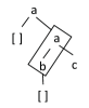
Figure 3. A graphical illustration of a subcontext. The part surrounded by the rectangle is the subcontext $\mathtt{a}(\mathtt{b}([\,]),[\,])$.

The size of a context $U$, written $|U|$, is defined by: $|[\,]|\triangleq 0$ and $|a(C_{1},\dots,C_{\Sigma(a)})|\triangleq 1+|C_{1}|+\dots+|C_{\Sigma(a)}|$. Note that $[\,]$ and 0-ary terminal $a$ have different sizes: $|[\,]|=0$ but $|a|=1$. For a $0$-context $C$, $|C|$ coincides with the size of $C$ as a tree.

2.2.2. Tree Grammars

A regular tree grammar [20, 21] (grammar for short) is a triple ${\mathcal{G}}=(\Sigma,{\mathcal{N}},{\mathcal{R}})$ where (i) $\Sigma$ is a ranked alphabet; (ii) ${\mathcal{N}}$ is a finite set of symbols called nonterminals; (iii) ${\mathcal{R}}$ is a finite set of rewriting rules of the form $N\longrightarrow C[N_{1},\dots,N_{\mathtt{hn}(C)}]$ where $C\in\mathcal{C}({\Sigma})$ and $N,N_{1},\dots,N_{\mathtt{hn}(C)}\in{\mathcal{N}}$. We use the metavariable $N$ for nonterminals. We write $\Sigma\cup{\mathcal{N}}$ for the ranked alphabet $\Sigma\cup\{N\mapsto 0\mid N\in{\mathcal{N}}\}$ and often regard the right-hand-side of a rule as a $(\Sigma\cup{\mathcal{N}})$-tree.

The rewriting relation $\longrightarrow_{\mathcal{G}}$ on ${\mathcal{T}}(\Sigma\cup{\mathcal{N}})$ is inductively defined by the following rules:

$$\frac{(N\longrightarrow C[N_{1},\dots,N_{\mathtt{hn}(C)}])\in{\mathcal{R}}}{N\longrightarrow_{\mathcal{G}}C[N_{1},\dots,N_{\mathtt{hn}(C)}]}\qquad\frac{T_{i}\longrightarrow_{\mathcal{G}}T^{\prime}_{i}}{a(T_{1},\dots,T_{k})\longrightarrow_{\mathcal{G}}a(T_{1},\dots,T_{i-1},T^{\prime}_{i},T_{i+1},\dots,T_{k})}$$

We write $\longrightarrow^{*}_{{\mathcal{G}}}$ for the reflexive and transitive closure of $\longrightarrow_{{\mathcal{G}}}$. For a tree grammar ${\mathcal{G}}=(\Sigma,{\mathcal{N}},{\mathcal{R}})$ and a nonterminal $N\in{\mathcal{N}}$, the language ${\mathcal{L}}\!\left({\mathcal{G}},N\right)$ of $N$ is defined by ${\mathcal{L}}\!\left({\mathcal{G}},N\right)\triangleq\{T\in{\mathcal{T}}(\Sigma)\mid N\longrightarrow^{*}_{\mathcal{G}}T\}$. We also define ${\mathcal{L}}_{n}\!\left({\mathcal{G}},N\right)\triangleq\{T\in{\mathcal{L}}\!\left({\mathcal{G}},N\right)\mid|T|=n\}$. If ${\mathcal{G}}$ is clear from the context, we often omit ${\mathcal{G}}$ and just write $T\longrightarrow^{*}T^{\prime}$, ${\mathcal{L}}\!\left(N\right)$, and ${\mathcal{L}}_{n}\!\left(N\right)$ for $T\longrightarrow^{*}_{\mathcal{G}}T^{\prime}$, ${\mathcal{L}}\!\left({\mathcal{G}},N\right)$, and ${\mathcal{L}}_{n}\!\left({\mathcal{G}},N\right)$, respectively.

We are interested in not only trees, but also contexts generated by a grammar. Let ${\mathcal{G}}=(\Sigma,{\mathcal{N}},{\mathcal{R}})$ be a grammar. The set of context types of ${\mathcal{G}}$, ranged over by $\kappa$, is defined by:

$$\kappa::=N_{1}\cdots N_{k}{\Rightarrow}N$$

where $k\in{\rm Nature}$ and $N,N_{1},\ldots,N_{k}\in{\mathcal{N}}$. Intuitively, $N_{1}\cdots N_{k}{\Rightarrow}N$ denotes the type of $k$-contexts $C$ such that $N\longrightarrow^{*}C[N_{1},\ldots,N_{k}]$. Based on this intuition, we define the sets ${\mathcal{L}}\!\left({\mathcal{G}},\kappa\right)$ and ${\mathcal{L}}_{n}\!\left({\mathcal{G}},\kappa\right)$ of contexts by:

$${\mathcal{L}}\!\left({\mathcal{G}},N_{1}\cdots N_{k}{\Rightarrow}N\right) \triangleq\{C\in\mathcal{C}({\Sigma})\mid\mathtt{hn}(C)=k,N\longrightarrow^{*}_{{\mathcal{G}}}C[N_{1},\ldots,N_{k}]\}$$

$${\mathcal{L}}_{n}\!\left({\mathcal{G}},\kappa\right) \triangleq\{C\in{\mathcal{L}}\!\left({\mathcal{G}},\kappa\right)\mid|C|=n\}.$$

We also write $C\mathbin{:}\kappa$ when $C\in{\mathcal{L}}\!\left({\mathcal{G}},\kappa\right)$ (assuming that ${\mathcal{G}}$ is clear from the context). Note that ${\mathcal{L}}\!\left({\mathcal{G}},{\Rightarrow}N\right)={\mathcal{L}}\!\left({\mathcal{G}},N\right)$, and we identify a context type ${\Rightarrow}N$ with the nonterminal $N$. We call an element in ${\mathcal{L}}\!\left({\mathcal{G}},\kappa\right)$ a $\kappa$-context, and also a $\kappa$-tree if it is a tree. It is clear that, if $C\in{\mathcal{L}}\!\left({\mathcal{G}},N_{1}\cdots N_{k}{\Rightarrow}N\right)$ and $C_{i}\in{\mathcal{L}}\!\left({\mathcal{G}},N^{i}_{1}\cdots N^{i}_{\ell_{i}}{\Rightarrow}N_{i}\right)$ ($i=1,\dots,k$), then $C[C_{1},\dots,C_{k}]\in{\mathcal{L}}\!\left({\mathcal{G}},N^{1}_{1}\cdots N^{1}_{\ell_{1}}\cdots N^{k}_{1}\cdots N^{k}_{\ell_{k}}{\Rightarrow}N\right)$. We also define:

$${\mathcal{L}}\!\left({\mathcal{G}}\right) \triangleq\,\bigcup_{\mathclap{N\in{\mathcal{N}}}}\,{\mathcal{L}}\!\left({\mathcal{G}},N\right) {\mathcal{L}}_{n}\!\left({\mathcal{G}}\right) \triangleq\{T\in{\mathcal{L}}\!\left({\mathcal{G}}\right)\mid|T|=n\}$$

$${\mathcal{S}}({\mathcal{G}}) \triangleq\,\bigcup_{\mathclap{N,N^{\prime}\in{\mathcal{N}}}}\,{\mathcal{L}}\!\left({\mathcal{G}},N{\Rightarrow}N^{\prime}\right) {\mathcal{S}}_{n}({\mathcal{G}}) \triangleq\{S\in{\mathcal{S}}({\mathcal{G}})\mid|S|=n\}$$

$${\mathcal{U}}({\mathcal{G}}) \triangleq{\mathcal{L}}\!\left({\mathcal{G}}\right)\cup{\mathcal{S}}({\mathcal{G}}) {\mathcal{U}}_{n}({\mathcal{G}}) \triangleq\{U\in{\mathcal{U}}({\mathcal{G}})\mid|U|=n\}.$$

Consider the grammar ${\mathcal{G}}_{0}=(\{\mathtt{a}\mapsto 2,\mathtt{b}\mapsto 1,\mathtt{c}\mapsto 0\},\{A_{0},B_{0}\},{\mathcal{R}}_{0})$, where ${\mathcal{R}}_{0}$ consists of:

$$A_{0}\longrightarrow\mathtt{a}(B_{0},B_{0})\qquad A_{0}\longrightarrow\mathtt{c}\qquad B_{0}\longrightarrow\mathtt{b}(A_{0}).$$

Then, $\mathtt{a}([\,],[\,])\in{\mathcal{L}}_{1}\!\left({\mathcal{G}}_{0},B_{0}\,B_{0}{\Rightarrow}A_{0}\right)$ and $\mathtt{a}(\mathtt{b}([\,]),\mathtt{b}(\mathtt{c}))\in{\mathcal{L}}_{4}\!\left({\mathcal{G}}_{0},A_{0}{\Rightarrow}A_{0}\right)$.

This article focuses on grammars that additionally satisfy two properties called strong connectivity and unambiguity. We first define strong connectivity.

[Strong Connectivity [5]] Let ${\mathcal{G}}=(\Sigma,{\mathcal{N}},{\mathcal{R}})$ be a regular tree grammar. We say that $N^{\prime}$ is reachable from $N$ if ${\mathcal{L}}\!\left({\mathcal{G}},N^{\prime}{\Rightarrow}N\right)$ is non-empty, i.e., if there exists a linear context $S\in\mathcal{C}({\Sigma})$ such that $N\longrightarrow^{*}S[N^{\prime}]$. We say that ${\mathcal{G}}$ is strongly connected if for any pair $N,N^{\prime}\in{\mathcal{N}}$ of nonterminals, $N^{\prime}$ is reachable from $N$.

Remark 4.

There is another reasonable, but slightly weaker condition of reachability: $N^{\prime}$ is reachable from $N$ if there exists a $(\Sigma\cup{\mathcal{N}})$-tree $T$ such that $N\longrightarrow^{*}T$ and $N^{\prime}$ occurs in $T$. The two notions coincide if ${\mathcal{L}}\!\left({\mathcal{G}},N\right)\neq\emptyset$ for every $N\in{\mathcal{N}}$. Furthermore this condition can be easily fulfilled by simply removing all the nonterminals $N$ with ${\mathcal{L}}\!\left({\mathcal{G}},N\right)=\emptyset$ and the rules containing those nonterminals.

The grammar ${\mathcal{G}}_{0}$ in Example 2.2.2 is strongly connected, since $\mathtt{b}([\,])\in{\mathcal{L}}\!\left({\mathcal{G}}_{0},A_{0}{\Rightarrow}B_{0}\right)$ and $\mathtt{a}([\,],\mathtt{b}(\mathtt{c}))\in{\mathcal{L}}\!\left({\mathcal{G}}_{0},B_{0}{\Rightarrow}A_{0}\right)$.

Next, consider the grammar ${\mathcal{G}}_{1}=(\{\mathtt{a}\mapsto 2,\mathtt{b}\mapsto 1,\mathtt{c}\mapsto 0\},\{A_{1},B_{1}\},{\mathcal{R}}_{1})$, where ${\mathcal{R}}_{1}$ consists of:

$$A_{1}\longrightarrow\mathtt{a}(\mathtt{c},A_{1})\qquad A_{1}\longrightarrow\mathtt{b}(B_{1})\qquad B_{1}\longrightarrow\mathtt{b}(B_{1})\qquad B_{1}\longrightarrow\mathtt{c}.$$

${\mathcal{G}}_{1}$ is not strongly connected, since ${\mathcal{L}}\!\left({\mathcal{G}}_{1},A_{1}{\Rightarrow}B_{1}\right)=\emptyset$.

To define the unambiguity of a grammar, we define (the standard notion of) leftmost rewriting. The leftmost rewriting relation $\longrightarrow_{{\mathcal{G}},\ell}$ is the restriction of the rewriting relation that allows only the leftmost occurrence of nonterminals to be rewritten. Given $T\in{\mathcal{T}}(\Sigma)$ and $N\in{\mathcal{N}}$, a leftmost rewriting sequence of $T$ from $N$ is a sequence $T_{1},\dots,T_{n}$ of $(\Sigma\cup{\mathcal{N}})$-trees such that

$$N=T_{1}\longrightarrow_{{\mathcal{G}},\ell}T_{2}\longrightarrow_{{\mathcal{G}},\ell}\dots\longrightarrow_{{\mathcal{G}},\ell}T_{n}=T.$$

It is easy to see that $T\in{\mathcal{L}}\!\left({\mathcal{G}},N\right)$ if and only if there exists a leftmost rewriting sequence from $N$ to $T$. [Unambiguity] A grammar ${\mathcal{G}}=(\Sigma,{\mathcal{N}},{\mathcal{R}})$ is unambiguous if, for each $N\in{\mathcal{N}}$ and $T\in{\mathcal{T}}(\Sigma)$, there exists at most one leftmost rewriting sequence from $N$ to $T$.

2.2.3. Parameterized Infinite Monkey Theorem for Tree Grammars

We call a partial function $f$ from ${\rm Nature}$ to with infinite definitional domain (i.e., $\mathop{\mathrm{Dom}}(f)=\{n\in{\rm Nature}\mid f(n)\mbox{ is defined}\}$ is infinite) a partial sequence, and write $f_{n}$ for $f(n)$. For a partial sequence $f=(f_{n})_{n\in{\rm Nature}}$, we define $\mathrm{def}^{f}_{(-)}$ as the bijective monotonic function from ${\rm Nature}$ to $\mathop{\mathrm{Dom}}(f)$, and then we define:

$$\operatorname*{limdef}_{n\rightarrow\infty}f_{n}\triangleq\lim_{n\rightarrow\infty}f_{\mathrm{def}^{f}_{n}}.$$

All the uses of $\operatorname*{limdef}$ in this article are of the form: $\operatorname*{limdef}_{n\rightarrow\infty}\frac{\mathchoice{b_{n}}{b_{n}}{b_{n}}{{\scriptstyle b_{n}}}}{\mathchoice{a_{n}}{a_{n}}{a_{n}}{{\scriptstyle a_{n}}}}$ where $(a_{n})_{n\in{\rm Nature}}$ and $(b_{n})_{n\in{\rm Nature}}$ are (non-partial) sequences (hence, $\frac{\mathchoice{b_{n}}{b_{n}}{b_{n}}{{\scriptstyle b_{n}}}}{\mathchoice{a_{n}}{a_{n}}{a_{n}}{{\scriptstyle a_{n}}}}$ is undefined only when $a_{n}=0$). The following property on $\operatorname*{limdef}$ is straightforward, which we leave for the reader to check.

Lemma 5.

If $\operatorname*{limdef}\limits_{n\rightarrow\infty}\frac{\mathchoice{b^{(i)}_{n}}{b^{(i)}_{n}}{b^{(i)}_{n}}{{\scriptstyle b^{(i)}_{n}}}}{\mathchoice{a^{(i)}_{n}}{a^{(i)}_{n}}{a^{(i)}_{n}}{{\scriptstyle a^{(i)}_{n}}}}=1$ for $i=1,\dots,k$, and if $0\leq b^{(i)}_{n}\leq a^{(i)}_{n}$ for $i=1,\dots,k$ and for $n\in{\rm Nature}$, then $\operatorname*{limdef}\limits_{n\rightarrow\infty}\frac{\mathchoice{\sum_{i}b^{(i)}_{n}}{\sum_{i}b^{(i)}_{n}}{\sum_{i}b^{(i)}_{n}}{{\scriptstyle\sum_{i}b^{(i)}_{n}}}}{\mathchoice{\sum_{i}a^{(i)}_{n}}{\sum_{i}a^{(i)}_{n}}{\sum_{i}a^{(i)}_{n}}{{\scriptstyle\sum_{i}a^{(i)}_{n}}}}=1$.

Now we are ready to state the second main result of this article.

Theorem 6 (Parameterized Infinite Monkey Theorem for Regular Tree Languages).

Let ${\mathcal{G}}=(\Sigma,{\mathcal{N}},{\mathcal{R}})$ be an unambiguous and strongly-connected regular tree grammar such that $\#\!\left({\mathcal{L}}\!\left({\mathcal{G}}\right)\right)=\infty$, and $(S_{n})_{n\in{\rm Nature}}$ be a family of linear contexts in ${\mathcal{S}}({\mathcal{G}})$ such that $|S_{n}|=\mathrm{O}(n)$. Then there exists a real constant $p>0$ such that for any $N\in{\mathcal{N}}$ the following equation holds:

$$\operatorname*{limdef}_{n\rightarrow\infty}\frac{\#\!\left(\{T\in{\mathcal{L}}_{n}\!\left({\mathcal{G}},N\right)\mid S_{\lceil p\log n\rceil}\preceq T\}\right)}{\#\!\left({\mathcal{L}}_{n}\!\left({\mathcal{G}},N\right)\right)}=1.$$

Intuitively, the equation above says that if $n$ is large enough, almost all the trees of size $n$ generated from $N$ contain $S_{\lceil p\log n\rceil}$ as a subcontext.

Remark 7.

The standard infinite monkey theorem says that for any finite word $w=a_{1}\cdots a_{k}$ over an alphabet $A$, the probability that a randomly chosen word of length $n$ contains $w$ as a subword converges to $1$, i.e.,

$$\lim_{n\to\infty}\frac{\#\!\left(\{w^{\prime}\in A^{n}\mid\exists w_{0},w_{1}\in A^{*}.w^{\prime}=w_{0}ww_{1}\}\right)}{\#\!\left(A^{n}\right)}=1.$$

Here, $A^{*}$ and $A^{n}$ denote the set of all words over $A$ and the set of all words of length $n$ over $A$, respectively. This may be viewed as a special case of our parameterized infinite monkey theorem above, where (i) the components of the grammar are given by $\Sigma=\{a\mapsto 1\mid a\in A\}\cup\{e{\,\mapsto 0}\}$, ${\mathcal{N}}=\{N\}$, and ${\mathcal{R}}=\{N\longrightarrow a(N)\mid a\in A\}\cup\{N\longrightarrow e\}$, and (ii) $S_{n}=a_{1}(\cdots a_{k}([\,])\cdots)$ independently of $n$.

Note that in the theorem above, we have used $\operatorname*{limdef}$ rather than $\lim$. To avoid the use of $\operatorname*{limdef}$, we need an additional condition on ${\mathcal{G}}$, called aperiodicity. [Aperiodicity [5]] Let ${\mathcal{G}}$ be a grammar. For a nonterminal $N$, ${\mathcal{G}}$ is called $N$-aperiodic if there exists $n_{0}$ such that $\#\!\left({\mathcal{L}}_{n}\!\left(N\right)\right)>0$ for any $n\geq n_{0}$. Further, ${\mathcal{G}}$ is called aperiodic if ${\mathcal{G}}$ is $N$-aperiodic for any nonterminal $N$. In Theorem 6, if we further assume that ${\mathcal{G}}$ is $N$-aperiodic, then $\operatorname*{limdef}\limits_{n\rightarrow\infty}$ in the statement can be replaced with $\lim\limits_{n\rightarrow\infty}$.

In the rest of this section, we reformulate the theorem above in the form more convenient for proving Theorem 2. In Definition 1, $\Lambda_{n}(\delta,\iota,\xi)$ was defined as the disjoint union of $(\Lambda_{n}(\langle\emptyset;\tau\rangle,\delta,\iota,\xi))_{\tau\in\mathrm{Types}(\delta,\iota)}$. To prove Theorem 2, we will construct a grammar ${\mathcal{G}}$ so that, for each $\tau$, $\Lambda_{n}(\langle\emptyset;\tau\rangle,\delta,\iota,\xi)\cong{\mathcal{L}}\!\left({\mathcal{G}},N\right)$ holds for some nonterminal $N$. Thus, the following style of statement is more convenient, which is obtained as an immediate corollary of Theorem 6 and Lemma 5.

Corollary 8.

Let ${\mathcal{G}}$ be an unambiguous and strongly-connected regular tree grammar such that $\#\!\left({\mathcal{L}}\!\left({\mathcal{G}}\right)\right)=\infty$, and $(S_{n})_{n\in{\rm Nature}}$ be a family of linear contexts in ${\mathcal{S}}({\mathcal{G}})$ such that $|S_{n}|=\mathrm{O}(n)$. Then there exists a real constant $p>0$ such that for any non-empty set $\mathcal{I}$ of nonterminals of ${\mathcal{G}}$ the following equation holds:

$$\operatorname*{limdef}_{n\rightarrow\infty}\frac{\#\!\left(\{(N,T)\in\coprod_{N\in\mathcal{I}}{\mathcal{L}}_{n}\!\left({\mathcal{G}},N\right)\mid S_{\lceil p\log n\rceil}\preceq T\}\right)}{\#\!\left(\coprod_{N\in\mathcal{I}}{\mathcal{L}}_{n}\!\left({\mathcal{G}},N\right)\right)}=1.$$

We can also replace a family of linear contexts $(S_{n})_{n}$ above with that of trees $(T_{n})_{n}$. We need only this corollary in the proof of Theorem 2.

Corollary 9.

Let ${\mathcal{G}}$ be an unambiguous and strongly-connected regular tree grammar such that $\#\!\left({\mathcal{L}}\!\left({\mathcal{G}}\right)\right)=\infty$ and there exists $C\in\cup_{\kappa}{\mathcal{L}}\!\left({\mathcal{G}},\kappa\right)$ with $\mathtt{hn}(C)\geq 2$. Also, let $(T_{n})_{n\in{\rm Nature}}$ be a family of trees in ${\mathcal{L}}\!\left({\mathcal{G}}\right)$ such that $|T_{n}|=\mathrm{O}(n)$. Then there exists a real constant $p>0$ such that for any non-empty set $\mathcal{I}$ of nonterminals of ${\mathcal{G}}$ the following equation holds:

$$\operatorname*{limdef}_{n\rightarrow\infty}\frac{\#\!\left(\{(N,T)\in\coprod_{N\in\mathcal{I}}{\mathcal{L}}_{n}\!\left({\mathcal{G}},N\right)\mid T_{\lceil p\log n\rceil}\preceq T\}\right)}{\#\!\left(\coprod_{N\in\mathcal{I}}{\mathcal{L}}_{n}\!\left({\mathcal{G}},N\right)\right)}=1.$$

Proof 2.1.

Let ${\mathcal{G}}=(\Sigma,{\mathcal{N}},{\mathcal{R}})$. Let $C\in{\mathcal{L}}\!\left({\mathcal{G}},\kappa\right)$ be the context in the assumption and let $\kappa$ be of the form $N^{\prime}_{1}\cdots N^{\prime}_{k}{\Rightarrow}N^{\prime}$, i.e., $N^{\prime}\longrightarrow^{*}C[N^{\prime}_{1},\ldots,N^{\prime}_{k}]$, where $k=\mathtt{hn}(C)\geq 2$. By Corollary 8, it suffices to construct a family of linear contexts $(S_{n})_{n}$ such that (i) $S_{n}\in{\mathcal{S}}({\mathcal{G}})$, (ii) $T_{n}\preceq S_{n}$, and (iii) $|S_{n}|=\mathrm{O}(n)$. For each $n$, there exists $N_{n}$ such that $N_{n}\longrightarrow^{*}T_{n}$. Since $\#\!\left({\mathcal{L}}\!\left({\mathcal{G}}\right)\right)=\infty$ and by the strong connectivity, for each $i\leq k$ there exists $T^{\prime}_{i}$ such that $N^{\prime}_{i}\longrightarrow^{*}T^{\prime}_{i}$. For each $n$, by the strong connectivity, there exists $S^{\prime}_{n}$ such that $N_{1}^{\prime}\longrightarrow^{*}S^{\prime}_{n}[N_{n}]$, and since ${\mathcal{N}}$ is finite, we can choose $S^{\prime}_{n}$ so that the size is bounded above by a constant (that is independent of $n$). Let $S_{n}$ be $C[S^{\prime}_{n}[T_{n}],[\,],T^{\prime}_{3},\dots,T^{\prime}_{k}]$. Then (i) $S_{n}\in{\mathcal{L}}\!\left({\mathcal{G}},N^{\prime}_{2}{\Rightarrow}N^{\prime}\right)\subseteq{\mathcal{S}}({\mathcal{G}})$ because $N^{\prime}\longrightarrow^{*}C[N^{\prime}_{1},\ldots,N^{\prime}_{k}]\longrightarrow^{*}C[S^{\prime}_{n}[T_{n}],N^{\prime}_{2},T^{\prime}_{3},\dots,T^{\prime}_{k}]$, (ii) $T_{n}\preceq S_{n}$, and (iii) $|S_{n}|=\mathrm{O}(n)$, as required.

Remark 10.

In each of Corollaries 8 and 9, if we further assume that ${\mathcal{G}}$ is $N$-aperiodic for any $N\in\mathcal{I}$, then $\operatorname*{limdef}\limits_{n\rightarrow\infty}$ in the statement can be replaced with $\lim\limits_{n\rightarrow\infty}$.

Remark 11.

In Theorem 2 (and similarly in Corollaries 8 and 9), one might be interested in the following form of probability:

$$\operatorname*{limdef}_{n\rightarrow\infty}\frac{\#\!\left(\uplus_{m\leq n}\{T\in{\mathcal{L}}_{m}\!\left({\mathcal{G}},N\right)\mid S_{\lceil p\log m\rceil}\preceq T\}\right)}{\#\!\left(\uplus_{m\leq n}{\mathcal{L}}_{m}\!\left({\mathcal{G}},N\right)\right)}=1,$$

which discusses trees of size at most $n$ rather than exactly $n$. Under the assumption of aperiodicity, the above equation follows from Theorem 2, by the following Stolz-Cesàro theorem [23, Theorem 1.22]: Let $(a_{n})_{n\in{\rm Nature}}$ and $(b_{n})_{n\in{\rm Nature}}$ be a sequence of real numbers and assume $b_{n}>0$ and $\sum_{n=0}^{\infty}b_{n}=\infty$. Then for any $c\in[-\infty,+\infty]$,

$$\lim_{n\rightarrow\infty}\frac{a_{n}}{b_{n}}=c\qquad\text{implies}\qquad\lim_{n\rightarrow\infty}\frac{\mathchoice{\sum_{m\leq n}a_{m}}{\sum_{m\leq n}a_{m}}{\sum_{m\leq n}a_{m}}{{\scriptstyle\sum_{m\leq n}a_{m}}}}{\mathchoice{\sum_{m\leq n}b_{m}}{\sum_{m\leq n}b_{m}}{\sum_{m\leq n}b_{m}}{{\scriptstyle\sum_{m\leq n}b_{m}}}}=c.$$

(We also remark that the inverse implication also holds if there exists $\gamma\in\real\setminus\{1\}$ such that $\lim_{n\rightarrow\infty}\frac{\mathchoice{\sum_{m\leq n}b_{m}}{\sum_{m\leq n}b_{m}}{\sum_{m\leq n}b_{m}}{{\scriptstyle\sum_{m\leq n}b_{m}}}}{\mathchoice{\sum_{m\leq n+1}b_{m}}{\sum_{m\leq n+1}b_{m}}{\sum_{m\leq n+1}b_{m}}{{\scriptstyle\sum_{m\leq n+1}b_{m}}}}=\gamma$ [23, Theorem 1.23].)

3. Proof of the Parameterized Infinite Monkey Theorem for Regular Tree Languages (Theorem 6)

Here we prove Theorem 6. In Section 3.1, we first prove a parameterized version of infinite monkey theorem for words, and explain how the proof for the word case can be extended to deal with regular tree languages. The structure of the rest of the section is explained at the end of Section 3.1.

3.1. Proof for Word Case and Outline of this Section

Let $A$ be an alphabet, i.e., a finite non-empty set of symbols. For a word $w=a_{1}\cdots a_{n}$ over $A$, We write $|w|$ for $n$ and call it the size (or length) of $w$. As usual, we denote by $A^{n}$ the set of all words of size $n$ over $A$, and by $A^{*}$ the set of all finite words over $A$: $A^{*}=\bigcup_{n\geq 0}A^{n}$. For two words $w,w^{\prime}\in A^{*}$, we say $w^{\prime}$ is a subword of $w$ and write $w^{\prime}\sqsubseteq w$ if $w=w_{1}w^{\prime}w_{2}$ for some words $w_{1},w_{2}\in A^{*}$. The infinite monkey theorem states that, for any word $w\in A^{*}$, the probability that a randomly chosen word of size $n$ contains $w$ as a subword tends to one if $n$ tends to infinity (recall Remark 7). The following theorem is a parameterized version, where $w$ may depend on $n$. It may also be viewed as a special case of Theorem 6, where $\Sigma=\{a\mapsto 1\mid a\in A\}\cup\{e\}$, ${\mathcal{N}}=\{N\}$, ${\mathcal{R}}=\{N\longrightarrow a(N)\mid a\in A\}\cup\{N\longrightarrow e\}$, and $S_{n}=a_{1}(\cdots a_{k}([\,])\cdots)$ for each $w_{n}=a_{1}\cdots a_{k}$.

Proposition 12 (Parameterized Infinite Monkey Theorem for Words).

Let $A$ be an alphabet and $(w_{n})_{n}$ be a family of words over $A$ such that $|w_{n}|=\mathrm{O}(n)$. Then, there exists a real constant $p>0$ such that we have:

$$\lim_{n\rightarrow\infty}\frac{\mathchoice{\#\!\left(\{w\in A^{n}\mid w_{\lceil p\log n\rceil}\sqsubseteq w\}\right)}{\#\!\left(\{w\in A^{n}\mid w_{\lceil p\log n\rceil}\sqsubseteq w\}\right)}{\#\!\left(\{w\in A^{n}\mid w_{\lceil p\log n\rceil}\sqsubseteq w\}\right)}{{\scriptstyle\#\!\left(\{w\in A^{n}\mid w_{\lceil p\log n\rceil}\sqsubseteq w\}\right)}}}{\mathchoice{\#\!\left(A^{n}\right)}{\#\!\left(A^{n}\right)}{\#\!\left(A^{n}\right)}{{\scriptstyle\#\!\left(A^{n}\right)}}}=1.$$

Proof 3.1.

Let $Z_{n}$ be $1-\#\!\left(\{w\in A^{n}\mid w_{\lceil p\log n\rceil}\sqsubseteq w\}\right)/\#\!\left(A^{n}\right)$, i.e., the probability that a word of size $n$ does not contain $w_{\lceil p\log n\rceil}$. By the assumption $|w_{n}|=O(n)$, there exists $b>0$ such that $|w_{n}|\leq bn$ for sufficiently large $n$. Let $0<q<1$ be an arbitrary real number, and we define $p\triangleq\frac{q}{2b\log{\#\!\left(A\right)}}$. We write $s(n)$ for $|w_{\lceil p\log n\rceil}|$ and $c(n)$ for $\lfloor n/s(n)\rfloor$. Let $n\in{\rm Nature}$. Given a word $w=a_{1}\cdots a_{n}\in A^{n}$, let us decompose it to subwords of length $s(n)$ as follows.

$$w=\underbrace{a_{1}\cdots a_{s(n)}}_{\text{first subword}}\cdots\underbrace{a_{(c(n)-1)s(n)+1}\cdots a_{c(n)s(n)}}_{c(n)\text{-th subword}}\underbrace{a_{c(n)s(n)+1}\cdots a_{n}}_{\text{remainder}}.$$

Then,

$$0\leq Z_{n} \leq\mbox{``the probability that none of the $i$-th subword is $w_{\lceil p\log n\rceil}$''}$$

$$=\frac{\mathchoice{\#\!\left((A^{s(n)}\setminus\{w_{\lceil p\log n\rceil}\})^{c(n)}A^{n-c(n)s(n)}\right)}{\#\!\left((A^{s(n)}\setminus\{w_{\lceil p\log n\rceil}\})^{c(n)}A^{n-c(n)s(n)}\right)}{\#\!\left((A^{s(n)}\setminus\{w_{\lceil p\log n\rceil}\})^{c(n)}A^{n-c(n)s(n)}\right)}{{\scriptstyle\#\!\left((A^{s(n)}\setminus\{w_{\lceil p\log n\rceil}\})^{c(n)}A^{n-c(n)s(n)}\right)}}}{\mathchoice{\#\!\left(A^{n}\right)}{\#\!\left(A^{n}\right)}{\#\!\left(A^{n}\right)}{{\scriptstyle\#\!\left(A^{n}\right)}}}$$

$$=\left(\frac{\mathchoice{\#\!\left(A^{s(n)}\setminus\{w_{\lceil p\log n\rceil}\}\right)}{\#\!\left(A^{s(n)}\setminus\{w_{\lceil p\log n\rceil}\}\right)}{\#\!\left(A^{s(n)}\setminus\{w_{\lceil p\log n\rceil}\}\right)}{{\scriptstyle\#\!\left(A^{s(n)}\setminus\{w_{\lceil p\log n\rceil}\}\right)}}}{\mathchoice{\#\!\left(A^{s(n)}\right)}{\#\!\left(A^{s(n)}\right)}{\#\!\left(A^{s(n)}\right)}{{\scriptstyle\#\!\left(A^{s(n)}\right)}}}\right)^{c(n)}=\left(\frac{\mathchoice{\#\!\left(A^{s(n)}\right)-1}{\#\!\left(A^{s(n)}\right)-1}{\#\!\left(A^{s(n)}\right)-1}{{\scriptstyle\#\!\left(A^{s(n)}\right)-1}}}{\mathchoice{\#\!\left(A^{s(n)}\right)}{\#\!\left(A^{s(n)}\right)}{\#\!\left(A^{s(n)}\right)}{{\scriptstyle\#\!\left(A^{s(n)}\right)}}}\right)^{c(n)}=\left(1-\frac{\mathchoice{1}{1}{1}{{\scriptstyle 1}}}{\mathchoice{\#\!\left(A\right)^{s(n)}}{\#\!\left(A\right)^{s(n)}}{\#\!\left(A\right)^{s(n)}}{{\scriptstyle\#\!\left(A\right)^{s(n)}}}}\right)^{c(n)}$$

and we can show $\lim_{n\rightarrow\infty}\left(1-\frac{\mathchoice{1}{1}{1}{{\scriptstyle 1}}}{\mathchoice{\#\!\left(A\right)^{s(n)}}{\#\!\left(A\right)^{s(n)}}{\#\!\left(A\right)^{s(n)}}{{\scriptstyle\#\!\left(A\right)^{s(n)}}}}\right)^{c(n)}=0$ as follows.

For sufficiently large $n$, we have $s(n)\leq b\lceil p\log n\rceil\leq 2bp\log n=q\frac{\mathchoice{\log n}{\log n}{\log n}{{\scriptstyle\log n}}}{\mathchoice{\log{\#\!\left(A\right)}}{\log{\#\!\left(A\right)}}{\log{\#\!\left(A\right)}}{{\scriptstyle\log{\#\!\left(A\right)}}}}=q\log_{\#\!\left(A\right)}n$, and hence

$$\left(1-\frac{\mathchoice{1}{1}{1}{{\scriptstyle 1}}}{\mathchoice{\#\!\left(A\right)^{s(n)}}{\#\!\left(A\right)^{s(n)}}{\#\!\left(A\right)^{s(n)}}{{\scriptstyle\#\!\left(A\right)^{s(n)}}}}\right)^{c(n)}\leq\left(1-\frac{\mathchoice{1}{1}{1}{{\scriptstyle 1}}}{\mathchoice{n^{q}}{n^{q}}{n^{q}}{{\scriptstyle n^{q}}}}\right)^{c(n)}\leq\left(1-\frac{\mathchoice{1}{1}{1}{{\scriptstyle 1}}}{\mathchoice{n^{q}}{n^{q}}{n^{q}}{{\scriptstyle n^{q}}}}\right)^{\frac{\mathchoice{n}{n}{n}{{\scriptstyle n}}}{\mathchoice{s(n)}{s(n)}{s(n)}{{\scriptstyle s(n)}}}-1}\leq\left(1-\frac{\mathchoice{1}{1}{1}{{\scriptstyle 1}}}{\mathchoice{n^{q}}{n^{q}}{n^{q}}{{\scriptstyle n^{q}}}}\right)^{\frac{\mathchoice{\log\#\!\left(A\right)}{\log\#\!\left(A\right)}{\log\#\!\left(A\right)}{{\scriptstyle\log\#\!\left(A\right)}}}{\mathchoice{q}{q}{q}{{\scriptstyle q}}}\frac{\mathchoice{n}{n}{n}{{\scriptstyle n}}}{\mathchoice{\log n}{\log n}{\log n}{{\scriptstyle\log n}}}-1}.$$

Also we have $\lim_{n\rightarrow\infty}\left(1-\frac{\mathchoice{1}{1}{1}{{\scriptstyle 1}}}{\mathchoice{n^{q}}{n^{q}}{n^{q}}{{\scriptstyle n^{q}}}}\right)^{\frac{\mathchoice{n}{n}{n}{{\scriptstyle n}}}{\mathchoice{\log n}{\log n}{\log n}{{\scriptstyle\log n}}}}=0$ (which we leave for the reader to check); therefore $\lim_{n\rightarrow\infty}Z_{n}=0$.

The key observations in the above proof were:

• Each word $w=a_{1}\cdots a_{n}$ can be decomposed to

  $$(w_{\mathtt{rem}}^{\prime},w^{\prime}_{1},\ldots,w^{\prime}_{c(n)})\in A^{n-c(n)s(n)}\times\Big{(}\prod_{i=1}^{c(n)}A^{s(n)}\Big{)}$$

  where $w_{\mathtt{rem}}^{\prime}=a_{c(n)s(n)+1}\cdots a_{n}$ and $w^{\prime}_{i}=a_{(i-1)s(n)+1}\cdots a_{is(n)}$.

• The word decomposition above induces the following decomposition of the set $A^{n}$ of words of length $n$:

  $$A^{n}\ \cong\ A^{n-c(n)s(n)}\times\Big{(}\prod_{i=1}^{c(n)}A^{s(n)}\Big{)}$$

  $$\cong\ \coprod_{w\in A^{n-c(n)s(n)}}\prod_{i=1}^{c(n)}A^{s(n)}$$

  Here, $\cong$ denotes the existence of a bijection.

• Choose $s(n)$ and $c(n)$ so that (i) $A^{s(n)}$ contains at least one element that contains $w_{n}$ as a subword and (ii) $c(n)$ is sufficiently large. By condition (i), the probability that an element of $A^{n}$ does not contain $w$ as a subword can be bounded above the probability that none of $w^{\prime}_{i}\,(i\in\{1,\ldots,c(n)\})$ contains $w_{n}$ as a subword, i.e., $(1-\frac{1}{\#\!\left(A^{s(n)}\right)})^{c(n)}$, which converges to $0$ by condition (ii).

The proof of Theorem 6 in the rest of this section is based on similar observations:

• Each tree $T$ of size $n$ can be decomposed to

  $$(E,U_{1},\ldots,U_{c_{E}}),$$

  where $U_{1},\ldots,U_{c_{E}}$ are (affine) subcontexts, $E$, called a second-order context (which will be formally defined later), is the “remainder” of $T$ obtained by extracting $U_{1},\ldots,U_{c_{E}}$, and $c_{E}$ is a number that depends on $E$. For example, the tree on the lefthand side of Figure 4 can be decomposed to the second-order context and affine contexts shown on the righthand side. By substituting each affine context for $\llbracket\,\rrbracket$ in the preorder traversal order, we recover the tree on the lefthand side. This decomposition of a tree may be regarded as a generalization of the word decomposition above (by viewing a word as an affine context), where the part $E$ corresponds to the remainder $a_{c(n)s(n)+1}\cdots a_{n}$ of the word decomposition.

• The tree decomposition above induces the decomposition of the set ${\mathcal{L}}_{n}\!\left({\mathcal{G}},N\right)$ in the following form:

  $${\mathcal{L}}_{n}\!\left({\mathcal{G}},N\right)\cong\coprod_{E\in\mathcal{E}}\prod_{j=1}^{c_{E}}\mathcal{U}_{E,j}$$ (1)

  where $\mathcal{E}$ is a set of second-order contexts and $\mathcal{U}_{E,j}$ is a set of affine contexts. (At this point, the reader need not be concerned about the exact definitions of $\mathcal{E}$ and $\mathcal{U}_{E,j}$, which will be given later.)

• Design the above decomposition so that (i) each $\mathcal{U}_{E,j}$ contains at least one element that contains $S_{\lceil p\log n\rceil}$ as a subcontext, and (ii) $c_{E}$ is sufficiently large. By condition (i), the probability that an element of ${\mathcal{L}}_{n}\!\left({\mathcal{G}},N\right)$ does not contain $S_{\lceil p\log n\rceil}$ as a subcontext is bounded above by the probability that none of $U_{i}\,(i\in\{1,\ldots,c_{E}\})$ contain $S_{\lceil p\log n\rceil}$ as a subcontext, which is further bounded above by $\displaystyle{\max_{E\in\mathcal{E}}\Big{(}\prod_{j=1}^{c_{E}}(1-\frac{1}{\#\!\left(\mathcal{U}_{E,j}\right)})\Big{)}}$. The bound can be proved to converge to $0$ by using condition (ii).

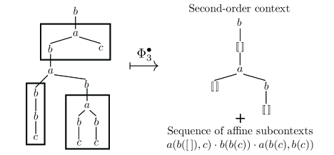
Figure 4. An example of tree decomposition. The parts surrounded by rectangles on the lefthand side show the extracted affine contexts, and the remaining part of the tree is the second-order tree context.

The rest of the section is organized as follows. Before we jump to the decomposition of ${\mathcal{L}}_{n}\!\left({\mathcal{G}},N\right)$, we first present a decomposition of ${\mathcal{T}}_{n}(\Sigma)$, i.e., the set of $\Sigma$-trees of size $n$ in Section 3.2. The decomposition of ${\mathcal{T}}_{n}(\Sigma)$ may be a special case of that of ${\mathcal{L}}_{n}\!\left({\mathcal{G}},N\right)$, where ${\mathcal{G}}$ generates all the trees in ${\mathcal{T}}_{n}(\Sigma)$. For a technical convenience in extending the decomposition of ${\mathcal{T}}_{n}(\Sigma)$ to that of ${\mathcal{L}}_{n}\!\left({\mathcal{G}},N\right)$, we normalize grammars to canonical form in Section 3.3. We then give the decomposition of ${\mathcal{L}}_{n}\!\left({\mathcal{G}},N\right)$ given in Equation (1) above, and prove that it satisfies the required properties in Sections 3.4 and 3.5. Finally, we prove Theorem 6 in Section 3.6.

3.2. Grammar-Independent Tree Decomposition

In this subsection, we will define a decomposition function $\Phi_{m}^{\bullet}$ (where $m$ is a parameter) that decomposes a tree $T$ into (i) a (sufficiently long) sequence $P=U_{1}\cdots U_{k}$ consisting of affine subcontexts of size no less than $m$, and (ii) a “second-order” context $E$ (defined shortly in Section 3.2.1), which is the remainder of extracting $P$ from $T$. Recall Figure 4, which illustrates how a tree is decomposed by $\Phi_{3}^{\bullet}$. Here, the symbol $\llbracket\,\rrbracket$ in the second-order context on the right-hand side represents the original position of each subcontext. By filling the $i$-th occurrence (counted in the depth-first, left-to-right pre-order) of $\llbracket\,\rrbracket$ with the $i$-th affine context, we can recover the original tree on the left hand side.

As formally stated later (in Corollary 16), the decomposition function $\Phi_{m}^{\bullet}$ provides a witness for a bijection of the form

$${\mathcal{T}}_{n}(\Sigma)\cong\coprod_{E\in\mathcal{E}}\prod_{j=1}^{c_{E}}\mathcal{U}_{E,j},$$

a special case of Equation (1) mentioned in Section 3.1.

3.2.1. Second-Order Contexts

We first define the notion of second-order contexts and operations on them.

The set of second-order contexts over $\Sigma$, ranged over by $E$, is defined by:

$$E::=\llbracket\,\rrbracket_{k}^{n}[E_{1},\ldots,E_{k}]\;\mid\;a(E_{1},\ldots,E_{\Sigma(a)})\ \ (a\in\mathop{\mathrm{Dom}}(\Sigma)).$$

Intuitively, the second-order context is an expression having holes of the form $\llbracket\,\rrbracket_{k}^{n}$ (called second-order holes), which should be filled with a $k$-context of size $n$. By filling all the second-order holes, we obtain a $\Sigma$-tree. Note that $k$ may be $0$. In the technical development below, we only consider second-order holes $\llbracket\,\rrbracket_{k}^{n}$ such that $k$ is $0$ or $1$. We write $\mathtt{shn}(E)$ for the number of the second-order holes in $E$. Note that $\Sigma$-trees can be regarded as second-order contexts $E$ such that $\mathtt{shn}(E)=0$, and vice versa. For $i\leq\mathtt{shn}(E)$, we write $E{\centerdot}i$ for the $i$-th second-order hole (counted in the depth-first, left-to-right pre-order). We define the size $|E|$ by: $|\llbracket\,\rrbracket^{n}_{k}[E_{1},\dots,E_{k}]|\triangleq n+|E_{1}|+\cdots+|E_{k}|$ and $|a(E_{1},\dots,E_{\Sigma(a)})|\triangleq|E_{1}|+\cdots+|E_{\Sigma(a)}|+1$. Note that $|E|$ includes the size of contexts to fill the second-order holes in $E$. The second-order context on the right hand side of Figure 4 is expressed as $E=\mathtt{b}(\llbracket\,\rrbracket_{1}^{3}[\mathtt{a}(\llbracket\,\rrbracket_{0}^{3},\mathtt{b}(\llbracket\,\rrbracket_{0}^{5}))])$, where $\mathtt{shn}(E)=3$, $|E|=14$, $E{\centerdot}1=\llbracket\,\rrbracket_{1}^{3}$, $E{\centerdot}2=\llbracket\,\rrbracket_{0}^{3}$, and $E{\centerdot}3=\llbracket\,\rrbracket_{0}^{5}$.

Next we define the substitution operation on second-order contexts. For a context $C$ and a second-order hole $\llbracket\,\rrbracket^{n}_{k}$, we write $C\mathbin{:}\llbracket\,\rrbracket^{n}_{k}$ if $C$ is a $k$-context of size $n$. Given $E$ and $C$ such that $\mathtt{shn}(E)\geq 1$ and $C\mathbin{:}E{\centerdot}1$, we write $E\llbracket C\rrbracket$ for the second-order context obtained by replacing the leftmost second-order hole of $E$ (i.e., $E{\centerdot}1$) with $C$ (and by interpreting the syntactical bracket $[-]$ as the substitution operation). Formally, it is defined by induction on $E$ as follows:

$$\begin{array}[]{lcl}\left(\llbracket\,\rrbracket^{n}_{k}[E_{1},\ldots,E_{k}]\right)\llbracket C\rrbracket&\triangleq&C[E_{1},\ldots,E_{k}]\\ (a(E_{1},\ldots,E_{\Sigma(a)}))\llbracket C\rrbracket&\triangleq&a(E_{1},\ldots,E_{i}\llbracket C\rrbracket,\ldots,E_{\Sigma(a)})\\ &&\hfill\text{ where }i=\min\{j\mid\mathtt{shn}(E_{j})\geq 1,1\leq j\leq\Sigma(a)\}.\end{array}$$

In the first clause, $C[E_{1},\ldots,E_{k}]$ is the second-order context obtained by replacing $[\,]_{i}$ in $C$ with $E_{i}$ for each $i\leq k$. Note that we have $|E\llbracket C\rrbracket|=|E|$ whenever $E\llbracket C\rrbracket$ is well-defined, i.e., if $C\mathbin{:}E{\centerdot}1$ (cf. Lemma 13 below).

We extend the substitution operation for a sequence of contexts. We use metavariable $P$ for sequences of contexts. For $E$ and $P=C_{1}C_{2}\cdots C_{\mathtt{shn}(E)}$, we write $P\mathbin{:}E$ if $C_{i}\mathbin{:}E{\centerdot}i$ for each $i\leq\mathtt{shn}(E)$. Given $E$ and a sequence of contexts $P=C_{1}C_{2}\cdots C_{\ell}$ such that $\ell\leq\mathtt{shn}(E)$ and $C_{i}\mathbin{:}E{\centerdot}i$ for each $i\leq\ell$, we define $E\llbracket P\rrbracket$ by induction on $P$:

$$E\llbracket\epsilon\rrbracket\triangleq E E\llbracket C\cdot P\rrbracket\triangleq(E\llbracket C\rrbracket)\llbracket P\rrbracket$$

Note that $\mathtt{shn}(E\llbracket C\rrbracket)=\mathtt{shn}(E)-1$, so if $P\mathbin{:}E$ then $E\llbracket P\rrbracket$ is a tree.

Recall the second-order context $E=\mathtt{b}(\llbracket\,\rrbracket_{1}^{3}[\mathtt{a}(\llbracket\,\rrbracket_{0}^{3},\mathtt{b}(\llbracket\,\rrbracket_{0}^{5}))])$ in Figure 4 and Example 3.2.1. Let $P$ be the sequence of affine contexts given in Figure 4:

$$\mathtt{a}(\mathtt{b}([\,]),\mathtt{c})\cdot\mathtt{b}(\mathtt{b}(\mathtt{c}))\cdot\mathtt{a}(\mathtt{b}(\mathtt{c}),\mathtt{b}(\mathtt{c})).$$

Then

$$E\llbracket P{\centerdot}1\rrbracket=\mathtt{b}(P{\centerdot}1[\mathtt{a}(\llbracket\,\rrbracket_{0}^{3},\mathtt{b}(\llbracket\,\rrbracket_{0}^{5}))])=\mathtt{b}(\mathtt{a}(\mathtt{b}(\mathtt{a}(\llbracket\,\rrbracket_{0}^{3},\mathtt{b}(\llbracket\,\rrbracket_{0}^{5}))),\mathtt{c})),$$

and

$$E\llbracket P\rrbracket =((E\llbracket P{\centerdot}1\rrbracket])\llbracket P{\centerdot}2\rrbracket)\llbracket P{\centerdot}3\rrbracket$$

$$=\mathtt{b}(\mathtt{a}(\mathtt{b}(\mathtt{a}(P{\centerdot}2,\mathtt{b}(P{\centerdot}3))),\mathtt{c}))=\mathtt{b}(\mathtt{a}(\mathtt{b}(\mathtt{a}(\mathtt{b}(\mathtt{b}(\mathtt{c})),\mathtt{b}(\mathtt{a}(\mathtt{b}(\mathtt{c}),\mathtt{b}(\mathtt{c}))))),\mathtt{c})),$$

which is the tree shown on the left hand side of Figure 4.

Thanks to the size annotation, the substitution operation preserves the size of a second-order context.

Lemma 13.

Let $E$ be a second-order context and $P$ be a sequence of contexts such that $P\mathbin{:}E$. Then $|E|=|E\llbracket P\rrbracket|$.

Proof 3.2.

The proof is given by a straightforward induction on $E$. In the case $E=\llbracket\,\rrbracket_{k}^{n}[E_{1},\ldots,E_{k}]$, we use the fact $|C[E_{1},\ldots,E_{k}]|=|C|+|E_{1}|+\cdots+|E_{k}|$ (which can be shown by induction on $C$).

3.2.2. Grammar-Independent Decomposition Function

Now we define the decomposition function $\Phi_{m}^{\bullet}$. Let $\Sigma$ be a ranked alphabet and $m\geq 1$. We define $r_{\Sigma}\triangleq\max(\mathrm{Im}\left(\Sigma\right))$, which is also written as $r$ for short. We always assume that $r\geq 1$, since it holds whenever $\#\!\left({\mathcal{L}}\!\left({\mathcal{G}}\right)\right)=\infty$, which is an assumption of Theorem 6. We shall define the decomposition function $\Phi_{m}^{\bullet,\Sigma}$ (we omit $\Sigma$ and just write $\Phi_{m}^{\bullet}$ for $\Phi_{m}^{\bullet,\Sigma}$below) so that $\Phi_{m}^{\bullet}(T)=(E,P)$ where (i) $E$ is the second-order context, and (ii) $P$ is a sequence of affine contexts, (iii) $E\llbracket P\rrbracket=T$, and (iv) $m\leq|P{\centerdot}i|\leq r(m-1)+1$ for each $i\in\{1,\ldots,\#\!\left(P\right)\}$.

The function $\Phi_{m}^{\bullet}$ is defined as follows, using an auxiliary decomposition function $\Phi_{m}$ given below.

$$\Phi_{m}^{\bullet}(T)\triangleq(U[E],P)\mbox{ where }(U,E,P)=\Phi_{m}(T).$$

The auxiliary decomposition function (just called “decomposition function” below) $\Phi_{m}$ traverses a given tree $T$ in a bottom-up manner, extracts a sequence $P$ of subcontexts, and returns it along with a linear context $U$ and a second-order context $E$; $U$ and $E$ together represent the “remainder” of extracting $P$ from $T$. During the bottom-up traversal, the $U$-component for each subtree $T^{\prime}$ represents a context containing the root of $T^{\prime}$; whether it is extracted as (a part of) a subcontext or becomes a part of the remainder will be decided later based on the surrounding context. The $E$-component will stay as a part of the remainder during the decomposition of the whole tree (unless the current subtree $T^{\prime}$ is too small, i.e., $|T^{\prime}|<m$).

We define $\Phi_{m}$ by:

• If $|T|<m$, then $\Phi_{m}(T)\triangleq([\,],T,\epsilon)$.

• If $|T|\geq m$, $T=a(T_{1},\ldots,T_{\Sigma(a)})$, and $\Phi_{m}(T_{i})=(U_{i},E_{i},P_{i})\ (\mbox{for each }i\leq\Sigma(a))$, then:

  $$\Phi_{m}(T)\triangleq\left\{\begin{aligned} &([\,],\;a\bigl{(}U_{1}[E_{1}],\dots,U_{\Sigma(a)}[E_{\Sigma(a)}]\bigr{)},\;P_{1}\cdots P_{\Sigma(a)})\\ &\quad\mbox{if there exist $i,j$ such that $1\leq i<j\leq\Sigma(a)$ and $|T_{i}|,|T_{j}|\geq m$}\\ &([\,],\;\llbracket\,\rrbracket^{n}_{1}[E_{i}],\;a(T_{1},\ldots,U_{i},\ldots,T_{\Sigma(a)})\cdot P_{i})\\ &\quad\mbox{if $|T_{j}|<m$ for every $j\neq i$, $|T_{i}|\geq m$, and}\\ &\quad\mbox{\phantom{if} $n\triangleq|a(T_{1},\ldots,U_{i},\ldots,T_{\Sigma(a)})|\geq m$}\\ &(a(T_{1},\ldots,U_{i},\ldots,T_{\Sigma(a)}),\;E_{i},\;P_{i})\\ &\quad\mbox{if $|T_{j}|<m$ for every $j\neq i$, $|T_{i}|\geq m$, and}\\ &\quad\mbox{\phantom{if} $|a(T_{1},\ldots,U_{i},\ldots,T_{\Sigma(a)})|<m$}\\ &([\,],\;\llbracket\,\rrbracket^{n}_{0},\;T)\\ &\quad\mbox{if $|T_{i}|<m$ for every $i\leq\Sigma(a)$, and $n\triangleq|T|$ }\end{aligned}\right.$$ (2)

As defined above, the decomposition is carried out by case analysis on the size of a given tree. If $T$ is not large enough (i.e., $|T|<m$), then $\Phi_{m}(T)$ returns an empty sequence of contexts, while keeping $T$ in the $E$-component. If $|T|\geq m$, then $\Phi_{m}(T)$ returns a non-empty sequence of contexts, by case analysis on the sizes of $T$’s subtrees. If there are more than one subtree whose size is no less than $m$ (the first case above), then $\Phi_{m}(T)$ concatenates the sequences of contexts extracted from the subtrees, and returns the remainder as the second-order context. If only one of the subtrees, say $T_{i}$, is large enough (the second and third cases), then it basically returns the sequence $P_{i}$ extracted from $T_{i}$; however, if the remaining part $a(T_{1},\ldots,U_{i},\ldots,T_{\Sigma(a)})$ is also large enough, then it is added to the sequence (the second case). If none of the subtrees is large enough (but $T$ is large enough), then $T$ is returned as the $P$-component (the last case).

Recall Figure 4. Let $T_{0}$ be the tree on the left hand side. For some of the subtrees of $T_{0}$, $\Phi_{3}$ can be calculated as follows.

$$\begin{array}[]{l}\Phi_{3}(\mathtt{b}(\mathtt{c}))=([\,],\mathtt{b}(\mathtt{c}),\epsilon)\\ \Phi_{3}(\mathtt{b}(\mathtt{b}(\mathtt{c})))=([\,],\llbracket\,\rrbracket_{0}^{3},\mathtt{b}(\mathtt{b}(\mathtt{c})))\hfill\mbox{ (by the last case of~{}\eqref{eq:defOfDecomp})}\\ \Phi_{3}(\mathtt{a}(\mathtt{b}(\mathtt{c}),\mathtt{b}(\mathtt{c})))=([\,],\llbracket\,\rrbracket_{0}^{5},\mathtt{a}(\mathtt{b}(\mathtt{c}),\mathtt{b}(\mathtt{c})))\qquad\hfill\mbox{ (by the last case of~{}\eqref{eq:defOfDecomp})}\\ \Phi_{3}(\mathtt{a}(\mathtt{b}(\mathtt{b}(\mathtt{c})),\mathtt{b}(\cdots)))=([\,],\mathtt{a}(\llbracket\,\rrbracket_{0}^{3},\mathtt{b}(\llbracket\,\rrbracket_{0}^{5})),\mathtt{b}(\mathtt{b}(\mathtt{c}))\cdot\mathtt{a}(\mathtt{b}(\mathtt{c}),\mathtt{b}(\mathtt{c})))\\ \hfill\mbox{ (by the first case of~{}\eqref{eq:defOfDecomp})}\\ \Phi_{3}(T_{0})=(\mathtt{b}([\,]),\llbracket\,\rrbracket_{1}^{3}[\mathtt{a}(\llbracket\,\rrbracket_{0}^{3},\mathtt{b}(\llbracket\,\rrbracket_{0}^{5}))],\mathtt{a}(\mathtt{b}([\,]),\mathtt{c})\cdot\mathtt{b}(\mathtt{b}(\mathtt{c}))\cdot\mathtt{a}(\mathtt{b}(\mathtt{c}),\mathtt{b}(\mathtt{c})))\\ \hfill\mbox{ (by the third case of~{}\eqref{eq:defOfDecomp})}\\ \end{array}$$

From $\Phi_{3}(T_{0})$ above, we obtain:

$$\Phi_{3}^{\bullet}(T_{0})=\left(\mathtt{b}(\llbracket\,\rrbracket_{1}^{3}[\mathtt{a}(\llbracket\,\rrbracket_{0}^{3},\mathtt{b}(\llbracket\,\rrbracket_{0}^{5}))]),\ \mathtt{a}(\mathtt{b}([\,]),\mathtt{c})\cdot\mathtt{b}(\mathtt{b}(\mathtt{c}))\cdot\mathtt{a}(\mathtt{b}(\mathtt{c}),\mathtt{b}(\mathtt{c}))\right).$$

3.2.3. Properties of the Decomposition Function

We summarize important properties of $\Phi_{m}$ in this subsection.

We say that an affine context $U$ is good for $m$ if $|U|\geq m$ and $U$ is of the form $a(U_{1},\dots,U_{\Sigma(a)})$ where $|U_{i}|<m$ for each $i\leq\Sigma(a)$. In other words, $U$ is good if $U$ is of an appropriate size: it is large enough (i.e. $|U|\geq m$), and not too large (i.e. the size of any proper subterm is less than $m$). For example, $\mathtt{a}(\mathtt{b}([\,]),\mathtt{b}(\mathtt{c}))$ is good for $3$, but neither $\mathtt{b}(\mathtt{b}([\,]))$ nor $\mathtt{a}(\mathtt{b}([\,]),\mathtt{b}(\mathtt{b}(\mathtt{c})))$ is.

The following are basic properties of the auxiliary decomposition function $\Phi_{m}$. The property (1) says that the original tree can be recovered by composing the elements obtained by the decomposition, and the property (3) ensures that $\Phi_{m}^{\bullet}(T)$ extracts only good contexts from $T$.

Lemma 14.

Let T be a tree. If $\Phi_{m}(T)=(U,E,P)$, then:

1. $P\mathbin{:}E$,  $\mathtt{hn}(U)=1$, and $(U[E])\llbracket P\rrbracket=T$.

2. $|U|<m$.

3. For each $i\in\{1,\dots,\#\!\left(P\right)\}$, $P{\centerdot}i$ is good for $m$.

4. $|T|=|U[E]|$.

Proof 3.3.

(1)–(3) follow by straightforward simultaneous induction on $|T|$. (4) follows from (1) and Lemma 13.

The following lemma ensures that $\mathtt{shn}(E)$ is sufficiently large whenever $\Phi_{m}^{\bullet}(T)=(E,P)$. Recall condition (ii) of (T3) in Section 3.1; $\mathtt{shn}(E)$ corresponds to $c_{E}$.

Lemma 15.

For any tree $T$ and $m$ such that $1\leq m\leq|T|$, if $\Phi_{m}(T)=(U,E,P)$, then

$$\#\!\left(P\right)\geq\frac{|T|}{2rm}.$$

Proof 3.4.

Recall that $r\triangleq\max(\mathrm{Im}\left(\Sigma\right))$ and we assume $r\geq 1$. We show below that

$$|U|+2rm\#\!\left(P\right)-rm\geq|T|$$

by induction on $T$. Then it follows that

$$2rm\#\!\left(P\right)\geq|T|+rm-|U|>|T|+rm-m\geq|T|$$

(where the second inequality uses Lemma 14(2)), which implies $\#\!\left(P\right)>\frac{\mathchoice{|T|}{|T|}{|T|}{{\scriptstyle|T|}}}{\mathchoice{2rm}{2rm}{2rm}{{\scriptstyle 2rm}}}$ as required.

Since $|T|\geq m$, $\Phi_{m}(T)$ is computed by Equation (2), on which we perform a case analysis. Let $T=a(T_{1},\dots,T_{\Sigma(a)})$ and $\Phi_{m}(T_{i})=(U_{i},E_{i},P_{i})\ (i\leq\Sigma(a))$.

• The first case: In this case, we have

  $$U=[\,]\qquad P=P_{i_{1}}P_{i_{2}}\cdots P_{i_{s}}$$

  where $\{i_{1},\dots,i_{s}\}=\{i\leq\Sigma(a)\mid|T_{i}|\geq m\}$ and $s\geq 2$, since if $|T_{i}|<m$ then $P_{i}=\epsilon$. Note that we have $r\geq 2$ in this case. Then,

  $$|U|+2rm\#\!\left(P\right)-rm$$

  $$=\ 2rm\left(\textstyle\sum_{j\leq s}\#\!\left(P_{i_{j}}\right)\right)-rm$$

  $$\geq\ \left(\textstyle\sum_{j\leq s}(|T_{i_{j}}|+rm-|U_{i_{j}}|)\right)-rm\qquad(\because\text{by induction hypothesis for $T_{i_{j}}$})$$

  $$\geq\ \left(\textstyle\sum_{j\leq s}(|T_{i_{j}}|+rm-(m-1))\right)-rm\qquad(\because|U_{i_{j}}|\leq m-1\mbox{ by Lemma~{}\ref{lemma:charphi}(\ref{charphi:garbagesize})})$$

  $$=\ \left(\textstyle\sum_{j\leq s}|T_{i_{j}}|\right)+srm-sm+s-rm$$

  $$\geq\ \left(\textstyle\sum_{j\leq s}|T_{i_{j}}|\right)+2rm-sm+s-rm-r+1\qquad(\because\text{$s\geq 2$ and $r\geq 1$})$$

  $$=\ \left(\textstyle\sum_{j\leq s}|T_{i_{j}}|\right)+(r-s)(m-1)+1$$

  $$\geq\ \left(\textstyle\sum_{j\leq s}|T_{i_{j}}|\right)+(\Sigma(a)-s)(m-1)+1\qquad(\because r\geq\Sigma(a))$$

  $$\geq\ \left(\textstyle\sum_{j\leq s}|T_{i_{j}}|\right)+(\textstyle\sum_{i\in\{1,\ldots,\Sigma(a)\}\setminus\{i_{1},\ldots,i_{s}\}}|T_{i}|)+1$$

  $$\qquad(\because m-1\geq|T_{i}|\mbox{ for }i\in\{1,\ldots,\Sigma(a)\}\setminus\{i_{1},\ldots,i_{s}\})$$

  $$=\ |T|$$

  as required.

• The second case: In this case, we have

  $$U=[\,]\qquad P=a(T_{1},\ldots,U_{i},\ldots,T_{\Sigma(a)})P_{i}$$

  and $|T_{j}|\geq m$ if and only if $j=i$. Also we have $r\geq 1$. Then,

  $$|U|+2rm\#\!\left(P\right)-rm$$

  $$=\ 2rm(1+\#\!\left(P_{i}\right))-rm$$

  $$=\ rm+2rm\#\!\left(P_{i}\right)$$

  $$\geq\ rm+(|T_{i}|+rm-|U_{i}|)\qquad(\because\text{by induction hypothesis for $T_{i}$})$$

  $$\geq\ |T_{i}|+rm-(m-1)\qquad(\because rm\geq 0,|U_{i}|\leq m-1\mbox{ by Lemma~{}\ref{lemma:charphi}(\ref{charphi:garbagesize})})$$

  $$\geq\ |T_{i}|+rm-r-m+2\qquad(\because r\geq 1)$$

  $$=\ |T_{i}|+(r-1)(m-1)+1$$

  $$\geq\ |T_{i}|+(\Sigma(a)-1)(m-1)+1\qquad(\because r\geq\Sigma(a))$$

  $$\geq\ |T_{i}|+(\textstyle\sum_{j\in\{1,\ldots,\Sigma(a)\}\setminus\{i\}}|T_{j}|)+1$$

  $$=\ |T|$$

  as required.

• The third case of (2): In this case, we have

  $$U=a(T_{1},\ldots,U_{i},\ldots,T_{\Sigma(a)})\qquad P=P_{i}$$

  and $|T_{j}|\geq m$ if and only if $j=i$. Then,

  $$|U|+2rm\#\!\left(P\right)-rm$$

  $$=\ 1+(\textstyle\sum_{j\neq i}|T_{j}|)+|U_{i}|+2rm\#\!\left(P_{i}\right)-rm$$

  $$\geq\ 1+(\textstyle\sum_{j\neq i}|T_{j}|)+|T_{i}|\qquad(\because\text{by induction hypothesis for $T_{i}$})$$

  $$=\ |T|$$

  as required.

• The fourth case of (2): In this case, we have

  $$U=[\,]\qquad P=T.$$

  Then

  $$|U|+2rm\#\!\left(P\right)-rm$$

  $$=\ rm$$

  $$\geq\ r(m-1)+1\qquad(\because r\geq 1)$$

  $$\geq\ \Sigma(a)(m-1)+1\qquad(\because r\geq\Sigma(a))$$

  $$\geq\ (\textstyle\sum_{j\in\{1,\ldots,\Sigma(a)\}}|T_{j}|)+1$$

  $$=\ |T|$$

  as required.

3.2.4. Decomposition of ${\mathcal{T}}_{n}(\Sigma)$

This subsection shows that the decomposition function $\Phi_{m}^{\bullet}$ above provides a witness for a bijection of the form

$${\mathcal{T}}_{n}(\Sigma)\cong\coprod_{E\in\mathcal{E}}\prod_{j=1}^{c_{E}}\mathcal{U}_{E,\,j}.$$

We prepare some definitions to precisely state the bijection. We define the set $\mathcal{E}_{n}^{m}$ of second-order contexts and the set $\mathcal{U}^{m}_{\llbracket\,\rrbracket_{k}^{n}}$ of affine contexts by:

$$\mathcal{E}_{n}^{m} \triangleq\{E\mid(E,P)=\Phi_{m}^{\bullet}(T)\text{ for some }T\in{\mathcal{T}}_{n}(\Sigma)\text{ and }P\}$$

$$\mathcal{U}^{m}_{\llbracket\,\rrbracket_{k}^{n}} \triangleq\{U\mid U:\llbracket\,\rrbracket_{k}^{n},U\text{ is good for }m\}.$$

Intuitively, $\mathcal{E}_{n}^{m}$ is the set of second-order contexts obtained by decomposing a tree of size $n$, and $\mathcal{U}^{m}_{\llbracket\,\rrbracket_{k}^{n}}$ is the set of good contexts that match the second-order context $\llbracket\,\rrbracket_{k}^{n}$.

The bijection is then stated as the following lemma.

Lemma 16.

$${\mathcal{T}}_{n}(\Sigma)\;\cong\coprod_{E\in\mathcal{E}_{n}^{m}}\prod_{i=1}^{\mathtt{shn}(E)}\mathcal{U}^{m}_{E{\centerdot}i}.$$ (3)

The rest of this subsection is devoted to a proof of the lemma above; readers may wish to skip the rest of this subsection upon the first reading.

Lemma 17.

If $E\in\mathcal{E}_{n}^{m}$, then $|E|=n$.

Proof 3.5.

Suppose $E\in\mathcal{E}_{n}^{m}$. Then $(E,P)=\Phi_{m}^{\bullet}(T)$ for some $T\in{\mathcal{T}}_{n}(\Sigma)$ and $P$. By Lemma  14(4), $|E|=|T|=n$.

For a second-order context $E$, and $m\geq 1$, we define the set $\mathcal{P}_{E}^{m}$ of sequences of affine contexts:

$$\mathcal{P}_{E}^{m} \triangleq\{P\mid(E,P)=\Phi_{m}^{\bullet}(T)\text{ for some }T\in{\mathcal{T}}(\Sigma)\}.$$

The set $\mathcal{P}_{E}^{m}$ consists of sequences $P$ of affine contexts that match $E$ and are obtained by the decomposition function $\Phi_{m}^{\bullet}$. In the rest of this subsection, we prove the bijection in Lemma 16 in two steps. We first show ${\mathcal{T}}_{n}(\Sigma)\cong\coprod_{E\in\mathcal{E}_{n}^{m}}\mathcal{P}_{E}^{m}$ (Lemma 18, called “coproduct lemma”), and then show $\mathcal{P}_{E}^{m}=\prod_{j=1}^{\mathtt{shn}(E)}\mathcal{U}^{m}_{E{\centerdot}j}$ (Lemma 18, called “product lemma”).

Lemma 18 (Coproduct Lemma (for Grammar-Independent Decomposition)).

For any $n\geq 1$ and $m\geq 1$, there exists a bijection

$${\mathcal{T}}_{n}(\Sigma)\cong\coprod_{E\in\mathcal{E}_{n}^{m}}\mathcal{P}_{E}^{m}$$

that maps each element $(E,P)$ of the set $\coprod_{E\in\mathcal{E}_{n}^{m}}\mathcal{P}_{E}^{m}$ to $E\llbracket P\rrbracket\in{\mathcal{T}}_{n}(\Sigma)$.

Proof 3.6.

We define a function

$$f:\coprod_{E\in\mathcal{E}_{n}^{m}}\mathcal{P}_{E}^{m}\longrightarrow{\mathcal{T}}_{n}(\Sigma)$$

by $f(E,P)\triangleq E\llbracket P\rrbracket$, and a function

$$g:{\mathcal{T}}_{n}(\Sigma)\longrightarrow\coprod_{E\in\mathcal{E}_{n}^{m}}\mathcal{P}_{E}^{m}$$

by $g(T)\triangleq\Phi_{m}^{\bullet}(T)$.

Let us check that these are functions into the codomains:

• $f(E,P)\in{\mathcal{T}}_{n}(\Sigma)$: Since $P\in\mathcal{P}_{E}^{m}$, there exists $T\in{\mathcal{T}}(\Sigma)$ such that $(E,P)=\Phi_{m}^{\bullet}(T)$. By Lemma 14(1), we have $f(E,P)=E\llbracket P\rrbracket=T\in{\mathcal{T}}(\Sigma)$. By the condition $E\in\mathcal{E}_{n}^{m}$ and by Lemmas 13 and 17, $|E\llbracket P\rrbracket|=|E|=n$. Thus, $f(E,P)\in{\mathcal{T}}_{n}(\Sigma)$ as required.

• $g(T)\in\coprod_{E\in\mathcal{E}_{n}^{m}}\mathcal{P}_{E}^{m}$: Obvious from the definitions of $\mathcal{E}_{n}^{m}$ and $\mathcal{P}_{E}^{m}$.

We have $f(g(T))=T$ by Lemmas 14(1). Let $(E,P)\in\coprod_{E\in\mathcal{E}_{n}^{m}}\mathcal{P}_{E}^{m}$. By definition, there exists $T\in{\mathcal{T}}(\Sigma)$ such that $(E,P)=\Phi_{m}^{\bullet}(T)$. By using Lemmas 13 and 17 again, we have $|T|=|E\llbracket P\rrbracket|=|E|=n$. Thus, $(E,P)=g(T)$. Then

$$g(f(E,P))=g(f(g(T))=g(T)=(E,P).$$

It remains to show the product lemma: $\mathcal{P}_{E}^{m}=\prod_{j=1}^{\mathtt{shn}(E)}\mathcal{U}^{m}_{E{\centerdot}j}$. To this end, we prove a few more properties about the auxiliary decomposition function $\Phi_{m}$.

Lemma 19.

If $|T|\geq m$ and $\Phi_{m}(T)=(U,E,P)$, then $|E|\geq m$.

Proof 3.7.

Straightforward induction on $T$.

The following lemma states that, given $\Phi_{m}(U[T])=(U,E,P)$, $P$ is determined only by $T$ ($U$ does not matter); this is because the decomposition is performed in a bottom-up manner.

Lemma 20.

For $m\geq 1$, $E$, $P$, $T$, and a linear context $U$ with $|T|\geq m$ and $|U|<m$, we have $\Phi_{m}(T)=([\,],E,P)$ if and only if $\Phi_{m}(U[T])=(U,E,P)$.

Proof 3.8.

The proof proceeds by induction on $|U|$. If $U=[\,]$ the claim trivially holds. If $U\neq[\,]$, $U$ is of the form $a(T_{1},\dots,U_{i},\dots,T_{\Sigma(a)})$. Since $|U|<m$, we have $|U_{i}|<m$ and $|T_{j}|<m$ for every $j\neq i$.

Assume that $\Phi_{m}(T)=([\,],E,P)$. By the induction hypothesis, we have $\Phi_{m}(U_{i}[T])=(U_{i},E,P)$. Since $|U|=|a(T_{1},\dots,T_{i-1},U_{i},T_{i+1},\dots,T_{\Sigma(a)})|<m$, we should apply the third case of Equation (2) to compute $\Phi_{m}(U[T])$. Hence, we have

$$\Phi_{m}(U[T])=(a(T_{1},\dots,T_{i-1},U_{i},T_{i+1},\dots,T_{\Sigma(a)}),E,P)=(U,E,P).$$

Conversely, assume that

$$\Phi_{m}(U[T])=(U,E,P)=(a(T_{1},\dots,T_{i-1},U_{i},T_{i+1},\dots,T_{\Sigma(a)}),E,P).$$

Let $(U^{\prime}_{i},E^{\prime}_{i},P^{\prime}_{i})=\Phi_{m}(U_{i}[T])$ and $(U^{\prime}_{j},E^{\prime}_{j},P^{\prime}_{j})=\Phi_{m}(T_{j})$ for each $j\neq i$. Then the final step in the computation of $\Phi_{m}(U[T])$ must be the third case; otherwise $U=[\,]$, a contradiction. By the position of the unique hole in $U$, it must be the case that $U=a(T_{1},\dots,T_{i-1},U^{\prime}_{i},T_{i+1},\dots,T_{\Sigma(a)})$, $E=E^{\prime}_{i}$ and $P=P^{\prime}_{i}$. So $(U_{i},E,P)=\Phi_{m}(U_{i}[T])$. By the induction hypothesis, $\Phi_{m}(T)=([\,],E,P)$.

The following is the key lemma for the product lemma, which says that if $(U,E,P)=\Phi_{m}(T)$, the decomposition is actually independent of the $P$-part.

Lemma 21.

If $(U,E,P)=\Phi_{m}(T)$, then $\Phi_{m}(U[E]\llbracket P^{\prime}\rrbracket)=(U,E,P^{\prime})$ for any $P^{\prime}\in\prod_{i=1}^{\mathtt{shn}(E)}\mathcal{U}^{m}_{E{\centerdot}i}$.

Proof 3.9.

The proof proceeds by induction on $|T|(=|U[E]|)$. If $|T|<m$, then $E=T$, hence $\mathtt{shn}(E)=0$. Thus, $P=P^{\prime}=\epsilon$, which implies $\Phi_{m}(U[E]\llbracket P^{\prime}\rrbracket)=\Phi_{m}(T)=(U,E,P)=(U,E,P^{\prime})$.

For the case $|T|\geq m$, we proceed by the case analysis on which rule of Equation (2) was used to compute $(U,E,P)=\Phi_{m}(T)$. Assume that $T=a(T_{1},\dots,T_{\Sigma(a)})$ and $(U_{i},E_{i},P_{i})=\Phi_{m}(T_{i})$ for each $i=1,\dots,\Sigma(a)$. By Lemma 14, we have $P_{i}\mathbin{:}E_{i}$ for each $i$.

• The first case of Equation (2): We have $|T_{j}|,|T_{j^{\prime}}|\geq m$ for some $1\leq j<j^{\prime}\leq\Sigma(a)$, and:

  $$U=[\,]\qquad E=a(U_{1}[E_{1}],\dots,U_{\Sigma(a)}[E_{\Sigma(a)}])\qquad P=P_{1}\cdots P_{\Sigma(a)}.$$

  Since $P,P^{\prime}:E$, we can split $P^{\prime}=P^{\prime}_{1}\cdots P^{\prime}_{\Sigma(a)}$ so that $P^{\prime}_{i}\mathbin{:}E_{i}$ for each $i$. By the induction hypothesis,

  $$\Phi_{m}(U_{i}[E_{i}]\llbracket P^{\prime}_{i}\rrbracket)=(U_{i},E_{i},P^{\prime}_{i})\qquad\mbox{(for each $i=1,\dots,\Sigma(a)$).}$$

  Since $|U_{j}[E_{j}]\llbracket P^{\prime}_{j}\rrbracket|=|U_{j}[E_{j}]|=|T_{j}|\geq m$ and $|U_{j^{\prime}}[E_{j^{\prime}}]\llbracket P^{\prime}_{j^{\prime}}\rrbracket|=|U_{j^{\prime}}[E_{j^{\prime}}]|=|T_{j^{\prime}}|\geq m$ for some $1\leq j<j^{\prime}\leq\Sigma(a)$, we have

  $$\Phi_{m}(U[E\llbracket P^{\prime}\rrbracket]) =\Phi_{m}(a(U_{1}[E_{1}\llbracket P^{\prime}_{1}\rrbracket],\dots,U_{\Sigma(a)}[E_{\Sigma(a)}\llbracket P^{\prime}_{\Sigma(a)}\rrbracket]))$$

  $$=([\,],a(U_{1}[E_{1}],\dots,U_{\Sigma(a)}[E_{\Sigma(a)}]),P^{\prime}_{1}\cdots P^{\prime}_{\Sigma(a)})$$

  $$=(U,E,P^{\prime})$$

  as required.

• The second case of Equation (2): We have $|T_{j}|\geq m$ for a unique $j\in\{1,\dots,\Sigma(a)\}$ and:

  $$n\triangleq|U_{0}|\geq m\qquad U=[\,]\qquad E=\llbracket\,\rrbracket^{n}_{1}[E_{j}]\qquad P=U_{0}\cdot P_{j}$$

  for $U_{0}\triangleq a(T_{1},\dots,T_{j-1},U_{j},T_{j+1},\dots,T_{\Sigma(a)})$. Because $|T_{j}|\geq m$, we have $|E_{j}|\geq m$ by Lemma 19. Now we have $|E_{j}\llbracket P_{j}\rrbracket|=|E_{j}|\geq m$, $|U_{j}|<m$, and $\Phi_{m}(U_{j}[E_{j}\llbracket P_{j}\rrbracket])=\Phi_{m}(T_{j})=(U_{j},E_{j},P_{j})$; hence by Lemma 20, we have $\Phi_{m}(E_{j}\llbracket P_{j}\rrbracket)=([\,],E_{j},P_{j})$. Let $P^{\prime}=U_{0}^{\prime}\cdot P^{\prime\prime}$. By the assumption, $U_{0}^{\prime}\mathbin{:}\llbracket\,\rrbracket^{n}_{1}$ and thus $U_{0}^{\prime}$ is a $1$-context. Also, $U_{0}^{\prime}$ is good for $m$; thus $|U_{0}^{\prime}|\geq m$ and $U^{\prime}_{0}$ is of the form $a^{\prime}(T_{1}^{\prime},\dots,T^{\prime}_{j^{\prime}-1},U^{\prime}_{j^{\prime}},T^{\prime}_{j+1},\dots,T^{\prime}_{\Sigma(a^{\prime})})$ where $|U^{\prime}_{j^{\prime}}|<m$ and $|T^{\prime}_{i}|<m$ for every $i\neq j^{\prime}$. Now we have

  1. $\Phi_{m}(U^{\prime}_{j^{\prime}}[E_{j}]\llbracket P_{j}\rrbracket)=(U^{\prime}_{j^{\prime}},E_{j},P_{j})$ by Lemma 20 and $\Phi_{m}(E_{j}\llbracket P_{j}\rrbracket)=([\,],E_{j},P_{j})$;

  2. $P^{\prime\prime}\in\prod_{i=1}^{\mathtt{shn}(E_{j})}\mathcal{U}^{m}_{E_{j}{\centerdot}i}$ since $P^{\prime}=U_{0}^{\prime}\cdot P^{\prime\prime}\in\prod_{i=1}^{\mathtt{shn}(E)}\mathcal{U}^{m}_{E{\centerdot}i}$ where $E=\llbracket\,\rrbracket^{n}_{1}[E_{j}]$;

  3. $|U^{\prime}_{j^{\prime}}[E_{j}]|\;<\;|U_{0}^{\prime}[E_{j}]|\;=\;n+|E_{j}|\;=\;|E|\;=\;|U[E]|$.

  Therefore, we can apply the induction hypothesis to $U^{\prime}_{j^{\prime}}[E_{j}]$, resulting in

  $$\Phi_{m}(U^{\prime}_{j^{\prime}}[E_{j}]\llbracket P^{\prime\prime}\rrbracket)=(U^{\prime}_{j^{\prime}},E_{j},P^{\prime\prime}).$$

  We have $|U^{\prime}_{j^{\prime}}[E_{j}]|\geq|E_{j}|\geq m$ and $|T^{\prime}_{i}|<m$ for every $i\neq j^{\prime}$. Furthermore

  $$|a^{\prime}(T^{\prime}_{1},\dots,T^{\prime}_{j^{\prime}-1},U^{\prime}_{j^{\prime}},T^{\prime}_{j^{\prime}+1},\dots,T^{\prime}_{\Sigma(a^{\prime})})|\;=\;|U_{0}^{\prime}|\;=\;n\;\geq\;m.$$

  Hence we have

  $$\Phi_{m}(U[E]\llbracket P^{\prime}\rrbracket) =\Phi_{m}(U_{0}^{\prime}[E_{j}]\llbracket P^{\prime\prime}\rrbracket)$$

  $$=\Phi_{m}(a^{\prime}(T^{\prime}_{1},\dots,T^{\prime}_{j^{\prime}-1},U^{\prime}_{j^{\prime}},T^{\prime}_{j^{\prime}+1},\dots,T^{\prime}_{\Sigma(a^{\prime})})[E_{j}]\llbracket P^{\prime\prime}\rrbracket)$$

  $$=\Phi_{m}(a^{\prime}(T^{\prime}_{1},\dots,T^{\prime}_{j^{\prime}-1},U^{\prime}_{j^{\prime}}[E_{j}]\llbracket P^{\prime\prime}\rrbracket,T^{\prime}_{j^{\prime}+1},\dots,T^{\prime}_{\Sigma(a^{\prime})}))$$

  $$=([\,],\llbracket\,\rrbracket^{n}_{1}[E_{j}],U^{\prime}_{0}\cdot P^{\prime\prime})$$

  $$=(U,E,P^{\prime})$$

• The third case of Equation (2): We have $|T_{j}|=|U_{j}[E_{j}]|\geq m$ for a unique $j\in\{1,\dots,\Sigma(a)\}$ (and thus $|T_{i}|<m$ for every $i\neq j$) and:

  $$U=a(T_{1},\dots,T_{j-1},U_{j},T_{j+1},\dots,T_{\Sigma(a)})\qquad|U|<m\qquad E=E_{j}\qquad P=P_{j}.$$

  By the induction hypothesis,

  $$\Phi_{m}(U_{j}[E_{j}]\llbracket P^{\prime}\rrbracket)=(U_{j},E_{j},P^{\prime}).$$

  Since $|T_{i}|<m$ for every $i\neq j$ and $|a(T_{1},\dots,T_{j-1},U_{j},T_{j+1},\dots,T_{\Sigma(a)})|<m$, we have

  $$\Phi_{m}(U[E]\llbracket P^{\prime}\rrbracket) =\Phi_{m}(a(T_{1},\dots,T_{j-1},U_{j}[E_{j}]\llbracket P^{\prime}\rrbracket,T_{j+1},\dots,T_{\Sigma(a)}))$$

  $$=(a(T_{1},\dots,T_{j-1},U_{j},T_{j+1},\dots,T_{\Sigma(a)}),E_{j},P^{\prime})$$

  $$=(U,E,P^{\prime})$$

• The fourth case of Equation (2): Let $n$ be $|T|$; we have $n\geq m$ and:

  $$U=[\,]\qquad E=\llbracket\,\rrbracket^{n}_{0}\qquad P=T.$$

  Since $P^{\prime}:E$, $P^{\prime}$ must be a singleton sequence consisting of a tree, say $T^{\prime}=a^{\prime}(T_{1}^{\prime},\dots,T_{\Sigma(a^{\prime})}^{\prime})$. By the assumption, $T^{\prime}$ is good for $m$. Hence $|T^{\prime}|\geq m$ and $|T_{i}^{\prime}|<m$ for every $i=1,\dots,\Sigma(a^{\prime})$. So

  $$\Phi_{m}(U[E]\llbracket P^{\prime}\rrbracket)\;=\;\Phi_{m}(T^{\prime})\;=\;([\,],\llbracket\,\rrbracket^{n}_{0},T^{\prime})\;=\;(U,E,P^{\prime}).$$

Corollary 22.

If $(E,P)=\Phi_{m}^{\bullet}(T)$, then $\Phi_{m}^{\bullet}(E\llbracket P^{\prime}\rrbracket)=(E,P^{\prime})$ for any $P^{\prime}\in\prod_{i=1}^{\mathtt{shn}(E)}\mathcal{U}^{m}_{E{\centerdot}i}$.

Proof 3.10.

If $(E,P)=\Phi_{m}^{\bullet}(T)$, then $(U,E^{\prime},P)=\Phi_{m}(T)$ and $U[E^{\prime}]=E$ for some $U,E^{\prime}$. Since $\prod_{i=1}^{\mathtt{shn}(E)}\mathcal{U}^{m}_{E{\centerdot}i}=\prod_{i=1}^{\mathtt{shn}(E^{\prime})}\mathcal{U}^{m}_{E^{\prime}{\centerdot}i}$, Lemma 21 implies $\Phi_{m}(E\llbracket P^{\prime}\rrbracket)=\Phi_{m}(U[E^{\prime}]\llbracket P^{\prime}\rrbracket)=(U,E^{\prime},P^{\prime})$. Thus, we have $\Phi_{m}^{\bullet}(E\llbracket P^{\prime}\rrbracket)=(U[E^{\prime}],P^{\prime})=(E,P^{\prime})$ as required.

We are now ready to prove the product lemma.

Lemma 23 (Product Lemma (for Grammar-Independent Decomposition)).

For $E$ and $m\geq 1$, if $\mathcal{P}_{E}^{m}$ is non-empty, then

$$\mathcal{P}_{E}^{m}=\prod_{i=1}^{\mathtt{shn}(E)}\mathcal{U}^{m}_{E{\centerdot}i}.$$

Proof 3.11.

The direction $\subseteq$ follows from the fact that $(E,P)=\Phi_{m}^{\bullet}(T)$ implies $P\mathbin{:}E$ and $P{\centerdot}i$ is good for $m$ (Lemma 14).

We show the other direction. Since $\mathcal{P}_{E}^{m}\neq\emptyset$, there exist $P$ and $T$ such that $\Phi_{m}^{\bullet}(T)=(E,P)$. Let $P^{\prime}\in\prod_{i=1}^{\mathtt{shn}(E)}\mathcal{U}^{m}_{E{\centerdot}i}$. By Corollary 22, we have $\Phi_{m}^{\bullet}(E\llbracket P^{\prime}\rrbracket)=(E,P^{\prime})$. This means that $P^{\prime}\in\mathcal{P}_{E}^{m}$.

Lemma 16 follows as an immediate corollary of Lemmas 18 and 23.

3.3. Grammars in Canonical Form

As a preparation for generalizing the decomposition of ${\mathcal{T}}_{n}(\Sigma)$ (Lemma 16) to that of ${\mathcal{L}}_{n}\!\left({\mathcal{G}},N\right)$, we first transform a given regular tree grammar into canonical form, which will be defined shortly (in Definition 3.3). We prove that the transformation preserves unambiguity and (a weaker version of) strong connectivity.

[Canonical Grammar] A rewriting rule of a regular tree grammar ${\mathcal{G}}$ is in canonical form if it is of the form

$$N\longrightarrow_{\mathcal{G}}a(N_{1},\dots,N_{\Sigma(a)}).$$

A grammar ${\mathcal{G}}=(\Sigma,{\mathcal{N}},{\mathcal{R}})$ is canonical if every rewriting rule is in canonical form.

We transform a given regular tree grammar ${\mathcal{G}}=(\Sigma,{\mathcal{N}},{\mathcal{R}})$ to an equivalent one in canonical form. The idea of the transformation is fairly simple: we replace a rewriting rule

$$N\longrightarrow a(T_{1},\dots,T_{n})\qquad\mbox{($T_{1},\dots,T_{n}$ are $(\Sigma\cup{\mathcal{N}})$-trees)}$$

such that $T_{i}\notin{\mathcal{N}}$ with rules

$$\{\;\;N\longrightarrow a(T_{1},\dots,T_{i-1},N^{\prime},T_{i+1},\dots,T_{n}),\qquad N^{\prime}\longrightarrow T_{i}\;\;\}$$

where $N^{\prime}$ is a fresh nonterminal that does not appear in ${\mathcal{N}}$. After iteratively applying the above transformation, we next replace a rewriting rule of the form $N\longrightarrow N^{\prime}$ with rules

$$\{N_{0}\longrightarrow a(\dots,N^{\prime},\dots)\mid(N_{0}\longrightarrow a(\dots,N,\dots))\in{\mathcal{R}}\}.$$

Again by iteratively applying this transformation, we finally obtain a grammar in canonical form.

The transformation, however, does not preserve strong connectivity. For example, consider the grammar ${\mathcal{G}}=(\{\mathtt{a}\mapsto 2,\mathtt{b}\mapsto 1,\mathtt{c}\mapsto 0\},\{N\},{\mathcal{R}})$ where

$${\mathcal{R}}=\{\;\;N\longrightarrow\mathtt{b}(\mathtt{c}),\qquad N\longrightarrow\mathtt{a}(N,N)\;\;\}.$$

Then the above transformation introduces a nonterminal $N^{\prime}$ as well as rules

$$N\longrightarrow\mathtt{b}(N^{\prime})\qquad\mbox{and}\qquad N^{\prime}\longrightarrow\mathtt{c}.$$

Then $N$ is not reachable from $N^{\prime}$.

Observe that the problem above was caused by a newly introduced nonterminal that generates a single finite tree. To overcome the problem, we introduce a weaker version of strong connectivity called essential strong-connectivity. It requires strong connectivity only for nonterminals generating infinite languages; hence, it is preserved by the above transformation. [Essential Strong-connectivity] Let ${\mathcal{G}}=(\Sigma,{\mathcal{N}},{\mathcal{R}})$ be a regular tree grammar. We say that ${\mathcal{G}}$ is essentially strongly-connected if for any nonterminals $N_{1},N_{2}\in{\mathcal{N}}$ with $\#\!\left({\mathcal{L}}\!\left({\mathcal{G}},N_{1}\right)\right)=\#\!\left({\mathcal{L}}\!\left({\mathcal{G}},N_{2}\right)\right)=\infty$, $N_{2}$ is reachable from $N_{1}$. Note that by the definition, every strongly-connected grammar is also essentially-strongly connected. In the definition above, as well as in the arguments below, nonterminals $N$ with $\#\!\left({\mathcal{L}}\!\left({\mathcal{G}},N\right)\right)=\infty$ play an important role. We write ${{\mathcal{N}}}^{\mathrm{inf}}$ for the subset of ${\mathcal{N}}$ consisting of such nonterminals.

Remark 24.

A regular tree grammar that is essentially strongly-connected can be easily transformed into a strongly-connected grammar, hence the terminology. Let ${\mathcal{G}}$ be an essentially strongly-connected grammar and $N\in{{\mathcal{N}}}^{\mathrm{inf}}$. We say that a nonterminal is inessential if it generates a finite language. Let $N_{0}$ be an inessential nonterminal of a grammar ${\mathcal{G}}$ such that ${\mathcal{L}}\!\left({\mathcal{G}},N_{0}\right)=\{T_{1},\dots,T_{n}\}$. Then by replacing each rule

$$N_{1}\longrightarrow C[N_{0},\ldots,N_{0}]$$

(where $C$ is a $k$-context possibly having nonterminals other than $N_{0}$) with rules

$$\{N_{1}\longrightarrow C[T_{i_{1}},\ldots,T_{i_{k}}]\mid i_{1},\ldots,i_{k}\in\{1,\dots,n\}\},$$

one can remove the inessential nonterminal $N_{0}$ from the grammar. A grammar ${\mathcal{G}}$ is essentially strongly-connected if and only if the grammar ${\mathcal{G}}^{\prime}$ obtained by removing all inessential nonterminals is strongly-connected. This transformation preserves the language in the following sense: writing ${\mathcal{G}}^{\prime}=(\Sigma,{{\mathcal{N}}}^{\mathrm{inf}},{\mathcal{R}}^{\prime})$ for the resulting grammar, we have ${\mathcal{L}}\!\left({\mathcal{G}},N\right)={\mathcal{L}}\!\left({\mathcal{G}}^{\prime},N\right)$ for each $N\in{{\mathcal{N}}}^{\mathrm{inf}}$. Note that the process of erasing inessential nonterminals breaks canonicity; in fact, the class of languages generated by strongly-connected canonical regular tree grammars is a proper subset of that of essentially strongly-connected canonical regular tree grammars.

Recall that the second main theorem (Theorem 6) takes a family $(S_{n})_{n\in{\rm Nature}}$ from ${\mathcal{S}}({\mathcal{G}})=\bigcup_{N,N^{\prime}\in{\mathcal{N}}}{\mathcal{L}}\!\left({\mathcal{G}},N{\Rightarrow}N^{\prime}\right)$. In order to restate the theorem for essentially strongly connected grammars, we need to replace ${\mathcal{S}}({\mathcal{G}})$ with the “essential” version, namely,

$${\mathcal{S}}^{\mathrm{inf}}({\mathcal{G}})\triangleq\bigcup_{N,N^{\prime}\in{{\mathcal{N}}}^{\mathrm{inf}}}{\mathcal{L}}\!\left({\mathcal{G}},N{\Rightarrow}N^{\prime}\right).$$

Lemma 25 (Canonical Form).

Let ${\mathcal{G}}=(\Sigma,{\mathcal{N}},{\mathcal{R}})$ be a regular tree grammar that is unambiguous and strongly connected. Then one can (effectively) construct a grammar ${\mathcal{G}}^{\prime}=(\Sigma,{\mathcal{N}}^{\prime},{\mathcal{R}}^{\prime})$ and a family $(\mathcal{I}_{N})_{N\in{\mathcal{N}}}$ of subsets $\mathcal{I}_{N}\subseteq{\mathcal{N}}^{\prime}$ that satisfy the following conditions:

• ${\mathcal{G}}^{\prime}$ is canonical, unambiguous and essentially strongly-connected.

• ${\mathcal{L}}\!\left({\mathcal{G}},N\right)=\biguplus_{N^{\prime}\in\mathcal{I}_{N}}{\mathcal{L}}\!\left({\mathcal{G}}^{\prime},N^{\prime}\right)$ for every $N\in{\mathcal{N}}$.

• If $\#\!\left({\mathcal{L}}\!\left({\mathcal{G}}\right)\right)=\infty$, then ${\mathcal{S}}({\mathcal{G}})\subseteq{\mathcal{S}}^{\mathrm{inf}}({\mathcal{G}}^{\prime})$.

Proof 3.12.

See Appendix B.

3.4. Decomposition of Regular Tree Languages

This subsection generalizes the decomposition of ${\mathcal{T}}_{n}(\Sigma)$ in Section 3.2:

$${\mathcal{T}}_{n}(\Sigma)\;\cong\coprod_{E\in\mathcal{E}_{n}^{m}}\prod_{i=1}^{\mathtt{shn}(E)}\mathcal{U}^{m}_{E{\centerdot}i}$$

to that of ${\mathcal{L}}_{n}\!\left({\mathcal{G}},N\right)$, and proves a bijection of the following form:

$${\mathcal{L}}_{n}\!\left({\mathcal{G}},N\right)\;\cong\coprod_{\widetilde{E}\in\widetilde{\mathcal{E}}_{n}^{m}({\mathcal{G}},N)}\prod_{i=1}^{\mathtt{shn}(\widetilde{E})}\widetilde{\mathcal{U}}^{m}_{\widetilde{E}{\centerdot}i}({\mathcal{G}}).$$

Here, $\widetilde{E}$ denotes a typed second-order context (which will be defined shortly in Section 3.4.1), each of whose second-order holes $\widetilde{E}{\centerdot}i=\llbracket\,\rrbracket_{\kappa}^{n}$ carries not only the size $n$ but the context type $\kappa$ of a context to be substituted for the hole. Accordingly, we have replaced $\mathcal{U}^{m}_{E{\centerdot}i}$ with $\widetilde{\mathcal{U}}^{m}_{\widetilde{E}{\centerdot}i}({\mathcal{G}})$, which denotes the set of contexts that respect the context type specified by $\widetilde{E}{\centerdot}i$.

In the rest of this subsection, we first define the notion of typed second-order contexts in Section 3.4.1, extend the decomposition function accordingly in Section 3.4.2, and use it to prove the above bijection in Section 3.4.3. Throughout this subsection (i.e., Section 3.4), we assume that ${\mathcal{G}}$ is a canonical and unambiguous grammar. We emphasize here that the discussion in this subsection essentially relies on both unambiguity and canonicity of the grammar. The essential strong connectivity is not required for the results in this subsection; it will be used in Section 3.5, to show that each component $\widetilde{\mathcal{U}}^{m}_{\widetilde{E}{\centerdot}i}({\mathcal{G}})$ contains an affine context that has $S_{\lceil p\log n\rceil}$ as a subcontext (recall condition (i) of (T3) in Section 3.1).

Remark 26.

Note that any deterministic bottom-up tree automaton (without any $\epsilon$-rules)  [21] can be considered an unambiguous canonical tree grammar, by regarding each transition rule $a(q_{1},\ldots,q_{k})\longrightarrow q$ as a rewriting rule $N_{q}\longrightarrow a(N_{q_{1}},\ldots,N_{q_{k}})$. Thus, by the equivalence between the class of tree languages generated by regular tree grammars and the class of those accepted by deterministic bottom-up tree automata, any regular tree grammar can be converted to an unambiguous canonical tree grammar.

3.4.1. Typed Second-Order Contexts

The set of ${\mathcal{G}}$-typed second-order contexts, ranged over by $\widetilde{E}$, is defined by:

$$\widetilde{E}::=\llbracket\,\rrbracket_{N_{1}\cdots N_{k}{\Rightarrow}N}^{n}[\widetilde{E}_{1},\ldots,\widetilde{E}_{k}]\;\mid\;a(\widetilde{E}_{1},\ldots,\widetilde{E}_{\Sigma(a)})\ \ (a\in\mathop{\mathrm{Dom}}(\Sigma)).$$

The subscript $\kappa=(N_{1}\cdots N_{k}{\Rightarrow}N)$ describes the type of first-order contexts that can be substituted for this second-order hole; the superscript $n$ describes the size as before. Hence a (first-order) context $C$ is suitable for filling a second-order hole $\llbracket\,\rrbracket_{\kappa}^{n}$ if $C:\kappa$ and $|C|=n$. We write $C\mathbin{:}\llbracket\,\rrbracket_{\kappa}^{n}$ if $C:\kappa$ and $|C|=n$. The operations such as $\widetilde{E}{\centerdot}i$, $\widetilde{E}\llbracket C\rrbracket$ and $\widetilde{E}\llbracket P\rrbracket$ are defined analogously. For a sequence of contexts $P=C_{1}C_{2}\cdots C_{\ell}$, we write $P\mathbin{:}\widetilde{E}$ if $\#\!\left(P\right)(=\ell)=\mathtt{shn}(\widetilde{E})$ and $C_{i}\mathbin{:}\widetilde{E}{\centerdot}i$ for each $i\leq\mathtt{shn}(\widetilde{E})$.

We define the second-order context typing relation $\vdash\widetilde{E}:N$ inductively by the rules in Figure 5. Intuitively, $\vdash\widetilde{E}:N$ means that $\widetilde{E}\llbracket P\rrbracket\in{\mathcal{L}}\!\left({\mathcal{G}},N\right)$ holds for any $P$ such that $P\mathbin{:}\widetilde{E}$ (as confirmed in Lemma 28 below). As in the case of untyped second-order contexts, we actually use only typed second-order contexts with holes of the form $\llbracket\,\rrbracket_{N_{1}\cdots N_{k}{\Rightarrow}N}^{n}$ where $k$ is $0$ or $1$.

$$\begin{array}[]{cr}\dfrac{\vdash\widetilde{E}_{i}:N_{i}\quad\mbox{(for each $i=1,\dots,k$)}}{\vdash\llbracket\,\rrbracket_{N_{1}\cdots N_{k}{\Rightarrow}N}^{n}[\widetilde{E}_{1},\dots,\widetilde{E}_{k}]:N}&(\text{SC-Hole})\\[25.0pt] \dfrac{(N\longrightarrow a(N_{1},\dots,N_{\Sigma(a)}))\in{\mathcal{R}}\qquad\vdash\widetilde{E}_{i}:N_{i}\quad\mbox{(for each $i=1,\dots,\Sigma(a)$)}}{\vdash a(\widetilde{E}_{1},\dots,\widetilde{E}_{\Sigma(a)}):N}&(\text{SC-Term})\end{array}$$

Figure 5. Typing rules for $\widetilde{E}$

Recall the second-order context $E=\mathtt{b}(\llbracket\,\rrbracket_{1}^{3}[\mathtt{a}(\llbracket\,\rrbracket_{0}^{3},\mathtt{b}(\llbracket\,\rrbracket_{0}^{5}))])$ in Figure 4 and Example 3.2.1. Given the grammar consisting of the rules:

$$A\to\mathtt{a}(B,B)\qquad B\to\mathtt{b}(A)\qquad B\to\mathtt{b}(B)\qquad B\to\mathtt{c},$$

the corresponding typed second-order context $\widetilde{E}$ is:

$$\mathtt{b}(\llbracket\,\rrbracket_{A{\Rightarrow}A}^{3}[\mathtt{a}(\llbracket\,\rrbracket_{{\Rightarrow}B}^{3},\mathtt{b}(\llbracket\,\rrbracket_{{\Rightarrow}A}^{5}))])$$

and we have $\vdash\widetilde{E}:B$. For $P=\mathtt{a}(\mathtt{b}([\,]),\mathtt{c})\cdot\mathtt{b}(\mathtt{b}(\mathtt{c}))\cdot\mathtt{a}(\mathtt{b}(\mathtt{c}),\mathtt{b}(\mathtt{c}))$, we have $P\mathbin{:}\widetilde{E}$, and:

$$\widetilde{E}\llbracket P\rrbracket=\mathtt{b}(\mathtt{a}(\mathtt{b}(\mathtt{a}(\mathtt{b}(\mathtt{b}(\mathtt{c})),\mathtt{b}(\mathtt{a}(\mathtt{b}(\mathtt{c}),\mathtt{b}(\mathtt{c}))))),\mathtt{c}))\in{\mathcal{L}}\!\left({\mathcal{G}},B\right).$$

Lemma 27.

The following rule is derivable:

$$\begin{array}[]{cr}\dfrac{C\in{\mathcal{L}}\!\left({\mathcal{G}},N_{1}\dots N_{k}{\Rightarrow}N\right)\qquad\vdash\widetilde{E}_{i}:N_{i}\quad\mbox{\rm(for each $i=1,\dots,k$)}}{\vdash C[\widetilde{E}_{1},\dots,\widetilde{E}_{k}]:N}&(\mbox{\rm SC-Ctx})\end{array}$$

Proof 3.13.

The proof proceeds by induction on $C$. Assume that the premises of the rule hold. If $C=[\,]$, then $C[\widetilde{E}_{1},\dots,\widetilde{E}_{k}]=\widetilde{E}_{1}$ and $N=N_{1}$; thus the result follows immediately from the assumption. If $C=a(C_{1},\ldots,C_{\ell})$, then by the assumption that the grammar is canonical and $C\in{\mathcal{L}}\!\left({\mathcal{G}},N_{1}\dots N_{k}{\Rightarrow}N\right)$, we have $N\to a(N^{\prime}_{1},\ldots,N^{\prime}_{\ell})$ with $C_{i}\in{\mathcal{L}}\!\left({\mathcal{G}},N_{k_{i-1}+1}\dots N_{k_{i}}{\Rightarrow}N^{\prime}_{i}\right)$ for $i=1,\ldots,\ell$ where $k_{0}=0$ and $k_{\ell}=k$. By the induction hypothesis, we have $\vdash C_{i}[\widetilde{E}_{k_{i-1}+1},\ldots,\widetilde{E}_{k_{i}}]:N^{\prime}_{i}$. Thus, by using rule (SC-Term), we have $\vdash C[\widetilde{E}_{1},\dots,\widetilde{E}_{k}]:N$ as required.

Lemma 28.

Assume that $\vdash\widetilde{E}:N$.

1. If $\mathtt{shn}(\widetilde{E})=0$, then $\widetilde{E}$ is a tree and $\widetilde{E}\in{\mathcal{L}}\!\left({\mathcal{G}},N\right)$.

2. If $\mathtt{shn}(\widetilde{E})\geq 1$ and $C\mathbin{:}\widetilde{E}{\centerdot}1$, then $\vdash\widetilde{E}\llbracket C\rrbracket:N$.

3. If $P\mathbin{:}\widetilde{E}$, then $\widetilde{E}\llbracket P\rrbracket\in{\mathcal{L}}\!\left({\mathcal{G}},N\right)$.

Proof 3.14.

$(1)$ By induction on the structure of $\vdash\widetilde{E}:N$. $(2)$ By induction on the structure of $\vdash\widetilde{E}:N$. The base case is when $\widetilde{E}=\llbracket\,\rrbracket_{N_{1}\dots N_{k}{\Rightarrow}N}^{n}[\widetilde{E}_{1},\dots,\widetilde{E}_{k}]$. Since $\vdash\widetilde{E}:N$, we have $\vdash\widetilde{E}_{i}:N_{i}$ for each $i$. Then by the derived rule (SC-Ctx), we have $\vdash C[\widetilde{E}_{1},\dots,\widetilde{E}_{k}]:N$. $(3)$ By induction on $\mathtt{shn}(\widetilde{E})$ (using $(1)$ and $(2)$).

3.4.2. Grammar-Respecting Decomposition Function $\widetilde{\Phi}_{m}^{\bullet,{\mathcal{G}}}$

We have defined in Section 3.2.2 the function $\Phi_{m}^{\bullet}$ that decomposes a tree $T$ and returns a pair $(E,P)$ of a second-order context $E$ and a sufficiently long sequence $P$ of (first-order) contexts. The aim here is to extend $\Phi_{m}^{\bullet}$ to a grammar-respecting one $\widetilde{\Phi}_{m}^{\bullet,{\mathcal{G}}}$ that takes a pair $(T,N)$ such that $T\in{\mathcal{L}}\!\left({\mathcal{G}},N\right)$ as an input, and returns a pair $(\widetilde{E},P)$, which is the same as $\Phi_{m}^{\bullet}(T)=(E,P)$, except that $\widetilde{E}$ is a “type-annotated” version of $E$. For example, for the tree in Figure 4 and the grammar in Example 3.4.1, we expect that $\widetilde{\Phi}_{m}^{\bullet,{\mathcal{G}}}(T)=(\widetilde{E},P)$ where:

$$\begin{array}[]{l}T=\mathtt{b}(\mathtt{a}(\mathtt{b}(\mathtt{a}(\mathtt{b}(\mathtt{b}(\mathtt{c})),\mathtt{b}(\mathtt{a}(\mathtt{b}(\mathtt{c}),\mathtt{b}(\mathtt{c}))))),\mathtt{c}))\\ \widetilde{E}=\mathtt{b}(\llbracket\,\rrbracket_{A{\Rightarrow}A}^{3}[\mathtt{a}(\llbracket\,\rrbracket_{{\Rightarrow}B}^{3},\mathtt{b}(\llbracket\,\rrbracket_{{\Rightarrow}A}^{5}))])\qquad P=\mathtt{a}(\mathtt{b}([\,]),\mathtt{c})\cdot\mathtt{b}(\mathtt{b}(\mathtt{c}))\cdot\mathtt{a}(\mathtt{b}(\mathtt{c}),\mathtt{b}(\mathtt{c})).\end{array}$$

We say that $\widetilde{E}$ refines $E$, written $\widetilde{E}\lhd E$, if $E$ is obtained by simply forgetting type annotations, i.e., replacing $\llbracket\,\rrbracket_{N_{1}\cdots N_{k}{\Rightarrow}N}^{n}$ in $\widetilde{E}$ with $\llbracket\,\rrbracket_{k}^{n}$. This relation is formally defined by induction on the structures of $E$ and $\widetilde{E}$ by the rules in Figure 6.

$$\begin{array}[]{cr}\dfrac{\widetilde{E}_{i}\lhd E_{i}\quad\mbox{(for each $i=1,\dots,k$)}}{\llbracket\,\rrbracket_{N_{1}\cdots N_{k}{\Rightarrow}N}^{n}[\widetilde{E}_{1},\dots,\widetilde{E}_{k}]\lhd\llbracket\,\rrbracket_{k}^{n}[E_{1},\dots,E_{n}]}&(\text{Ref-Hole})\\[25.0pt] \dfrac{\widetilde{E}_{i}\lhd E_{i}\quad\mbox{(for each $i=1,\dots,\Sigma(a)$)}}{a(\widetilde{E}_{1},\dots,\widetilde{E}_{\Sigma(a)})\lhd a(E_{1},\dots,E_{n})}&(\text{Ref-Term})\end{array}$$

Figure 6. Refinement relation

The following lemma is obtained by straightforward induction on $\widetilde{E}\lhd E$.

Lemma 29.

Assume $\widetilde{E}\lhd E$.

1. $|\widetilde{E}|=|E|$.

2. If $P\mathbin{:}\widetilde{E}$, then $P\mathbin{:}E$.

3. If $P\mathbin{:}\widetilde{E}$, then $\widetilde{E}\llbracket P\rrbracket=E\llbracket P\rrbracket$.

Given $T\in{\mathcal{L}}\!\left({\mathcal{G}},N\right)$ and $(E,P)=\Phi_{m}^{\bullet}(T)$, the value of $\widetilde{\Phi}_{m}^{\bullet,{\mathcal{G}}}(T,N)$ should be $(\widetilde{E},P)$ where $\widetilde{E}$ is a ${\mathcal{G}}$-typed second-order context that satisfies the following conditions:

$$\widetilde{E}\lhd E,\qquad\vdash\widetilde{E}:N\quad\mbox{and}\quad P\mathbin{:}\widetilde{E}.$$

We prove that, for every $T\in{\mathcal{L}}\!\left({\mathcal{G}},N\right)$, there exists exactly one typed second-order context $\widetilde{E}$ that satisfies the above condition. Hence the above constraints define the function $\widetilde{\Phi}_{m}^{\bullet,{\mathcal{G}}}(T,N)$.

We first state and prove a similar result for first-order contexts (in Lemma 30), and then prove the second-order version (in Lemma 31), using the former.

Lemma 30.

Let $C$ be a (first-order) $k$-context and $T_{1},\dots,T_{k}$ be trees. Assume that $C[T_{1},\dots,T_{k}]\in{\mathcal{L}}\!\left({\mathcal{G}},N\right)$. Then there exists a unique family $(N_{i})_{i\in\{1,\dots,k\}}$ such that $C\in{\mathcal{L}}\!\left({\mathcal{G}},N_{1}\dots N_{k}{\Rightarrow}N\right)$ and $T_{i}\in{\mathcal{L}}\!\left({\mathcal{G}},N_{i}\right)$ for every $i=1,\dots,k$.

Proof 3.15.

By induction on $C$.

• Case $C=[\,]$: Then $k=1$. The existence follows from $[\,]\in{\mathcal{L}}\!\left({\mathcal{G}},N{\Rightarrow}N\right)$ (as $N\longrightarrow^{*}N$) and $T_{1}=C[T_{1}]\in{\mathcal{L}}\!\left({\mathcal{G}},N\right)$. The uniqueness follows from the fact that $[\,]\in{\mathcal{L}}\!\left({\mathcal{G}},N_{1}{\Rightarrow}N\right)$ implies $N_{1}=N$.

• Case $C=a(C_{1},\dots,C_{\Sigma(a)})$: Let $\ell=\Sigma(a)$, $k_{i}=\mathtt{hn}(C_{i})$ for each $i=1,\dots,\ell$ and

  $$(T_{1,1},\dots,T_{1,k_{1}},T_{2,1},\dots,T_{2,k_{2}},\dots,T_{\ell,1},\dots,T_{\ell,k_{\ell}})=(T_{1},\dots,T_{k}).$$

  Then $C[T_{1},\dots,T_{k}]=a(C_{1}[T_{1,1},\dots,T_{1,k}],\dots,C_{\ell}[T_{\ell,1},\dots T_{\ell,k_{\ell}}])$. Since $C[T_{1},\dots,T_{k}]\in{\mathcal{L}}\!\left({\mathcal{G}},N\right)$, there exists a rewriting sequence

  $$N\longrightarrow a(N_{1},\dots,N_{\ell})\longrightarrow^{*}a(C_{1}[T_{1,1},\dots,T_{1,k_{1}}],\dots,C_{\ell}[T_{\ell,1},\dots T_{\ell,k_{\ell}}]).$$

  Thus $N_{i}\longrightarrow^{*}C_{i}[T_{i,1},\dots,T_{i,k_{i}}]$, i.e., $C_{i}[T_{i,1},\dots,T_{i,k_{i}}]\in{\mathcal{L}}\!\left({\mathcal{G}},N_{i}\right)$, for each $i=1,\dots,\ell$. By the induction hypothesis, there exist $N_{i,1},\dots,N_{i,k_{i}}$ such that $C_{i}\in{\mathcal{L}}\!\left({\mathcal{G}},N_{i,1}\dots N_{i,k_{i}}{\Rightarrow}N_{i}\right)$ and $T_{i,j}\in{\mathcal{L}}\!\left({\mathcal{G}},N_{i,j}\right)$ for each $j=1,\dots,k_{i}$. Then (the rearrangement of) the family $(N_{i,j})_{i\leq\ell,j\leq k_{i}}$ satisfies the requirement.

  We prove the uniqueness. Assume that both $(N^{1}_{i,j})_{i,j}$ and $(N^{2}_{i,j})_{i,j}$ satisfy the requirement. Then, for each $m=1,2$, there exist $N^{m}_{i}$ ($i=1,\dots,\ell$) such that

  $$N\longrightarrow a(N^{m}_{1},\dots,N^{m}_{\ell}) \longrightarrow^{*}a(C_{1}[N^{m}_{1,1},\dots,N^{m}_{1,k_{1}}],\dots,C_{\ell}[N^{m}_{\ell,1},\dots,N^{m}_{\ell,k_{\ell}}])$$

  $$\longrightarrow^{*}a(C_{1}[T_{1,1},\dots,T_{1,k_{1}}],\dots,C_{\ell}[T_{\ell,1},\dots,T_{\ell,k_{\ell}}]).$$

  Since ${\mathcal{G}}$ is unambiguous, $N^{1}_{i}=N^{2}_{i}$ for each $i=1,\dots,\ell$. By the induction hypothesis, we have $N^{1}_{i,j}=N^{2}_{i,j}$ for each $i$ and $j$.

Lemma 31.

Let ${\mathcal{G}}$ be a canonical unambiguous regular tree grammar and $T\in{\mathcal{L}}\!\left({\mathcal{G}},N\right)$. Given $E$ and $P$, assume that $P\mathbin{:}E$ and $E\llbracket P\rrbracket=T$. Then $E$ has a unique refinement $\widetilde{E}\lhd E$ such that $\vdash\widetilde{E}:N$ and $P\mathbin{:}\widetilde{E}$.

Proof 3.16.

We prove by induction on $E$.

• Case $E=\llbracket\,\rrbracket_{k}^{n}[E_{1},\dots,E_{k}]$: The sequence $P$ can be decomposed as $P=C\cdot P_{1}\cdots P_{k}$ so that $P_{i}\mathbin{:}E_{i}$ for each $i=1,\dots,k$. Furthermore $\mathtt{hn}(C)=k$ and $|C|=n$. We have $E\llbracket P\rrbracket=C[E_{1}\llbracket P_{1}\rrbracket,\dots,E_{k}\llbracket P_{k}\rrbracket]\in{\mathcal{L}}\!\left({\mathcal{G}},N\right)$.

  We prove the existence. By Lemma 30, there exists a family $(N_{i})_{i=1,\dots,k}$ such that $C\in{\mathcal{L}}\!\left({\mathcal{G}},N_{1}\dots N_{k}{\Rightarrow}N\right)$ (i.e., $C:\llbracket\,\rrbracket_{N_{1}\dots N_{k}{\Rightarrow}N}^{n}$) and $E_{i}\llbracket P_{i}\rrbracket\in{\mathcal{L}}\!\left({\mathcal{G}},N_{i}\right)$ for each $i=1,\dots,k$. By the induction hypothesis, for each $i=1,\dots,k$, there exists $\widetilde{E}_{i}\lhd E_{i}$ such that $\vdash\widetilde{E}_{i}:N_{i}$ and $P_{i}\mathbin{:}\widetilde{E}_{i}$. Let $\widetilde{E}\triangleq\llbracket\,\rrbracket_{N_{1}\dots N_{k}{\Rightarrow}N}^{n}[\widetilde{E}_{1},\dots,\widetilde{E}_{k}]$. Then $\widetilde{E}\lhd E$, $\vdash\widetilde{E}:N$, and $P\mathbin{:}\widetilde{E}$.

  We prove the uniqueness. Assume $\widetilde{E}^{1}$ and $\widetilde{E}^{2}$ satisfy that $\widetilde{E}^{j}\lhd E$, $\vdash\widetilde{E}^{j}:N$ and $P\mathbin{:}\widetilde{E}^{j}$ for $j=1,2$. Since $\widetilde{E}^{j}\lhd E$ and $\vdash\widetilde{E}^{j}:N$, $\widetilde{E}^{j}$ must be of the form: $\widetilde{E}^{j}=\llbracket\,\rrbracket_{N_{1}^{j}\dots N_{k}^{j}{\Rightarrow}N}^{n}[\widetilde{E}^{j}_{1},\dots,\widetilde{E}^{j}_{k}]$ with $\widetilde{E}^{j}_{i}\lhd E_{i}$ and $\vdash\widetilde{E}^{j}_{i}:N^{j}_{i}$. Since $P\mathbin{:}\widetilde{E}^{j}$, we have $C\in{\mathcal{L}}\!\left({\mathcal{G}},N_{1}^{j}\dots N_{k}^{j}{\Rightarrow}N\right)$ and $P_{i}:\widetilde{E}^{j}_{i}$ for $i=1,\dots,k$. By Lemma 28, $\widetilde{E}^{j}_{i}\llbracket P_{i}\rrbracket\in{\mathcal{L}}\!\left({\mathcal{G}},N_{i}^{j}\right)$ for each $i=1,\dots,k$ and $j=1,2$. By Lemma 29(3), $E\llbracket P\rrbracket=\widetilde{E}^{j}\llbracket P\rrbracket=C[\widetilde{E}^{j}_{1}\llbracket P_{1}\rrbracket,\dots,\widetilde{E}^{j}_{k}\llbracket P_{k}\rrbracket]\in{\mathcal{L}}\!\left({\mathcal{G}},N\right)$. Hence by Lemma 30, $N_{i}^{1}=N_{i}^{2}$ for each $i=1,\dots,k$. By the induction hypothesis, $\widetilde{E}_{i}^{1}=\widetilde{E}_{i}^{2}$ for each $i$. Hence $\widetilde{E}^{1}=\widetilde{E}^{2}$.

• Case $E=a(E_{1},\dots,E_{\Sigma(a)})$: The sequence $P$ can be decomposed as $P=P_{1}\cdots P_{\Sigma}(a)$ so that $P_{i}\mathbin{:}E_{i}$ for each $i=1,\dots,\Sigma(a)$. Then $E\llbracket P\rrbracket=a(E_{1}\llbracket P_{1}\rrbracket,\dots,E_{\Sigma(a)}\llbracket P_{\Sigma(a)}\rrbracket)$.

  We prove the existence. Since $N\longrightarrow^{*}a(E_{1}\llbracket P_{1}\rrbracket,\dots,E_{\Sigma(a)}\llbracket P_{\Sigma(a)}\rrbracket)$, there exists a rule $N\longrightarrow a(N_{1},\dots,N_{\Sigma(a)})$ such that

  $$N\longrightarrow a(N_{1},\dots,N_{\Sigma(a)})\longrightarrow^{*}a(E_{1}\llbracket P_{1}\rrbracket,\dots,E_{\Sigma(a)}\llbracket P_{\Sigma(a)}\rrbracket).$$

  So $N_{i}\longrightarrow^{*}E_{i}\llbracket P_{i}\rrbracket$ for each $i=1,\dots,\Sigma(a)$. By the induction hypothesis, there exists $\widetilde{E}_{i}\lhd E_{i}$ such that $\vdash\widetilde{E}_{i}:N_{i}$ and $P_{i}\mathbin{:}\widetilde{E}_{i}$. Let $\widetilde{E}\triangleq a(\widetilde{E}_{1},\dots,\widetilde{E}_{\Sigma(a)})$. Then $\widetilde{E}\lhd E$, $\vdash\widetilde{E}:N$, and $P\mathbin{:}\widetilde{E}$.

  We prove the uniqueness. Assume $\widetilde{E}^{1}$ and $\widetilde{E}^{2}$ satisfy that $\widetilde{E}^{j}\lhd E$, $\vdash\widetilde{E}^{j}:N$ and $P\mathbin{:}\widetilde{E}^{j}$ for $j=1,2$. Since $\widetilde{E}^{j}\lhd E$, $\widetilde{E}^{j}$ must be of the form: $\widetilde{E}^{j}=a(\widetilde{E}^{j}_{1},\dots,\widetilde{E}^{j}_{\Sigma(a)})$ with $\widetilde{E}^{j}_{i}\lhd E_{i}$. By $\vdash\widetilde{E}^{j}:N$, there exists a rule $N\longrightarrow a(N_{1}^{j},\dots,N_{\Sigma(a)}^{j})$ such that $\vdash\widetilde{E}^{j}_{i}:N_{i}^{j}$ for each $i$. Since $P:\widetilde{E}^{j}$, we have $P_{i}:\widetilde{E}^{j}_{i}$ for each $i$. By Lemmas 28 and 29(3), we have $\widetilde{E}_{i}^{j}\llbracket P_{i}\rrbracket=E_{i}\llbracket P_{i}\rrbracket\in{\mathcal{L}}\!\left({\mathcal{G}},N_{i}^{j}\right)$. Now we have

  $$N\longrightarrow a(N_{1}^{j},\dots,N_{\Sigma(a)}^{j})\longrightarrow^{*}a(E_{1}\llbracket P_{1}\rrbracket,\dots,E_{\Sigma(a)}\llbracket P_{\Sigma(a)}\rrbracket)$$

  for $j=1,2$. Since ${\mathcal{G}}$ is unambiguous, $N_{i}^{1}=N_{i}^{2}$ for each $i=1,\dots,\Sigma(a)$. By the induction hypothesis, $\widetilde{E}_{i}^{1}=\widetilde{E}_{i}^{2}$ for each $i$. Hence $\widetilde{E}^{1}=\widetilde{E}^{2}$.

3.4.3. Decomposition of ${\mathcal{L}}_{n}\!\left({\mathcal{G}},N\right)$

To formally state the decomposition lemma, we prepare some definitions. For a canonical unambiguous grammar ${\mathcal{G}}=(\Sigma,{\mathcal{N}},{\mathcal{R}})$, $N\in{\mathcal{N}}$, $n\geq 1$, and $m\geq 1$, we define $\widetilde{\mathcal{E}}_{n}^{m}({\mathcal{G}},N)$, $\widetilde{\mathcal{P}}_{\widetilde{E}}^{m}({\mathcal{G}},N)$, and $\widetilde{\mathcal{U}}^{m}_{\llbracket\,\rrbracket_{\kappa}^{n}}({\mathcal{G}})$ by:

$$\widetilde{\mathcal{E}}_{n}^{m}({\mathcal{G}},N) \triangleq\{\widetilde{E}\mid(\widetilde{E},P)=\widetilde{\Phi}_{m}^{\bullet,{\mathcal{G}}}(T,N)\text{ for some }T\in{\mathcal{L}}_{n}\!\left({\mathcal{G}},N\right)\text{ and }P\}.$$

$$\widetilde{\mathcal{P}}_{\widetilde{E}}^{m}({\mathcal{G}},N) \triangleq\{P\mid(\widetilde{E},P)=\widetilde{\Phi}_{m}^{\bullet,{\mathcal{G}}}(T,N)\text{ for some }T\in{\mathcal{L}}\!\left({\mathcal{G}},N\right)\}.$$

$$\widetilde{\mathcal{U}}^{m}_{\llbracket\,\rrbracket_{\kappa}^{n}}({\mathcal{G}}) \triangleq\{U\mid U:\llbracket\,\rrbracket_{\kappa}^{n},U\text{ is good for }m\}.$$

The set $\widetilde{\mathcal{E}}_{n}^{m}({\mathcal{G}},N)$ consists of second-order contexts that are obtained by decomposing trees of size $n$, and $\widetilde{\mathcal{P}}_{\widetilde{E}}^{m}({\mathcal{G}},N)$ consists of affine context sequences that match $\widetilde{E}$. The set $\widetilde{\mathcal{P}}_{\widetilde{E}}^{m}({\mathcal{G}},N)$ is the set of contexts that match the hole $\llbracket\,\rrbracket_{\kappa}^{n}$.

The following is the main result of this subsection.

Lemma 32.

$${\mathcal{L}}_{n}\!\left({\mathcal{G}},N\right)\quad\cong \coprod_{\widetilde{E}\in\widetilde{\mathcal{E}}_{n}^{m}({\mathcal{G}},N)}\prod_{i=1}^{\mathtt{shn}(\widetilde{E})}\widetilde{\mathcal{U}}^{m}_{\widetilde{E}{\centerdot}i}({\mathcal{G}}).$$

The lemma above is a direct consequence of typed versions of coproduct and product lemmas (Lemmas 33 and 35 below). The following coproduct lemma can be shown in a manner similar to Lemma 18:

Lemma 33 (Coproduct Lemma (for Grammar-Respecting Decomposition)).

For any $n\geq 1$ and $m\geq 1$, there exists a bijection

$${\mathcal{L}}_{n}\!\left({\mathcal{G}},N\right)\quad\cong \coprod_{\widetilde{E}\in\widetilde{\mathcal{E}}_{n}^{m}({\mathcal{G}},N)}\widetilde{\mathcal{P}}_{\widetilde{E}}^{m}({\mathcal{G}},N).$$

such that $(\widetilde{E},P)$ in the right hand side is mapped to $\widetilde{E}\llbracket P\rrbracket$.

Proof 3.17.

We define a function

$$f:\coprod_{\widetilde{E}\in\widetilde{\mathcal{E}}_{n}^{m}({\mathcal{G}},N)}\widetilde{\mathcal{P}}_{\widetilde{E}}^{m}({\mathcal{G}},N)\longrightarrow{\mathcal{L}}_{n}\!\left({\mathcal{G}},N\right)$$

by $f(\widetilde{E},P)\triangleq\widetilde{E}\llbracket P\rrbracket$, and a function

$$g:{\mathcal{L}}_{n}\!\left({\mathcal{G}},N\right)\longrightarrow\coprod_{\widetilde{E}\in\widetilde{\mathcal{E}}_{n}^{m}({\mathcal{G}},N)}\widetilde{\mathcal{P}}_{\widetilde{E}}^{m}({\mathcal{G}},N)$$

by $g(T)\triangleq\widetilde{\Phi}_{m}^{\bullet,{\mathcal{G}}}(T,N)$.

Let us check that these are functions into the codomains:

• $f(\widetilde{E},P)\in{\mathcal{L}}_{n}\!\left({\mathcal{G}},N\right)$: Since $P\in\widetilde{\mathcal{P}}_{\widetilde{E}}^{m}({\mathcal{G}},N)$, there exists $T\in{\mathcal{L}}_{n}\!\left({\mathcal{G}},N\right)$ such that $(\widetilde{E},P)=\widetilde{\Phi}_{m}^{\bullet,{\mathcal{G}}}(T,N)$. By Lemmas 14 and 29, we have $f(\widetilde{E},P)=\widetilde{E}\llbracket P\rrbracket=T\in{\mathcal{L}}_{n}\!\left({\mathcal{G}},N\right)$.

• $g(T)\in\coprod_{\widetilde{E}\in\widetilde{\mathcal{E}}_{n}^{m}({\mathcal{G}},N)}\widetilde{\mathcal{P}}_{\widetilde{E}}^{m}({\mathcal{G}},N)$: Obvious from the definitions of $\widetilde{\mathcal{E}}_{n}^{m}({\mathcal{G}},N)$ and $\widetilde{\mathcal{P}}_{\widetilde{E}}^{m}({\mathcal{G}},N)$.

We have $f(g(T))=T$ by Lemmas 14(1) and 29. Let $(\widetilde{E},P)\in\coprod_{\widetilde{E}\in\widetilde{\mathcal{E}}_{n}^{m}({\mathcal{G}},N)}\widetilde{\mathcal{P}}_{\widetilde{E}}^{m}({\mathcal{G}},N)$. By definition, there exists $T\in{\mathcal{L}}_{n}\!\left({\mathcal{G}},N\right)$ such that $(\widetilde{E},P)=\widetilde{\Phi}_{m}^{\bullet,{\mathcal{G}}}{(T,N)}=g(T)$. Then

$$g(f(\widetilde{E},P))=g(f(g(T))=g(T)=(\widetilde{E},P).$$

The following is a key lemma used for proving a typed version of the product lemma.

Lemma 34.

For a nonterminal $N$, $n\geq 1$, $m\geq 1$ and $\widetilde{E}\in\widetilde{\mathcal{E}}_{n}^{m}({\mathcal{G}},N)$, let $E$ be the unique second-order context such that $\widetilde{E}\lhd E$. Then we have

$$\widetilde{\mathcal{P}}_{\widetilde{E}}^{m}({\mathcal{G}},N)=\mathcal{P}_{E}^{m}\cap\{P\mid P\mathbin{:}\widetilde{E}\}.$$

Proof 3.18.

The direction $\subseteq$ is clear. We prove the converse.

Let $P$ be in the right hand side. Since $\widetilde{E}\in\widetilde{\mathcal{E}}_{n}^{m}({\mathcal{G}},N)$, there exist $T^{\prime}$ and $P^{\prime}$ such that

$$\widetilde{\Phi}_{m}^{\bullet,{\mathcal{G}}}(T^{\prime},N)=(\widetilde{E},P^{\prime}).$$

By the definition of $\widetilde{\Phi}_{m}^{\bullet,{\mathcal{G}}}(T^{\prime},N)$, we have $\vdash\widetilde{E}:N$. Since $P\in\mathcal{P}_{E}^{m}$, there exists $T$ such that $(E,P)=\Phi_{m}^{\bullet}(T)$ and thus, by Lemma 14,

$$\Phi_{m}^{\bullet}(E\llbracket P\rrbracket)=(E,P).$$

Since $\Phi_{m}^{\bullet}(E\llbracket P\rrbracket)=(E,P)$, $\widetilde{E}\lhd E$, $\vdash\widetilde{E}:N$, and $P\mathbin{:}\widetilde{E}$, by the definition of $\widetilde{\Phi}_{m}^{\bullet,{\mathcal{G}}}$, we have $\widetilde{\Phi}_{m}^{\bullet,{\mathcal{G}}}(E\llbracket P\rrbracket,N)=(\widetilde{E},P)$. By Lemmas 28(3) and 29(3), $E\llbracket P\rrbracket=\widetilde{E}\llbracket P\rrbracket\in{\mathcal{L}}\!\left({\mathcal{G}},N\right)$. Hence $P\in\widetilde{\mathcal{P}}_{\widetilde{E}}^{m}({\mathcal{G}},N)$.

The following is the typed version of the product lemma, which follows from Lemmas 23 and 34.

Lemma 35 (Product Lemma (for Grammar-Respecting Decomposition)).

For any nonterminal $N$, $n\geq 1$, $m\geq 1$ and $\widetilde{E}\in\widetilde{\mathcal{E}}_{n}^{m}({\mathcal{G}},N)$, we have

$$\widetilde{\mathcal{P}}_{\widetilde{E}}^{m}({\mathcal{G}},N)=\prod_{i=1}^{\mathtt{shn}(\widetilde{E})}\widetilde{\mathcal{U}}^{m}_{\widetilde{E}{\centerdot}i}({\mathcal{G}}).$$

Proof 3.19.

Let $E$ be the unique second-order context such that $\widetilde{E}\lhd E$. By Lemmas 23 and 34, we have:

$$\widetilde{\mathcal{P}}_{\widetilde{E}}^{m}({\mathcal{G}},N) =\mathcal{P}_{E}^{m}\cap\{P\mid P\mathbin{:}\widetilde{E}\}$$

$$=(\textstyle\prod_{i=1}^{\mathtt{shn}(E)}\mathcal{U}^{m}_{E{\centerdot}i})\cap(\textstyle\prod_{i=1}^{\mathtt{shn}(\widetilde{E})}\{U\mid U\mathbin{:}\widetilde{E}{\centerdot}i\})$$

$$=\textstyle\prod_{i=1}^{\mathtt{shn}(\widetilde{E})}(\mathcal{U}^{m}_{E{\centerdot}i}\cap\{U\mid U\mathbin{:}\widetilde{E}{\centerdot}i\})$$

$$=\textstyle\prod_{i=1}^{\mathtt{shn}(\widetilde{E})}\widetilde{\mathcal{U}}^{m}_{\widetilde{E}{\centerdot}i}({\mathcal{G}}).$$

Lemma 32 is an immediate corollary of Lemmas 33 and 35.

3.5. Each Component Contains the Subcontext of Interest

In Section 3.4, we have shown that the set ${\mathcal{L}}_{n}\!\left({\mathcal{G}},N\right)$ of trees can be decomposed as:

$${\mathcal{L}}_{n}\!\left({\mathcal{G}},N\right)\quad\cong\coprod_{\widetilde{E}\in\widetilde{\mathcal{E}}_{n}^{m}({\mathcal{G}},N)}\prod_{i=1}^{\mathtt{shn}(\widetilde{E})}\widetilde{\mathcal{U}}^{m}_{\widetilde{E}{\centerdot}i}({\mathcal{G}}),$$

assuming that ${\mathcal{G}}$ is canonical and unambiguous. In this subsection, we further assume that ${\mathcal{G}}$ is essentially strongly connected, and prove that, for each tree context $S\in{\mathcal{S}}^{\mathrm{inf}}({\mathcal{G}})$, every component “contains” $S$, i.e., there exists $U\in\;\widetilde{\mathcal{U}}^{m}_{\widetilde{E}{\centerdot}i}({\mathcal{G}})$ such that $S\preceq U$ if $m$ is sufficiently large, say $m\geq m_{0}$ (where $m_{0}$ depends on $|S|$). More precisely, the goal of this subsection is to prove the following lemma.

Lemma 36.

Let ${\mathcal{G}}=(\Sigma,{\mathcal{N}},{\mathcal{R}})$ be an unambiguous, essentially strongly-connected grammar in canonical form and $(S_{n})_{n\in{\rm Nature}}$ be a family of linear contexts in ${\mathcal{S}}^{\mathrm{inf}}({\mathcal{G}})$ such that $|S_{n}|=\mathrm{O}(n)$. Then there exist integers $b,c\geq 1$ that satisfy the following: For any $N\in{{\mathcal{N}}}^{\mathrm{inf}}$, $n\geq 1$, $m\geq b$, $\widetilde{E}\in\widetilde{\mathcal{E}}_{n}^{cm}({\mathcal{G}},N)$ and $i\in\{1,\dots,\mathtt{shn}(\widetilde{E})\}$, there exists $U\in\widetilde{\mathcal{U}}^{cm}_{\widetilde{E}{\centerdot}i}({\mathcal{G}})$ such that $S_{m}\preceq U$.

The rest of this subsection is devoted to a proof of the lemma above. The idea of the proof is as follows. Assume $S\in{\mathcal{L}}\!\left({\mathcal{G}},N_{1}{\Rightarrow}N_{2}\right)$ ($N_{1},N_{2}\in{{\mathcal{N}}}^{\mathrm{inf}}$) and $\llbracket\,\rrbracket^{n}_{\kappa}=\widetilde{E}{\centerdot}i$. Recall that

$$\widetilde{\mathcal{U}}^{m}_{\llbracket\,\rrbracket^{n}_{\kappa}}({\mathcal{G}})=\{U\mid U\in{\mathcal{L}}\!\left({\mathcal{G}},\kappa\right),\;|U|=n,\mbox{ and $U$ is good for $m$}\}.$$

It is not difficult to find a context $U$ that satisfies both $U\in{\mathcal{L}}\!\left({\mathcal{G}},\kappa\right)$ and $S\preceq U$. For example, assume that $\kappa=N_{0}{\Rightarrow}N_{3}$ ($N_{0},N_{3}\in{{\mathcal{N}}}^{\mathrm{inf}}$). Then, since the grammar is assumed to be essentially strongly-connected, there exist $S_{0,1}\in{\mathcal{L}}\!\left({\mathcal{G}},N_{0}{\Rightarrow}N_{1}\right)$ and $S_{2,3}\in{\mathcal{L}}\!\left({\mathcal{G}},N_{2}{\Rightarrow}N_{3}\right)$ and then $U\triangleq S_{2,3}[S[S_{0,1}]]$ satisfies $U\in{\mathcal{L}}\!\left({\mathcal{G}},\kappa\right)$ and $S\preceq U$. What is relatively difficult is to show that $S_{2,3}$ and $S_{0,1}$ can be chosen so that they meet the required size constraints (i.e., $|U|=n$ and $U$ is good for $m$).

The following is a key lemma, which states that any essentially strongly connected grammar ${\mathcal{G}}$ is periodic in the sense that there is a constant $c$ (that depends on ${\mathcal{G}})$ and a family of constants $d_{N,N^{\prime}}$ such that, for each $N,N^{\prime}\in{{\mathcal{N}}}^{\mathrm{inf}}$, and sufficiently large $n$, ${\mathcal{L}}_{n}\!\left({\mathcal{G}},N{\Rightarrow}N^{\prime}\right)\neq\emptyset$ if and only if $n\equiv d_{N,N^{\prime}}\mod c$.

Lemma 37.

Let ${\mathcal{G}}=(\Sigma,{\mathcal{N}},{\mathcal{R}})$ be a regular tree grammar. Assume that ${\mathcal{G}}$ is essentially strongly-connected and $\#\!\left({\mathcal{L}}\!\left({\mathcal{G}}\right)\right)=\infty$. Then there exist constants $n_{0},c>0$ and a family $(d_{N,N^{\prime}})_{N,N^{\prime}\in{{\mathcal{N}}}^{\mathrm{inf}}}$ of natural numbers $0\leq d_{N,N^{\prime}}<c$ that satisfy the following conditions:

1. For every $N,N^{\prime}\in{{\mathcal{N}}}^{\mathrm{inf}}$, if ${\mathcal{L}}_{n}\!\left({\mathcal{G}},N{\Rightarrow}N^{\prime}\right)\neq\emptyset$, then $n\equiv d_{N,N^{\prime}}\mod c$.

2. The converse of (1) holds for sufficiently large $n$: for any $N,N^{\prime}\in{{\mathcal{N}}}^{\mathrm{inf}}$ and $n\geq n_{0}$, if $n\equiv d_{N,N^{\prime}}\mod c$ then ${\mathcal{L}}_{n}\!\left({\mathcal{G}},N{\Rightarrow}N^{\prime}\right)\neq\emptyset$.

3. $d_{N,N}=0$ for every $N\in{{\mathcal{N}}}^{\mathrm{inf}}$.

4. $d_{N,N^{\prime}}+d_{N^{\prime},N^{\prime\prime}}\equiv d_{N,N^{\prime\prime}}\mod c$ for every $N,N^{\prime},N^{\prime\prime}\in{{\mathcal{N}}}^{\mathrm{inf}}$.

The proof of the above lemma is rather involved; we defer it to Appendix C. We give some examples below, to clarify what the lemma means. Consider the grammar ${\mathcal{G}}_{1}$ consisting of the following rewriting rules:

$$A\longrightarrow\mathtt{a}(B)\qquad B\longrightarrow\mathtt{b}(A)\qquad A\longrightarrow\mathtt{c}(C)\qquad C\longrightarrow\mathtt{c}$$

Then ${{\mathcal{N}}}^{\mathrm{inf}}=\{A,B\}$ and the conditions of the lemma above hold for:

$$n_{0}=0\qquad c=2\qquad d_{A,A}=d_{B,B}=0\qquad d_{A,B}=d_{B,A}=1.$$

In fact, ${\mathcal{L}}\!\left({\mathcal{G}}_{1},A{\Rightarrow}A\right)=\{(\mathtt{a}\mathtt{b})^{k}[\,]\mid k\geq 0\}$, ${\mathcal{L}}\!\left({\mathcal{G}}_{1},B{\Rightarrow}B\right)=\{(\mathtt{b}\mathtt{a})^{k}[\,]\mid k\geq 0\}$, ${\mathcal{L}}\!\left({\mathcal{G}}_{1},B{\Rightarrow}A\right)=\{(\mathtt{a}\mathtt{b})^{k}\mathtt{a}[\,]\mid k\geq 0\}$, and ${\mathcal{L}}\!\left({\mathcal{G}}_{1},A{\Rightarrow}B\right)=\{(\mathtt{b}\mathtt{a})^{k}\mathtt{b}[\,]\mid k\geq 0\}$. Here, since the arities of $\mathtt{a}$ and $\mathtt{b}$ are $1$, we have used regular expressions to denote linear contexts.

Consider the grammar ${\mathcal{G}}_{2}$, obtained by adding the following rules to the grammar above.

$$A\longrightarrow\mathtt{a}(A_{1})\qquad A_{1}\longrightarrow\mathtt{a}(A_{2})\qquad A_{2}\longrightarrow\mathtt{a}(A).$$

Then, the conditions of the lemma above hold for $n=6$, $c=1$, $d_{N,N^{\prime}}=0$ for $N,N^{\prime}\in\{A,A_{1},A_{2},B\}$. Note that ${\mathcal{L}}\!\left({\mathcal{G}}_{2},A_{2}{\Rightarrow}A_{1}\right)=\{\mathtt{a}^{2}(\mathtt{a}^{3}|\mathtt{a}\mathtt{b})^{k}\mathtt{a}^{2}[\,]\mid k\geq 0\}$. ∎

Remark 38.

With some additional assumptions on a grammar, Lemma 37 above can be easily proved. For example, consider a canonical, unambiguous and essentially strongly-connected grammar ${\mathcal{G}}$ and assume that (i) ${\mathcal{G}}$ is $N$-aperiodic for some $N$ and (ii) there exist a $2$-context $C$ and nonterminals $N,N_{1},N_{2}\in{{\mathcal{N}}}^{\mathrm{inf}}$ such that $N\longrightarrow_{{\mathcal{G}}}^{*}C[N_{1},N_{2}]$. Then Lemma 37 for the grammar ${\mathcal{G}}$ trivially holds with $c=1$. In fact, this simpler approach is essentially what we adopted in the conference version [18] of this article.

Using the lemma above, we prove that for every $S\in{\mathcal{S}}^{\mathrm{inf}}({\mathcal{G}})$ and any sufficiently large $n$ such that ${\mathcal{L}}_{n}\!\left({\mathcal{G}},\kappa\right)\neq\emptyset$, we can find a context $U\in{\mathcal{L}}_{n}\!\left({\mathcal{G}},\kappa\right)$ such that $S\preceq U$ (Lemma 39 below).

Lemma 39.

Let ${\mathcal{G}}=(\Sigma,{\mathcal{N}},{\mathcal{R}})$ be a regular tree grammar in canonical form. Assume that ${\mathcal{G}}$ is unambiguous and essentially strongly-connected and $\#\!\left({\mathcal{L}}\!\left({\mathcal{G}}\right)\right)=\infty$. Then there exists a constant $n_{0}\in{\rm Nature}$ that satisfies the following condition: For every

• $S\in{\mathcal{S}}^{\mathrm{inf}}({\mathcal{G}})$,

• $n\geq n_{0}+|S|$, and

• $\kappa=({}{\Rightarrow}N^{\prime})$ or $(N{\Rightarrow}N^{\prime})$ where $N,N^{\prime}\in{{\mathcal{N}}}^{\mathrm{inf}}$,

if ${\mathcal{L}}_{n}\!\left({\mathcal{G}},\kappa\right)\neq\emptyset$, then there exists $U\in{\mathcal{L}}_{n}\!\left({\mathcal{G}},\kappa\right)$ with $S\preceq U$.

Proof 3.20.

First, let us choose the following constants:

• $m_{0}\in{\rm Nature}$ such that, for every $N,N^{\prime}\in{\mathcal{N}}^{\mathrm{inf}}$, there exists $S_{N,N^{\prime}}\in{\mathcal{L}}\!\left({\mathcal{G}},N{\Rightarrow}N^{\prime}\right)$ with $|S_{N,N^{\prime}}|\leq m_{0}$. The existence of $m_{0}$ is a consequence of essential strong-connectivity and of finiteness of ${\mathcal{N}}$.

• $m_{1}$ which is the constant $n_{0}$ of Lemma 37.

• $m_{2}\in{\rm Nature}$ such that, for every $N\in{\mathcal{N}}\backslash{\mathcal{N}}^{\mathrm{inf}}$ and every $T\in{\mathcal{L}}\!\left({\mathcal{G}},N\right)$, we have $|T|<m_{2}$. The existence of $m_{2}$ follows from the fact that $\bigcup_{N\in{\mathcal{N}}\backslash{\mathcal{N}}^{\mathrm{inf}}}{\mathcal{L}}\!\left({\mathcal{G}},N\right)$ is a finite set.

Let $c$ and $(d_{N,N^{\prime}})_{N,N^{\prime}\in{\mathcal{N}}^{\mathrm{inf}}}$ be the constant and the family obtained by Lemma 37.

We define $n_{1}\triangleq m_{0}+m_{1}$ and $n_{2}\triangleq m_{0}+m_{1}+rm_{2}+1$, where $r\triangleq\max(\mathrm{Im}\left(\Sigma\right))$. Below we shall show: (i) the current lemma for the case $\kappa=(N{\Rightarrow}N^{\prime})$, by setting $n_{0}\triangleq n_{1}$ and then (ii) the lemma for the case $\kappa=({\Rightarrow}N^{\prime})$, by setting $n_{0}\triangleq n_{2}$; we use (i) to show (ii). The whole lemma then follows immediately from (i) and (ii) with $n_{0}\triangleq\max\{n_{1},n_{2}\}\,(=n_{2})$.

• Case (i): We define $n_{0}\triangleq n_{1}=m_{0}+m_{1}$. Assume that: $S\in{\mathcal{L}}\!\left({\mathcal{G}},N_{1}{\Rightarrow}N_{2}\right)$ where $N_{1},N_{2}\in{\mathcal{N}}^{\mathrm{inf}}$; $n\geq n_{0}+|S|$; $\kappa=(N{\Rightarrow}N^{\prime})$ where $N,N^{\prime}\in{\mathcal{N}}^{\mathrm{inf}}$; and ${\mathcal{L}}_{n}\!\left({\mathcal{G}},\kappa\right)\neq\emptyset$. Let $S_{1}\in{\mathcal{L}}\!\left({\mathcal{G}},N_{2}{\Rightarrow}N^{\prime}\right)$ with $|S_{1}|\leq m_{0}$. Then $S_{1}[S]\in{\mathcal{L}}\!\left({\mathcal{G}},N_{1}{\Rightarrow}N^{\prime}\right)$. It suffices to show that ${\mathcal{L}}_{n-|S_{1}[S]|}\!\left({\mathcal{G}},N{\Rightarrow}N_{1}\right)\neq\emptyset$. By Lemma 37(1)(4),

  $$\mspace{20.0mu}\begin{aligned} n&\equiv d_{N,N^{\prime}}\equiv d_{N,N_{1}}+d_{N_{1},N_{2}}+d_{N_{2},N^{\prime}}&&\bmod c&&(\because{\mathcal{L}}_{n}\!\left({\mathcal{G}},\kappa\right)={\mathcal{L}}_{n}\!\left({\mathcal{G}},N{\Rightarrow}N^{\prime}\right)\neq\emptyset)\\ |S_{1}|&\equiv d_{N_{2},N^{\prime}}&&\bmod c&&(\because(S_{1}\in)\,{\mathcal{L}}_{|S_{1}|}\!\left({\mathcal{G}},N_{2}{\Rightarrow}N^{\prime}\right)\neq\emptyset)\\ |S|&\equiv d_{N_{1},N_{2}}&&\bmod c&&(\because(S\in)\,{\mathcal{L}}_{|S|}\!\left({\mathcal{G}},N_{1}{\Rightarrow}N_{2}\right)\neq\emptyset)\end{aligned}$$

  and thus

  $$n-|S_{1}[S]|\equiv d_{N,N_{1}}\mod c.$$

  Since $n\geq m_{0}+m_{1}+|S|$, we have $n-|S_{1}[S]|\geq m_{1}$, and hence by Lemma 37(2), we have ${\mathcal{L}}_{n-|S_{1}[S]|}\!\left({\mathcal{G}},N{\Rightarrow}N_{1}\right)\neq\emptyset$.

• Case (ii): We define $n_{0}\triangleq n_{2}=m_{0}+m_{1}+rm_{2}+1$. Assume that: $S\in{\mathcal{L}}\!\left({\mathcal{G}},N_{1}{\Rightarrow}N_{2}\right)$ where $N_{1},N_{2}\in{\mathcal{N}}^{\mathrm{inf}}$; $n\geq n_{0}+|S|$; $\kappa=({}{\Rightarrow}N^{\prime})$ where $N^{\prime}\in{\mathcal{N}}^{\mathrm{inf}}$; and ${\mathcal{L}}_{n}\!\left({\mathcal{G}},\kappa\right)\neq\emptyset$. Let $T\in{\mathcal{L}}_{n}\!\left({\mathcal{G}},\kappa\right)$. Since arities of terminal symbols are bounded by $r$ and $|T|\geq rm_{2}+1$, there exists a subtree $T_{0}\preceq T$ such that $m_{2}\leq|T_{0}|\leq rm_{2}+1$, which can be shown by induction on tree $T$. Let $U$ be a linear context such that $T=U[T_{0}]$. Since ${\mathcal{G}}$ is canonical and unambiguous, by Lemma 30, $U\in{\mathcal{L}}\!\left({\mathcal{G}},N{\Rightarrow}N^{\prime}\right)$ and $T_{0}\in{\mathcal{L}}\!\left({\mathcal{G}},N\right)$ for some $N\in{\mathcal{N}}$. Since $m_{2}\leq|T_{0}|\leq rm_{2}+1$, we have $N\in{\mathcal{N}}^{\mathrm{inf}}$ and $|U|\geq m_{0}+m_{1}+|S|$. By using the case $(1)$, since $(U\in)\,{\mathcal{L}}_{|U|}\!\left({\mathcal{G}},N{\Rightarrow}N^{\prime}\right)\neq\emptyset$, there exists $U^{\prime}\in{\mathcal{L}}_{|U|}\!\left({\mathcal{G}},N{\Rightarrow}N^{\prime}\right)$ with $S\preceq U^{\prime}$. Let $T^{\prime}\triangleq U^{\prime}[T_{0}]$; then $T^{\prime}\in{\mathcal{L}}_{n}\!\left({\mathcal{G}},{\Rightarrow}N^{\prime}\right)$ and $S\preceq T^{\prime}$.

We prepare another lemma.

Lemma 40.

If $\Phi_{m}(T)=(U,E,P)$, $\ell\in\{1,\dots,\mathtt{shn}(E)\}$, $P{\centerdot}\ell$ is a linear context, and the second-order hole $E{\centerdot}\ell$ occurs in $E$ in the form $(E{\centerdot}\ell)[E^{\prime}]$, then $|E^{\prime}|\geq m$.

Proof 3.21.

By straightforward induction on $|T|$ and case analysis of Equation (2) in the definition of $\Phi_{m}$. We can use Lemma 19 in the second case of Equation (2) when $\ell=1$; all the other cases immediately follow from induction hypothesis.

We are now ready to prove the main lemma of this subsection.

Proof 3.22 (Proof of Lemma 36).

Since $S_{0}\in{\mathcal{S}}^{\mathrm{inf}}({\mathcal{G}})$, we have ${{\mathcal{N}}}^{\mathrm{inf}}\neq\emptyset$ and hence $\#\!\left({\mathcal{L}}\!\left({\mathcal{G}}\right)\right)=\infty$. Let $n_{0}$ be the constant of Lemma 39. Let $c_{1}$ be a positive integer such that $|S_{n}|\leq c_{1}n$ for every $n\in{\rm Nature}$. We define $c\triangleq(2r+1)c_{1}$ (recall that $r$ is the largest arity of $\Sigma$) and choose $b$ so that $b\geq n_{0}$ and $b>|T|$ for any $T\in\bigcup_{N\in{\mathcal{N}}\backslash{{\mathcal{N}}}^{\mathrm{inf}}}{\mathcal{L}}\!\left({\mathcal{G}},N\right)$.

Assume that $N\in{{\mathcal{N}}}^{\mathrm{inf}}$, $n\geq 1$, $m\geq b$, $\widetilde{E}\in\widetilde{\mathcal{E}}_{n}^{cm}({\mathcal{G}},N)$ and $i\in\{1,\dots,\mathtt{shn}(\widetilde{E})\}$. Let $\widetilde{E}{\centerdot}i=\llbracket\,\rrbracket^{n^{\prime}}_{\kappa^{\prime}}$. We need to show that there exists $U\in\widetilde{\mathcal{U}}^{cm}_{\llbracket\,\rrbracket^{n^{\prime}}_{\kappa^{\prime}}}({\mathcal{G}})$ such that $S_{m}\preceq U$.

Since $\widetilde{E}\in\widetilde{\mathcal{E}}_{n}^{cm}({\mathcal{G}},N)$, there exist $T\in{\mathcal{L}}_{n}\!\left({\mathcal{G}},N\right)$ and $P$ such that $(\widetilde{E},P)=\widetilde{\Phi}_{cm}^{\bullet,{\mathcal{G}}}(T,N)$; hence $P{\centerdot}i\in\widetilde{\mathcal{U}}^{cm}_{\widetilde{E}{\centerdot}i}({\mathcal{G}})=\widetilde{\mathcal{U}}^{cm}_{\llbracket\,\rrbracket^{n^{\prime}}_{\kappa^{\prime}}}({\mathcal{G}})$. The affine context $P{\centerdot}i$ must be of the form $a(U_{1},\dots,U_{\Sigma(a)})$. Since $P{\centerdot}i$ is good for $cm$, we have $|P{\centerdot}i|\geq cm=(2r+1)c_{1}m\geq 2rc_{1}m+1$. Since $\Sigma(a)\leq r$, there exists $j\leq\Sigma(a)$ such that $|U_{j}|\geq 2c_{1}m$. We have $\kappa^{\prime}=(N^{\prime}{\Rightarrow}N^{\prime\prime})$ or $({\Rightarrow}N^{\prime\prime})$ for some $N^{\prime},N^{\prime\prime}\in{\mathcal{N}}$. Since $P{\centerdot}i=a(U_{1},\dots,U_{\Sigma(a)})\in{\mathcal{L}}\!\left({\mathcal{G}},\kappa^{\prime}\right)$, there exist $N_{1},\dots,N_{\Sigma(a)}\in{\mathcal{N}}$ such that

$$N^{\prime\prime}\longrightarrow a(N_{1},\dots,N_{\Sigma(a)})\longrightarrow^{*}T^{\prime}$$

where $T^{\prime}=P{\centerdot}i[N^{\prime}]$ if $\kappa^{\prime}=(N^{\prime}{\Rightarrow}N^{\prime\prime})$, and $T^{\prime}=P{\centerdot}i$ if $\kappa^{\prime}=({\Rightarrow}N^{\prime\prime})$. Let $\kappa$ be $N^{\prime}{\Rightarrow}N_{j}$ if $U_{j}$ is a linear context, and ${\Rightarrow}N_{j}$ otherwise. Then $U_{j}\in{\mathcal{L}}_{|U_{j}|}\!\left({\mathcal{G}},\kappa\right)\neq\emptyset$. In order to apply Lemma 39 (for $S=S_{m}$ and $n=|U_{j}|$), we need to check the conditions: (i) $|U_{j}|\geq n_{0}+|S_{m}|$ and (ii) $\kappa$ consists of only nonterminals in ${{\mathcal{N}}}^{\mathrm{inf}}$. Condition (i) follows immediately from $|U_{j}|\geq 2c_{1}m\geq m+c_{1}m\geq n_{0}+|S_{m}|$. As for (ii), it suffices to check that ${\mathcal{L}}\!\left({\mathcal{G}},N_{j}\right)$ and ${\mathcal{L}}\!\left({\mathcal{G}},N^{\prime}\right)$ contain a tree whose size is no less than $b$ (where the condition on ${\mathcal{L}}\!\left({\mathcal{G}},N^{\prime}\right)$ is required only if $U_{j}$ is a linear context). The condition on ${\mathcal{L}}\!\left({\mathcal{G}},N_{j}\right)$ follows from $|U_{j}|\geq 2c_{1}m\geq m\geq b$. If $U_{j}$ is a linear context, by Lemma 40, there exist $S$ and $T^{\prime\prime}$ such that:

$$T=S[(P{\centerdot}i)[T^{\prime\prime}]]\qquad|T^{\prime\prime}|\geq cm\geq b\qquad T^{\prime\prime}\in{\mathcal{L}}\!\left({\mathcal{G}},N^{\prime}\right)$$

as required.

Thus, we can apply Lemma 39 and obtain $U_{j}^{\prime}\in{\mathcal{L}}\!\left({\mathcal{G}},\kappa\right)$ such that $S_{m}\preceq U_{j}^{\prime}$ and $|U_{j}^{\prime}|=|U_{j}|$. Since $P{\centerdot}i=a(U_{1},\ldots,U_{\Sigma(a)})$ is good for $cm$, $U\triangleq a(U_{1},\dots,U_{j-1},U^{\prime}_{j},U_{j+1},\dots,U_{\Sigma(a)})$ is also good for $cm$. Obviously $|U|=|P{\centerdot}i|$ and thus $U\in\widetilde{\mathcal{U}}^{cm}_{\llbracket\,\rrbracket^{n^{\prime}}_{\kappa^{\prime}}}({\mathcal{G}})$. Since $S_{m}\preceq U_{j}^{\prime}$ and $U_{j}^{\prime}\preceq U$, we have $S_{m}\preceq U$ as required.

3.6. Main Proof

Here, we give a proof of Theorem 6. Before the proof, we prepare a simple lemma. We write $\mathcal{U}_{\leq n}({\Sigma})$ for the set of affine contexts over $\Sigma$ of size at most $n$. Lemma 41 below gives an upper bound of $\#\!\left(\mathcal{U}_{\leq n}({\Sigma})\right)$. A more precise bound can be obtained by using a technique of analytic combinatorics such as Drmota–Lalley–Woods theorem (cf. [5], Theorem VII.6), but the rough bound provided by the lemma below is sufficient for our purpose.

Lemma 41.

For every ranked alphabet $\Sigma$, there exists a real constant $\gamma>1$ such that

$$\#\!\left(\mathcal{U}_{\leq n}({\Sigma})\right)\leq\gamma^{n}$$

for every $n\geq 0$.

Proof 3.23.

Let $A$ be the set of symbols: $\{\grave{a},\acute{a}\mid a\in\mathop{\mathrm{Dom}}(\Sigma)\}\cup\{\,\square\}$. Intuitively $\grave{a}$ and $\acute{a}$ are opening and closing tags of an XML-like language.

We can transform an affine context $U$ to its XML-like string representation $U^{\dagger}\in A^{*}$ by:

$$(a(U_{1},\dots,U_{\Sigma(a)}))^{\dagger} \triangleq\grave{a}\,U_{1}^{\dagger}\cdots U_{\Sigma(a)}^{\dagger}\,\acute{a}$$

$$[\,]^{\dagger} \triangleq\square.$$

Obviously, $(\cdot)^{\dagger}$ is injective. Furthermore, $|U^{\dagger}|=2|U|$ if $U$ is a $0$-context (i.e., a tree), and $|U^{\dagger}|=2|U|+1$ if $U$ is a linear context (note that the size of the hole $[\,]$ is zero, but its word representation is of length $1$). Thus, for $n>0$, we have

$$\#\!\left(\mathcal{U}_{\leq n}({\Sigma})\right)\leq\sum_{i=0}^{2n+1}(\#\!\left(A\right))^{i}\leq\sum_{i=0}^{3n}(\#\!\left(A\right))^{i}\leq(\#\!\left(A\right)+1)^{3n}=((\#\!\left(A\right)+1)^{3})^{n}.$$

If $n=0$, then $\#\!\left(\mathcal{U}_{\leq n}({\Sigma})\right)=1=((\#\!\left(A\right)+1)^{3})^{n}$, as $\mathcal{U}_{\leq n}({\Sigma})$ is the singleton set $\{[\,]\}$. Thus, the required result holds for $\gamma=(\#\!\left(A\right)+1)^{3}$.

The following lemma is a variant of Theorem 6, specialized to a canonical grammar.

Lemma 42.

Let ${\mathcal{G}}=(\Sigma,{\mathcal{N}},{\mathcal{R}})$ be a canonical, unambiguous, and essentially strongly-connected regular tree grammar such that $\#\!\left({\mathcal{L}}\!\left({\mathcal{G}}\right)\right)=\infty$, and $(S_{n})_{n\in{\rm Nature}}$ be a family of linear contexts in ${\mathcal{S}}^{\mathrm{inf}}({\mathcal{G}})$ such that $|S_{n}|=\mathrm{O}(n)$. Then there exists a real constant $p>0$ such that for any $N\in{{\mathcal{N}}}^{\mathrm{inf}}$,

$$\operatorname*{limdef}_{n\rightarrow\infty}\frac{\#\!\left(\{T\in{\mathcal{L}}_{n}\!\left({\mathcal{G}},N\right)\mid S_{\lceil p\log n\rceil}\preceq T\}\right)}{\#\!\left({\mathcal{L}}_{n}\!\left({\mathcal{G}},N\right)\right)}=1.$$

Proof 3.24.

The overall structure of the proof is the same as that of Proposition 12. Let $Z_{n}$ be

$$1-\frac{\#\!\left(\{T\in{\mathcal{L}}_{n}\!\left({\mathcal{G}},N\right)\mid S_{\lceil p\log n\rceil}\preceq T\}\right)}{\#\!\left({\mathcal{L}}_{n}\!\left({\mathcal{G}},N\right)\right)}=\frac{\#\!\left(\{T\in{\mathcal{L}}_{n}\!\left({\mathcal{G}},N\right)\mid S_{\lceil p\log n\rceil}\not\preceq T\}\right)}{\#\!\left({\mathcal{L}}_{n}\!\left({\mathcal{G}},N\right)\right)}.$$

It suffices to show that $Z_{n}$ converges to $0$.

By Lemma 32, we have

$${\mathcal{L}}_{n}\!\left({\mathcal{G}},N\right)\cong\coprod_{\widetilde{E}\in\widetilde{\mathcal{E}}_{n}^{m}({\mathcal{G}},N)}\prod_{i=1}^{\mathtt{shn}(\widetilde{E})}\widetilde{\mathcal{U}}^{m}_{\widetilde{E}{\centerdot}i}({\mathcal{G}})$$

for any $m>0$. Thus, we have

$$Z_{n}\leq\frac{\sum_{\widetilde{E}\in\widetilde{\mathcal{E}}_{n}^{m}({\mathcal{G}},N)}\prod_{i=1}^{\mathtt{shn}(\widetilde{E})}\#\!\left(\{U\in\widetilde{\mathcal{U}}^{m}_{\widetilde{E}{\centerdot}i}({\mathcal{G}})\mid S_{\lceil p\log n\rceil}\not\preceq U\}\right)}{\sum_{\widetilde{E}\in\widetilde{\mathcal{E}}_{n}^{m(n)}({\mathcal{G}},N)}\prod_{i=1}^{\mathtt{shn}(\widetilde{E})}\#\!\left(\widetilde{\mathcal{U}}^{m}_{\widetilde{E}{\centerdot}i}({\mathcal{G}})\right)}.$$ (4)

Let $b,c\geq 1$ be the numbers in Lemma 36. Then, by the lemma, for any $n$ and $p$ such that $\lceil p\log n\rceil\geq b$, each $\widetilde{\mathcal{U}}^{c\lceil p\log n\rceil}_{\widetilde{E}{\centerdot}i}({\mathcal{G}})$ contains at least one $U$ that has $S_{\lceil p\log n\rceil}$ as a subcontext. Thus, for $m=c\lceil p\log n\rceil$, $\#\!\left(\{U\in\widetilde{\mathcal{U}}^{m}_{\widetilde{E}{\centerdot}i}({\mathcal{G}})\mid S_{\lceil p\log n\rceil}\not\preceq U\}\right)$ is bounded above by:

$$\begin{array}[]{ll}\#\!\left(\widetilde{\mathcal{U}}^{m}_{\widetilde{E}{\centerdot}i}({\mathcal{G}})\right)-1=(1-\displaystyle\frac{1}{\#\!\left(\widetilde{\mathcal{U}}^{m}_{\widetilde{E}{\centerdot}i}({\mathcal{G}})\right)})\#\!\left(\widetilde{\mathcal{U}}^{m}_{\widetilde{E}{\centerdot}i}({\mathcal{G}})\right)\leq(1-\displaystyle\frac{1}{\gamma^{rm}})\#\!\left(\widetilde{\mathcal{U}}^{m}_{\widetilde{E}{\centerdot}i}({\mathcal{G}})\right).\end{array}$$

Here $\gamma$ is the constant (that only depends on $\Sigma$) of Lemma 41, and $r$ is the largest arity of $\Sigma$. In the last inequality, we have used the fact that $\widetilde{\mathcal{U}}^{m}_{\widetilde{E}{\centerdot}i}({\mathcal{G}})\subseteq\mathcal{U}_{\leq rm}({\Sigma})$.

By using the upper-bound above, Equation (4), and $\mathtt{shn}(\widetilde{E})\geq\frac{n}{2rm}$ (Lemma 15), we have:

$$\begin{array}[]{l}Z_{n}\leq\dfrac{\sum_{\widetilde{E}\in\widetilde{\mathcal{E}}_{n}^{m}({\mathcal{G}},N)}\prod_{i=1}^{\mathtt{shn}(\widetilde{E})}(1-\displaystyle\frac{1}{\gamma^{rm}})\#\!\left(\widetilde{\mathcal{U}}^{m}_{\widetilde{E}{\centerdot}i}({\mathcal{G}})\right)}{\sum_{\widetilde{E}\in\widetilde{\mathcal{E}}_{n}^{m(n)}({\mathcal{G}},N)}\prod_{i=1}^{\mathtt{shn}(\widetilde{E})}\#\!\left(\widetilde{\mathcal{U}}^{m}_{\widetilde{E}{\centerdot}i}({\mathcal{G}})\right)}\\ =\dfrac{\sum_{\widetilde{E}\in\widetilde{\mathcal{E}}_{n}^{m}({\mathcal{G}},N)}(1-\displaystyle\frac{1}{\gamma^{rm}})^{\mathtt{shn}(\widetilde{E})}\prod_{i=1}^{\mathtt{shn}(\widetilde{E})}\#\!\left(\widetilde{\mathcal{U}}^{m}_{\widetilde{E}{\centerdot}i}({\mathcal{G}})\right)}{\sum_{\widetilde{E}\in\widetilde{\mathcal{E}}_{n}^{m(n)}({\mathcal{G}},N)}\prod_{i=1}^{\mathtt{shn}(\widetilde{E})}\#\!\left(\widetilde{\mathcal{U}}^{m}_{\widetilde{E}{\centerdot}i}({\mathcal{G}})\right)}\\ \leq\dfrac{\sum_{\widetilde{E}\in\widetilde{\mathcal{E}}_{n}^{m}({\mathcal{G}},N)}(1-\displaystyle\frac{1}{\gamma^{rm}})^{\frac{n}{2rm}}\prod_{i=1}^{\mathtt{shn}(\widetilde{E})}\#\!\left(\widetilde{\mathcal{U}}^{m}_{\widetilde{E}{\centerdot}i}({\mathcal{G}})\right)}{\sum_{\widetilde{E}\in\widetilde{\mathcal{E}}_{n}^{m(n)}({\mathcal{G}},N)}\prod_{i=1}^{\mathtt{shn}(\widetilde{E})}\#\!\left(\widetilde{\mathcal{U}}^{m}_{\widetilde{E}{\centerdot}i}({\mathcal{G}})\right)}=(1-\dfrac{1}{\gamma^{rm}})^{\frac{n}{2rm}}\end{array}$$

for any $n$ and $p$ such that $\lceil p\log n\rceil\geq b$ and $m=c\lceil p\log n\rceil$.

It remains to choose $p$ so that $(1-\dfrac{1}{\gamma^{rm}})^{\frac{n}{2rm}}=(1-\dfrac{1}{\gamma^{rc\lceil p\log n\rceil}})^{\frac{n}{2rc\lceil p\log n\rceil}}$ converges to $0$. Let us choose positive real numbers $a$, $p$, and $q$ so that $p$ and $q$ satisfy the following conditions for every $n\geq a$:

$${p\log n} \geq b$$ (5)

$$\gamma^{rc\lceil p\log n\rceil} \leq n^{q}$$ (6)

$$q <1.$$ (7)

For example, we can choose $a,\,p,\,q$ as follows:

$$a=\max\{\gamma^{b({rc+2})},\gamma^{rc({rc+2})}\}\qquad p=\frac{\mathchoice{1}{1}{1}{{\scriptstyle 1}}}{\mathchoice{(rc+2)\log\gamma}{(rc+2)\log\gamma}{(rc+2)\log\gamma}{{\scriptstyle(rc+2)\log\gamma}}}\qquad q=\frac{\mathchoice{rc+1}{rc+1}{rc+1}{{\scriptstyle rc+1}}}{\mathchoice{rc+2}{rc+2}{rc+2}{{\scriptstyle rc+2}}}$$

In fact, condition (6) follows from:

$$\begin{array}[]{l}rc\lceil p\log n\rceil-\log_{\gamma}n^{q}\leq rc(\frac{\mathchoice{1}{1}{1}{{\scriptstyle 1}}}{\mathchoice{(rc+2)\log\gamma}{(rc+2)\log\gamma}{(rc+2)\log\gamma}{{\scriptstyle(rc+2)\log\gamma}}}\log n+1)-\frac{\mathchoice{rc+1}{rc+1}{rc+1}{{\scriptstyle rc+1}}}{\mathchoice{rc+2}{rc+2}{rc+2}{{\scriptstyle rc+2}}}\frac{\log n}{\log{\gamma}}\\ =\frac{1}{(rc+2)\log\gamma}(rc\log n+rc(rc+2)\log\gamma-(rc+1)\log n)\\ =\frac{1}{(rc+2)\log\gamma}(rc(rc+2)\log\gamma-\log n)\\ \leq\frac{1}{(rc+2)\log\gamma}(rc(rc+2)\log\gamma-\log a)\leq 0.\\ \end{array}$$

Thus, for $n\geq a$, we have:

$$(1-\dfrac{1}{\gamma^{rc\lceil p\log n\rceil}})^{\frac{n}{2rc\lceil p\log n\rceil}}\leq(1-\dfrac{1}{n^{q}})^{\frac{n}{2rc\lceil p\log n\rceil}}\leq\left(\left(1-\frac{\mathchoice{1}{1}{1}{{\scriptstyle 1}}}{\mathchoice{n^{q}}{n^{q}}{n^{q}}{{\scriptstyle n^{q}}}}\right)^{\frac{\mathchoice{n}{n}{n}{{\scriptstyle n}}}{\mathchoice{\log n}{\log n}{\log n}{{\scriptstyle\log n}}}}\right)^{\frac{\mathchoice{1}{1}{1}{{\scriptstyle 1}}}{\mathchoice{3rcp}{3rcp}{3rcp}{{\scriptstyle 3rcp}}}}.$$

Since $\lim_{n\rightarrow\infty}\left(1-\frac{\mathchoice{1}{1}{1}{{\scriptstyle 1}}}{\mathchoice{n^{q}}{n^{q}}{n^{q}}{{\scriptstyle n^{q}}}}\right)^{\frac{\mathchoice{n}{n}{n}{{\scriptstyle n}}}{\mathchoice{\log n}{\log n}{\log n}{{\scriptstyle\log n}}}}=0$, we have $\operatorname*{limdef}\limits_{n\rightarrow\infty}Z_{n}=0$ as required.

Remark 43.

In the proof above, we used the fact that if $0<q<1$ then

$$\lim_{n\rightarrow\infty}\left(1-\frac{\mathchoice{1}{1}{1}{{\scriptstyle 1}}}{\mathchoice{n^{q}}{n^{q}}{n^{q}}{{\scriptstyle n^{q}}}}\right)^{\frac{\mathchoice{n}{n}{n}{{\scriptstyle n}}}{\mathchoice{\log n}{\log n}{\log n}{{\scriptstyle\log n}}}}=0.$$

We also remark that if $q\geq 1$ then

$$\lim_{n\rightarrow\infty}\left(1-\frac{\mathchoice{1}{1}{1}{{\scriptstyle 1}}}{\mathchoice{n^{q}}{n^{q}}{n^{q}}{{\scriptstyle n^{q}}}}\right)^{\frac{\mathchoice{n}{n}{n}{{\scriptstyle n}}}{\mathchoice{\log n}{\log n}{\log n}{{\scriptstyle\log n}}}}=1.$$

Thus, $p$ should be chosen to be sufficiently small so that Equation (6) in the proof holds for some $q<1$.

We are now ready to prove Theorem 6. We restate the theorem.

Theorem 6 (Parameterized Infinite Monkey Theorem for Regular Tree Languages).

Let ${\mathcal{G}}=(\Sigma,{\mathcal{N}},{\mathcal{R}})$ be an unambiguous and strongly-connected regular tree grammar such that $\#\!\left({\mathcal{L}}\!\left({\mathcal{G}}\right)\right)=\infty$, and $(S_{n})_{n\in{\rm Nature}}$ be a family of linear contexts in ${\mathcal{S}}({\mathcal{G}})$ such that $|S_{n}|=\mathrm{O}(n)$. Then there exists a real constant $p>0$ such that for any $N\in{\mathcal{N}}$ the following equation holds:

$$\operatorname*{limdef}_{n\rightarrow\infty}\frac{\#\!\left(\{T\in{\mathcal{L}}_{n}\!\left({\mathcal{G}},N\right)\mid S_{\lceil p\log n\rceil}\preceq T\}\right)}{\#\!\left({\mathcal{L}}_{n}\!\left({\mathcal{G}},N\right)\right)}=1.$$

Proof 3.25.

By Lemma 25, there exists a canonical, unambiguous and essentially strongly-connected grammar ${\mathcal{G}}^{\prime}=(\Sigma,{\mathcal{N}}^{\prime},{\mathcal{R}}^{\prime})$ and a family $(\mathcal{I}_{N})_{N\in{\mathcal{N}}}$ of subsets $\mathcal{I}_{N}\subseteq{\mathcal{N}}^{\prime}$ such that ${\mathcal{L}}\!\left({\mathcal{G}},N\right)=\biguplus_{N^{\prime}\in\mathcal{I}_{N}}{\mathcal{L}}\!\left({\mathcal{G}}^{\prime},N^{\prime}\right)$ for every $N\in{\mathcal{N}}$ and ${\mathcal{S}}({\mathcal{G}})\subseteq{\mathcal{S}}^{\mathrm{inf}}({\mathcal{G}}^{\prime})$. Let $\mathcal{I}^{\prime}_{N}\triangleq\mathcal{I}_{N}\cap{{\mathcal{N}}^{\prime}}^{\mathrm{inf}}=\{N^{\prime}\in\mathcal{I}_{N}\mid{\mathcal{L}}\!\left({\mathcal{G}}^{\prime},N^{\prime}\right)=\infty\}$. For any $N\in{\mathcal{N}}$, since ${\mathcal{L}}\!\left({\mathcal{G}}\right)=\infty$ and ${\mathcal{G}}$ is strongly connected, we have ${\mathcal{L}}\!\left({\mathcal{G}},N\right)=\infty$, and hence $\mathcal{I}^{\prime}_{N}\neq\emptyset$. By Lemma 42, there exists a real constant $p>0$ such that, for each $N^{\prime}\in\mathcal{I}^{\prime}_{N}$,

$$\operatorname*{limdef}_{n\rightarrow\infty}\frac{\#\!\left(\{T\in{\mathcal{L}}_{n}\!\left({\mathcal{G}}^{\prime},N^{\prime}\right)\mid S_{\lceil p\log n\rceil}\preceq T\}\right)}{\#\!\left({\mathcal{L}}_{n}\!\left({\mathcal{G}}^{\prime},N^{\prime}\right)\right)}=1.$$ (8)

Thus, we have

$$\ \operatorname*{limdef}\limits_{n\rightarrow\infty}\frac{\#\!\left(\{T\in{\mathcal{L}}_{n}\!\left({\mathcal{G}},N\right)\mid S_{\lceil p\log n\rceil}\preceq T\}\right)}{\#\!\left({\mathcal{L}}_{n}\!\left({\mathcal{G}},N\right)\right)}$$

$$= \ \operatorname*{limdef}\limits_{n\rightarrow\infty}\frac{\sum_{N^{\prime}\in\mathcal{I}_{N}}\#\!\left(\{T\in{\mathcal{L}}_{n}\!\left({\mathcal{G}}^{\prime},N^{\prime}\right)\mid S_{\lceil p\log n\rceil}\preceq T\}\right)}{\sum_{N^{\prime}\in\mathcal{I}_{N}}\#\!\left({\mathcal{L}}_{n}\!\left({\mathcal{G}}^{\prime},N^{\prime}\right)\right)}$$

$$= \ \operatorname*{limdef}\limits_{n\rightarrow\infty}\frac{\sum_{N^{\prime}\in\mathcal{I}^{\prime}_{N}}\#\!\left(\{T\in{\mathcal{L}}_{n}\!\left({\mathcal{G}}^{\prime},N^{\prime}\right)\mid S_{\lceil p\log n\rceil}\preceq T\}\right)}{\sum_{N^{\prime}\in\mathcal{I}^{\prime}_{N}}\#\!\left({\mathcal{L}}_{n}\!\left({\mathcal{G}}^{\prime},N^{\prime}\right)\right)}$$

$$= \ 1$$

as required; we have used Lemma 5 and Equation (8) in the last step.

4. Proof of the Main Theorem on $\lambda$-calculus

This section proves our main theorem (Theorem 2). We first prepare a regular tree grammar that generates the set of tree representations of elements of ${\iota}{\xi}$ in Section 4.1, and then apply Corollary 9 to obtain Theorem 2, where $(T_{n})_{n\in{\rm Nature}}$ in the corollary are set to (the tree representations of) the terms in the introduction that have long $\beta$-reduction sequences.

4.1. Regular Tree Grammar ${\mathcal{G}}{(\delta,\iota,\xi)}$ of ${\iota}{\xi}$

Recall that ${\iota}{\xi}$ is the set of ($\alpha$-equivalence classes of) closed well-typed terms, whose order, internal arity, and number of variables are bounded above by $\delta$, $\iota$, and $\xi$ (consult Definition 1 for the precise definition). The set ${\iota}{\xi}$ can be generated by the following grammar (up to isomorphism). [Grammar of ${\iota}{\xi}$] Let $\delta,\iota,\xi\geq 0$ be integers and $X_{\xi}=\{x_{1},\ldots,x_{\xi}\}$ be a subset of $V$. The regular tree grammar ${\mathcal{G}}{(\delta,\iota,\xi)}$ is defined as $(\Sigma{(\delta,\iota,\xi)},{\mathcal{N}}{(\delta,\iota,\xi)},{\mathcal{R}}{(\delta,\iota,\xi)})$ where:

$$\Sigma{(\delta,\iota,\xi)}\triangleq \ \{x\mapsto 0\mid x\in X_{\xi}\}\cup\{@\mapsto 2\}$$

$$\cup \ \{\lambda\overline{x}^{\tau}\mapsto 1\mid\overline{x}\in\{{\ast}\}\cup X_{\xi},\ \tau\in\mathrm{Types}(\delta-1,\iota)\}$$

$${\mathcal{N}}{(\delta,\iota,\xi)}\triangleq \ \{N_{\langle\Gamma;\tau\rangle}\mid\tau\in\mathrm{Types}(\delta,\iota),\mathop{\mathrm{Dom}}(\Gamma)\subseteq X_{\xi},\ \mathrm{Im}\left(\Gamma\right)\subseteq\mathrm{Types}(\delta-1,\iota),$$

$$\ \qquad\qquad\Lambda(\langle\Gamma;\tau\rangle,\delta,\iota,\xi)\neq\emptyset\}$$

$${\mathcal{R}}{(\delta,\iota,\xi)}\triangleq \ \{N_{\langle\{x_{i}:\tau\};\tau\rangle}\longrightarrow x_{i}\}\cup\{N_{\langle\Gamma;\sigma{\rightarrow}\tau\rangle}\longrightarrow\lambda{\ast}^{\sigma}(N_{\langle\Gamma;\tau\rangle})\}$$

$$\cup \ \{N_{\langle\Gamma;\sigma{\rightarrow}\tau\rangle}\longrightarrow\lambda x_{i}^{\sigma}(N_{\langle\Gamma\cup\{x_{i}:\sigma\};\tau\rangle})\mid i=\min\{j\mid x_{j}\in X_{\xi}\setminus\mathop{\mathrm{Dom}}(\Gamma)\}\}$$

$$\cup \ \{N_{\langle\Gamma;\tau\rangle}\longrightarrow@(N_{\langle\Gamma_{1};\sigma{\rightarrow}\tau\rangle},N_{\langle\Gamma_{2};\sigma\rangle})\mid\Gamma=\Gamma_{1}\cup\Gamma_{2}\}$$

The grammar above generates the tree representations of elements of ${\iota}{\xi}$, where a variable $x$, a lambda-abstraction, and an application are represented respectively as the nullary tree constructor $x$, unary tree constructor $\lambda\overline{x}$, and binary tree constructor $@$. The nonterminal $N_{\langle\Gamma;\tau\rangle}$ is used to generate (the tree representations of) the elements of $\Lambda(\langle\Gamma;\tau\rangle,\delta,\iota,\xi)$; the condition $\Lambda(\langle\Gamma;\tau\rangle,\delta,\iota,\xi)\neq\emptyset$ on nonterminal $N_{\langle\Gamma;\tau\rangle}$ ensures that every nonterminal generates at least one tree. To guarantee that the grammar generates at most one tree for each $\alpha$-equivalence class $[t]_{\alpha}$, (i) variables are chosen from the fixed set $X_{\xi}$, and (ii) in the rule for generating a $\lambda$-abstraction, a variable is chosen in a deterministic manner. Note that $\Sigma{(\delta,\iota,\xi)}$, ${\mathcal{N}}{(\delta,\iota,\xi)}$ and ${\mathcal{R}}{(\delta,\iota,\xi)}$ are finite. The finiteness of ${\mathcal{N}}{(\delta,\iota,\xi)}$ follows from that of $X_{\xi}$, $\mathrm{Types}(\delta-1,\iota)$, and $\{\Gamma\mid\mathop{\mathrm{Dom}}(\Gamma)\subseteq X_{\xi},\ \mathrm{Im}\left(\Gamma\right)\subseteq\mathrm{Types}(\delta-1,\iota)\}$. The finiteness of ${\mathcal{R}}{(\delta,\iota,\xi)}$ also follows immediately from that of ${\mathcal{N}}{(\delta,\iota,\xi)}$.

Let us consider the case where $\delta=\iota=\xi=1$. The grammar ${\mathcal{G}}{(1,1,1)}$ consists of the following components.

$$\Sigma{(1,1,1)} =\{x_{1},@,\lambda x_{1}^{\mathtt{o}},\lambda{\ast}^{\mathtt{o}}\}\qquad{\mathcal{N}}{(1,1,1)}=\{N_{\langle\emptyset;\mathtt{o}{\rightarrow}\mathtt{o}\rangle},N_{\langle\{x_{1}:\mathtt{o}\};\mathtt{o}\rangle},N_{\langle\{x_{1}:\mathtt{o}\};\mathtt{o}{\rightarrow}\mathtt{o}\rangle}\}$$

$${\mathcal{R}}{(1,1,1)} =\begin{cases}N_{\langle\emptyset;\mathtt{o}{\rightarrow}\mathtt{o}\rangle}\longrightarrow\lambda x_{1}^{\mathtt{o}}(N_{\langle\{x_{1}:\mathtt{o}\};\mathtt{o}\rangle})\\ N_{\langle\{x_{1}:\mathtt{o}\};\mathtt{o}\rangle}\longrightarrow x_{1}\mid@(N_{\langle\{x_{1}:\mathtt{o}\};{\mathtt{o}{\rightarrow}\mathtt{o}}\rangle},N_{\langle\{x_{1}:\mathtt{o}\};\mathtt{o}\rangle})\mid@(N_{\langle\emptyset;\mathtt{o}{\rightarrow}\mathtt{o}\rangle},N_{\langle\{x_{1}:\mathtt{o}\};\mathtt{o}\rangle})\\ N_{\langle\{x_{1}:\mathtt{o}\};\mathtt{o}{\rightarrow}\mathtt{o}\rangle}\longrightarrow\lambda{\ast}^{\mathtt{o}}(N_{\langle\{x_{1}:\mathtt{o}\};\mathtt{o}\rangle}).\end{cases}$$

There is an obvious embedding $e^{(\delta,\iota,\xi)}$ ($e$ for short) from trees in ${\mathcal{T}}(\Sigma{(\delta,\iota,\xi)})$ into (not necessarily well-typed) $\lambda$-terms. For $N_{\langle\Gamma;\tau\rangle}\in{\mathcal{N}}{(\delta,\iota,\xi)}$ we define

$$\pi^{(\delta,\iota,\xi)}_{\langle\Gamma;\tau\rangle}\triangleq[-]_{\alpha}\circ e:{\mathcal{L}}\!\left(N_{\langle\Gamma;\tau\rangle}\right)\rightarrow\Lambda(\langle\Gamma;\tau\rangle,\delta,\iota,\xi)$$

where $[-]_{\alpha}$ maps a term to its $\alpha$-equivalence class. We sometimes omit the superscript and/or the subscript and may write just $\pi$ for $\pi^{(\delta,\iota,\xi)}_{\langle\Gamma;\tau\rangle}$.

The following lemma says that ${\mathcal{G}}{(\delta,\iota,\xi)}$ gives a complete representation system of the $\alpha$-equivalence classes.

Lemma 44.

For $\delta,\iota,\xi\geq 0$, $\ \pi^{(\delta,\iota,\xi)}_{\langle\Gamma;\tau\rangle}:{\mathcal{L}}\!\left({\mathcal{G}}{(\delta,\iota,\xi)},N_{\langle\Gamma;\tau\rangle}\right)\rightarrow\Lambda(\langle\Gamma;\tau\rangle,\delta,\iota,\xi)$ is a size-preserving bijection.

Proof 4.1.

It is trivial that the image of $\pi_{\langle\Gamma;\tau\rangle}$ is contained in $\Lambda(\langle\Gamma;\tau\rangle,\delta,\iota,\xi)$ and $\pi$ preserves the size.

The injectivity, i.e., $e(T)\sim_{\alpha}e(T^{\prime})$ implies $T=T^{\prime}$ for $T,T^{\prime}\in{\mathcal{L}}\!\left(N_{\langle\Gamma;\tau\rangle}\right)$, is shown by induction on the length of the leftmost rewriting sequence $N_{\langle\Gamma;\tau\rangle}\longrightarrow^{*}T$ and by case analysis of the rewriting rule used in the first step of the reduction sequence. In the case analysis below, we use the fact that if $T\in{\mathcal{L}}\!\left(N_{\langle\Gamma;\tau\rangle}\right)$, then $\mathbf{FV}(e(T))=\mathop{\mathrm{Dom}}(\Gamma)$, which can be proved by straightforward induction.

• Case for the rule $N_{\langle\{x_{i}:\tau\};\tau\rangle}\longrightarrow x_{i}$: In this case, $T=x_{i}$. By the assumption $e(T)\sim_{\alpha}e(T^{\prime})$, $T=T^{\prime}$ follows immediately.

• Case for the rule $N_{\langle\Gamma;\sigma{\rightarrow}\tau\rangle}\longrightarrow\lambda{\ast}^{\sigma}(N_{\langle\Gamma;\tau\rangle})$: In this case, $T=\lambda{\ast}^{\sigma}(T_{1})$ with $N_{\langle\Gamma;\tau\rangle}\longrightarrow^{*}T_{1}$. By the assumption $e(T)\sim_{\alpha}e(T^{\prime})$, $T^{\prime}$ must be of the form $\lambda\overline{x}^{\sigma}(T_{1}^{\prime})$ where (i) $\overline{x}$ does not occur free in $e(T_{1}^{\prime})$, and (ii) $e(T_{1})\sim_{\alpha}e(T_{1}^{\prime})$. Then $\overline{x}={\ast}$ and hence we have $N_{\langle\Gamma;\sigma{\rightarrow}\tau\rangle}\longrightarrow\lambda{\ast}^{\sigma}(N_{\langle\Gamma;\tau\rangle})$ with $N_{\langle\Gamma;\tau\rangle}\longrightarrow^{*}T_{1}^{\prime}$, because, if $\overline{x}\neq{\ast}$, we have $N_{\langle\Gamma;\sigma{\rightarrow}\tau\rangle}\longrightarrow\lambda\overline{x}^{\sigma}(N_{\langle\Gamma\cup\{\overline{x}:\sigma\};\tau\rangle})$ with $N_{\langle\Gamma\cup\{\overline{x}:\sigma\};\tau\rangle}\longrightarrow^{*}T_{1}^{\prime}$, and hence $\mathbf{FV}(e(T^{\prime}_{1}))=\mathop{\mathrm{Dom}}(\Gamma\cup\{\overline{x}:\sigma\})$, which contradicts the condition (i). Therefore, by the induction hypothesis, we have $T_{1}=T_{1}^{\prime}$, which implies $T=T^{\prime}$ as required.

• Case for the rule: $N_{\langle\Gamma;\sigma{\rightarrow}\tau\rangle}\longrightarrow\lambda x_{i}^{\sigma}(N_{\langle\Gamma\cup\{x_{i}:\sigma\};\tau\rangle})$, where $i=\min\{j\mid x_{j}\in X_{\xi}\setminus\mathop{\mathrm{Dom}}(\Gamma)\}$. By the assumption $e(T)\sim_{\alpha}e(T^{\prime})$, $T^{\prime}$ must be of the form $\lambda x^{\sigma}(T_{1}^{\prime})$ where $x$ occurs free in $e(T_{1}^{\prime})$, and $[x^{\prime}/x_{i}]e(T_{1})\sim_{\alpha}[x^{\prime}/x]e(T_{1}^{\prime})$ for a fresh variable $x^{\prime}$. Thus, by the definition of ${\mathcal{R}}{(\delta,\iota,\xi)}$, $T^{\prime}$ must have also been generated by the same rule, i.e., $T^{\prime}=\lambda x_{i}^{\sigma}(T_{1}^{\prime})$ with $N_{\langle\Gamma\cup\{x_{i}:\sigma\};\tau\rangle}\longrightarrow^{*}T_{1}^{\prime}$. By the induction hypothesis, we have $T_{1}=T_{1}^{\prime}$, which also implies $T=T^{\prime}$ as required.

• Case for the rule: $N_{\langle\Gamma;\tau\rangle}\longrightarrow@(N_{\langle\Gamma_{1};\sigma{\rightarrow}\tau\rangle},N_{\langle\Gamma_{2};\sigma\rangle})$ where $\Gamma=\Gamma_{1}\cup\Gamma_{2}$. Then $T=@(T_{1},T_{2})$ with $N_{\langle\Gamma_{1};\sigma{\rightarrow}\tau\rangle}\longrightarrow^{*}T_{1}$ and $N_{\langle\Gamma_{2};\sigma\rangle}\longrightarrow^{*}T_{2}$. By the assumption $e(T)\sim_{\alpha}e(T^{\prime})$, $T^{\prime}$ must also be of the form $@(T_{1}^{\prime},T_{2}^{\prime})$, with $e(T_{1})\sim_{\alpha}e(T_{1}^{\prime})$ and $e(T_{2})\sim_{\alpha}e(T_{2}^{\prime})$. Therefore, $T^{\prime}$ must also have been generated by a rule for applications; hence $N_{\langle\Gamma^{\prime}_{1};\sigma^{\prime}{\rightarrow}\tau\rangle}\longrightarrow^{*}T_{1}^{\prime}$ and $N_{\langle\Gamma^{\prime}_{2};\sigma^{\prime}\rangle}\longrightarrow^{*}T_{2}^{\prime}$ for some $\Gamma_{1}^{\prime},\Gamma_{2}^{\prime},\sigma^{\prime}$ such that $\Gamma=\Gamma^{\prime}_{1}\cup\Gamma^{\prime}_{2}$. By the condition $e(T_{i})\sim_{\alpha}e(T_{i}^{\prime})$, $\mathop{\mathrm{Dom}}(\Gamma_{i})=\mathbf{FV}(e(T_{i}))=\mathbf{FV}(e(T_{i}^{\prime}))=\mathop{\mathrm{Dom}}(\Gamma^{\prime}_{i})$ for each $i\in\{1,2\}$. Thus, since $\Gamma_{1}\cup\Gamma_{2}=\Gamma^{\prime}_{1}\cup\Gamma^{\prime}_{2}$, we have $\Gamma_{i}=\Gamma_{i}^{\prime}$, which also implies $\sigma=\sigma^{\prime}$ (since the type of a simply-typed $\lambda$-term is uniquely determined by the term and the type environment). Therefore, by the induction hypothesis, we have $T_{i}=T_{i}^{\prime}$ for each $i\in\{1,2\}$, which implies $T=T^{\prime}$ as required.

Next we show the surjectivity, i.e., for any $[t]_{\alpha}\in\Lambda(\langle\Gamma;\tau\rangle,\delta,\iota,\xi)$ there exists $T\in{\mathcal{L}}\!\left(N_{\langle\Gamma;\tau\rangle}\right)$ such that $e(T)\sim_{\alpha}t$. For $\delta,\iota,\xi$ with $X_{\xi}=\{x_{1},\ldots,x_{\xi}\}$ and $N_{\langle\Gamma;\tau\rangle}\in{\mathcal{N}}{(\delta,\iota,\xi)}$, we define a “renaming” function $\rho^{(\delta,\iota,\xi)}_{\langle\Gamma;\tau\rangle}$ ($\rho_{\langle\Gamma;\tau\rangle}$ or $\rho$ for short) from $\{t\mid[t]_{\alpha}\in\Lambda(\langle\Gamma;\tau\rangle,\delta,\iota,\xi)\}$ to ${\mathcal{L}}\!\left(N_{\langle\Gamma;\tau\rangle}\right)$ by induction on the size of $t$, so that $\pi{}(\rho(t))=[t]_{\alpha}$ holds.

$$\begin{array}[]{ll}\rho_{\langle\{x:\tau\};\tau\rangle}(x)&\triangleq x\\ \rho_{\langle\Gamma;\sigma{\rightarrow}\tau\rangle}(\lambda{\ast}^{\sigma}\!.t)&\triangleq\lambda{\ast}^{\sigma}(\rho_{\langle\Gamma;\tau\rangle}(t))\\ \rho_{\langle\Gamma;\sigma{\rightarrow}\tau\rangle}(\lambda x^{\sigma}\!.t)&\triangleq\lambda{\ast}^{\sigma}(\rho_{\langle\Gamma;\tau\rangle}(t))\qquad\qquad\hfill(\text{if }x\notin\mathbf{FV}(t))\\ \rho_{\langle\Gamma;\sigma{\rightarrow}\tau\rangle}(\lambda x^{\sigma}\!.t)&\triangleq\lambda x_{i}^{\sigma}(\rho_{\langle\Gamma\cup\{x_{i}:\sigma\};\tau\rangle}([x_{i}\leftrightarrow x]t))\text{ where $i\triangleq\min\{j\mid x_{j}\in X_{\xi}\setminus\mathop{\mathrm{Dom}}(\Gamma)\}$}\\ &\hfill(\text{if }x\in\mathbf{FV}(t))\\ \rho_{\langle\Gamma_{1}\cup\Gamma_{2};\tau\rangle}(t_{1}t_{2})&\triangleq@(\rho_{\langle\Gamma_{1};\sigma{\rightarrow}\tau\rangle}(t_{1}),\rho_{\langle\Gamma_{2};\sigma\rangle}(t_{2}))\hfill(\text{if }\Gamma_{1}\vdash t_{1}:\sigma{\rightarrow}\tau\text{ and }\Gamma_{2}\vdash t_{2}:\sigma)\end{array}$$

Here, $[x\leftrightarrow y]t$ represents the term obtained by swapping every occurrence of $x$ with that of $y$; for example, $[x\leftrightarrow y](\lambda x.xy)=\lambda y.yx$. Note that in the last clause, if $\Gamma\vdash t_{1}t_{2}:\tau$, then there exists a unique triple $(\Gamma_{1},\Gamma_{2},\sigma)$ such that $\Gamma=\Gamma_{1}\cup\Gamma_{2}$, $\Gamma_{1}\vdash t_{1}:\sigma{\rightarrow}\tau$, and $\Gamma_{2}\vdash t_{2}:\sigma$. We can prove that $\pi{}(\rho(t))=[t]_{\alpha}$ holds for every $\lambda$-term $t$ such that $[t]_{\alpha}\in\Lambda(\langle\Gamma;\tau\rangle,\delta,\iota,\xi)$, by straightforward induction on the size of $t$.

Lemma 45.

For $\delta,\iota,\xi\geq 0$, ${\mathcal{G}}{(\delta,\iota,\xi)}$ is unambiguous.

Proof 4.2.

The proof is similar to that of the injectivity of Lemma 44. We show that, for any $N_{\langle\Gamma;\tau\rangle}\in{\mathcal{N}}{(\delta,\iota,\xi)}$, $T\in{\mathcal{T}}(\Sigma{(\delta,\iota,\xi)})$, and two leftmost rewriting sequences of the form

$$N_{\langle\Gamma;\tau\rangle}\longrightarrow T^{(1)}\longrightarrow\dots\longrightarrow T^{(n)}=T\qquad(n\geq 1)$$

$$N_{\langle\Gamma;\tau\rangle}\longrightarrow T^{\prime(1)}\longrightarrow\dots\longrightarrow T^{\prime(n^{\prime})}=T\qquad(n^{\prime}\geq 1),$$

$n=n^{\prime}$ and $T^{(k)}=T^{\prime(k)}$ hold for $1\leq k<n$. The proof proceeds by induction on $n$, with case analysis on the rule $N_{\langle\Gamma;\tau\rangle}\longrightarrow T^{(1)}$. As in the proof of Lemma 44, we use the fact that if $T\in{\mathcal{L}}\!\left(N_{\langle\Gamma;\tau\rangle}\right)$, then $\mathbf{FV}(e(T))=\mathop{\mathrm{Dom}}(\Gamma)$.

• Case for the rule $N_{\langle\{x_{i}:\tau\};\tau\rangle}\longrightarrow x_{i}$: In this case, $T=x_{i}$ and $n=1$. Since the root of $T^{\prime(1)}$ must be $x_{i}$, we have $T^{\prime(1)}=T$ and $n^{\prime}=1=n$.

• Case for the rule $N_{\langle\Gamma;\sigma{\rightarrow}\tau^{\prime}\rangle}\longrightarrow\lambda{\ast}^{\sigma}(N_{\langle\Gamma;\tau^{\prime}\rangle})$: In this case, $n\geq 2$, $T^{(k)}=\lambda{\ast}^{\sigma}(T^{(k)}_{1})$ ($k\leq n$), $T=\lambda{\ast}^{\sigma}(T_{1})$, and we have the following leftmost rewriting sequences:

  $$N_{\langle\Gamma;\tau^{\prime}\rangle}=T^{(1)}_{1}\longrightarrow\dots\longrightarrow T^{(n)}_{1}=T_{1}.$$

  Since the root of $T^{\prime(k)}$ is the same as that of $T$, $T^{\prime(k)}=\lambda{\ast}^{\sigma}(T^{\prime(k)}_{1})$ for $k\leq n^{\prime}$, and we have the following leftmost rewriting sequence:

  $$T^{\prime(1)}_{1}\longrightarrow\dots\longrightarrow T^{\prime(n^{\prime})}_{1}=T_{1}.$$

  By the definition of rules, $T^{\prime(1)}$ must be of the form $\lambda{\ast}^{\sigma}(N_{\langle\Gamma;\tau\rangle})$ and so $T^{\prime(1)}_{1}=N_{\langle\Gamma;\tau\rangle}$. By the induction hypothesis for $N_{\langle\Gamma;\tau\rangle}\longrightarrow T^{(2)}_{1}$, we have $n=n^{\prime}$ and $T^{(k)}_{1}=T^{\prime(k)}_{1}$ for $2\leq k<n$. Thus we have also $T^{(k)}=T^{\prime(k)}$ for $1\leq k<n$, as required.

• Case for the rule: $N_{\langle\Gamma;\sigma{\rightarrow}\tau^{\prime}\rangle}\longrightarrow\lambda x_{i}^{\sigma}(N_{\langle\Gamma\cup\{x_{i}:\sigma\};\tau^{\prime}\rangle})$, where $i=\min\{j\mid x_{j}\in X_{\xi}\setminus\mathop{\mathrm{Dom}}(\Gamma)\}$. In this case, $n\geq 2$, $T^{(k)}=\lambda x_{i}^{\sigma}(T^{(k)}_{1})$ ($k\leq n$), $T=\lambda x_{i}^{\sigma}(T_{1})$, and we have the following leftmost rewriting sequences:

  $$N_{\langle\Gamma\cup\{x_{i}:\sigma\};\tau^{\prime}\rangle}=T^{(1)}_{1}\longrightarrow\dots\longrightarrow T^{(n)}_{1}=T_{1}.$$

  Since the root of $T^{\prime(k)}$ are the same as that of $T$, $T^{\prime(k)}=\lambda x_{i}^{\sigma}(T^{\prime(k)}_{1})$ ($k\leq n^{\prime}$), and we have the leftmost rewriting sequence:

  $$T^{\prime(1)}_{1}\longrightarrow\dots\longrightarrow T^{\prime(n^{\prime})}_{1}=T_{1}.$$

  By the definition of rules, $N_{\langle\Gamma;\sigma{\rightarrow}\tau^{\prime}\rangle}\longrightarrow\lambda x_{i}^{\sigma}(T^{\prime(1)}_{1})$ implies that $T^{\prime(1)}_{1}=N_{\langle\Gamma\cup\{x_{i}:\sigma\};\tau^{\prime}\rangle}$. Hence by the induction hypothesis for $N_{\langle\Gamma\cup\{x_{i}:\sigma\};\tau\rangle}\longrightarrow T^{(2)}_{1}$, we have $n=n^{\prime}$ and $T^{(k)}_{1}=T^{\prime(k)}_{1}$ for $2\leq k<n$. Thus we also have $T^{(k)}=T^{\prime(k)}$ for $1\leq k<n$.

• Case for the rule: $N_{\langle\Gamma;\tau\rangle}\longrightarrow@(N_{\langle\Gamma_{1};\sigma{\rightarrow}\tau\rangle},N_{\langle\Gamma_{2};\sigma\rangle})$ where $\Gamma=\Gamma_{1}\cup\Gamma_{2}$. In this case, $n=n_{1}+n_{2}-1$, $n_{1},n_{2}\geq 2$, $T=@(T_{1},T_{2})$,

  $$T^{(k)} =@(T^{(k)}_{1},N_{\langle\Gamma_{2};\sigma\rangle}) (1\leq k\leq n_{1})$$

  $$T^{(n_{1}-1+k)} =@(T_{1},T^{(k)}_{2}) (1\leq k\leq n_{2}),$$

  and we have the following leftmost rewriting sequences:

  $$N_{\langle\Gamma_{1};\sigma{\rightarrow}\tau\rangle} =T^{(1)}_{1}\longrightarrow\dots\longrightarrow T^{(n_{1})}_{1}=T_{1}$$

  $$N_{\langle\Gamma_{2};\sigma\rangle} =T^{(1)}_{2}\longrightarrow\dots\longrightarrow T^{(n_{2})}_{2}=T_{2}.$$

  Since the root of $T^{\prime(1)}$ is $@$, $T^{\prime(1)}$ must be of the form $@(N_{\langle\Gamma^{\prime}_{1};\sigma^{\prime}{\rightarrow}\tau\rangle},N_{\langle\Gamma^{\prime}_{2};\sigma^{\prime}\rangle})$ with $\Gamma^{\prime}_{1}\cup\Gamma^{\prime}_{2}=\Gamma$. Also let us consider $T^{\prime(k)}$: we have $n=n^{\prime}_{1}+n^{\prime}_{2}-1$, $n^{\prime}_{1},n^{\prime}_{2}\geq 2$,

  $$T^{\prime(k)} =@(T^{\prime(k)}_{1},N_{\langle\Gamma^{\prime}_{2};\sigma^{\prime}\rangle}) (1\leq k\leq n^{\prime}_{1})$$

  $$T^{\prime(n^{\prime}_{1}-1+k)} =@(T_{1},T^{\prime(k)}_{2}) (1\leq k\leq n^{\prime}_{2}),$$

  and we have the following leftmost rewriting sequences:

  $$N_{\langle\Gamma^{\prime}_{1};\sigma^{\prime}{\rightarrow}\tau\rangle} =T^{\prime(1)}_{1}\longrightarrow\dots\longrightarrow T^{\prime(n^{\prime}_{1})}_{1}=T_{1}$$

  $$N_{\langle\Gamma^{\prime}_{2};\sigma^{\prime}\rangle} =T^{\prime(1)}_{2}\longrightarrow\dots\longrightarrow T^{\prime(n^{\prime}_{2})}_{2}=T_{2}.$$

  Since $\mathop{\mathrm{Dom}}(\Gamma_{i})=\mathbf{FV}(e(T_{i}))=\mathop{\mathrm{Dom}}(\Gamma^{\prime}_{i})$ for each $i\in\{1,2\}$ and $\Gamma_{1}\cup\Gamma_{2}=\Gamma^{\prime}_{1}\cup\Gamma^{\prime}_{2}$, we have $\Gamma_{i}=\Gamma^{\prime}_{i}$, which also implies $\sigma=\sigma^{\prime}$. Hence by the induction hypothesis for $N_{\langle\Gamma_{1};\sigma{\rightarrow}\tau\rangle}\longrightarrow T^{(2)}_{1}$ and for $N_{\langle\Gamma_{2};\sigma\rangle}\longrightarrow T^{(2)}_{2}$, we have $n_{i}=n^{\prime}_{i}$ and $T^{(k)}_{i}=T^{\prime(k)}_{i}$ for each $i\in\{1,2\}$ and $2\leq k<n_{i}$. Thus we also have $T^{(k)}=T^{\prime(k)}$ for $1\leq k<n$.

4.2. Strong Connectivity and Aperiodicity

In this section, we restrict the grammar ${\mathcal{G}}{(\delta,\iota,\xi)}$ to ${\mathcal{G}}^{\emptyset}{(\delta,\iota,\xi)}$ by removing unnecessary nonterminals, and show the strong connectivity and aperiodicity of ${\mathcal{G}}^{\emptyset}{(\delta,\iota,\xi)}$ for $\delta,\iota,\xi\geq 2$ (Lemma 49 below). Recall that the strong connectivity and aperiodicity is required to apply Corollary 9 and Remark 10, respectively.

We define the restricted grammar ${\mathcal{G}}^{\emptyset}{(\delta,\iota,\xi)}$ by:

$${\mathcal{N}}^{\emptyset}{(\delta,\iota,\xi)} \triangleq\{N\in{\mathcal{N}}{(\delta,\iota,\xi)}\mid\text{$N$ is reachable in ${\mathcal{G}}{(\delta,\iota,\xi)}$ from some $N_{\langle\emptyset;\sigma\rangle}\in{\mathcal{N}}{(\delta,\iota,\xi)}$}\}$$

$${\mathcal{R}}^{\emptyset}{(\delta,\iota,\xi)} \triangleq\{N\longrightarrow T\in{\mathcal{R}}{(\delta,\iota,\xi)}\mid N\in{\mathcal{N}}^{\emptyset}{(\delta,\iota,\xi)}\}$$

$${\mathcal{G}}^{\emptyset}{(\delta,\iota,\xi)} \triangleq(\Sigma{(\delta,\iota,\xi)},{\mathcal{N}}^{\emptyset}{(\delta,\iota,\xi)},{\mathcal{R}}^{\emptyset}{(\delta,\iota,\xi)}).$$

For $N\in{\mathcal{N}}^{\emptyset}{(\delta,\iota,\xi)}$, clearly ${\mathcal{L}}\!\left({\mathcal{G}}^{\emptyset}{(\delta,\iota,\xi)},N\right)={\mathcal{L}}\!\left({\mathcal{G}}{(\delta,\iota,\xi)},N\right)$. Through the bijection $\pi$, we can show that, for any $N_{\langle\Gamma;\tau\rangle}\in{\mathcal{N}}{(\delta,\iota,\xi)}$, $N_{\langle\Gamma;\tau\rangle}$ also belongs to ${\mathcal{N}}^{\emptyset}{(\delta,\iota,\xi)}$ if and only if there exists a term in ${\iota}{\xi}$ whose type derivation contains a type judgment of the form $\Gamma\vdash t:\tau$.

The strong connectivity of ${\mathcal{G}}^{\emptyset}{(\delta,\iota,\xi)}$ follows from the following facts: (i) each $N_{\langle\Gamma;\tau\rangle}\in{\mathcal{N}}^{\emptyset}{(\delta,\iota,\xi)}$ is reachable from some $N_{\langle\emptyset;\tau^{\prime}\rangle}\in{\mathcal{N}}^{\emptyset}{(\delta,\iota,\xi)}$ (by the definition of ${\mathcal{G}}^{\emptyset}{(\delta,\iota,\xi)}$ above), (ii) each $N_{\langle\emptyset;\tau\rangle}\in{\mathcal{N}}^{\emptyset}{(\delta,\iota,\xi)}$ is reachable from $N_{\langle\emptyset;\mathtt{o}{\rightarrow}\mathtt{o}\rangle}$ (Lemma 46 below), and (iii) $N_{\langle\emptyset;\mathtt{o}{\rightarrow}\mathtt{o}\rangle}$ is reachable from every $N_{\langle\Gamma;\tau\rangle}\in{\mathcal{N}}^{\emptyset}{(\delta,\iota,\xi)}$ (Lemma 47 below).

Lemma 46.

Let $\delta,\iota\geq 2$ and $\xi\geq 1$ be integers. Then for any nonterminal $N_{\langle\emptyset;\tau\rangle}\in{\mathcal{N}}^{\emptyset}{(\delta,\iota,\xi)}$, $N_{\langle\emptyset;\tau\rangle}$ is reachable from $N_{\langle\emptyset;\mathtt{o}{\rightarrow}\mathtt{o}\rangle}$.

Proof 4.3.

Let $\tau=\tau_{1}{\rightarrow}\dots\rightarrow\tau_{n}{\rightarrow}\mathtt{o}$ and $\tau_{i}=\tau^{i}_{1}{\rightarrow}\dots\rightarrow\tau^{i}_{\ell_{i}}{\rightarrow}\mathtt{o}$ for $i=1,\dots,n$. For $i=1,\dots,n$, let $T_{\tau_{i}}\triangleq\lambda*^{\tau^{i}_{1}}(\dots\lambda*^{\tau^{i}_{\ell_{i}}}(x_{1})\dots)$. Then, we have:

$$N_{\langle x_{1}:\mathtt{o};\tau_{i}\rangle}\longrightarrow\lambda*^{\tau^{i}_{1}}(N_{\langle x_{1}:\mathtt{o};\tau^{i}_{2}{\rightarrow}\dots\rightarrow\tau^{i}_{\ell_{i}}{\rightarrow}\mathtt{o}\rangle}) \longrightarrow^{*}\lambda*^{\tau^{i}_{1}}(\dots\lambda*^{\tau^{i}_{\ell_{i}}}(N_{\langle x_{1}:\mathtt{o};\mathtt{o}\rangle})\dots)$$

$$\longrightarrow\lambda*^{\tau^{i}_{1}}(\dots\lambda*^{\tau^{i}_{\ell_{i}}}(x_{1})\dots)=T_{\tau_{i}}$$

and hence

$$N_{\langle\emptyset;\mathtt{o}{\rightarrow}\mathtt{o}\rangle} \longrightarrow\phantom{{}^{*}}\lambda x_{1}^{\mathtt{o}}(N_{\langle x_{1}:\mathtt{o};\mathtt{o}\rangle})$$

$$\longrightarrow\phantom{{}^{*}}\lambda x_{1}^{\mathtt{o}}(@(N_{\langle x_{1}:\mathtt{o};\tau_{n}{\rightarrow}\mathtt{o}\rangle},N_{\langle x_{1}:\mathtt{o};\tau_{n}\rangle}))\longrightarrow^{*}\lambda x_{1}^{\mathtt{o}}(@(N_{\langle x_{1}:\mathtt{o};\tau_{n}{\rightarrow}\mathtt{o}\rangle},T_{\tau_{n}}))$$

$$\longrightarrow^{*}\lambda x_{1}^{\mathtt{o}}(@({@(\dots@(N_{\langle x_{1}:\mathtt{o};\tau_{2}{\rightarrow}\cdots{\rightarrow}\tau_{n}{\rightarrow}\mathtt{o}\rangle},T_{\tau_{2}}),\dots)},T_{\tau_{n}}))$$

$$\longrightarrow\phantom{{}^{*}}\lambda x_{1}^{\mathtt{o}}(@({@(\dots@(@(N_{\langle\emptyset;\tau_{1}{\rightarrow}\tau_{2}{\rightarrow}\cdots{\rightarrow}\tau_{n}{\rightarrow}\mathtt{o}\rangle},N_{\langle x_{1}:\mathtt{o};\tau_{1}\rangle}),T_{\tau_{2}}),\dots)},T_{\tau_{n}}))$$

$$\longrightarrow^{*}\lambda x_{1}^{\mathtt{o}}(@({@(\dots@(@(N_{\langle\emptyset;\tau\rangle},T_{\tau_{1}}),T_{\tau_{2}}),\dots)},T_{\tau_{n}})).$$

Lemma 47.

Let $\delta,\iota,\xi\geq 2$ be integers. Then for any nonterminal $N_{\langle\Gamma;\tau\rangle}\in{\mathcal{N}}^{\emptyset}{(\delta,\iota,\xi)}$, $N_{\langle\emptyset;\mathtt{o}{\rightarrow}\mathtt{o}\rangle}$ is reachable from $N_{\langle\Gamma;\tau\rangle}$.

Proof 4.4.

Suppose $N_{\langle\Gamma;\tau\rangle}\in{\mathcal{N}}^{\emptyset}{(\delta,\iota,\xi)}$. By the definition of ${\mathcal{N}}^{\emptyset}{(\delta,\iota,\xi)}$ (and ${\mathcal{N}}{(\delta,\iota,\xi)}$), there exists $t$ such that $[t]_{\alpha}\in\Lambda(\langle\Gamma;\tau\rangle,\delta,\iota,\xi)$. Let $T\triangleq\pi^{-1}([t]_{\alpha})\in{\mathcal{L}}\!\left(N_{\langle\Gamma;\tau\rangle}\right)$. Now $T$ contains at least one (possibly bound) variable, say $x$, and let $\sigma$ be the type of $x$. Since $T\in{\mathcal{L}}\!\left(N_{\langle\Gamma;\tau\rangle}\right)$, there exists a linear context $C$ such that

$$N_{\langle\Gamma;\tau\rangle}\longrightarrow^{*}C[N_{\langle\{x:\sigma\};\sigma\rangle}]\longrightarrow C[x]=T.$$

We show, by the induction on the structure of $\sigma$, that $N_{\langle\{x:\sigma\};\sigma\rangle}\longrightarrow^{*}C^{\prime}[N_{\langle\{y:\mathtt{o}\};y\rangle}]$ for some $y$ and linear context $C^{\prime}$. The case for $\sigma=\mathtt{o}$ is obvious. If $\sigma=\sigma^{\prime}\to\tau^{\prime}$, then since $\xi\geq 2$, we obtain:

$$\begin{array}[]{l}N_{\langle\{x:\sigma\};\sigma\rangle}\longrightarrow\lambda x_{i}^{\sigma^{\prime}}N_{\langle\{x:\sigma,x_{i}:\sigma^{\prime}\};\tau^{\prime}\rangle}\longrightarrow\lambda x_{i}^{\sigma^{\prime}}(@(N_{\langle\{x:\sigma\};\sigma\rangle},N_{\langle\{x_{i}:\sigma^{\prime}\};\sigma^{\prime}\rangle}))\\ \longrightarrow\lambda x_{i}^{\sigma^{\prime}}(@(x,N_{\langle\{x_{i}:\sigma^{\prime}\};\sigma^{\prime}\rangle}))\end{array}$$

by “$\eta$-expansion”. By the induction hypothesis, we have $N_{\langle\{x_{i}:\sigma^{\prime}\};\sigma^{\prime}\rangle}\longrightarrow^{*}C^{\prime\prime}[N_{\langle\{y:\mathtt{o}\};\mathtt{o}\rangle}]$ for some $y$ and 1-context $C^{\prime\prime}$. Thus, the result holds for $C^{\prime}=\lambda x_{i}^{\sigma^{\prime}}(@(x,C^{\prime\prime}))$.

By using the property above, we obtain

$$\begin{array}[]{l}N_{\langle\Gamma;\tau\rangle}\longrightarrow^{*}C[N_{\langle\{x:\sigma\};\sigma\rangle}]\longrightarrow^{*}C[C^{\prime}[N_{\langle\{y:\mathtt{o}\};\mathtt{o}\rangle}]]\\ \longrightarrow C[C^{\prime}[@(N_{\langle\emptyset;\mathtt{o}\to\mathtt{o}\rangle},N_{\langle\{y:\mathtt{o}\};\mathtt{o}\rangle})]]\longrightarrow C[C^{\prime}[@(N_{\langle\emptyset;\mathtt{o}\to\mathtt{o}\rangle},y)]].\end{array}$$

Thus, $N_{\langle\emptyset;\mathtt{o}{\rightarrow}\mathtt{o}\rangle}$ is reachable from $N_{\langle\Gamma;\tau\rangle}$.

Lemma 48.

Let $\delta,\iota\geq 2$ and $\xi\geq 1$ be integers. Then for any integer $n\geq 5$, the nonterminal $N_{\langle\emptyset;\mathtt{o}{\rightarrow}\mathtt{o}\rangle}$ of ${\mathcal{G}}^{\emptyset}{(\delta,\iota,\xi)}$ satisfies ${\mathcal{L}}_{n}\!\left(N_{\langle\emptyset;\mathtt{o}{\rightarrow}\mathtt{o}\rangle}\right)\neq\emptyset$.

Proof 4.5.

For simplicity of the presentation, here we identify trees with terms by the size-preserving bijection $\pi$. The proof proceeds by induction on $n$. For $n=5,6,7$, the following terms

$$\lambda x^{\mathtt{o}}\!.(\lambda{\ast}^{\mathtt{o}}\!.x)x$$

$$\lambda x^{\mathtt{o}}\!.(\lambda{\ast}^{\mathtt{o}{\rightarrow}\mathtt{o}}\!.x)(\lambda{\ast}^{\mathtt{o}}\!.x)$$

$$\lambda x^{\mathtt{o}}\!.(\lambda{\ast}^{\mathtt{o}{\rightarrow}\mathtt{o}{\rightarrow}\mathtt{o}}\!.x)\lambda{\ast}^{\mathtt{o}}\!.\lambda{\ast}^{\mathtt{o}}\!.x$$

belong to ${\mathcal{L}}_{n}\!\left(N_{\langle\emptyset;\mathtt{o}{\rightarrow}\mathtt{o}\rangle}\right)$, respectively. For $n\geq 8$, by the induction hypothesis, there exists $t\in{\mathcal{L}}_{n-3}\!\left(N_{\langle\emptyset;\mathtt{o}{\rightarrow}\mathtt{o}\rangle}\right)$. Thus we have $\lambda x.tx\in{\mathcal{L}}_{n}\!\left(N_{\langle\emptyset;\mathtt{o}{\rightarrow}\mathtt{o}\rangle}\right)$ as required.

The following is the main result of this subsection.

Lemma 49.

${\mathcal{G}}^{\emptyset}{(\delta,\iota,\xi)}$ is strongly connected and aperiodic for any $\delta,\iota,\xi\geq 2$.

Proof 4.6.

Strong connectivity follows from Lemmas 46 and 47, and the definition of ${\mathcal{G}}^{\emptyset}{(\delta,\iota,\xi)}$ (as stated at the beginning of this subsection). The aperiodicity follows from Lemma 48 and strong connectivity. (Note that for every nonterminal $N$, there exists a linear context $U\in{\mathcal{L}}\!\left({\mathcal{G}},N_{\langle\emptyset;\mathtt{o}{\rightarrow}\mathtt{o}\rangle}{\Rightarrow}N\right)$. Thus, for any $n\geq|U|+5$, ${\mathcal{L}}_{n}\!\left({\mathcal{G}},N\right)\supseteq\{U[T]\mid T\in{\mathcal{L}}_{n-|U|}\!\left({\mathcal{G}},N_{\langle\emptyset;\mathtt{o}{\rightarrow}\mathtt{o}\rangle}\right)\}\neq\emptyset$.)

4.3. Explosive Terms

In this section, we define a family $(\mathit{Expl}_{n}^{k})_{n}$ of $\lambda$-terms, which have long $\beta$-reduction sequences. They play the role of $(T_{n})_{n}$ in Corollary 9.

We define a “duplicating term” $\mathit{Dup}\triangleq\lambda x^{\mathtt{o}}.(\lambda x^{\mathtt{o}}.\lambda{\ast}^{\mathtt{o}}.x)x\,x$, and $\mathit{Id}\triangleq\lambda x^{\mathtt{o}}.x$. For two terms $t$, $t^{\prime}$ and integer $n\geq 1$, we define the “$n$-fold application” operation $\mathop{{\uparrow}^{n}}$ by $t\mathop{{\uparrow}^{0}}t^{\prime}\triangleq t^{\prime}$ and $t\mathop{{\uparrow}^{n}}t^{\prime}\triangleq t(t\mathop{{\uparrow}^{n-1}}t^{\prime})$. For an integer $k\geq 2$, we define an order-$k$ term

$$\overline{2}_{k}\triangleq\lambda f^{\tau^{(k-1)}}.\lambda x^{\tau^{(k-2)}}.f(fx)$$

where $\tau^{(i)}$ is defined by $\tau^{(0)}\triangleq\mathtt{o}$ and $\tau^{(i+1)}\triangleq\tau^{(i)}{\rightarrow}\tau^{(i)}$.

[Explosive Term] Let $m\geq 1$ and $k\geq 2$ be integers. We define the explosive term $\mathit{Expl}_{m}^{k}$ by:

$$\mathit{Expl}_{m}^{k}\triangleq\lambda x^{\mathtt{o}}.\bigl{(}(\overline{2}_{k}\mathop{{\uparrow}^{m}}\overline{2}_{k-1})\overline{2}_{k-2}\cdots\overline{2}_{2}\,\mathit{Dup}(\mathit{Id}\,x)\bigr{)}.$$

We state key properties of $\mathit{Expl}_{m}^{k}$ below.

Lemma 50 (Explosive).

1. $\emptyset\vdash\mathit{Expl}_{m}^{k}:\mathtt{o}{\rightarrow}\mathtt{o}$ is derivable.

2. $\mathtt{ord}(\mathit{Expl}_{m}^{k})=k$, $\mathtt{iar}(\mathit{Expl}_{m}^{k})=k$ and $\#\!\left(\smash{\mathbf{V}(\mathit{Expl}_{m}^{k})}\right)=2$.

3. $|\mathit{Expl}_{m}^{k}|=8m+8k-2$.

4. $[\mathit{Expl}_{m}^{k}]_{\alpha}\in\Lambda(\langle\emptyset;\mathtt{o}{\rightarrow}\mathtt{o}\rangle,\delta,\iota,\xi)$ if $\delta$, $\iota\geq k$ and $\xi\geq 2$.

5. If a term $t$ satisfies $\mathit{Expl}_{m}^{k}\preceq t$, then $\beta(t)\geq{\mathbf{exp}_{k}(m)}$ holds.

Proof 4.7.

First, observe that by the definition of $\overline{2}_{k}$, we have:

$$|\overline{2}_{k}|=7,\quad\vdash\overline{2}_{k}:\tau^{(k)},\quad\mathtt{ord}(\overline{2}_{k})=k,\quad\mathtt{iar}(\overline{2}_{k})=k.$$

(1) is obvious, and in the derivation of $\emptyset\vdash\mathit{Expl}_{m}^{k}:\mathtt{o}{\rightarrow}\mathtt{o}$, $\overline{2}_{k}$ is a subterm that has a type of the largest order and internal arity. Thus, (2) follows also immediately from $\mathtt{ord}(\overline{2}_{k})=\mathtt{iar}(\overline{2}_{k})=k$, and $\smash{\mathbf{V}(\mathit{Expl}_{m}^{k})}=\{f,x\}$.

(3) follows from the following calculation.

$$\begin{array}[]{ll}|\mathit{Expl}_{m}^{k}|&=1+|\overline{2}_{k}\mathop{{\uparrow}^{m}}\overline{2}_{k-1}|+\Sigma_{i=2}^{k-2}(1+|\overline{2}_{i}|)+(1+|\mathit{Dup}|)+(1+|\mathit{Id}\,x|)\\ &\hfill\mbox{(by $|t_{0}t_{1}\cdots t_{n}|=|t_{0}|+\Sigma_{i=1}^{n}(1+|t_{i}|)$)}\\ &=1+((|\overline{2}_{k}|+1)m+|\overline{2}_{k-1}|)+\Sigma_{i=2}^{k-2}(1+|\overline{2}_{i}|)+(1+|\mathit{Dup}|)+(1+|\mathit{Id}\,x|)\\ &=1+(8m+7)+8(k-3)+9+5=8m+8k-2.\end{array}$$

(4) follows from (1) and (2).

The proof for (5) is the same as the corresponding proof in [1].

4.4. Proof of the Main Theorem

We are now ready to prove Theorem 2.

Proof 4.8 (Proof of Theorem 2).

We apply Corollary 9 with Remark 10 to the grammar ${\mathcal{G}}^{\emptyset}{(\delta,\iota,\xi)}$, which is unambiguous by Lemma 45, and aperiodic and strongly connected by Lemma 49. We define $T_{n}\triangleq\pi^{-1}([\mathit{Expl}_{n}^{k}]_{\alpha})$; then by Lemma 50(3), we have $|T_{n}|=8n+8k-2=\mathrm{O}(n)$. Thus, by Corollary 9 (with Remark 10, which allows us to replace $\operatorname*{limdef}_{n\rightarrow\infty}$ with $\lim_{n\rightarrow\infty}$), there exists $p>0$ such that, for $\mathcal{I}\triangleq\{N_{\langle\emptyset;\tau\rangle}\mid\tau\in\mathrm{Types}(\delta,\iota)\}$,

$$\lim_{n\rightarrow\infty}\frac{\#\!\left(\{(N,T)\in\coprod_{N\in\mathcal{I}}{\mathcal{L}}_{n}\!\left({\mathcal{G}}^{\emptyset}{(\delta,\iota,\xi)},N\right)\mid T_{\lceil p\log n\rceil}\preceq T\}\right)}{\#\!\left(\coprod_{N\in\mathcal{I}}{\mathcal{L}}_{n}\!\left({\mathcal{G}}^{\emptyset}{(\delta,\iota,\xi)},N\right)\right)}=1.$$ (9)

For $n\in{\rm Nature}$, we have

$$\{[t]_{\alpha}\in\Lambda_{n}(\delta,\iota,\xi)\mid\mathit{Expl}_{\lceil p\log n\rceil}^{k}\preceq t\}\subseteq\{[t]_{\alpha}\in\Lambda_{n}(\delta,\iota,\xi)\mid\beta(t)\geq{\mathbf{exp}_{k-1}(n^{p})}\}$$ (10)

by Lemma 50(5), and

$$\Lambda_{n}(\delta,\iota,\xi)\ =\ \,\biguplus_{\mathclap{\tau\in\mathrm{Types}(\delta,\iota)}}\,\Lambda_{n}(\langle\emptyset;\tau\rangle,\delta,\iota,\xi)\ \cong\ \,\coprod_{\mathclap{N\in\mathcal{I}}}\,{\mathcal{L}}_{n}\!\left({\mathcal{G}}^{\emptyset}{(\delta,\iota,\xi)},N\right)$$ (11)

by Lemma 44.

Therefore, we have:

$$1\geq\ \frac{\#\!\left(\{[t]_{\alpha}\in\Lambda_{n}(\delta,\iota,\xi)\mid\beta(t)\geq{\mathbf{exp}_{k-1}(n^{p})}\}\right)}{\#\!\left(\Lambda_{n}(\delta,\iota,\xi)\right)}$$

$$\geq\ \frac{\#\!\left(\{[t]_{\alpha}\in\Lambda_{n}(\delta,\iota,\xi)\mid\mathit{Expl}_{\lceil p\log n\rceil}^{k}\preceq t\}\right)}{\#\!\left(\Lambda_{n}(\delta,\iota,\xi)\right)} \because$$ ( by (10))

$$=\ \frac{\#\!\left(\{(N,T)\in\coprod_{N\in\mathcal{I}}\,{\mathcal{L}}_{n}\!\left({\mathcal{G}}^{\emptyset}{(\delta,\iota,\xi)},N\right)\mid T_{\lceil p\log n\rceil}\preceq T\}\right)}{\#\!\left(\coprod_{N\in\mathcal{I}}\,{\mathcal{L}}_{n}\!\left({\mathcal{G}}^{\emptyset}{(\delta,\iota,\xi)},N\right)\right)} \because$$ ( by (11))

Since the right hand side converges to $1$ by (9), we have

$$\lim_{n\rightarrow\infty}\frac{\#\!\left(\{[t]_{\alpha}\in\Lambda_{n}(\delta,\iota,\xi)\mid\beta(t)\geq{\mathbf{exp}_{k-1}(n^{p})}\}\right)}{\#\!\left(\Lambda_{n}(\delta,\iota,\xi)\right)}=1$$

as required.

5. Related Work

As mentioned in Section 1, there are several pieces of work on probabilistic properties of untyped $\lambda$-terms [2, 3, 4]. David et al. [2] have shown that almost all untyped $\lambda$-terms are strongly normalizing, whereas the result is opposite for terms expressed in SK combinators (the latter result has later been generalized for arbitrary Turing complete combinator bases [24]). Their former result implies that untyped $\lambda$-terms do not satisfy the infinite monkey theorem, i.e., for any term $t$, the probability that a randomly chosen term of size $n$ contains $t$ as a subterm tends to zero.

Bendkowski et al. [4] proved that almost all terms in de Brujin representation are not strongly normalizing, by regarding the size of an index $i$ is $i+1$, instead of the constant $1$. The discrepancies among those results suggest that this kind of probabilistic property is quite fragile and depends on the definition of the syntax and the size of terms. Thus, the setting of our paper, especially the assumption on the boundedness of internal arities and the number of variables is a matter of debate, and it would be interesting to study how the result changes for different assumptions.

We are not aware of similar studies on typed $\lambda$-terms. In fact, in their paper about combinatorial aspects of $\lambda$-terms, Grygiel and Lescanne [3] pointed out that the combinatorial study of typed $\lambda$-terms is difficult, due to the lack of (simple) recursive definition of typed terms. In the present paper, we have avoided the difficulty by making the assumption on the boundedness of internal arities and the number of variables (which is, as mentioned above, subject to a debate though).

Choppy et al. [25] proposed a method to evaluate the average number of reduction steps for a restricted class of term rewriting systems called regular rewriting systems. In our context, the average number of reduction steps is not of much interest; note that, as the worst-case number of reduction steps is $k$-fold exponential for order-$k$ terms, the average is also $k$-fold exponential, even if it were the case that the number of reduction steps is small for almost all terms.

In a larger context, our work may be viewed as an instance of the studies of average-case complexity [26, Chapter 10], which discusses “typical-case feasibility”. We are not aware of much work on the average-case complexity of problems with hyper-exponential complexity.

As a result related to our parameterized infinite monkey theorem for trees (Theorem 6), Steyaert and Flajolet [27] studied the probability that a given pattern (which is, in our terminology, a tree context of which every leaf is a hole) occurs at a randomly chosen node of a randomly chosen tree. Their result immediately yields a non-parameterized infinite monkey theorem for trees (which says that the probability that a given pattern occurs in a sufficiently large tree tends to $1$), but their technique does not seem directly applicable to obtain our parameterized version.

6. Conclusion

We have shown that almost every simply-typed $\lambda$-term of order $k$ has a $\beta$-reduction sequence as long as $(k-1)$-fold exponential in the term size, under a certain assumption. To our knowledge, this is the first result of this kind for typed $\lambda$-terms. We obtained the result through the parameterized infinite monkey theorem for regular tree grammars, which may be of independent interest.

A lot of questions are left for future work, such as (i) whether our assumption (on the boundedness of arities and the number of variables) is reasonable, and how the result changes for different assumptions, (ii) whether our result is optimal (e.g., whether almost every term has a $k$-fold exponentially long reduction sequence), and (iii) whether similar results hold for Terui’s decision problems [15] and/or the higher-order model checking problem [7]. To resolve the question (ii) above, it may be useful to conduct experiments to count the number of reduction steps for randomly generated terms.

Acknowledgment

We would like to thank anonymous referees for useful comments. This work was supported by JSPS KAKENHI Grant Number JP15H05706.

Appendix A A List of Notations

notation	explanation	introduced at:
$\#\!\left(X\right)$	the cardinality of set $X$, or the length of sequence $X$	Section 2.1
$s.i$	the $i$-th element of sequence $s$	Section 2.1
$\mathop{\mathrm{Dom}}(f)$	the domain of function $f$	Section 2.1
$\mathrm{Im}\left(f\right)$	the image of function $f$	Section 2.1
$\tau$	a type (of a simply-typed $\lambda$-term);	Section 2.1
$\mathtt{ord}(\tau)$	the order of type $\tau$	Section 2.1
$\mathtt{iar}(\tau)$	the internal arity of type $\tau$	Section 2.1
$\mathrm{Types}(\delta,\iota)$	the set of types whose order and internal arity are bounded by $\delta$ and $\iota$ respectively	Section 2.1
$t$	a $\lambda$-term	Section 2.1
$\beta(t)$	the maximal length of $\beta$-reduction sequences of $t$	Section 2.1
$\delta$	a bound on the order of $\lambda$-terms	Section 2.1
$\iota$	a bound on the arity of $\lambda$-terms	Section 2.1
$\xi$	a bound on the number of variables used in $\lambda$-terms	Section 2.1
$\Lambda(\langle\Gamma;\tau\rangle,\delta,\iota,\xi)$	the set of $\alpha$-equivalence classes of terms $t$ such that $\Gamma\vdash t:\tau$, with the given bounds	Section 2.1
$\Lambda_{n}(\langle\Gamma;\tau\rangle,\delta,\iota,\xi)$	Like $\Lambda(\langle\Gamma;\tau\rangle,\delta,\iota,\xi)$, but the term size is restricted to $n$	Section 2.1
${\iota}{\xi}$	the set of $\alpha$-equivalence classes of closed well-typed terms, with the given bounds	Section 2.1
$\Lambda_{n}(\delta,\iota,\xi)$	Like ${\iota}{\xi}$, but the term size is restricted to $n$	Section 2.1
$T$	a tree	Section 2.2
$|T|$	the size of tree $T$	Section 2.2
$C$	a tree context	Section 2.2
$|C|$	the size of context $C$	Section 2.2
$C\preceq C^{\prime}$	$C$ is a subcontext of $C^{\prime}$	Section 2.2
$S$	a linear context	Section 2.2
$U$	an affine context	Section 2.2
$N$	a nonterminal	Section 2.2
$a$	a terminal symbol	Section 2.2
${\mathcal{G}}$	a grammar	Section 2.2
$\kappa$	a context type	Section 2.2
${\mathcal{L}}\!\left({\mathcal{G}},N\right)$	the set of trees generated by $N$	Section 2.2
${\mathcal{L}}_{n}\!\left({\mathcal{G}},N\right)$	Like ${\mathcal{L}}\!\left({\mathcal{G}},N\right)$, but the tree size is restricted to $n$	Section 2.2
${\mathcal{L}}\!\left({\mathcal{G}},\kappa\right)$	the set of contexts $C$ such that $N\longrightarrow^{*}C[N_{1},\ldots,N_{k}]$ where $\kappa=N_{1}\cdots N_{k}{\Rightarrow}N$	Section 2.2
${\mathcal{L}}_{n}\!\left({\mathcal{G}},\kappa\right)$	Like ${\mathcal{L}}\!\left({\mathcal{G}},\kappa\right)$, but the context size is restricted to $n$	Section 2.2

notation	explanation	introduced at:
${\mathcal{L}}\!\left({\mathcal{G}}\right)$	the set of trees generated from some nonterminals	Section 2.2
${\mathcal{L}}_{n}\!\left({\mathcal{G}}\right)$	Like ${\mathcal{L}}_{n}\!\left({\mathcal{G}}\right)$, but the tree size is restricted to $n$	Section 2.2
${\mathcal{S}}({\mathcal{G}})$	the set of linear contexts generated from some nonterminals	Section 2.2
${\mathcal{S}}_{n}({\mathcal{G}})$	Like ${\mathcal{S}}_{n}({\mathcal{G}})$, but the size is restricted to $n$	Section 2.2
${\mathcal{U}}({\mathcal{G}})$	the set of affine contexts generated from some nonterminals	Section 2.2
${\mathcal{U}}_{n}({\mathcal{G}})$	Like ${\mathcal{U}}_{n}({\mathcal{G}})$, but the size is restricted to $n$	Section 2.2
$E$	a second-order context	Section 3.2
$\mathtt{shn}(E)$	the number of second-order holes of $E$	Section 3.2
$P$	a sequences of affine contexts	Section 3.2
$\#\!\left(P\right)$	the length of the sequence $P$ of affine contexts	Section 3.2
$r$	the largest arity of symbols in $\Sigma$	Section 3.2.2
$\Phi_{m}^{\bullet}$	grammar-independent decomposition function	Section 3.2.2
$\Phi_{m}$	an auxiliary decomposition function	Section 3.2.2
$\mathcal{E}_{n}^{m}$	the set of second-order contexts obtained by decomposing trees of size $n$	Section 3.2.4
$\mathcal{U}^{m}_{\llbracket\,\rrbracket_{k}^{n}}$	the set of affine contexts that match the hole $\llbracket\,\rrbracket_{k}^{n}$	Section 3.2.4
$\mathcal{P}_{E}^{m}$	the set of sequences of affine contexts that match the second-order context $E$	Section 3.2.4
$\widetilde{E}$	a typed second order context	Section 3.4
$\llbracket\,\rrbracket_{\kappa}^{n}$	a second-order hole	Section 3.4
$\mathtt{shn}(\widetilde{E})$	the number of second-order holes in $\widetilde{E}$	Section 3.4
$\widetilde{E}{\centerdot}i$	the $i$-th second-order hole of $\widetilde{E}$	Section 3.4
$\widetilde{\Phi}_{m}^{\bullet,{\mathcal{G}}}$	grammar-respecting decomposition function for trees	Section 3.4.2
$\widetilde{\mathcal{E}}_{n}^{m}({\mathcal{G}},N)$	typed-version of $\mathcal{E}_{n}^{m}$	Section 3.4.3
$\widetilde{\mathcal{U}}^{m}_{\llbracket\,\rrbracket_{\kappa}^{n}}({\mathcal{G}})$	typed-version of $\mathcal{U}^{m}_{\llbracket\,\rrbracket_{k}^{n}}$	Section 3.4.3
$\widetilde{\mathcal{P}}_{\widetilde{E}}^{m}({\mathcal{G}},N)$	typed-version of $\mathcal{P}_{E}^{m}$	Section 3.4.3
$\Sigma{(\delta,\iota,\xi)}$	the set of terminals of the grammar for $\lambda$-terms	Section 4.1
${\mathcal{N}}{(\delta,\iota,\xi)}$	the set of nonterminals of the grammar for $\lambda$-terms	Section 4.1
${\mathcal{R}}{(\delta,\iota,\xi)}$	the set of rules of the grammar for $\lambda$-terms	Section 4.1
$\mathit{Expl}_{m}^{k}$	an explosive term	Section 4.3

Appendix B Proof of Canonical Form Lemma

This section proves Lemma 25 in Section 3.3. We describe the required transformation as the composite of two transformations. In the first step, we transform a grammar to semi-canonical one: [Semi-Canonical Grammar] A rewriting rule is in semi-canonical form if it is in canonical form or of the form

$$N\longrightarrow_{\mathcal{G}}N^{\prime}.$$

A grammar ${\mathcal{G}}=(\Sigma,{\mathcal{N}},{\mathcal{R}})$ is semi-canonical if every rewriting rule is in semi-canonical form.

Lemma 25 will be shown by the next two lemmas.

Lemma 51.

Let ${\mathcal{G}}=(\Sigma,{\mathcal{N}},{\mathcal{R}})$ be a regular tree grammar that is unambiguous and essentially strongly-connected. Then one can (effectively) construct a grammar ${\mathcal{G}}^{\prime}=(\Sigma,{\mathcal{N}}^{\prime},{\mathcal{R}}^{\prime})$ with ${\mathcal{N}}\subseteq{\mathcal{N}}^{\prime}$ that satisfies the following conditions:

• ${\mathcal{G}}^{\prime}$ is semi-canonical, unambiguous and essentially strongly-connected.

• ${\mathcal{L}}\!\left({\mathcal{G}},N\right)={\mathcal{L}}\!\left({\mathcal{G}}^{\prime},N\right)$ for every $N\in{\mathcal{N}}$.

• ${\mathcal{S}}^{\mathrm{inf}}({\mathcal{G}})\subseteq{\mathcal{S}}^{\mathrm{inf}}({\mathcal{G}}^{\prime})$.

Proof B.1.

Let ${\mathcal{G}}=(\Sigma,{\mathcal{N}},{\mathcal{R}})$ be a grammar that satisfies the assumption. We can assume without loss of generality that ${\mathcal{L}}\!\left({\mathcal{G}},N_{0}\right)\neq\emptyset$ for every $N_{0}\in{\mathcal{N}}$.

Assume ${\mathcal{G}}$ has a rule of the form

$$N^{\prime}\longrightarrow a(T_{1},\dots,T_{n})\qquad\mbox{($T_{1},\dots,T_{n}$ are $(\Sigma\cup{\mathcal{N}})$-trees)}$$

such that $T_{i}\notin{\mathcal{N}}$ for some $i$. (If ${\mathcal{G}}$ does not have a rule of this form, then ${\mathcal{G}}$ is already semi-canonical.) Let $N^{\prime\prime}$ be a fresh nonterminal not in ${\mathcal{N}}$. Consider the grammar ${\mathcal{G}}^{\prime\prime}=(\Sigma,{\mathcal{N}}\cup\{N^{\prime\prime}\},{\mathcal{R}}^{\prime\prime})$ where

$${\mathcal{R}}^{\prime\prime}=({\mathcal{R}}\;\setminus \;\{\;N^{\prime}\longrightarrow a(T_{1},\dots,T_{n})\;\})$$

$$\cup \;\{\;N^{\prime}\longrightarrow a(T_{1},\dots,T_{i-1},N^{\prime\prime},T_{i+1},\dots,T_{n}),\quad N^{\prime\prime}\longrightarrow T_{i}\;\}.$$

Then we can show the following claim by induction on the length of rewriting sequences.

Claim For every $N\in{\mathcal{N}}$ and $(\Sigma\cup{\mathcal{N}})$-tree $T$,

• $N\longrightarrow_{{\mathcal{G}}}^{*}T$ if and only if $N\longrightarrow_{{\mathcal{G}}^{\prime\prime}}^{*}T$, and

• $N\longrightarrow_{{\mathcal{G}},\ell}^{*}T$ if and only if $N\longrightarrow_{{\mathcal{G}}^{\prime\prime},\ell}^{*}T$.

This claim implies that ${\mathcal{G}}^{\prime\prime}$ is unambiguous and ${\mathcal{L}}\!\left({\mathcal{G}},N\right)={\mathcal{L}}\!\left({\mathcal{G}}^{\prime\prime},N\right)$ for every $N\in{\mathcal{N}}$.

We show that ${\mathcal{G}}^{\prime\prime}$ is essentially strongly-connected. Let $N_{1},N_{2}\in{\mathcal{N}}\cup\{N^{\prime\prime}\}$ and assume $\#\!\left({\mathcal{L}}\!\left({\mathcal{G}}^{\prime\prime},N_{1}\right)\right)=\#\!\left({\mathcal{L}}\!\left({\mathcal{G}}^{\prime\prime},N_{2}\right)\right)=\infty$. We should show that $N_{2}$ is reachable from $N_{1}$. We can assume without loss of generality that $N_{1}\neq N^{\prime\prime}$ and $N_{2}\neq N^{\prime\prime}$ by the following argument:

• If $N_{1}=N^{\prime\prime}$, then $T_{i}$ must contain a nonterminal $N_{1}^{\prime}\in{\mathcal{N}}$ with $\#\!\left({\mathcal{L}}\!\left({\mathcal{G}}^{\prime\prime},N_{1}^{\prime}\right)\right)=\infty$. Since $N^{\prime\prime}\longrightarrow_{{\mathcal{G}}^{\prime\prime}}T_{i}$ is the unique rule for $N^{\prime\prime}$ and $\#\!\left({\mathcal{L}}\!\left({\mathcal{G}}^{\prime\prime},N^{\prime\prime}\right)\right)=\infty$, we have ${\mathcal{L}}\!\left({\mathcal{G}},N_{0}\right)\neq\emptyset$ for each nonterminal $N_{0}$ appearing in $T_{i}$. Hence $N^{\prime\prime}\longrightarrow_{{\mathcal{G}}^{\prime\prime}}T_{i}\longrightarrow_{{\mathcal{G}}^{\prime\prime}}^{*}S[N_{1}^{\prime}]$ for some linear context $S$ over $\Sigma$ by rewriting each occurrence of a nonterminal $N_{0}$ in $T_{i}$ (except for one occurrence of $N_{1}^{\prime}$) with an element of ${\mathcal{L}}\!\left({\mathcal{G}}^{\prime\prime},N_{0}\right)$. So $N_{1}^{\prime}$ is reachable from $N^{\prime\prime}$ in ${\mathcal{G}}^{\prime\prime}$. Since the reachability relation is transitive, it suffices to show that $N_{2}$ is reachable from $N_{1}^{\prime}\in{\mathcal{N}}$, which satisfies $\#\!\left({\mathcal{L}}\!\left({\mathcal{G}}^{\prime\prime},N_{1}^{\prime}\right)\right)=\infty$.

• If $N_{2}=N^{\prime\prime}$, then ${\mathcal{L}}\!\left({\mathcal{G}}^{\prime\prime},N^{\prime}\right)$ is infinite and $N^{\prime\prime}$ is reachable from $N^{\prime}$. (Here we use the assumption that ${\mathcal{L}}\!\left({\mathcal{G}},N_{0}\right)\neq\emptyset$ for every $N_{0}\in{\mathcal{N}}$.) Hence it suffices to show that $N^{\prime}$ is reachable from $N_{1}$.

Since ${\mathcal{L}}\!\left({\mathcal{G}}^{\prime\prime},N_{i}\right)={\mathcal{L}}\!\left({\mathcal{G}},N_{i}\right)$ ($i=1,2$), both ${\mathcal{L}}\!\left({\mathcal{G}},N_{1}\right)$ and ${\mathcal{L}}\!\left({\mathcal{G}},N_{2}\right)$ are infinite. Since ${\mathcal{G}}$ is essentially strongly-connected, there exists a $1$-context $S$ such that $N_{1}\longrightarrow_{{\mathcal{G}}}^{*}S[N_{2}]$. Since $S[N_{2}]$ is a $(\Sigma\cup{\mathcal{N}})$-tree, by the above claim, $N_{1}\longrightarrow_{{\mathcal{G}}^{\prime\prime}}^{*}S[N_{2}]$ and thus $N_{2}$ is reachable from $N_{1}$ in ${\mathcal{G}}^{\prime\prime}$.

We show that ${\mathcal{S}}^{\mathrm{inf}}({\mathcal{G}})\subseteq{\mathcal{S}}^{\mathrm{inf}}({\mathcal{G}}^{\prime\prime})$. Suppose that $S\in{\mathcal{L}}\!\left({\mathcal{G}},N{\Rightarrow}N^{\prime}\right)$ with $\#\!\left({\mathcal{L}}\!\left({\mathcal{G}},N\right)\right)=\#\!\left({\mathcal{L}}\!\left({\mathcal{G}},N^{\prime}\right)\right)=\infty$. By definition, $N^{\prime}\longrightarrow_{{\mathcal{G}}}^{*}S[N]$. By the above claim, $N^{\prime}\longrightarrow_{{\mathcal{G}}^{\prime\prime}}^{*}S[N]$. Hence $S\in{\mathcal{L}}\!\left({\mathcal{G}}^{\prime\prime},N{\Rightarrow}N^{\prime}\right)$. Since ${\mathcal{L}}\!\left({\mathcal{G}},N\right)={\mathcal{L}}\!\left({\mathcal{G}}^{\prime\prime},N\right)$ and ${\mathcal{L}}\!\left({\mathcal{G}},N^{\prime}\right)={\mathcal{L}}\!\left({\mathcal{G}}^{\prime\prime},N^{\prime}\right)$, we have $\#\!\left({\mathcal{L}}\!\left({\mathcal{G}}^{\prime\prime},N\right)\right)=\#\!\left({\mathcal{L}}\!\left({\mathcal{G}}^{\prime\prime},N^{\prime}\right)\right)=\infty$.

By applying the above transformation as much as needed, we obtain a grammar that satisfies the requirements. What remains is to show the termination of the iterated application of the above transformation. A termination measure can be given as follows: the measure of a rule $N\longrightarrow C[N_{1},\dots,N_{k}]$ is defined as $\max(|C|-1,0)$ and the measure of a grammar is the sum of the measures of rules. The measure is by definition a non-negative integer and decreases by $1$ by the above transformation.

Lemma 52.

Let ${\mathcal{G}}=(\Sigma,{\mathcal{N}},{\mathcal{R}})$ be a regular tree grammar that is semi-canonical, unambiguous and essentially strongly-connected. Then one can (effectively) construct a grammar ${\mathcal{G}}^{\prime}=(\Sigma,{\mathcal{N}}^{\prime},{\mathcal{R}}^{\prime})$ and a family $(\mathcal{I}_{N})_{N\in{\mathcal{N}}}$ of subsets $\mathcal{I}_{N}\subseteq{\mathcal{N}}^{\prime}$ that satisfy the following conditions:

• ${\mathcal{G}}^{\prime}$ is canonical, unambiguous and essentially strongly-connected.

• ${\mathcal{L}}\!\left({\mathcal{G}},N\right)=\biguplus_{N^{\prime}\in\mathcal{I}_{N}}{\mathcal{L}}\!\left({\mathcal{G}}^{\prime},N^{\prime}\right)$ for every $N\in{\mathcal{N}}$.

• ${\mathcal{S}}^{\mathrm{inf}}({\mathcal{G}})\subseteq{\mathcal{S}}^{\mathrm{inf}}({\mathcal{G}}^{\prime})$.

Proof B.2.

Let ${\mathcal{G}}=(\Sigma,{\mathcal{N}},{\mathcal{R}})$ be a grammar that satisfies the assumption. Let ${\mathcal{N}}^{\prime}$ be the subset of ${\mathcal{N}}$ defined by

$$N_{0}\in{\mathcal{N}}^{\prime}\;\Leftrightarrow\;(N_{0}\longrightarrow a(N_{1},\dots,N_{\Sigma(a)}))\in{\mathcal{R}}\;\;\mbox{for some $a,N_{1},\dots,N_{\Sigma(a)}$}.$$

The rewriting rule ${\mathcal{R}}^{\prime}$ is defined by

$${\mathcal{R}}^{\prime}:=\{N_{0}\longrightarrow a(N_{1}^{\prime},\dots,N_{\Sigma(a)}^{\prime})\mid~{} N_{0},N^{\prime}_{1},\dots,N^{\prime}_{\Sigma(a)}\in{\mathcal{N}}^{\prime},$$

$$N_{0}\longrightarrow_{{\mathcal{G}}}a(N_{1},\dots,N_{\Sigma(a)})\longrightarrow_{{\mathcal{G}}}^{*}a(N^{\prime}_{1},\dots,N^{\prime}_{\Sigma(a)})\}.$$

In other words, $N_{0}\longrightarrow a(N_{1}^{\prime},\dots,N_{\Sigma(a)}^{\prime})$ is in ${\mathcal{R}}^{\prime}$ if and only if there exists a rule $N_{0}\longrightarrow a(N_{1},\dots,N_{\Sigma(a)})$ in ${\mathcal{R}}$ with $N_{i}\longrightarrow_{{\mathcal{G}}}^{*}N^{\prime}_{i}$ for each $i=1,\dots,\Sigma(a)$. Given a nonterminal $N\in{\mathcal{N}}$, let $\mathcal{I}_{N}\subseteq{\mathcal{N}}^{\prime}$ be the subset given by

$$\mathcal{I}_{N}\triangleq\{N^{\prime}\in{\mathcal{N}}^{\prime}\mid N\longrightarrow_{\mathcal{G}}^{*}N^{\prime}\}.$$

We show that the grammar ${\mathcal{G}}^{\prime}\triangleq(\Sigma,{\mathcal{N}}^{\prime},{\mathcal{R}}^{\prime})$ together with $(\mathcal{I}_{N})_{N\in{\mathcal{N}}}$ satisfies the requirement.

We can prove the following claims by induction on the length of rewriting sequences:

1. For $N\in{\mathcal{N}}$ and $T\in{\mathcal{T}}(\Sigma\cup{\mathcal{N}}^{\prime})$, if $N\longrightarrow_{{\mathcal{G}}}^{*}T$, then $N^{\prime}\longrightarrow_{{\mathcal{G}}^{\prime}}^{*}T$ for some $N^{\prime}\in\mathcal{I}_{N}$.

2. For $N^{\prime}\in{\mathcal{N}}^{\prime}$ and $T\in{\mathcal{T}}(\Sigma\cup{\mathcal{N}}^{\prime})$, if $N^{\prime}\longrightarrow_{{\mathcal{G}}^{\prime}}^{*}T$, then $N^{\prime}\longrightarrow_{{\mathcal{G}}}^{*}T$.

We show that ${\mathcal{L}}\!\left({\mathcal{G}},N\right)=\bigcup_{N^{\prime}\in\mathcal{I}_{N}}{\mathcal{L}}\!\left({\mathcal{G}}^{\prime},N^{\prime}\right)$. The above $(1)$ shows that ${\mathcal{L}}\!\left({\mathcal{G}},N\right)\subseteq\bigcup_{N^{\prime}\in\mathcal{I}_{N}}{\mathcal{L}}\!\left({\mathcal{G}}^{\prime},N^{\prime}\right)$. The above $(2)$ shows that ${\mathcal{L}}\!\left({\mathcal{G}}^{\prime},N^{\prime}\right)\subseteq{\mathcal{L}}\!\left({\mathcal{G}},N^{\prime}\right)$ for every $N^{\prime}\in\mathcal{I}_{N}$. By definition of $\mathcal{I}_{N}$, we have $N\longrightarrow_{{\mathcal{G}}}^{*}N^{\prime}$ and thus ${\mathcal{L}}\!\left({\mathcal{G}},N^{\prime}\right)\subseteq{\mathcal{L}}\!\left({\mathcal{G}},N\right)$ for every $N^{\prime}\in\mathcal{I}_{N}$. So $\bigcup_{N^{\prime}\in\mathcal{I}_{N}}{\mathcal{L}}\!\left({\mathcal{G}}^{\prime},N^{\prime}\right)\subseteq{\mathcal{L}}\!\left({\mathcal{G}},N\right)$.

We prove by contraposition that, for $N_{1},N_{2}\in\mathcal{I}_{N}$, if $N_{1}\neq N_{2}$, then ${\mathcal{L}}\!\left({\mathcal{G}}^{\prime},N_{1}\right)\cap{\mathcal{L}}\!\left({\mathcal{G}}^{\prime},N_{2}\right)=\emptyset$. Suppose that $T\in{\mathcal{L}}\!\left({\mathcal{G}}^{\prime},N_{1}\right)\cap{\mathcal{L}}\!\left({\mathcal{G}}^{\prime},N_{2}\right)$. Then we have

$$N_{i}\longrightarrow_{{\mathcal{G}}^{\prime}}a(N^{\prime}_{i,1},\dots,N^{\prime}_{i,\Sigma(a)})\longrightarrow_{{\mathcal{G}}^{\prime}}^{*}T\qquad(i=1,2)$$

for some $N^{\prime}_{i,j}\in{\mathcal{N}}^{\prime}$. By the definition of ${\mathcal{R}}^{\prime}$, we have

$$N_{i}\longrightarrow_{{\mathcal{G}}}a(N_{i,1},\dots,N_{i,\Sigma(a)})\longrightarrow_{{\mathcal{G}}}^{*}a(N^{\prime}_{i,1},\dots,N^{\prime}_{i,\Sigma(a)})\longrightarrow_{{\mathcal{G}}^{\prime}}^{*}T\qquad(i=1,2).$$

Because $N_{i}\in\mathcal{I}_{N}$, we have $N\longrightarrow_{{\mathcal{G}}}^{*}N_{i}$, for $i=1,2$. By the claim $(2)$, we have

$$N\longrightarrow_{{\mathcal{G}}}^{*}N_{i}\longrightarrow_{{\mathcal{G}}}a(N_{i,1},\dots,N_{i,\Sigma(a)})\longrightarrow_{{\mathcal{G}}}^{*}a(N^{\prime}_{i,1},\dots,N^{\prime}_{i,\Sigma(a)})\longrightarrow_{{\mathcal{G}}}^{*}T\qquad(i=1,2).$$

The above two rewriting sequences of ${\mathcal{G}}$ induce the following two leftmost rewriting sequences:

$$N\longrightarrow_{{\mathcal{G}},\ell}^{*}N_{i}\longrightarrow_{{\mathcal{G}},\ell}a(N_{i,1},\dots,N_{i,\Sigma(a)})\longrightarrow_{{\mathcal{G}},\ell}^{*}T\qquad(i=1,2),$$

which are the same by the unambiguity of ${\mathcal{G}}$. Then the length of the sequence $N\longrightarrow_{{\mathcal{G}},\ell}^{*}N_{1}$ and that of $N\longrightarrow_{{\mathcal{G}},\ell}^{*}N_{2}$ are the same since just after them the root terminal $a$ occurs, and hence $N_{1}=N_{2}$, as required.

Next we prove the unambiguity of ${\mathcal{G}}^{\prime}$, by contradiction: we assume that ${\mathcal{G}}^{\prime}$ is not unambiguous, and show that ${\mathcal{G}}$ is not unambiguous, which is a contradiction. Let $N_{0}^{\prime}\in{\mathcal{N}}^{\prime}$ and $T\in{\mathcal{T}}(\Sigma)$ be a pair of a nonterminal and a tree such that there exist two leftmost rewriting sequences from $N_{0}^{\prime}$ to $T$ in ${\mathcal{G}}^{\prime}$. We can assume without loss of generality that the leftmost rewriting sequences differ on the first step. Assume that the two rewriting sequences are

$$N_{0}^{\prime}\longrightarrow_{{\mathcal{G}}^{\prime},\ell}a(N_{1,1}^{\prime},\dots,N_{1,\Sigma(a)}^{\prime})\longrightarrow_{{\mathcal{G}}^{\prime},\ell}^{*}a(T_{1},\dots,T_{\Sigma(a)})=T$$

and

$$N_{0}^{\prime}\longrightarrow_{{\mathcal{G}}^{\prime},\ell}a(N_{2,1}^{\prime},\dots,N_{2,\Sigma(a)}^{\prime})\longrightarrow_{{\mathcal{G}}^{\prime},\ell}^{*}a(T_{1},\dots,T_{\Sigma(a)})=T.$$

We have $N_{1,j}^{\prime}\neq N_{2,j}^{\prime}$ for some $j$. By the definition of ${\mathcal{R}}^{\prime}$, there are rules

$$N_{0}^{\prime}\longrightarrow_{{\mathcal{G}}}a(N_{1,1},\dots,N_{1,\Sigma(a)})\qquad\mbox{and}\qquad N_{0}^{\prime}\longrightarrow_{{\mathcal{G}}}a(N_{2,1},\dots,N_{2,\Sigma(a)})$$

with $N_{i,j}\longrightarrow_{{\mathcal{G}}}^{*}N_{i,j}^{\prime}$ for every $(i,j)\in\{1,2\}\times\{1,\dots,\Sigma(a)\}$. There are two cases:

• Case $N_{1,j}\neq N_{2,j}$ for some $j\in\{1,\dots,\Sigma(a)\}$: By the rewriting sequences above and the claim $(2)$, we have two sequences

  $$N_{0}^{\prime}\longrightarrow_{{\mathcal{G}}}a(N_{i,1},\dots,N_{i,\Sigma(a)})\longrightarrow_{{\mathcal{G}}}^{*}a(N_{i,1}^{\prime},\dots,N_{i,\Sigma(a)}^{\prime})\longrightarrow_{{\mathcal{G}}}^{*}a(T_{1},\dots,T_{\Sigma(a)})$$

  for $i=1,2$. The corresponding leftmost rewriting sequences differ at the first step. So ${\mathcal{G}}$ is unambiguous.

• Case $N_{1,j}=N_{2,j}$ for every $j\in\{1,\dots,\Sigma(a)\}$: Let $j$ be an index such that $N_{1,j}^{\prime}\neq N_{2,j}^{\prime}$ and $N_{j}\triangleq N_{1,j}=N_{2,j}$. Then $N_{j}\longrightarrow_{{\mathcal{G}}}^{*}N_{1,j}^{\prime}\longrightarrow_{{\mathcal{G}}^{\prime}}^{*}T_{j}$ and $N_{j}\longrightarrow_{{\mathcal{G}}}^{*}N_{2,j}^{\prime}\longrightarrow_{{\mathcal{G}}^{\prime}}^{*}T_{j}$. By the definition of ${\mathcal{R}}^{\prime}$ and the claim $(2)$, we have

  $$N_{j}\longrightarrow_{{\mathcal{G}}}^{*}N_{i,j}^{\prime}\longrightarrow_{{\mathcal{G}}}b(N_{i,1}^{\prime\prime},\dots,N_{i,\Sigma(b)}^{\prime\prime})\longrightarrow_{{\mathcal{G}}}^{*}T_{j}\qquad(i=1,2)$$

  with $N_{1,j}^{\prime}\neq N_{2,j}^{\prime}$. Hence ${\mathcal{G}}$ is not unambiguous.

We show that ${\mathcal{G}}^{\prime}$ is essentially strongly-connected. Let $N_{1},N_{2}\in{\mathcal{N}}^{\prime}$ such that $\#\!\left({\mathcal{L}}\!\left({\mathcal{G}}^{\prime},N_{1}\right)\right)=\#\!\left({\mathcal{L}}\!\left({\mathcal{G}}^{\prime},N_{2}\right)\right)=\infty$. We show that $N_{2}$ is reachable from $N_{1}$ in ${\mathcal{G}}^{\prime}$. By the claim $(2)$, ${\mathcal{L}}\!\left({\mathcal{G}},N_{2}\right)\supseteq{\mathcal{L}}\!\left({\mathcal{G}}^{\prime},N_{2}\right)$ is infinite. Since ${\mathcal{L}}\!\left({\mathcal{G}}^{\prime},N_{1}\right)$ is infinite, we have a rule

$$N_{1}\longrightarrow_{{\mathcal{G}}^{\prime}}a(N_{1,1},\dots,N_{1,\Sigma(a)})$$

in ${\mathcal{R}}^{\prime}$ such that ${\mathcal{L}}\!\left({\mathcal{G}}^{\prime},N_{1,i}\right)$ is infinite for some $i$ and ${\mathcal{L}}\!\left({\mathcal{G}}^{\prime},N_{1,j}\right)\neq\emptyset$ for every $j=1,\dots,\Sigma(a)$. Again, by the claim $(2)$, ${\mathcal{L}}\!\left({\mathcal{G}},N_{1,i}\right)\supseteq{\mathcal{L}}\!\left({\mathcal{G}}^{\prime},N_{1,i}\right)$ is infinite. Since ${\mathcal{G}}$ is essentially strongly-connected, there exists a linear context $S$ such that $N_{1,i}\longrightarrow_{{\mathcal{G}}}^{*}S[N_{2}]$. By the claim $(1)$, there exists $N_{1,i}^{\prime}\in\mathcal{I}_{N_{1,i}}$ such that $N_{1,i}^{\prime}\longrightarrow_{{\mathcal{G}}^{\prime}}^{*}S[N_{2}]$. Since $N^{\prime}_{1,i}\in\mathcal{I}_{N_{1,i}}$, we have $N_{1,i}\longrightarrow^{*}_{{\mathcal{G}}}N^{\prime}_{1,i}$, and hence by the definition of ${\mathcal{R}}^{\prime}$, we find that

$$N_{1}\longrightarrow_{{\mathcal{G}}^{\prime}}a(N_{1,1},\dots,N_{1,i-1},N_{1,i}^{\prime},N_{1,i+1},\dots,N_{1,\Sigma(a)})$$

is in ${\mathcal{R}}^{\prime}$. Let us pick $T_{1,j}\in{\mathcal{L}}\!\left({\mathcal{G}}^{\prime},N_{1,j}\right)$ for each $j\neq i$; then we have:

$$N_{1} \longrightarrow_{{\mathcal{G}}^{\prime}}a(N_{1,1},\dots,N_{1,i-1},N_{1,i}^{\prime},N_{1,i+1},\dots,N_{1,\Sigma(a)})$$

$$\longrightarrow_{{\mathcal{G}}^{\prime}}^{*}a(N_{1,1},\dots,N_{1,i-1},S[N_{2}],N_{1,i+1},\dots,N_{1,\Sigma(a)})$$

$$\longrightarrow_{{\mathcal{G}}^{\prime}}^{*}a(T_{1,1},\dots,T_{1,i-1},S[N_{2}],T_{1,i+1},\dots,T_{1,\Sigma(a)}).$$

Thus $N_{2}$ is reachable from $N_{1}$ in ${\mathcal{G}}^{\prime}$.

Lastly, we show that ${\mathcal{S}}^{\mathrm{inf}}({\mathcal{G}})\subseteq{\mathcal{S}}^{\mathrm{inf}}({\mathcal{G}}^{\prime})$. Assume that $S\in{\mathcal{L}}\!\left({\mathcal{G}},N_{1}{\Rightarrow}N_{2}\right)$ and $\#\!\left({\mathcal{L}}\!\left({\mathcal{G}},N_{1}\right)\right)=\#\!\left({\mathcal{L}}\!\left({\mathcal{G}},N_{2}\right)\right)=\infty$. Since ${\mathcal{L}}\!\left({\mathcal{G}},N_{1}\right)=\bigcup_{N_{1}^{\prime}\in\mathcal{I}_{N_{1}}}{\mathcal{L}}\!\left({\mathcal{G}}^{\prime},N_{1}^{\prime}\right)$, there exists $N_{1}^{\prime}\in\mathcal{I}_{N_{1}}$ such that $\#\!\left({\mathcal{L}}\!\left({\mathcal{G}}^{\prime},N_{1}^{\prime}\right)\right)=\infty$. Since $N_{2}\longrightarrow_{{\mathcal{G}}}^{*}S[N_{1}]$ and $N_{1}\longrightarrow_{{\mathcal{G}}}^{*}N_{1}^{\prime}$, we have $N_{2}\longrightarrow_{{\mathcal{G}}}^{*}S[N_{1}^{\prime}]$. By the claim $(1)$, there exists $N_{2}^{\prime}\in\mathcal{I}_{N_{2}}$ such that $N_{2}^{\prime}\longrightarrow_{{\mathcal{G}}^{\prime}}^{*}S[N_{1}^{\prime}]$. Hence $S\in{\mathcal{L}}\!\left({\mathcal{G}}^{\prime},N_{1}^{\prime}{\Rightarrow}N_{2}^{\prime}\right)$. Since $\#\!\left({\mathcal{L}}\!\left({\mathcal{G}}^{\prime},N_{1}^{\prime}\right)\right)=\infty$, we have $\#\!\left({\mathcal{L}}\!\left({\mathcal{G}}^{\prime},N_{2}^{\prime}\right)\right)=\infty$ as well.

Proof B.3 (Proof of Lemma 25).

Let ${\mathcal{G}}$ be a regular tree grammar that is unambiguous and strongly connected. Then ${\mathcal{G}}$ is essentially strongly-connected. So by applying Lemmas 51 and 52, we obtain a grammar ${\mathcal{G}}^{\prime}$ and a family $(\mathcal{I}_{N})_{N\in{\mathcal{N}}}$ that satisfy the following conditions:

• ${\mathcal{G}}^{\prime}$ is canonical, unambiguous and essentially strongly-connected.

• ${\mathcal{L}}\!\left({\mathcal{G}},N\right)=\biguplus_{N^{\prime}\in\mathcal{I}_{N}}{\mathcal{L}}\!\left({\mathcal{G}}^{\prime},N^{\prime}\right)$ for every $N\in{\mathcal{N}}$.

• ${\mathcal{S}}^{\mathrm{inf}}({\mathcal{G}})\subseteq{\mathcal{S}}^{\mathrm{inf}}({\mathcal{G}}^{\prime})$.

The grammar ${\mathcal{G}}^{\prime}$ and a family $(\mathcal{I}_{N})_{N\in{\mathcal{N}}}$ satisfy the first and second requirements of Lemma 25. We show that $\#\!\left({\mathcal{L}}\!\left({\mathcal{G}}\right)\right)=\infty$ implies ${\mathcal{S}}({\mathcal{G}})\subseteq{\mathcal{S}}^{\mathrm{inf}}({\mathcal{G}}^{\prime})$.

Suppose that $\#\!\left({\mathcal{L}}\!\left({\mathcal{G}}\right)\right)=\infty$. Since ${\mathcal{L}}\!\left({\mathcal{G}}\right)=\bigcup_{N\in{\mathcal{N}}}{\mathcal{L}}\!\left({\mathcal{G}},N\right)$ and ${\mathcal{N}}$ is finite, there exists $N_{0}\in{\mathcal{N}}$ such that $\#\!\left({\mathcal{L}}\!\left({\mathcal{G}},N_{0}\right)\right)=\infty$. By strong connectivity of ${\mathcal{G}}$, we have $\#\!\left({\mathcal{L}}\!\left({\mathcal{G}},N\right)\right)=\infty$ for every $N\in{\mathcal{N}}$. Hence ${{\mathcal{N}}}^{\mathrm{inf}}={\mathcal{N}}$, and thus ${\mathcal{S}}({\mathcal{G}})={\mathcal{S}}^{\mathrm{inf}}({\mathcal{G}})$. We have ${\mathcal{S}}({\mathcal{G}})={\mathcal{S}}^{\mathrm{inf}}({\mathcal{G}})\subseteq{\mathcal{S}}^{\mathrm{inf}}({\mathcal{G}}^{\prime})$ as required.

Appendix C Proof of Lemma 37

We start from the formal definition of periodicity and its basic properties. [Period, Basic Period] Let $X\subseteq{\rm Nature}$ be a subset of natural numbers. We say $X$ is periodic with period $c$ ($c\in{\rm Nature}\backslash\{0\}$) if

$$\exists n_{0}\in{\rm Nature}.\;\forall n\geq n_{0}.\;\forall k\in{\rm Nature}.\quad n\in X\Leftrightarrow(n+ck)\in X.$$

If $X$ is periodic, we call the minimum period the basic period.

Let ${\mathcal{G}}$ be a regular tree grammar and $\kappa=(N_{1}\dots N_{k}{\Rightarrow}N)$ be a context type of ${\mathcal{G}}$. We say $\kappa$ is periodic with period $c$ if so is the subset of natural numbers

$$\{n\in{\rm Nature}\mid{\mathcal{L}}_{n}\!\left({\mathcal{G}},\kappa\right)\neq\emptyset\},$$

and call the minimum period the basic period.

Lemma 53.

Let $X\subseteq{\rm Nature}$ be a subset of natural numbers and $c\in{\rm Nature}\backslash\{0\}$.

1. Suppose that

   $$\exists n_{0}\in{\rm Nature}.\;\forall n\geq n_{0}.\quad n\in X\Rightarrow n+c\in X.$$

   Then $X$ is periodic with period $c$.

2. Suppose that

   $$\exists n_{0}\in{\rm Nature}.\;\exists k_{0}\in{\rm Nature}.\;\forall n\geq n_{0}.\;\forall k\geq k_{0}.\quad n\in X\Rightarrow n+ck\in X.$$

   Then $X$ is periodic with period $c$.

3. Suppose that $c$ and $c^{\prime}$ are periods of $X$. Then $\gcd(c,c^{\prime})$ is also a period of $X$, where $\gcd(c,c^{\prime})$ is the greatest common divisor.

Proof C.1.

(1) Let $n_{0}\in{\rm Nature}$ be a witness of the assumption. Then for every $n\geq n_{0}$ and $k\geq 0$, we have $n\in X\Rightarrow(n+ck)\in X$, by induction on $k$. Let $Y\subseteq{\rm Nature}$ be the set of counterexamples of $n+c\in X\Rightarrow n\in X$, namely,

$$Y\triangleq\{n\in{\rm Nature}\mid n+c\in X\;\wedge\;n\notin X\}.$$

Then $Y$ has at most $n_{0}+c$ elements because, for every $n\geq n_{0}$ and $k\geq 1$,

$$n\in Y\quad\Rightarrow\quad n+c\in X\quad\Rightarrow\quad n+ck\in X\quad\Rightarrow\quad n+ck\notin Y.$$

Let $n_{0}^{\prime}\geq n_{0}$ be a natural number that is (strictly) greater than all elements of $Y$. Then for every $n\geq n_{0}^{\prime}$,

$$n\in X\quad\Leftrightarrow\quad n+c\in X.$$

By induction on $k\geq 0$, we conclude that $n\in X\Leftrightarrow n+kd\in X$ for every $n\geq n_{0}^{\prime}$.

(2) Let $n_{0}$ and $k_{0}$ be witnesses of the assumption and $Y\subseteq{\rm Nature}$ be the set of counterexamples of $n\in X\Rightarrow n+c\in X$, i.e.,

$$Y\triangleq\{n\in{\rm Nature}\mid n\in X\;\wedge\;n+c\notin X\}.$$

Then $Y$ has at most $n_{0}+ck_{0}$ elements because, for every $n\geq n_{0}$ and $k\geq k_{0}$,

$$n\in Y\quad\Rightarrow\quad n\in X\quad\Rightarrow\quad n+c(k+1)\in X\quad\Rightarrow\quad n+ck\notin Y.$$

Let $n_{0}^{\prime}$ be a natural number that is (strictly) greater than all elements of $Y$. Then for every $n\geq n_{0}^{\prime}$,

$$n\in X\quad\Rightarrow\quad n+c\in X.$$

Hence by item (1), $X$ is periodic with period $c$.

(3) The claim trivially holds if $\gcd(c,c^{\prime})=c$ or $c^{\prime}$. We assume that $\gcd(c,c^{\prime})<c,c^{\prime}$. Let $d=\gcd(c,c^{\prime})$. There exist integers $a,b$ such that $ac+bc^{\prime}=d$ (by Bézout’s lemma). Since $0<d<c,c^{\prime}$, exactly one of $a$ and $b$ is negative. Suppose that $a>0$ and $b<0$.

Let $n_{0}$ be a constant such that

$$\forall n\geq n_{0}.\;\forall k\in{\rm Nature}.\quad n\in X\Leftrightarrow(n+ck)\in X$$

and $n_{0}^{\prime}$ be a constant for a similar condition for $c^{\prime}$. Let $n_{0}^{\prime\prime}=\max(n_{0},n_{0}^{\prime})-bc^{\prime}$. Then, for every $n\geq n_{0}^{\prime\prime}$,

$$n\in X \quad\Leftrightarrow\quad n+bc^{\prime}\in X n+bc^{\prime}\geq n_{0}^{\prime} b<0$$ (since and )

$$\quad\Leftrightarrow\quad n+bc^{\prime}+ac\in X n+bc^{\prime}\geq n_{0} a>0$$ (since and )

$$\quad\Leftrightarrow\quad n+d\in X.$$

By induction on $k\geq 0$, we conclude that $n\in X\Leftrightarrow n+kd\in X$ for every $n\geq n_{0}^{\prime\prime}$.

We show that $N{\Rightarrow}N^{\prime}$ is periodic for every $N,N^{\prime}\in{{\mathcal{N}}}^{\mathrm{inf}}$ and its basic period is independent of the choice of $N$ and $N^{\prime}$. We call the basic period of $N{\Rightarrow}N^{\prime}$, which is independent of $N$ and $N^{\prime}$, the basic period of the grammar ${\mathcal{G}}$. Further we show that $U,U^{\prime}\in{\mathcal{L}}\!\left({\mathcal{G}},N{\Rightarrow}N^{\prime}\right)$ implies $|U|\equiv|U^{\prime}|\mod c$, where $c$ is the basic period of the grammar ${\mathcal{G}}$.

Lemma 54.

Let ${\mathcal{G}}=(\Sigma,{\mathcal{N}},{\mathcal{R}})$ be a regular tree grammar. Assume that ${\mathcal{G}}$ is essentially strongly-connected and $\#\!\left({\mathcal{L}}\!\left({\mathcal{G}}\right)\right)=\infty$.

1. ${\mathcal{L}}\!\left({\mathcal{G}},N{\Rightarrow}N^{\prime}\right)$ is infinite for every $N,N^{\prime}\in{{\mathcal{N}}}^{\mathrm{inf}}$.

2. $N{\Rightarrow}N$ is periodic for every $N\in{{\mathcal{N}}}^{\mathrm{inf}}$.

3. Let $N\in{{\mathcal{N}}}^{\mathrm{inf}}$ and $c_{N}$ be the basic period of $N{\Rightarrow}N$. Then ${\mathcal{L}}_{n}\!\left({\mathcal{G}},N{\Rightarrow}N\right)\neq\emptyset$ implies $n\equiv 0\mod c_{N}$.

4. The basic period $c_{N}$ of $N{\Rightarrow}N$ is independent of $N\in{{\mathcal{N}}}^{\mathrm{inf}}$. Let $c=c_{N}$.

5. For every $N,N^{\prime}\in{{\mathcal{N}}}^{\mathrm{inf}}$, if $U_{1},U_{2}\in{\mathcal{L}}\!\left({\mathcal{G}},N{\Rightarrow}N^{\prime}\right)$, then $|U_{1}|\equiv|U_{2}|\mod c$.

6. For every $N,N^{\prime}\in{{\mathcal{N}}}^{\mathrm{inf}}$, $N{\Rightarrow}N^{\prime}$ has the basic period $c$.

Proof C.2.

(1) There exist $N_{1},N_{2}\in{{\mathcal{N}}}^{\mathrm{inf}}$ such that ${\mathcal{L}}\!\left({\mathcal{G}},N_{1}{\Rightarrow}N_{2}\right)$ contains a context of size greater than $0$, because there exists $N_{2}\in{\mathcal{N}}$ with ${\mathcal{L}}\!\left({\mathcal{G}},N_{2}\right)=\infty$ due to $\#\!\left({\mathcal{L}}\!\left({\mathcal{G}}\right)\right)=\infty$. Let $U\in{\mathcal{L}}\!\left({\mathcal{G}},N_{1}{\Rightarrow}N_{2}\right)$ be a context with $|U|>0$. Let $N\in{{\mathcal{N}}}^{\mathrm{inf}}$. By essential strong-connectivity there exist $S_{N}\in{\mathcal{L}}\!\left({\mathcal{G}},N{\Rightarrow}N_{1}\right)$ and $S^{\prime}_{N}\in{\mathcal{L}}\!\left({\mathcal{G}},N_{2}{\Rightarrow}N\right)$, and then $U_{N}\triangleq S^{\prime}_{N}[U[S_{N}]]\in{\mathcal{L}}\!\left({\mathcal{G}},N{\Rightarrow}N\right)$ with $|U_{N}|>0$. Let $U^{n}_{N}$ be the context defined by $U^{0}_{N}=[\,]$ and $U^{n+1}_{N}=U_{N}[U_{N}^{n}]$. Then $U^{n}_{N}\in{\mathcal{L}}\!\left({\mathcal{G}},N{\Rightarrow}N\right)$ for every $n$ and $|U^{n}|\geq n$; hence ${\mathcal{L}}\!\left({\mathcal{G}},N{\Rightarrow}N\right)$ is an infinite set. Let $N^{\prime}\in{{\mathcal{N}}}^{\mathrm{inf}}$. By essential strong-connectivity there exists $S_{N,N^{\prime}}\in{\mathcal{L}}\!\left({\mathcal{G}},N{\Rightarrow}N^{\prime}\right)$, which implies ${\mathcal{L}}\!\left({\mathcal{G}},N{\Rightarrow}N^{\prime}\right)$ is also infinite.

(2) Let $N\in{{\mathcal{N}}}^{\mathrm{inf}}$. By (1), ${\mathcal{L}}\!\left({\mathcal{G}},N{\Rightarrow}N\right)$ is an infinite set. In particular, there exists $U_{N}\in{\mathcal{L}}\!\left({\mathcal{G}},N{\Rightarrow}N\right)$ with $|U_{N}|>0$. Let $n\in{\rm Nature}$ and assume that ${\mathcal{L}}_{n}\!\left({\mathcal{G}},N{\Rightarrow}N\right)\neq\emptyset$. Then $U\in{\mathcal{L}}_{n}\!\left({\mathcal{G}},N{\Rightarrow}N\right)$ for some $U$ and thus $U[U_{N}]\in{\mathcal{L}}_{n+|U_{N}|}\!\left({\mathcal{G}},N{\Rightarrow}N\right)$. Therefore ${\mathcal{L}}_{n}\!\left({\mathcal{G}},N{\Rightarrow}N\right)\neq\emptyset$ implies ${\mathcal{L}}_{n+|U_{N}|}\!\left({\mathcal{G}},N{\Rightarrow}N\right)\neq\emptyset$. By applying Lemma 53(1), $N{\Rightarrow}N$ is periodic with period $|U_{N}|$.

(3) Let $N\in{{\mathcal{N}}}^{\mathrm{inf}}$ and $c_{N}$ be the basic period of $N{\Rightarrow}N$, and suppose that ${\mathcal{L}}_{n}\!\left({\mathcal{G}},N{\Rightarrow}N\right)\neq\emptyset$. If $n=0$, then the claim trivially holds. Suppose that $n>0$ and let $U\in{\mathcal{L}}_{n}\!\left({\mathcal{G}},N{\Rightarrow}N\right)$. Then by the argument of the proof of (1), $N{\Rightarrow}N$ has period $|U|=n$. By Lemma 53(3), $N{\Rightarrow}N$ has period $\gcd(c_{N},n)$, which is smaller than or equal to $c_{N}$. Since $c_{N}$ is basic, this implies $c_{N}=\gcd(c_{N},n)$, i.e., $n\equiv 0\mod c_{N}$.

(4) Let $N_{1},N_{2}\in{{\mathcal{N}}}^{\mathrm{inf}}$ and $c_{1}$ and $c_{2}$ be the basic periods of $N_{1}{\Rightarrow}N_{1}$ and of $N_{2}{\Rightarrow}N_{2}$, respectively. We show that $c_{1}\equiv 0\mod c_{2}$. By essential strong-connectivity, there exist $S_{1,2}\in{\mathcal{L}}\!\left({\mathcal{G}},N_{1}{\Rightarrow}N_{2}\right)$ and $S_{2,1}\in{\mathcal{L}}\!\left({\mathcal{G}},N_{2}{\Rightarrow}N_{1}\right)$. Since ${\mathcal{L}}\!\left({\mathcal{G}},N_{1}{\Rightarrow}N_{1}\right)$ is infinite (by (1)) and $N_{1}{\Rightarrow}N_{1}$ has period $c_{1}$, there exist contexts $U,U^{\prime}\in{\mathcal{L}}\!\left({\mathcal{G}},N_{1}{\Rightarrow}N_{1}\right)$ such that $|U^{\prime}|=|U|+c_{1}$. Let $n=|S_{1,2}[U[S_{2,1}]]|$ and $n^{\prime}=|S_{1,2}[U^{\prime}[S_{2,1}]]|$; then $n^{\prime}=n+c_{1}$. Then both ${\mathcal{L}}_{n}\!\left({\mathcal{G}},N_{2}{\Rightarrow}N_{2}\right)$ and ${\mathcal{L}}_{n^{\prime}}\!\left({\mathcal{G}},N_{2}{\Rightarrow}N_{2}\right)$ are non-empty. Hence $n\equiv 0\mod c_{2}$ and $n^{\prime}\equiv 0\mod c_{2}$ by (3). Therefore $c_{1}\equiv n^{\prime}-n\equiv 0\mod c_{2}$.

(5) Let $N,N^{\prime}\in{{\mathcal{N}}}^{\mathrm{inf}}$ and assume that $U_{1},U_{2}\in{\mathcal{L}}\!\left({\mathcal{G}},N{\Rightarrow}N^{\prime}\right)$. By essential strong-connectivity, there exists $S\in{\mathcal{L}}\!\left({\mathcal{G}},N^{\prime}{\Rightarrow}N\right)$. Then $S[U_{1}],S[U_{2}]\in{\mathcal{L}}\!\left({\mathcal{G}},N{\Rightarrow}N\right)$. By (3),

$$|S|+|U_{1}|\equiv|S[U_{1}]|\equiv|S[U_{2}]|\equiv|S|+|U_{2}|\mod c.$$

Hence $|U_{1}|\equiv|U_{2}|\mod c$.

(6) Let $N,N^{\prime}\in{{\mathcal{N}}}^{\mathrm{inf}}$. Recall that $c$ is the basic period of $N{\Rightarrow}N$. Since $c$ is a period of $N{\Rightarrow}N$ and by (3), there exists $k_{0}\geq 0$ such that, for every $k\geq k_{0}$, we have ${\mathcal{L}}_{ck}\!\left({\mathcal{G}},N{\Rightarrow}N\right)\neq\emptyset$. Let $(U_{k})_{k\geq k_{0}}$ be a family such that $U_{k}\in{\mathcal{L}}_{ck}\!\left({\mathcal{G}},N{\Rightarrow}N\right)$. Now ${\mathcal{L}}_{n}\!\left({\mathcal{G}},N{\Rightarrow}N^{\prime}\right)\neq\emptyset$ implies ${\mathcal{L}}_{n+ck}\!\left({\mathcal{G}},N{\Rightarrow}N^{\prime}\right)\neq\emptyset$ for every $k\geq k_{0}$, since $U^{\prime}\in{\mathcal{L}}_{n}\!\left({\mathcal{G}},N{\Rightarrow}N^{\prime}\right)$ implies $U^{\prime}[U_{k}]\in{\mathcal{L}}_{n+ck}\!\left({\mathcal{G}},N{\Rightarrow}N^{\prime}\right)$. By Lemma 53(2), $N{\Rightarrow}N^{\prime}$ has period $c$.

Conversely assume that $N{\Rightarrow}N^{\prime}$ has period $c^{\prime}$. Since ${\mathcal{L}}\!\left({\mathcal{G}},N{\Rightarrow}N^{\prime}\right)$ is an infinite set by (1), we have $U_{1},U_{2}\in{\mathcal{L}}\!\left({\mathcal{G}},N{\Rightarrow}N^{\prime}\right)$ such that $|U_{2}|=|U_{1}|+c^{\prime}$. By (5), we have $|U_{1}|\equiv|U_{2}|\mod c$, which implies $c^{\prime}\equiv 0\mod c$.

We are now ready to prove Lemma 37.

Proof C.3 (Proof of Lemma 37).

Let $c$ be the basic period of ${\mathcal{G}}$. We first define $d_{N,N^{\prime}}$ for each $N,N^{\prime}\in{{\mathcal{N}}}^{\mathrm{inf}}$. Since ${\mathcal{L}}\!\left({\mathcal{G}},N{\Rightarrow}N^{\prime}\right)$ is infinite (Lemma 54(1)), there exists $U_{N,N^{\prime}}\in{\mathcal{L}}\!\left({\mathcal{G}},N{\Rightarrow}N^{\prime}\right)$. Let $d_{N,N^{\prime}}$ be the unique natural number $0\leq d_{N,N^{\prime}}<c$ such that $|U_{N,N^{\prime}}|\equiv d_{N,N^{\prime}}\mod c$. This definition of $d_{N,N^{\prime}}$ does not depend on the choice of $U_{N,N^{\prime}}$, by Lemma 54(5).

We define $n_{0}$. For every $N,N^{\prime}\in{{\mathcal{N}}}^{\mathrm{inf}}$, since $c$ is a period of ${\mathcal{L}}\!\left({\mathcal{G}},N{\Rightarrow}N^{\prime}\right)$, there exists $n_{0}^{N,N^{\prime}}$ such that:

$$\forall n\geq n_{0}^{N,N^{\prime}}.\;\forall k\in{\rm Nature}.\quad{\mathcal{L}}_{n}\!\left({\mathcal{G}},N{\Rightarrow}N^{\prime}\right)\neq\emptyset\ \Leftrightarrow\ {\mathcal{L}}_{n+ck}\!\left({\mathcal{G}},N{\Rightarrow}N^{\prime}\right)\neq\emptyset.$$

Let $n_{0}\triangleq\max\{n_{0}^{N,N^{\prime}}\mid N,N^{\prime}\in{{\mathcal{N}}}^{\mathrm{inf}}\}$.

Then:

• (1) follows from Lemma 54(5).

• (2) follows from the definition of $n_{0}$, infinity of ${\mathcal{L}}\!\left({\mathcal{G}},N{\Rightarrow}N^{\prime}\right)$ (Lemma 54(1)), and Lemma 54(5) (given $n\geq n_{0}$, pick $U\in{\mathcal{L}}\!\left({\mathcal{G}},N{\Rightarrow}N^{\prime}\right)$ such that $|U|\geq n$; then $|U|=n+ck$ for some $k\geq 0$).

• (3) follows from Lemma 54(3).

• (4) follows from $U_{N^{\prime},N^{\prime\prime}}[U_{N,N^{\prime}}]\in{\mathcal{L}}\!\left({\mathcal{G}},N{\Rightarrow}N^{\prime\prime}\right)$ and Lemma 54(5).

References

- [1] Beckmann, A.: Exact bounds for lengths of reductions in typed lambda-calculus. Journal of Symbolic Logic 66(3) (2001) 1277–1285
- [2] David, R., Grygiel, K., Kozik, J., Raffalli, C., Theyssier, G., Zaionc, M.: Asymptotically almost all -terms are strongly normalizing. Logical Methods in Computer Science 9(1) (2013)
- [3] Grygiel, K., Lescanne, P.: Counting and generating lambda terms. Journal of Functional Programming 23(05) (2013) 594–628
- [4] Bendkowski, M., Grygiel, K., Lescanne, P., Zaionc, M.: A Natural Counting of Lambda Terms. In: SOFSEM 2016: Theory and Practice of Computer Science: 42nd International Conference on Current Trends in Theory and Practice of Computer Science, Harrachov, Czech Republic, January 23-28, 2016, Proceedings. Springer Berlin Heidelberg, Berlin, Heidelberg (2016) 183–194
- [5] Flajolet, P., Sedgewick, R.: Analytic Combinatorics. 1 edn. Cambridge University Press, New York, NY, USA (2009)
- [6] Knapik, T., Niwinski, D., Urzyczyn, P.: Higher-order pushdown trees are easy. In: Foundations of Software Science and Computation Structures, 5th International Conference, FOSSACS 2002. Volume 2303 of Lecture Notes in Computer Science., Springer (2002) 205–222
- [7] Ong, C.H.L.: On model-checking trees generated by higher-order recursion schemes. In: 21th IEEE Symposium on Logic in Computer Science (LICS 2006), IEEE Computer Society Press (2006) 81–90
- [8] Kobayashi, N.: Model checking higher-order programs. Journal of the ACM 60(3) (2013)
- [9] Broadbent, C.H., Kobayashi, N.: Saturation-based model checking of higher-order recursion schemes. In: Proceedings of CSL 2013. Volume 23 of LIPIcs. (2013) 129–148
- [10] Ramsay, S., Neatherway, R., Ong, C.H.L.: An abstraction refinement approach to higher-order model checking. In: Proceedings of ACM SIGPLAN/SIGACT Symposium on Principles of Programming Languages (POPL). (2014)
- [11] Kobayashi, N.: Types and higher-order recursion schemes for verification of higher-order programs. In: Proceedings of ACM SIGPLAN/SIGACT Symposium on Principles of Programming Languages (POPL), ACM Press (2009) 416–428
- [12] Kobayashi, N., Sato, R., Unno, H.: Predicate abstraction and CEGAR for higher-order model checking. In: Proceedings of ACM SIGPLAN Conference on Programming Language Design and Implementation (PLDI), ACM Press (2011) 222–233
- [13] Ong, C.H.L., Ramsay, S.: Verifying higher-order programs with pattern-matching algebraic data types. In: Proceedings of ACM SIGPLAN/SIGACT Symposium on Principles of Programming Languages (POPL), ACM Press (2011) 587–598
- [14] Sato, R., Unno, H., Kobayashi, N.: Towards a scalable software model checker for higher-order programs. In: Proceedings of the ACM SIGPLAN 2013 Workshop on Partial Evaluation and Program Manipulation, PEPM 2013, ACM Press (2013) 53–62
- [15] Terui, K.: Semantic evaluation, intersection types and complexity of simply typed lambda calculus. In: 23rd International Conference on Rewriting Techniques and Applications (RTA’12). Volume 15 of LIPIcs., Schloss Dagstuhl - Leibniz-Zentrum fuer Informatik (2012) 323–338
- [16] Mairson, H.G.: Deciding ML typability is complete for deterministic exponential time. In: Proceedings of ACM SIGPLAN/SIGACT Symposium on Principles of Programming Languages (POPL), ACM Press (1990) 382–401
- [17] Kfoury, A.J., Tiuryn, J., Urzyczyn, P.: ML typability is DEXTIME-complete. In: Proceedings of CAAP ’90. Volume 431 of Lecture Notes in Computer Science., Springer (1990) 206–220
- [18] Sin’ya, R., Asada, K., Kobayashi, N., Tsukada, T.: Almost every simply typed -term has a long -reduction sequence. In: Foundations of Software Science and Computation Structures - 20th International Conference, FOSSACS 2017, Held as Part of the European Joint Conferences on Theory and Practice of Software, ETAPS 2017, Uppsala, Sweden, April 22-29, 2017, Proceedings. Volume 10203 of Lecture Notes in Computer Science. (2017) 53–68
- [19] Barendregt, H., Dekkers, W., Statman, R.: Lambda Calculus with Types. Cambridge University Press (2013)
- [20] Saoudi, A.: Rational and recognizable infinite tree sets. In Nivat, M., Podelski, A., eds.: Tree Automata and Languages. North-Holland, Amsterdam (1992) 225–234
- [21] Comon, H., Dauchet, M., Gilleron, R., Löding, C., Jacquemard, F., Lugiez, D., Tison, S., Tommasi, M.: Tree automata techniques and applications. Available on: http://www.grappa.univ-lille3.fr/tata (2007) release October, 12th 2007.
- [22] Heintze, N., McAllester, D.A.: Linear-time subtransitive control flow analysis. In: Proceedings of ACM SIGPLAN Conference on Programming Language Design and Implementation (PLDI). (1997) 261–272
- [23] Mureşan, M.: A concrete approach to classical analysis. CMS books in mathematics. Springer (2009)
- [24] Bendkowski, M., Grygiel, K., Zaionc, M.: On the likelihood of normalization in combinatory logic. J. Log. Comput. 27(7) (2017) 2251–2269
- [25] Choppy, C., Kaplan, S., Soria, M.: Complexity analysis of term-rewriting systems. Theor. Comput. Sci. 67(2&3) (1989) 261–282
- [26] Goldreich, O.: Computational Complexity: A Conceptual Perspective. Cambridge University Press (2008)
- [27] Steyaert, J.M., Flajolet, P.: Patterns and pattern-matching in trees: An analysis. Information and Control 58(1) (1983) 19 – 58