Is there a housing bubble in China?

Abstract

There is a growing concern in recent years over the potential formation of bubbles in the Chinese real estate market. This paper aims to conduct a series of bubble diagnostic analysis over nine representative Chinese cities from two aspects. First, we investigate whether the prices had been significantly deviating from economic fundamentals by applying a standard Engle-Granger cointegration test. Second, we apply the Log-Periodic-Power-Law-Singularity (LPPLS) model to detect whether there is any evidence of unsustainable, self-reinforcing speculative behaviours amongst the price series. We propose that, given the heterogeneity that exists amongst cities with different types of bubble signatures, it is vital to conduct bubble diagnostic tests and implement relevant policies toward specific bubble characteristics, rather than enforcing one-that-fits-for-all type policy that does not take into account such heterogeneity.

1 Introduction

The Chinese housing market had experienced an unprecedented boom since 2008. According to Fig. 1, the price in Shenzhen had nearly quadrupled from Jan/2008 to Jun/2017. Beijing and Shanghai had grown by nearly three times over the recent decade. Some cities outside the Tier-1 category also had a remarkable growth. While some analysts were concerned, posing dire warnings of the imminent collapse of the Chinese housing market, others reject the bubble hypothesis, finding justifications of the booming real estate market in terms of the rapid pace of urbanization and other social factors such as the cultural urge to hold real estates (Ahuja et al., 2010).

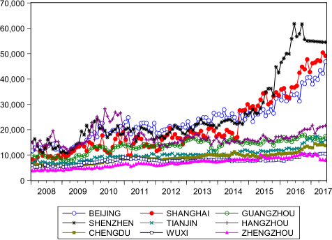
Figure 1: Residential real estate prices ($Yuan/m^{2}$) in China from Jan/2008 to Jun/2017. There is a significant rise in most Tier-1 cities, while prices of Tier-2 and Tier-3 cities had grown more moderately. Source: WIND Database

In order to gain an insight on the recent housing boom in China, one needs to trace back to the aftermath of 2007 Global Financial Crisis (GFC). In November 2008, the Chinese government had announced a 4-trillion investment package that aims to stimulate domestic economy. Despite a brief period of accelerating growth, the real sector had continued to slow down according to Fig. 2. The slowdown is particularly noticeable in the Li Keqiang index - an alternative measurement of macroeconomic performance. On the other hand, the credit sector had become increasingly lenient toward household borrowing. According to Fig. 3, we observe a rapid growth in medium-to-long-term household borrowing, with a steady decrease of interest rates (upper panel). There is also a dramatic rise in terms of the elasticity of Personal Housing Loan (PHL) relative to GDP, as well as the proportion of PHL relative to the total amount of loans in the Big-4 Chinese banks (lower panel). The traditional cultural urge to hold real estate, accompanied by a lack of alternative investment channels since the stock market crash in 2008 and 2015, had prompted households to participate even more aggressively in the spending spree over housing while giving banks further incentives to lend to households. The increasing level of financial fragility associated with the over-heating housing market had raised concerns of the central government. In the official newspaper People’s daily (Ren Min Ri Bao), the potential danger of a real estate bust was, for the first time, referred to as a “grey rhino”, alluding to extreme events in large probability instead of a lower-probability Talebic “black swan” (Taleb, 2007). A series of purchasing restrictions was issued as early as 2010 in order to curb the over-heating market. Lugovskyy et al. (2014) conduct an experimental study on the efficacy of such asset holding caps and argue that such policy would be effective in eliminating bubbles if it is properly designed.

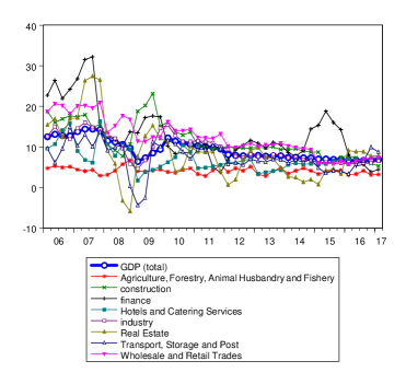
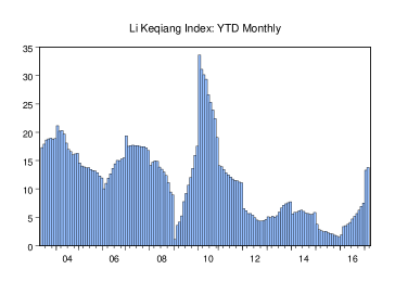
Figure 2: Top panel: Growth rate of GDP as a function time from 2005 to 2017; bottom panel: Li Keqiang index as defined in footnote 2. The GDP growth had steadily fallen over the decade, accompanied by similar downward trends in most sub-sectors. The finance sector had boomed over a brief period since 2014, followed by a sharp decrease in mid-2015 due to the stock market crash over that period. See Jiang et al. (2010) for detailed analysis over the stock market crash. Source: WIND Database

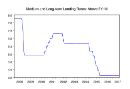
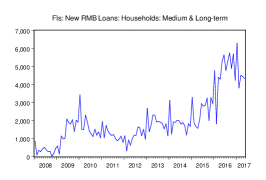
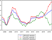
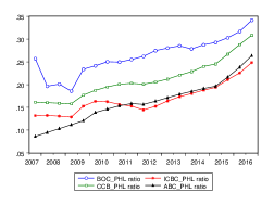
Figure 3: Top-left panel: Provident Fund Interest Rate as a function of time. Top-right panel: Stock of New Medium & Long-Term RMB loans to Households (CNY 100mn) Bottom-left panel: Elasticity of Personal Housing Loan (PHL), Real Estate Development Loan (RED), and Commercial Real-estate Loan (CRE) relative to GDP. Bottom-right panel: Proportion of Personal Housing Loan (PHL) over total assets in Big-4 Banks

Unlike other breeds of speculative bubbles, the burst of a real-estate bubble could potentially engender far-reaching consequence due to the deep involvement of banking sector. Historically, the burst of Japanese real-estate bubble in the late 1980s had led the country into a decades-long recession that hasn’t yet recovered to date. The full ramification of the latest sub-prime mortgage crisis in the US and the subsequent global contagion is still yet to be seen. In order to avoid systemic financial crisis and the ensuing economic depression, it is vital to conduct ex-ante bubble diagnosis and provide well-informed policy guidance that aims to curb bubbles at its formative stage prior to the critical point.

As is pointed out by Case and Shiller (2003), the term “bubble” is widely used but rarely clearly defined. Amongst existing studies, bubble is commonly referred to as a temporary deviation of price from its fundamental value. There are generally two strands of literature in the study of housing bubbles from such a fundamental approach. The first strand applies the idea of user-cost model of Poterba (1984), which usually takes housing rent as a proxy of future cash flows and derives the equilibrium price of real estates based on non-arbitrage condition and efficient market hypothesis (Gallin, 2006; Hoffmann et al., 2012). The second strand studies the long-term relationship between housing prices and the underlying economic fundamentals. A cointegration model is generally applied and bubble is identified if there is no cointegration between housing prices and fundamental factors (Hui and Yue, 2006; Mikhed and Zemcik, 2007; Arshanapalli and Nelson, 2008).

Yet the fundamental definition of bubble does not capture the inherent non-linear dynamics of bubble formation process that drives the bubble. From a Minskyan point of view, bubbles are inherently unstable due to bounded rationality of investors (Minsky, 1975). Kindleberger (1989) anatomized a typical financial bubble in five distinct phases: displacement, credit expansion, euphoria, overtrading, and revulsion. Hence, in addition to the fundamental definition of bubbles, we cannot overlook the speculative nature of a bubble driven by herd behaviour and aggravated by drastic credit expansion and self-reinforcing positive feedback mechanism. Such unsustainable price trajectory is often characterized by a faster-than-exponential growth in asset price during the bubble formation process prior to its burst. This is mathematically formalized by Sornette (2003) in the development of Log-Periodic-Power-Law-Singularity (LPPLS) model. The LPPLS framework had made a remarkable track record in early diagnosis of bubbles as well as post-mortem analysis of historical bubbles. Sornette and Zhou (2004) studies the 2000 new economy bubble. Zhou and Sornette (2006) examines the US Real-Estate Bubble. Jiang et al. (2010) conducted a bubble diagnosis of 2005-2007 and 2008-2009 Chinese stock market bubbles. More recently, Zhang et al. (2017) investigate the critical transitions of Chinese real estate bubbles based on the LPPLS framework. From a laboratory setting, Himmelberg et al. (2005) conduct a controlled price formation experiment, which detects the existence of super-exponential bubble due to positive feedback.

This paper aims to conduct a series of bubble diagnostic analysis over nine representative Chinese cities from two aspects. First, we investigate whether the prices had been significantly deviating from economic fundamentals by applying a standard Engle-Granger cointegration test. Second, we apply the Log-Periodic-Power-Law-Singularity (LPPLS) model to detect whether there is any evidence of unsustainable, self-reinforcing speculative behaviours amongst the univariate price series. We differ from Zhang et al. (2017) in two aspects. First, a conventional cointegration analysis is incorporated in comparison to the LPPLS analysis. Second, we focus on diagnosing the LPPLS signals based on the filter condition instead of the critical time ($t_{c}$). On the policy side, we argue that it is vital to conduct bubble diagnostic test in order to identify whether bubbles are fundamental-driven or speculative-driven, and design policies that address the specific bubble signatures.

The rest of the paper is organized as follows. Section 2 outlines the methodological framework of bubble diagnosis from both fundamental and LPPLS perspectives. Section 3 describes the data and defines the variables used in this study. Section 4 provides the empirical results. Finally, section 5 concludes.

2 Methodology

2.1 The Fundamental Diagnosis of Bubbles: Pairwise Engle-Granger Approach

We apply a simple pairwise cointegration model of Engle and Granger (1987) to investigate whether there is any long-run relationship between housing prices and its corresponding fundamental factors. Suppose there are two non-stationary series $X_{t}$ and $Y_{t}$ that are integrated of order one $I(1)$. If certain linear combination of $X_{t}$ and $Y_{t}$ yields I(0), then we say that $X_{t}$ and $Y_{t}$ are cointegrated. The Engle-Granger cointegration test is simply done in two steps: first, we conduct the Augmented Dicky-Fuller (ADF) test to see if all series are $I(1)$. Second, we run a simple OLS regression of $Y_{t}=\beta_{0}+\beta_{1}t+\beta_{2}X_{t}+u_{t}$ and test if $u_{t}$ is $I(0)$. In the context of this paper, a fundamental bubble exists if (i) the price series are not $I(0)$, and (ii) the fundamental factors are $I(0)$, or the $I(1)$ fundamental factor is not cointegrated with $I(1)$ price series.

2.2 The Log-Periodic-Power-Law-Singularity (LPPLS) Diagnosis of Bubbles

We further apply the LPPLS framework proposed by Sornette (2003) in order to examine whether the housing prices contain any sign of unsustainable speculative component characterized by faster-than-exponential growth pattern due to herd-behaviour and positive feedback mechanism, coupled with a periodic oscillation dynamics due to heterogeneous interactions between fundamentalists and trend chasers. Hence we apply the Johansen-Ledoit-Sornette (JLS) model, of which the law of motion takes the following form:

$$\frac{dp}{p}=\mu(t)dt+\sigma(t)dW-\kappa dj,$$ (1)

where $\mu(t)$ is the drift and $\sigma(t)$ is the diffusion component of a standard Wiener process augmented by a discontinuous jump $dj$ with the dummy switch $j=0$ prior to the critical time and $j=1$ after the crash. We further define the crash hazard rate $h(t)$, which is proportional to the expectation of $dj$: $h(t)=E[dj]/dt$. By applying the rational expectation condition of Blanchard and Watson (1982), we obtain

$$\mu(t)=\kappa h(t).$$ (2)

According to Sornette (2003), the hazard rate takes the following form:

$$h(t)=\alpha(t_{c}-t)^{m-1}(1+\beta cos(\omega\ln(t_{c}-t)-\phi^{\prime}),$$ (3)

Eq. (3) consists of a component of power law singularity due to self-reinforcing herd behaviour of noise traders $\alpha(t_{c}-t)^{m-1}$, as well as an oscillating component $\beta\cos(\omega\ln(t_{c}-t)-\psi^{\prime})$ driven by the heterogeneous interactions between fundamentalists and trend chasers. The power-law singularity captures the positive feedback mechanism driven by the self-reinforcing beliefs while the log-periodicity embodies the tug-of-war between the two types of investors leading to large scale volatility leading to the singularity, or critical time ($t_{c}$). Combining (1 - 3) yields

$$E[lnp(t)]=A+B(t_{c}-t)^{m}+C(t_{c}-t)^{m}\cos[\omega\ln(t_{c}-t)-\phi],$$ (4)

with $B=-\kappa\alpha/m$ and $C=-\kappa\alpha\beta/\sqrt{m^{2}+\omega^{2}}$. Generally, the bubble regimes are conditioned by $0<m<1$ and $B<0$, where $m<1$ insures the singularity - the expected log-price diverges at $t_{c}$ and the two conditions combined insure that the price grows super-exponentially towards the critical time $t_{c}$.

Given its non-linear structure, the conventional method of calibrating Equation (4) follows a two-step process. The first step involves a taboo search of Cvijovic and Klinowski (1995) to find N number of candidate solutions from our given search space. Each of these solutions is used as an initial estimates in a Levenberg-Marquardt non-linear least squares algorithm. We take the solution with the minimum sum of squares of the residuals. This paper adopts the procedure proposed by Filimonov and Sornette (2013) and Sornette et al. (2015) where the number of non-linear parameters has been reduced to just 3: $t_{c}$, $m$, $\omega$ for parsimonious purpose. The filter condition is given by Sornette et al. (2015) below:

$$0.01 \leq m\leq 0.99$$ (5)

$$2 \leq \omega\leq 25$$ (6)

$$t_{2}-0.05dt \leq t_{c}\leq t_{2}+0.1dt$$ (7)

$$2.5 \leq \frac{\omega}{2\pi}\ln[\frac{t_{c}-t_{1}}{t_{c}-t_{2}}]$$ (8)

$$1 \leq |mB/\omega C|$$ (9)

In the context of this paper, if all filter conditions above are met, we define a bubble in the corresponding series. We set the start time at $t_{1}=200801$, then move forward on a monthly basis until $t_{1}=201010$. The end time $t_{2}$ fixed at $t_{2}=201705$.

3 Data Description

Our data is collected from WIND and National Bureau of Statistic from Jan-2008 to Jun-2017 on a monthly basis. We have chosen nine representative cities, which include the four Tier-1 cities, as well as five Tier 2&3 cities: Beijing, Shanghai, Guangzhou, Shenzhen, Tianjin, Hangzhou, Chengdu, Wuxi, and Zhengzhou. We take the average price of traded residential building ($Yuan/m^{2}$) as a proxy for housing market condition ($P_{city}$). In addition, regional GDP ($GDP_{city}$), disposable income of urban residents ($INC_{city}$), and urban population of the respective cities ($POP_{city}$) are chosen as a measurement of fundamentals. Furthermore, in order to analyse how credit factors influences the housing price dynamics, we take provident fund interest rate of individual housing loans ($IRH$), broad money ($M2$), as well as medium & long-term new RMB loans ($NRLH$) granted to households ($>5years$). The descriptive statistics of housing prices for Tier-1 cities and the representative Tier-2&3 cities are presented in Table 1 and Table 2.

Table 1: Descriptive statistics of residential housing prices ($Yuan/m^{2}$) in Tier-1 cities: Jan/2008-Jun/2017. Source: WIND Database

Price Statistic	Beijing	Shanghai	Guangzhou	Shenzhen
Mean	23234.07	21165.75	13604.13	25953.03
Median	22323.50	17089.00	13916.00	20865.00
Maximum	46834.00	50401.00	17882.00	61756.00
Minimum	10486.38	7510.870	7977.821	10770.00

Table 2: Descriptive statistics of residential housing prices ($Yuan/m^{2}$) for 5 representative cities outside Tier-1 category: Jan/2008-Jun/2017 Source: WIND Database

Price Statistic	Tianjin	Hangzhou	Chengdu	Wuxi	Zhengzhou
Mean	10199.36	17012.28	8870.815	7729.790	6853.389
Median	9998.000	16289.50	8881.000	7853.558	6789.000
Maximum	17366.00	28214.00	14447.00	10591.94	10538.00
Minimum	6470.760	11382.54	5336.630	4668.800	3771.000

4 Results

4.1 Are housing prices deviating from economic fundamentals in the long run?

In this subsection, we examine whether housing prices are significantly derailed from the selected fundamental factors. We include three macro-variables on a regional basis, i.e. GDP, income per capita, and population of each representative cities. We first run a standard ADF test with constant and trend to examine whether the prices series and fundamental factors are stationary. If any price series is stationary, it indicates a self-correcting property in the series, hence no bubble. Table 3 reports the main result of our analysis. As for the price series, we found that all the prices are integrated of order 1 except Guangzhou. As for the macro-variables, we found that all the regional GDP series are non-stationary, yet for income per capita (INC) and population (POP), INC of Hangzhou, Wuxi, and Zhengzhou, as well as POP of Beijing and Wuxi are integrated of order zero ($I(0)$). We further conduct the Engle-Granger test to analyze whether the $I(1)$ price series are cointegrated with the $I(1)$ fundamentals. Generally, there are no clear sign of such cointegration except for Shanghai, where GDP is cointegrated with price at $5\%$ LOS and INC at $10\%$ LOS. Yet there is no evidence of cointegration between $P_{Shanghai}$ and $POP_{Shanghai}$. Overall, from this preliminary analysis, we conclude that only Guangzhou is excluded from the bubble hypothesis from the fundamental perspective.

Table 3: Engle-Granger diagnosis with fundamental factors. We denote residential housing price ($Yuan/m^{2}$) of city $x$ as $P_{x}$, per capita income of city $x$ as $INC_{x}$, and urban population of city $x$ as $POP_{x}$. It is found that $P_{Guangzhou}$, $POP_{Beijing}$, $INC_{Hangzhou}$, $INC_{Wuxi}$, $POP_{Wuxi}$, and $INC_{Zhengzhou}$ are $I(0)$ while the rest of variables $I(1)$. Guangzhou is excluded from the test since $P_{Guangzhou}$ is stationary. For other cities, a bubble exists since there is at least one fundamental factor that is not cointegrated with price series.

Cities	GDP	INC	POP
Beijing	-1.54091	-1.55562	N/A
	(0.8076)	(0.8021)	N/A
Shanghai	-3.64674	-3.26836	-1.73829
	$(0.0317)^{\star\star}$	$(0.0786)^{\star}$	(0.7256)
Guangzhou	N/A	N/A	N/A
	N/A	N/A	N/A
Shenzhen	-2.23465	-0.13013	-1.3957
	(0.4644)	(0.9936)	(0.8555)
Tianjin	-2.08396	-3.43469	-1.84866
	(0.547)	(0.0535)	(0.6721)
Hangzhou	-2.72684	N/A	-2.81171
	(0.2288)	N/A	(0.1973)
Chengdu	-1.39695	-1.48165	-1.32539
	(0.8552)	(0.8285)	(0.8749)
Wuxi	-0.91553	N/A	N/A
	(0.9489)	N/A	N/A
Zhengzhou	-2.59795	N/A	-3.06301
	(0.2824)	N/A	(0.1219)

4.2 Is there unsustainable speculation in the housing market?

As pointed out by Kindleberger (1989), the bounded rationality of investors plays a pivotal role in the formation of speculative bubble. Furthermore, the endogenous nature of credit expansion renders such leveraged speculation possible. Such unsustainable, self-reinforcing bubble is often associated with an inherent relationship between asset prices and the underlying financial factors, and characterized by a faster-than-exponential growth component of price series, which is mathematically formalized by Sornette (2003) in the development of Log-Periodic-Power-Law-Singularity (LPPLS) model.

We begin with investigating whether there is any long-run relationship between housing prices and the underlying credit factors in a similar pairwise cointegration model. Three financial variables are selected, i.e. new RMB loans to households over five-years term ($NRLH$), provident fund interest rates of households ($IRH$), and broad money ($M2$). From the ADF tests, we found that all the three factors are $I(1)$. We further conduct a EG test between housing prices and the three financial factors, as is shown in Table 4. The result is generally in line with Xu and Chen (2012). It is evident that bank lending to household is strongly associated with the long-term surge of housing prices amongst most cities, as reflected in the cointegration between $P_{x}$ and $NRLH$ in the sample. The relationship is relatively weaker in $M2$ and $IRH$.

Table 4: Pairwise Engle-Granger test for real estate prices against financial variables. We denote New RMB Loans for Households as $NRLH$, Interest Rate for Households as $IRH$, and Broad Money as $M2$. There is a long-run relationship between housing prices and the underlying credit factors in Beijing, Shanghai, Shenzhen, Tianjin, Hangzhou, and Zhengzhou. The evidence is particularly strong in terms of $NRLH$.

Cities	$NRLH$	$IRH$	$M2$
Beijing	$-2.782645$	$-1.261070$	$-1.400137$
	$(0.06501)^{\star}$	$(0.6443)$	$(0.9794)$
Shanghai	$-2.939178$	$-2.143475$	$-3.021259$
	$(0.0451)^{\star\star}$	$(0.2285)$	$(0.0369)^{\star\star}$
Guangzhou	$N/A$	$N/A$	$N/A$
	$N/A$	$N/A$	$N/A$
Shenzhen	$-4.528026$	$-2.242361$	$-1.891156$
	$(0.0004)^{\star\star\star}$	$(0.1932)$	$(0.3350)$
Tianjin	$-3.384025$	$-2.353078$	$-3.208008$
	$(0.0142)^{\star\star}$	$(0.1582)$	$(0.0229)^{\star\star}$
Hangzhou	$-3.275892$	$-3.241492$	$-2.762250$
	$(0.0191)^{\star\star}$	$(0.0210)^{\star\star}$	$(0.0681)^{\star}$
Chengdu	$-2.500844$	$-1.859283$	$-1.813710$
	$(0.1189)$	$(0.3499)$	$(0.3706)$
Wuxi	$-1.327366$	$-0.798439$	$-0.837302$
	$(0.6136)$	$(0.8143)$	$(0.8031)$
Zhengzhou	$-3.136173$	$-3.173356$	$-3.209019$
	$(0.0276)^{\star\star}$	$(0.0250)^{\star\star}$	$(0.0228)^{\star\star}$

Table 5: Occurrence of Log-Periodic-Power-Law-Singularity (LPPLS) Signals. There is evidence of LPPLS signatures in Shanghai, Shenzhen, Tianjin, and Chengdu.

	LPPLS Diagnosis	LPPLS Strength
Beijing	N	$0\%$
Shanghai	Y	$100\%$
Guangzhou	N	$0\%$
Shenzhen	Y	$5.89\%$
Tianjin	Y	$5.89\%$
Hangzhou	N	$0\%$
Chengdu	Y	$17.65\%$
Wuxi	N	$0\%$
Zhengzhou	N	$0\%$

We further apply the LPPLS framework to diagnose whether the housing prices contain faster-than-exponential components according to Jiang et al. (2010), as shown in Table 5. The LPPLS strength here is defined as the proportion of windows with LPPLS signature over the total number of windows. We found four cities that exhibit signs of faster-than-exponential growth component, i.e. Shanghai, Shenzhen, Tianjin, and Chengdu. The LPPLS strength is particularly strong in Shanghai, of which all time windows are diagnosed with positive LPPLS signals. Surprisingly, Chengdu has a moderate level of LPPLS signal, despite the absence of relationship between $P_{Chengdu}$ and the underlying financial factors. It indicates that the housing price in Chengdu is likely to be driven by non-financial speculative factors. Shenzhen and Tianjin had shared a similar degree of LPPLS strength, although the housing price in Shenzhen is much higher in absolute terms.

Overall, we conclude that amongst the nine cities being examined, only Guangzhou does not exhibit clear signs of bubble due to its stationary property and absence of LPPLS signature, as summarized in Table 6. The result is generally in line with Zhang et al. (2017), which diagnosed an imminent high risk of turning point or correction in Beijing, Tianjin and Chengdu in 2017 while Shanghai and Shenzhen are at high risk in 2018 in terms of the quantile-based DS-LPPLS Confidence indicator. Similarly, there is no evidence of bubble in Guangzhou according to this previous study.

Table 6: Summary of Results: Engle-Granger (EG) vs. Log-Periodic-Power-Law-Singularity (LPPLS) Diagnosis. Only Guangzhou does not exhibit a clear bubble signature amongst the nine cities being examined.

	EG	LPPLS	Overall
Beijing	Y	N	Y
Shanghai	Y	Y	Y
Guangzhou	N	N	N
Shenzhen	Y	Y	Y
Tianjin	Y	Y	Y
Hangzhou	Y	N	Y
Chengdu	Y	Y	Y
Wuxi	Y	N	Y
Zhengzhou	Y	N	Y

It is evident from the empirical analysis above that the purchase & credit restrictions enforced since April 2010 had by and large failed to curb excessive growth of housing prices, despite the strenuous effort of the central government. This is in contrast with Lugovskyy et al. (2014), which argues from a laboratory setting that such asset holding caps could be effective if it is well designed. Yet since 2017, the Chinese authority had announced another series of unconventional policies. In early 2017, a new policy named selling restriction (Xian-Mai) was implemented in 14 cities, which prohibits real estate buyers and investors to sell within a period of time that ranges from 2 years to 5 years. This policy had provided an efficient means to drive away short-term, speculative investors meanwhile preventing large-scale stampede from real estate markets that would eventually result in a crash. We recommend that, in order to design effective policy, it is vital to conduct bubble diagnostic test and implement relevant policies in cities with specific bubble signatures. For cities with significant LPPLS signature, it is vital to design policies that aim to eliminate excessive expectations on housing prices beyond mere demand-side control. For example, the selling constraint mentioned above would effectively eliminate the short-term speculative investors, thus stabilizing the price. Yet for cities that are diagnosed with fundamental bubbles without LPPLS signature, it would be more appropriate to design supply-side policies that accommodate the demand pressure arising from economic fundamentals.

5 Conclusion

The Chinese housing market had sustained a rapid growth since 2008, which is in stark contrast with the gloomy outlook of global economy and the steady decline of domestic real sector since the aftermath of 2007 GFC. It had raised concerns of both academics and policy makers alike.

This paper aims to provide an informed test over the bubble hypothesis of Chinese housing market based on nine representative cities. Our study differs from previous ones in the sense that we incorporate not only a conventional bubble definition from a fundamental perspective by means of a cointegration model, but also from a behavioural perspective of the emerging LPPLS framework to detect whether there is any unsustainable traits in the price dynamics characterized by faster-than-exponential growth signals. We found that amongst the nine cities being examined, only Guangzhou does not exhibit a clear sign of bubble.

On the policy side, we suggest that the conventional purchase & credit restrictions haven’t had the desired effect in curbing excessive increase of housing prices amongst the sample being examined. Given the heterogeneity that exists amongst cities with distinct bubble signatures, it is vital to conduct bubble diagnostic tests and implement relevant policies toward the specific bubble characteristics, rather than enforcing one-that-fits-for-all type policy that does not take into account such heterogeneity. We propose that, for cities with significant LPPLS signature, it is vital to implement policies that aim to eliminate speculative demand. In cities without LPPLS signature, the supply-side policies would be more appropriate in addressing the pressure arising from fundamental demand. The implications of such bubble diagnostic test toward a wider range of cities, as well as the efficacy of current policies will be further investigated in future research.

Acknowledgements
This research is supported by National Natural Science Foundation of China (No. 71721001, 71231008 & 71671191) and Young Academic Mentorship Project of Sun Yat-sen University (No. 14000-31610161). We are grateful for the generous comments and suggestions from participants at International Conference on Econophysics (ICE) 2017 Shanghai, Computational Economics and Finance Conference (CEF) 2017 New York, and Artificial Economics Conference (AE) 2017 Tianjin. The usual disclaimer applies.

Reference

Appendix: Selected LPPLS outputs for cities with positive signals.

Table 7: LPPLS Output: Shanghai

t1	tc	m	w	A	B	C	Bm/Cw	$Ind_{LPPLS}$
200801	201705	0.746	4.245	10.883	-0.004	0.001	1.438	1
200802	201705	0.74	4.247	10.89	-0.005	0.001	1.45	1
200803	201705	0.713	4.251	10.923	-0.006	0.001	1.51	1
200804	201705	0.712	4.247	10.923	-0.006	0.001	1.513	1
200805	201705	0.747	4.267	10.883	-0.004	0.001	1.43	1
200806	201705	0.75	4.289	10.882	-0.004	0.001	1.412	1
200807	201705	0.776	4.393	10.867	-0.004	0	1.317	1
200808	201705	0.779	4.402	10.866	-0.003	0	1.309	1
200809	201705	0.781	4.408	10.865	-0.003	0	1.303	1
200810	201705	0.775	4.384	10.868	-0.004	0	1.323	1
200811	201705	0.765	4.332	10.872	-0.004	0.001	1.356	1
200812	201705	0.763	4.316	10.873	-0.004	0.001	1.365	1
200901	201705	0.751	4.228	10.879	-0.004	0.001	1.408	1
200902	201705	0.748	4.186	10.88	-0.004	0.001	1.424	1
200903	201705	0.716	4.086	10.912	-0.006	0.001	1.484	1
200904	201705	0.708	3.947	10.912	-0.006	0.001	1.511	1
200905	201705	0.703	3.839	10.911	-0.006	0.001	1.523	1
200906	201705	0.7	3.77	10.91	-0.006	0.001	1.526	1
200907	201705	0.702	3.824	10.911	-0.006	0.001	1.525	1
200908	201705	0.707	3.913	10.912	-0.006	0.001	1.523	1
200909	201705	0.715	4.07	10.913	-0.006	0.001	1.515	1
200910	201705	0.721	4.159	10.913	-0.005	0.001	1.508	1
200911	201705	0.715	4.067	10.913	-0.006	0.001	1.513	1
200912	201705	0.751	4.263	10.882	-0.004	0.001	1.477	1
201001	201705	0.762	4.429	10.88	-0.004	0	1.454	1
201002	201705	0.768	4.482	10.878	-0.004	0	1.443	1
201003	201705	0.767	4.468	10.878	-0.004	0	1.445	1
201004	201705	0.774	4.553	10.877	-0.004	0	1.435	1
201005	201705	0.806	4.878	10.868	-0.003	0	1.365	1
201006	201705	0.805	4.867	10.869	-0.003	0	1.368	1
201007	201705	0.793	4.756	10.872	-0.003	0	1.389	1
201008	201705	0.768	4.499	10.877	-0.004	0	1.393	1
201009	201705	0.763	4.447	10.878	-0.004	0	1.386	1
201010	201705	0.785	4.669	10.874	-0.003	0	1.413	1

Table 8: LPPLS Output: Shenzhen

t1	tc	m	w	A	B	C	Bm/Cw	$Ind_{LPPLS}$
200801	201709	0.799	3.172	11.224	-0.003	0.001	1.054	1
200802	201709	0.879	3.142	11.172	-0.002	0	1.038	1
200803	201709	1	3.089	11.112	-0.001	0	1.024	0
200804	201709	1	3.126	11.114	-0.001	0	1.011	0
200805	201709	1	3.136	11.115	-0.001	0	1.007	0
200806	201709	1	3.126	11.114	-0.001	0	1.011	0
200807	201709	1	3.138	11.115	-0.001	0	1.007	0
200808	201709	1	3.196	11.118	-0.001	0	0.988	0
200809	201709	1	3.232	11.12	-0.001	0	0.977	0
200810	201709	1	3.237	11.121	-0.001	0	0.975	0
200811	201709	1	3.241	11.121	-0.001	0	0.974	0
200812	201709	1	3.254	11.122	-0.001	0	0.971	0
200901	201709	1	3.215	11.119	-0.001	0	0.98	0
200902	201709	1	3.173	11.116	-0.001	0	0.99	0
200903	201709	1	3.098	11.111	-0.001	0	1.003	0
200904	201708	1	2.946	11.097	-0.001	0	1.019	0
200905	201707	1	2.769	11.078	-0.001	0	1.032	0
200906	201707	0	2.192	166070.8	-166058	0.262	0.626	0
200907	201707	0	2.233	155980.8	-155968	0.265	0.608	0
200908	201707	0	2.261	151409.9	-151397	0.27	0.588	0
200909	201707	0	2.265	217427	-217414	0.271	0.585	0
200910	201707	0	2.276	72515.84	-72503	0.273	0.578	0
200911	201707	0	2.27	118581.4	-118569	0.272	0.581	0
200912	201707	0	2.275	100781.6	-100769	0.273	0.579	0
201001	201707	0	2.267	189005.6	-188993	0.272	0.582	0
201002	201707	0	2.243	118439.3	-118426	0.271	0.588	0
201003	201707	0	2.203	188795.2	-188782	0.27	0.595	0
201004	201707	0	2.192	105828.1	-105815	0.27	0.596	0
201005	201707	0	2.178	132157.1	-132144	0.27	0.597	0
201006	201707	0	2.174	176746.1	-176733	0.27	0.597	0
201007	201707	0	2.213	255119.7	-255107	0.269	0.596	0
201008	201707	0	2.233	162061.7	-162049	0.269	0.594	0
201009	201707	0	2.235	300033.9	-300021	0.269	0.594	0
201010	201707	0	2.225	125547.9	-125535	0.269	0.595	0

Table 9: LPPLS Output: Tianjin

t1	tc	m	w	A	B	C	Bm/Cw	$Ind_{LPPLS}$
200801	201706	0.659	2.227	9.797	-0.005	0.001	1.29	1
200802	201706	0.71	2.121	9.777	-0.004	0.001	1.292	1
200803	201705	0.801	1.953	9.753	-0.002	0.001	1.296	0
200804	201705	0.991	1.658	9.727	-0.001	0	1.327	0
200805	201705	1	1.677	9.727	0	0	1.309	0
200806	201705	1	1.727	9.728	0	0	1.278	0
200807	201705	1	1.769	9.729	0	0	1.254	0
200808	201705	1	1.789	9.729	0	0	1.244	0
200809	201705	1	1.815	9.73	0	0	1.23	0
200810	201705	1	1.833	9.731	0	0	1.221	0
200811	201705	1	1.82	9.73	0	0	1.228	0
200812	201705	1	1.81	9.73	0	0	1.232	0
200901	201705	1	1.815	9.73	0	0	1.23	0
200902	201705	1	1.815	9.73	0	0	1.23	0
200903	201705	1	1.787	9.729	0	0	1.244	0
200904	201705	1	1.738	9.728	0	0	1.269	0
200905	201705	1	1.686	9.728	0	0	1.296	0
200906	201705	1	1.641	9.727	0	0	1.321	0
200907	201705	1	1.567	9.726	0	0	1.363	0
200908	201705	1	1.55	9.726	0	0	1.373	0
200909	201705	1	1.523	9.726	0	0	1.388	0
200910	201705	0.882	1.633	9.736	-0.001	0	1.389	0
200911	201705	0.816	1.69	9.744	-0.002	0.001	1.404	0
200912	201705	0.719	1.767	9.761	-0.003	0.001	1.45	0
201001	201705	0.663	1.798	9.775	-0.005	0.001	1.492	0
201002	201705	0.681	1.793	9.77	-0.004	0.001	1.476	0
201003	201705	0.679	1.793	9.771	-0.004	0.001	1.479	0
201004	201705	0.707	1.783	9.764	-0.004	0.001	1.456	0
201005	201705	0.762	1.754	9.753	-0.002	0.001	1.423	0
201006	201705	0	0.698	47912.66	-47903	0.237	0.203	0
201007	201705	0	0.71	46551.48	-46541.9	0.239	0.183	0
201008	201705	0	0.708	23253.06	-23243.4	0.239	0.186	0
201009	201705	0	0.712	13937.11	-13927.5	0.239	0.18	0
201010	201705	0.759	1.776	9.755	-0.002	0.001	1.422	0

Table 10: LPPLS Output: Chengdu

t1	tc	m	w	A	B	C	Bm/Cw	$Ind_{LPPLS}$
200801	201709	0.92	10.553	9.483	0	0	0.419	0
200802	201709	0.926	10.491	9.482	0	0	0.429	0
200803	201706	0.61	2.451	9.648	-0.007	0.002	1.036	1
200804	201705	0.68	2.261	9.62	-0.004	0.001	1.081	1
200805	201705	0.757	2.077	9.599	-0.002	0.001	1.126	1
200806	201705	0.864	1.832	9.578	-0.001	0	1.189	0
200807	201705	0.916	1.737	9.575	-0.001	0	1.218	0
200808	201705	0.981	1.623	9.574	-0.001	0	1.259	0
200809	201705	1	1.604	9.575	-0.001	0	1.258	0
200810	201705	1	1.625	9.576	-0.001	0	1.237	0
200811	201705	1	1.642	9.577	-0.001	0	1.221	0
200812	201705	1	1.652	9.577	-0.001	0	1.211	0
200901	201705	1	1.658	9.577	-0.001	0	1.206	0
200902	201705	1	1.659	9.577	-0.001	0	1.206	0
200903	201705	1	1.65	9.577	-0.001	0	1.213	0
200904	201705	1	1.636	9.577	-0.001	0	1.225	0
200905	201705	1	1.617	9.576	-0.001	0	1.241	0
200906	201705	1	1.59	9.576	-0.001	0	1.262	0
200907	201705	1	1.567	9.576	-0.001	0	1.28	0
200908	201705	1	1.553	9.576	-0.001	0	1.291	0
200909	201705	0.953	1.603	9.576	-0.001	0	1.282	0
200910	201705	0.855	1.75	9.58	-0.001	0.001	1.246	0
200911	201705	0.699	2.033	9.61	-0.004	0.001	1.196	1
200912	201706	0.532	2.359	9.674	-0.013	0.003	1.152	1
201001	201706	0.333	2.798	9.871	-0.07	0.008	1.085	1
201002	201707	0.147	3.258	10.598	-0.512	0.023	1.007	1
201003	201708	0.024	3.602	17.37	-6.913	0.049	0.955	0
201004	201708	0	3.638	137541.3	-137531	0.055	0.965	0
201005	201708	0	3.611	67216.53	-67206	0.053	0.993	0
201006	201708	0	3.6	94994.89	-94984.4	0.051	1.01	0
201007	201708	0	3.576	309174.8	-309164	0.049	1.047	0
201008	201707	0	3.558	63710.24	-63699.8	0.047	1.079	0
201009	201705	0.077	7.497	11.155	-1.157	0.029	0.406	0
201010	201705	0.065	7.534	11.471	-1.453	0.033	0.384	0

References

- Ahuja et al. (2010) Ahuja, A., Cheung, L., Han, G., Porter, N., Zhang, W., 2010. Are house prices rising too fast in china. Working paper 08/2010, Hong Kong Monetary Authority.
- Arshanapalli and Nelson (2008) Arshanapalli, B., Nelson, W., 2008. A Cointegration Test to Verify the Housing Bubble. The International Journal of Business and Finance Research 2 (2), 35–43.
- Case and Shiller (2003) Case, K. E., Shiller, R. J., 2003. Is There a Bubble in the Housing Market? Brookings Papers on Economic Activity 34 (2), 299–362.
- Dickey and Fuller (1979) Dickey, D. A., Fuller, W. A., 1979. Distribution of the estimators for autoregressive time series with a unit root. Journal of the American Statistical Association 74 (366), 427–431.
- Economist (2010) Economist, 2010. Keqiang ker-ching: How china’s next prime minister keeps tabs on its economy. Tech. rep.
-
Engle and Granger (1987)
Engle, R. F., Granger, C. W. J., March 1987. Co-integration and Error
Correction: Representation, Estimation, and Testing. Econometrica 55 (2),
251–276.
URL https://ideas.repec.org/a/ecm/emetrp/v55y1987i2p251-76.html -
Gallin (2006)
Gallin, J., 09 2006. The Long-Run Relationship between House Prices and
Income: Evidence from Local Housing Markets. Real Estate Economics 34 (3),
417–438.
URL https://ideas.repec.org/a/bla/reesec/v34y2006i3p417-438.html - Himmelberg et al. (2005) Himmelberg, C. P., Mayer, C. J., Sinai, T., 2005. Assessing high house prices: bubbles, fundamentals, and misperceptions. Tech. rep.
-
Hoffmann et al. (2012)
Hoffmann, M., Krause, M. U., Laubach, T., 2012. Trend growth expectations and
U.S. house prices before and after the crisis. Journal of Economic Behavior
& Organization 83 (3), 394–409.
URL https://ideas.repec.org/a/eee/jeborg/v83y2012i3p394-409.html - Hui and Yue (2006) Hui, E. C. M., Yue, S., 2006. Housing Price Bubbles in Hong Kong, Beijing and Shanghai: A Comparative Study. Journal of Real Estate Finance and Economics 33 (4), 299–327.
- Jiang et al. (2010) Jiang, Z.-Q., Zhou, W.-X., Sornette, D., Woodard, R., Bastiaensen, K., Cauwels, P., June 2010. Bubble diagnosis and prediction of the 2005-2007 and 2008-2009 Chinese stock market bubbles. Journal of Economic Behavior & Organization 74 (3), 149–162.
- Kindleberger (1989) Kindleberger, C., 1989. Manias, Panics, and Crashes: a history of financial crises. Palgrave Macmillan, New York.
- Lugovskyy et al. (2014) Lugovskyy, V., Puzzello, D., Tucker, S., Williams, A., 2014. Asset-holdings caps and bubbles in experimental asset markets. Journal of Economic Behavior & Organization 107 (PB), 781–797.
-
Mikhed and Zemcik (2007)
Mikhed, V., Zemcik, P., Oct. 2007. Testing for Bubbles in Housing Markets: A
Panel Data Approach. CERGE-EI Working Papers wp338, The Center for Economic
Research and Graduate Education - Economics Institute, Prague.
URL https://ideas.repec.org/p/cer/papers/wp338.html - Minsky (1975) Minsky, H., 1975. John Maynard Keynes. Columbia University Press, New York.
- Poterba (1984) Poterba, J., 1984. Tax subsidies to owner-occupied housing: An asset market approach. Quarterly Journal of Economics 99 (4), 729–752,.
- Sornette (2003) Sornette, D., 2003. Why Stock Markets Crash: Critical Events in Complex Financial Systems. Princeton University Press, New Jersey.
- Sornette and Zhou (2004) Sornette, D., Zhou, W.-X., 2004. Evidence of fueling of the 2000 new economy bubble by foreign capital inflow: implications for the future of the US economy and its stock market. Physica A: Statistical Mechanics and its Applications 332 (C), 412–440.
- Taleb (2007) Taleb, N. N., 2007. The Black Swan: The Impact of the Highly Improbable. Random House, New York.
- Wucker (2016) Wucker, M., 2016. The Gray Rhino: How to Recognize and Act on the Obvious Dangers We Ignore. St. Martin’s Press, New York.
- Xu and Chen (2012) Xu, X. E., Chen, T., January 2012. The effect of monetary policy on real estate price growth in China. Pacific-Basin Finance Journal 20 (1), 62–77.
- Zhang et al. (2017) Zhang, Q., Sornette, D., Zhang, H., 2017. Anticipating critical transitions of Chinese housing markets. Swiss finance institute research paper no. 17-18.
- Zhou and Sornette (2006) Zhou, W.-X., Sornette, D., 2006. Is there a real-estate bubble in the US? Physica A: Statistical Mechanics and its Applications 361 (1), 297–308.