Byeon, Van Hentenryck, Bent, and Nagarajan

Communication-Constrained Expansion Planning

Communication-Constrained Expansion Planning
for Resilient Distribution Systems

Geunyeong Byeon and Pascal Van Hentenryck Industrial and Operations Engineering, University of Michigan Russell Bent and Harsha Nagarajan Los Alamos National Laboratory

Distributed generation and remotely controlled switches have emerged as important technologies to improve the resiliency of distribution grids against extreme weather-related disturbances. Therefore it becomes important to study how best to place them on the grid in order to meet a resiliency criteria, while minimizing costs and capturing their dependencies on the associated communication systems that sustains their distributed operations. This paper introduces the Optimal Resilient Design Problem for Distribution and Communication Systems (ORDPDC) to address this need. The ORDPDC is formulated as a two-stage stochastic mixed-integer program that captures the physical laws of distribution systems, the communication connectivity of the smart grid components, and a set of scenarios which specifies which components are affected by potential disasters. The paper proposes an exact branch-and-price algorithm for the ORDPDC which features a strong lower bound and a variety of acceleration schemes to address degeneracy. The ORDPDC model and branch-and-price algorithm were evaluated on a variety of test cases with varying disaster intensities and network topologies. The results demonstrate the significant impact of the network topologies on the expansion plans and costs, as well as the computational benefits of the proposed approach.

Planning for Resiliency, Power Systems, Branch and Price

1 Introduction

The last decades have highlighted the vulnerability of the current electric power system to weather-related extreme events. Between 2007 and 2016, outages caused by natural hazards, such as thunderstorms, tornadoes, and hurricanes, amounted to 90 percent of major electric disturbances, each affecting at least 50,000 customers (derived from Form OE-417 of U.S. DOE). It is also estimated that 90 percent of all outages occur along distribution systems (Executive Office of the President 2013). Moreover, the number of weather-related outages is expected to rise as climate change increases the frequency and intensity of extreme weather events (Executive Office of the President 2013). Accordingly, it is critical to understand how to harden and modernize distribution grids to prepare for potential natural disasters.

Distributed Generation (DG) is one of the advanced technologies that can be utilized to enhance grid resilience. DG refers to electric power generation and storage performed by a collection of distributed energy resources (DER). DG decentralizes the electric power distribution by supplying power to the loads closer to where it is located. The potential of DGs is realized via a system approach that views DGs and associated loads as a microgrid (Lasseter et al. 2002). A microgrid is often defined as a small-scale power system on medium- or low- voltage distribution feeder that includes loads and DG units, together with an appropriate management and control scheme supported by a communication infrastructure (Resende et al. 2011). When faults occur in the main grid, microgrids can be detached from the main grid and act in island mode to serve critical loads by utilizing local DGs or work in the grid-connected mode to provide ancillary services for the bulk system restoration (Wang et al. 2016a). Remotely controlled switches (RCS), another advanced technology, can be used to increase the grid flexibility by controlling the grid topology through a communication network and facilitate microgrid formations in emergencies. Other than the aforementioned operational enhancement measures, a grid can also be hardened physically by installing underground cables and/or upgrading the overhead lines with stronger materials, which reduces the physical impact of catastrophic events (Panteli et al. 2017).

A critical issue in building resilient distribution grids is to determine where to place such advanced devices (i.e., DGs, RCSs, and underground cables) and which existing lines to harden. It is also important to understand the dependency between the distribution grid and its associated communication network, which is critical to the effective operation of a modernized grid during emergency situations and is also vulnerable to extreme events (Falahati et al. 2012, Gholami et al. 2016, Martins et al. 2017, Li et al. 2017).

To address this pivotal and pressing issue, this paper introduces the Optimal Resilient Design Problem for Distribution and Communication Systems (ORPDDC). The ORDPDC determines how to harden and modernize an interdependent network to ensure its resilience against extreme weather events. Like recent papers (e.g., Yamangil et al. (2015), Barnes et al. (2017), the ORDPDC takes into account a set of disaster scenarios, each defining a set of power system components that are damaged during an extreme event. These scenarios are generated from historical data or probabilistic models of how power system components respond to hazard-specific stress (e.g., wind speed and flood depth). The ORDPDC considers the following upgrade options: a set of hardening options on existing power lines and communication links and a set of new components that can be added to the system—new lines, new communication pathways, remotely controlled switches, and distributed generation. The objective of the ORDPDC is to find the cheapest set of upgrade options that can be placed on the grid in order to guarantee that a minimal amount of critical and non-critical load be served in each scenario. These guarantees are called the reslience criteria.

The ORDPDC is modeled with a two-stage stochastic mixed integer program. The first stage decides an upgrade profile and the second stage decides how to utilize the DGs, RCSs, and power lines/communication links, whose availability is decided in the first-stage, to restore critical loads up to resiliency criteria (e.g., 98 %) in each disaster scenario. For each scenario, the second stage is viewed as a restoration model that identifies how to reconfigure the grid. Within this second stage problem, the physics of power flows is modeled with the steady-state, unbalanced three phase AC power equations and constraints that ensure that the radial structure of distribution grids is maintained. When the grid is reconfigured due to some disturbances, each island or microgrid must be connected to at least one control center that coordinates its DGs and loads and operates its RCSs. This communication requirement is modeled with a single-commodity flow model.

Several solution methods can be used to solve the ORDPDC, taking advantage of its block diagonal structure. Yamangil et al. (2015) proposed a Scenario-Based Decomposition (SBD) that restricts attention to a smaller set of scenarios and adds new ones on an as needed basis (see Section 5). However, in the worst case, SBD must solve the large-scale ORDPDC as a whole. Branch and Price (B&P), which combines column generation and branch-and-bound, is another solution method for approaching large-scale mixed-integer programming (Lübbecke and Desrosiers 2005). Although widely successful on many applications, it may suffer from degeneracy and long-tail effects as problems become larger. To address these difficulties, several stabilization techniques have been proposed and proven to be effective in many applications (e.g., (Du Merle et al. 1999, Oukil et al. 2007, Amor et al. 2009)). Nevertheless, the high degree of degeneracy and the significant scale of the ORDPDC create significant challenges for dual stabilization techniques.

To address these computational challenges, this paper proposes a B&P algorithm that systematically exploits the structure of the ORDPDC. The algorithm starts with a compact reformulation that results in strong lower bounds on the test cases and pricing subproblems that are naturally solved in parallel. Moreover, the B&P algorithm tackles the degeneracy inherent in the ORDPDC through a variety of acceleration schemes for the pricing subproblems: A pessimistic reduced cost, an optimality cut, and a lexicographic objective. The resulting B&P algorithm produces significant computational improvements compared to existing approaches.

The key contributions of this paper can be summarized as follows:

The paper proposes the first planning model for resilient distribution networks that combines the use of advanced technologies (e.g., DGs, RCSs, and undergrounding) with traditional hardening options and captures the dependencies between the distribution grid and its associated communication system.

The paper proposes an exact B&P algorithm for solving the ORDPDC problem, which systematically exploits the ORDPDC structure to obtain strong lower bounds and address its significant degeneracy issues.

The paper evaluates the impact of grid and communication system topologies on potential expansion plans. It also reports extensive computational results demonstrating the benefits of the proposed B&P algorithm on the test cases.

The remainder of this paper is organized as follows. Section 2 reviews related work on the ORDPDC. Section 3 formalizes the ORDPDC and Section 4 presents a tight linear approximation. Section 5 briefly reviews the SBD algorithm. Section 6 presents the new B&P algorithm. Section 7 describes the test cases. Lastly, Section 8 analyzes the behavior of the model on the case studies and Section 9 reports on the computational performance of the proposed algorithm. Section 10 concludes the paper.

2 Literature Review

There has been a considerable progress in advancing methods that address weather-related issues at distribution level (Wang et al. 2016a). Many studies develop post-fault distribution system restoration (DSR) models to bring power back as soon as possible and restore critical loads after a severe outage. Recently, DGs, RCSs, and redundant lines were utilized to leverage microgrids in load restoration. Most of the studies assume the existence of those devices beforehand (Chen et al. 2016, Ding et al. 2017, Gao et al. 2016, Yuan et al. 2017). Wang et al. (2016b) proposed a DSR model that utilizes the placement of dispatchable DGs. The above-mentioned studies however propose post-contingency models. To facilitate these novel restoration methods, the devices should be placed in suitable places in advance. This paper focuses on the optimal placement of those devices so that the grid survives potential weather-related events.

Only a limited number of studies have discussed how to optimally add resilience to distribution networks. Most relevant is the work by Barnes et al. (2017) and Yamangil et al. (2015) who propose multi-scenario models for making a distribution grid resilient with respect to a set of potential disaster scenarios. They propose decomposition-based exact and heuristic solution approaches. However, theses studies do not consider some of the upgrade options discussed in this paper, and communication networks are not taken into account. Yuan et al. (2016) proposed a two-stage robust optimization model by utilizing a bi-level network interdiction model that identifies the critical components to upgrade for the resilience against the $N-K$ contingency criterion. However, as pointed out in Barnes et al. (2017), in practice, the computational complexity of this approach grows quickly with the number of allowable faults. The study also did not explicitly consider the dependency on the communication network: A DG can supply power to the node it is placed on and its children if they are not damaged by the attack. Carvalho et al. (2005) and Xu et al. (2016) discuss how to place RCSs in distribution systems, but only single fault scenarios are assumed, which is not suitable for capturing weather-related extreme events.

As the instrumentation of the grid increases, frameworks for modeling its dependence on communication networks from a resilience viewpoint have been studied (Martins et al. 2017, Parhizi et al. 2015). Resende et al. (2011) proposed a hierarchical control system, which assumes the existence of a controller in each microgrid to allow for the coordination among distributed generation units in the microgrid, while multiple microgrids are organized by a central management controller. On the other hand, distributed control systems are applied to microgrids where there are many devices with their own controllers. Accordingly, Chen et al. (2016) assumed that RCSs have local communication capabilities to exchange information with neighboring switches over short-range low-cost wireless networks and proposed a global information discovery scheme to get the input parameters for a DSR model. However, the assumption that RCSs are installed in all lines is premature for current distribution systems. Wang et al. (2016b) proposed a two-layered communication framework where the lower-layer cyber network supports microgrids where local control systems are installed, while the upper-layer network is composed of multiple local control systems that only communicate with their neighboring counterparts. The study can be viewed as a hybrid of centralized and decentralized framework: At a microgrid level, it is operated in a centralized fashion, while the upper-level network is operated in a decentralized manner. However, it did not consider fault scenarios in communication networks. This paper only assumes the lower-layer cyber network proposed in Wang et al. (2016b) by dynamically allocating a local control system to each microgrid in islanding mode. Moreover, this paper also considers potential faults in the communication system.

To the best of our knowledge, this paper proposes, for the first time, an exact optimization algorithm for expanding an integrated distribution grid and communication network through the placement of new DGs and RCSs and the hardening of existing lines in order to ensure resilience against a collection of disaster scenarios.

3 The ORDPDC

The ORDPDC considers an unbalanced three-phase distribution grid coupled with a communication network, as illustrated in Figure 1. In the figure, blue- and red-colored arrows represent regular and critical loads. Nodes in the communication networks may control a generator or a switch in the distribution network, as indicated by dotted lines. The figure also highlights how the line phases are interconnected at the buses and the communication centers that will send instructions to generators and switches remotely.

Figure 1: The Cyber-Physical Network for Electricity Distribution. Solid lines represent power lines and dotted lines represent communication links.

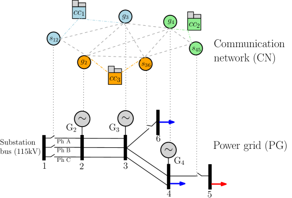
Let $G=(V,E)$ be an undirected graph that represents a distribution grid and its available upgrade options: $V$ and $E$ denote the set of buses and the set of distribution lines. The communication network, along with its potential upgrade options, is represented by a undirected graph $\widetilde{G}=(\widetilde{N},\widetilde{E})$, where $\widetilde{N}$ and $\widetilde{E}$ are the set of communication nodes and a set of communication links. A communication node is either a control point or an intermediate point. Each control point is associated with some device in $G$ and some nodes in $\widetilde{N}$ are designated as control centers.

The power grid $G$ depends on its communication network $\widetilde{G}$ in the following way: A device in $G$ (e.g., a generator or a RCSs) is operable only when its associated control point can receive a signal from some control center in $\widetilde{G}$. This modeling enables islands to form and to be operated independently only when at least one control center can communicate to the island and, in particular, its generator(s).

Let $\mathcal{G}=(\mathcal{N},\mathcal{E})$ be the integrated system of $G$ and $\widetilde{G}$ with $\mathcal{N}=N\cup\widetilde{N}$ and $\mathcal{E}=E\cup\widetilde{E}$. Let $\mathcal{D}$ be a set of damage scenarios for $\mathcal{G}$ indexed with $\mathcal{S}:=\{1,\cdots,|\mathcal{D}|\}.$ Each scenario $s\in\mathcal{S}$ is a set of edges of $\mathcal{E}$ that are damaged under $s$. The goal of the ORDPDC is to find an optimal upgrade profile for the cyber-physical system $\mathcal{G}$ that is resilient with respect to the damage scenarios in $\mathcal{D}$. The upgrade options include a) the building of new edges in $\mathcal{E}$ (i.e., distribution lines or communication links); b) the building of RCSs on some lines in $E$ to provide operational flexibility; c) the hardening of existing edges in $\mathcal{E}$ to lower the probability of damage, and d) the building of DGs at some buses of the grid.

The ORDPDC is a two-stage mixed integer stochastic program. The first-stage variables represent potential infrastructure enhancements for the coupled network $\mathcal{G}$ and the second-stage variables capture how upgrades serve the loads in each disaster scenario.

3.1 Mathematical Formulation

Table 3.1 specifies the input data for the ORDPDC problem, while Table 3.1 describes the model variables. The formulation assumes that all new lines come with switches (i.e., $\mathcal{E}_{x}^{n}\subseteq\mathcal{E}_{t}^{0}$) which reflects current industry practice. Throughout this paper, an edge $e\in\mathcal{E}$ is represented as an ordered pair $(e_{h},e_{t})$ for some $e_{h},e_{t}\in\mathcal{N}$ and $\delta(e)=\{e_{h},e_{t}\}$. The set of all edges incident to a node $i\in\mathcal{N}$ is denoted by $\delta(i)$. The notation $x_{\mathcal{A}}$ represents the projection of a vector $x$ to the space of some index set $\mathcal{A}$, i.e., $(x_{a})_{a\in\mathcal{A}}$: For instance, $x^{s}_{\mathcal{E}_{x}}=(x^{s}_{e})_{e\in\mathcal{E}_{x}}.$

The Parameters of the ORDPDC. $G=(N,E)$ an undirected extended distribution grid with available upgrade options $\mathcal{U}:=\mathcal{U}^{0}\cup\mathcal{U}^{n}$ a set of generators, indexed with $l$ $\qquad\mathcal{U}^{0}$ a set of existing generators $\qquad\mathcal{U}^{n}$ a set of generators that can be installed $i(l)\in N$ the bus in which the generator $l\in\mathcal{U}$ is located $\mathcal{U}_{i}\subseteq\mathcal{U}$ the set of generators connected to bus $i\in N$ $E_{V}\subseteq E$ a set of transformers $\beta_{e}$ maximum flow variation allowed between different phases on line $e\in E_{V}$ $\mathcal{C}\subseteq 2^{|E|}$ a collection of a set of edges which forms a cycle with a distinct node set $\mathcal{P}_{e},\mathcal{P}_{i},\mathcal{P}_{l}$ a set of phases on line $e\in E$, bus $i\in N$, and generator $l\in\mathcal{U}$, respectively $T_{e}^{k}$ a thermal limit on line $e\in E$ for phase $k\in\mathcal{P}_{e}$ $\underline{V}_{i}^{k},\overline{V}_{i}^{k}$ lower and upper bound on voltage magnitude at bus $i\in N$ on phase $k\in\mathcal{P}_{i}$ $Z_{e}=R_{e}+\mathbf{i}\ X_{e}$ phase impedance matrix of line $e\in E$ $\mathcal{L}\subseteq N$ a set of buses with critical loads $D_{i,p}^{k}+\mathbf{i}\ D_{i,q}^{k}$ complex power demand at bus $i\in N$ on phase $k\in\mathcal{P}_{i}$ $\eta_{c},\eta_{t}$ resiliency criteria in percentage for critical and total loads respectively $\overline{g}^{k}_{l,p}+\mathbf{i}\ \overline{g}^{k}_{l,q}$ complex power generation capacity of generator $l\in\mathcal{U}$ on phase $k\in\mathcal{P}_{l}$ $\widetilde{G}=(\widetilde{N},\widetilde{E})$ an extended associated communication network with potential upgrade options $\widetilde{N}_{c}:=\widetilde{N}_{t}\cup\widetilde{N}_{u}$ $\qquad\widetilde{N}_{t}\subseteq\widetilde{N}$ a set of control points for switches $\qquad\widetilde{N}_{u}\subseteq\widetilde{N}$ a set of control points for generators $\tilde{i}(e)\in\widetilde{N}_{t},\tilde{i}(l)\in\widetilde{N}_{u}$ the control point in $\widetilde{G}$ of a switch $e\in\mathcal{E}_{t}$ and a generator $l\in\mathcal{U}$, respectively $\tilde{i}_{d}\in\widetilde{N}$ an artificial dummy node in $\widetilde{G}$ $\mathcal{G}=(\mathcal{N},\mathcal{E})$ the integrated system of $G$ and $\widetilde{G}$ $\mathcal{E}_{x}:=\mathcal{E}_{x}^{0}\cup\mathcal{E}_{x}^{n}$ $\qquad\mathcal{E}_{x}^{0}\subseteq\mathcal{E}$ a set of existing lines and links $\qquad\mathcal{E}_{x}^{n}\subseteq\mathcal{E}$ a set of lines and links that can be installed $\mathcal{E}_{t}:=\mathcal{E}^{0}_{t}\cup\mathcal{E}^{n}_{t}$ $\qquad\mathcal{E}^{0}_{t}\subseteq E$ a set of lines in which a switch is installed $\qquad\mathcal{E}^{n}_{t}\subseteq E$ a set of lines in which a switch can be installed $\mathcal{E}_{h}\subseteq E$ a set of lines or links that can be hardened $c^{x}_{e}$ installation cost of $e\in\mathcal{E}_{x}^{n}$ $c^{t}_{e}$ installation cost of switch on $e\in\mathcal{E}^{n}_{t}$ $c^{h}_{e}$ line hardening cost of $e\in\mathcal{E}_{h}$ $c^{u}_{l}$ installation cost of $l\in\mathcal{U}^{n}$ on the corresponding bus $\mathcal{D}$ a collection of sets of damaged lines for each scenario, indexed with $\mathcal{S}:=\{1,\cdots,|\mathcal{D}|\}$

The Variables of the ORDPDC. Binary variables $x_{e}$ 1 if $e\in\mathcal{E}_{x}^{n}$ is built $t_{e}$ 1 if a switch is built on $e\in\mathcal{E}^{n}_{t}$ $h_{e}$ 1 if $e\in\mathcal{E}_{h}$ is hardened $u_{l}$ 1 if a generator $l\in\mathcal{U}^{n}$ is built. For each disaster scenario $s\in\mathcal{S}$, $z^{s}_{e}$ 1 if $e\in\mathcal{E}$ is active during $s$ $x^{s}_{e}$ 1 if $e\in\mathcal{E}_{x}$ exists during $s$ $t^{s}_{e}$ 1 if a switch on $e$ is used or not during $s$ $h^{s}_{e}$ 1 if $e\in\mathcal{E}_{h}$ is hardened during $s$ $u^{s}_{l}$ 1 if a generator $l\in\mathcal{U}^{n}$ is available during $s$ $y^{s}_{e}$ 1 if $i,\ j\in N$ can be disconnected, for $e=(i,j)\in C,\ C\in\mathcal{C}$, during $s$ $b_{e}$ 1 if the real power on line $e=(i,j)\in E$ flows from $j$ to $i$ during $s$ $b^{\prime}_{e}$ 1 if the reactive power on line $e=(i,j)\in E$ flows from $j$ to $i$ during $s$ Continuous variables For each disaster scenario $s\in\mathcal{S}$, $d^{s,k}_{i}=d^{s,k}_{i,p}+\mathbf{i}\ d^{s,k}_{i,q}$ amount of power delivered at bus $i\in N$ on phase $k\in\mathcal{P}_{i}$ during $s$ $g^{s,k}_{l}=g^{s,k}_{l,p}+\mathbf{i}\ g^{s,k}_{l,q}$ amount of power generation of $l\in\mathcal{U}$ on phase $k\in\mathcal{P}_{l}$ during $s$ $s^{s,k}_{e,i}=p^{s,k}_{e,i}+\mathbf{i}\ q^{s,k}_{e,i}$ power flow on $i$-end of line $e\in E$, where $i\in\delta(e)$, on phase $k\in\mathcal{P}_{e}$ during $s$ $V^{s,k}_{i}$ complex voltage at bus $i\in N$ on phase $k\in\mathcal{P}_{i}$ during $s$ $I^{s,k}_{e}$ complex current on line $e\in E$ on phase $k\in\mathcal{P}_{e}$ during $s$ $v_{i}^{s,k}$ squared voltage magnitude at bus $i\in N$ on phase $k\in\mathcal{P}_{i}$ during $s$ $f^{s}_{e}$ the amount of artificial flow on $e\in\widetilde{E}$ during $s$ $\gamma_{\tilde{i}}^{s}$ indicator of connectivity of control point $\tilde{i}\in\widetilde{N}$ to some control center during $s$

The presentation uses $w=(x_{\mathcal{E}^{n}_{x}},t_{\mathcal{E}^{n}_{t}},h_{\mathcal{E}_{h}},u_{\mathcal{U}^{n}})$ to denote upgrade profiles, $m$ the dimension of $w$, $c=(c^{x}_{\mathcal{E}^{n}_{x}},c^{t}_{\mathcal{E}^{n}_{t}},c^{h}_{\mathcal{E}_{h}},c^{u}_{\mathcal{U}^{n}})\in\mathbb{R}^{m}$ the cost vector, and $w^{s}=(x^{s}_{\mathcal{E}^{n}_{x}},t^{s}_{\mathcal{E}^{n}_{t}},h^{s}_{\mathcal{E}_{h}},u^{s}_{\mathcal{U}^{n}})$ feasible upgrade profiles for each scenario $s\in\mathcal{S}$. For each $s\in\mathcal{S},$ $\mathcal{Q}(s)$ denotes the set of upgrade profiles that enable the grid to maintain the predetermined load satisfaction (resiliency) level $\eta_{c},\eta_{t}$ (e.g., $\eta_{c}=0.98$ and $\eta_{t}=0.5$) under disaster scenario $s$.

With these notations, the ORDPDC is formulated as follows:

$$(P)\quad \min\quad c^{T}w$$ (1a)

s.t. $$w\geq w^{s}, \forall s\in\mathcal{S},$$ (1b)

$$w^{s}\in\mathcal{Q}(s),\ \forall s\in\mathcal{S},$$ (1c)

$$w\in\{0,1\}^{m}.$$

Problem ($P$) tries to find the optimal upgrade profile $w^{*}=(x^{*}_{\mathcal{E}^{n}_{x}},t^{*}_{\mathcal{E}^{n}_{t}},h^{*}_{\mathcal{E}_{h}},u^{*}_{\mathcal{U}^{n}})$ that ensures resilient operations for each disaster scenario. Equation (1b) ensures that an upgrade profile is feasible if it dominates a feasible solution $w^{s}\in\mathcal{Q}(s)$ for each scenario $s$, i.e., if the grid survives each of the extreme events in $\mathcal{S}$.

The set $\mathcal{Q}(s)$ is specified by resiliency constraints that are expressed in terms of the AC power flow equations, load satisfaction requirements, the communication network, and the grid topology:

$$\mathcal{Q}(s)=\{w^{s}\in\{0,1\}^{m}:(2),(3),\eqref{eq:generator/demand},(5),\mbox{ and }\eqref{eq:topology}\}$$

where Constraints (2), (3), (4), (5), and (6) are stated in detail in the following. The variables in each $\mathcal{Q}(s)$ are indexed by $s$. For simplicity, this section omits index $s$.

3.1.1 Power Flow Constraints

Figure 2: Notations for the Power Flow Equations.

Figure 2 specifies the power flow equations and summarizes some of the notations. Let $\mathcal{P}=\{a,b,c\}$ denote the three phases of the network. For each bus $i\in N$, define $V_{i}=(V_{i}^{k})_{k\in\mathcal{P}_{i}}$ and, for each line $e\in E$, define $I_{e}=(I_{e}^{k})_{k\in\mathcal{P}_{e}}$ and $s_{e,i}=(s_{e,i}^{k})_{k\in\mathcal{P}_{e}}$. The notations also use a superscript $\mathcal{P}^{\prime}\subseteq\mathcal{P}$ to represent the projection or the extension of a vector to the space of $\mathcal{P}^{\prime}$. For example, if $\mathcal{P}_{i}=\{a,b,c\}$ and $\mathcal{P}^{\prime}=\{a,b\}$, then $V_{i}^{\mathcal{P}^{\prime}}=\left(V_{i}^{a},V_{i}^{b}\right)^{T}$. If $\mathcal{P}_{i}=\{a,c\}$ and $\mathcal{P}^{\prime}=\{a,b,c\}$, then $V_{i}^{\mathcal{P}^{\prime}}=\left(V_{i}^{a},0,V_{i}^{c}\right)^{T}.$

For each line $e=(i,j)\in E$, Ohm’s law for 3-phase lines states the relationship $V_{j}^{\mathcal{P}_{e}}=V_{i}^{\mathcal{P}_{e}}-Z_{e}I_{e}$ between $I_{e}$, $V_{i}$, and $V_{j}$. For each line $e\in E$ and bus $i\in\delta(e)$, the electric power flow equation $s_{e,i}=\mbox{diag}(V_{i}^{\mathcal{P}_{e}}I_{e}^{H})$ describes the relationship between $s_{e,i}$, $V_{i}^{\mathcal{P}_{e}}$, and $I_{e}$, where superscript $H$ indicates the conjugate transpose. In Figure 2, the big-M method is used in Equations (2a) to apply Ohm’s law only for available lines; the big-M can be set as $\max_{j^{\prime}\in\{i,j\},k\in\mathcal{P}_{e}}\overline{V}_{j^{\prime}}^{k}-\min_{j^{\prime}\in\{i,j\},k\in\mathcal{P}_{e}}\underline{V}^{k}_{j^{\prime}}$. Equations (2c) is the balance equation for power flow at each bus $i\in N$, i.e., the sum of incoming flows equals the sum of the outgoing flows.

Let $p_{e,i}+\textbf{i}q_{e,i}$ be the rectangular representation of $s_{e,i}$, where $p_{e,i}=(p_{e,i}^{k})_{k\in\mathcal{P}_{i}}$ and $q_{e,i}=(q_{e,i}^{k})_{k\in\mathcal{P}_{i}}$ denote the real and reactive power at the $i$-end of line $e$. Equations (2d) and (2e) specify the thermal limits on lines and the voltage bounds on buses.

In some disaster scenarios when some of the lines are broken, power flows of different phases on the same line can have opposite directions, which is a very undesirable operationally. Equations (2f) and (2g) prevent this behavior from happening.

The real and reactive power on different phase must stay within a certain limit. Let $\widehat{p}_{e,i}=\sum_{\tilde{k}\in\mathcal{P}_{e}}p_{e,i}^{\tilde{k}}$ and $\widehat{q}_{e,i}=\sum_{\tilde{k}\in\mathcal{P}_{e}}q_{e,i}^{\tilde{k}}$. Then, these limits are formulated as follows:

$$\left(\underline{\beta}_{e}(1-b_{e})+\overline{\beta}_{e}b_{e}\right)\frac{\widehat{p}_{e,i}}{|\mathcal{P}_{e}|}\leq{p}_{e,i}^{k}\leq\left(\underline{\beta}_{e}b_{e}+\overline{\beta}_{e}(1-b_{e})\right)\frac{\widehat{p}_{e,i}}{|\mathcal{P}_{e}|}, \ \forall e\in E_{V},k\in\mathcal{P}_{e},$$ (3a)

$$\left(\underline{\beta}_{e}(1-b^{\prime}_{e})+\overline{\beta}_{e}b^{\prime}_{e}\right)\frac{\widehat{q}_{e,i}}{|\mathcal{P}_{e}|}\leq{q}_{e,i}^{k}\leq\left(\underline{\beta}_{e}b^{\prime}_{e}+\overline{\beta}_{e}(1-b^{\prime}_{e})\right)\frac{\widehat{q}_{e,i}}{|\mathcal{P}_{e}|}, \ \forall e\in E_{V},k\in\mathcal{P}_{e},$$ (3b)

where $\underline{\beta}_{e}=1-\beta_{e}$ and $\overline{\beta}_{e}=1+\beta_{2}$.

3.1.2 Generator/resiliency Constraints

Moreover, each generator $l\in\mathcal{U}$ has its own capacity and at least some percentage of critical and total loads must be satisfied as specified by the resiliency criteria $\eta_{c}$ and $\eta_{t}$.

$$0\leq g_{l,p}^{k}\leq\overline{g}^{k}_{l,p}u_{l},\ g_{l,q}^{k}\leq\overline{g}^{k}_{l,q}u_{l}, \forall l\in\mathcal{U},k\in\mathcal{P}_{l},$$ (4a)

$$0\leq d_{i,p}^{k}\leq D_{i,p}^{k},\ 0\leq d_{i,q}^{k}\leq D_{i,q}^{k}, ~{}\forall i\in N,k\in\mathcal{P}_{i}$$ (4b)

$$\sum_{i\in\mathcal{L}}d^{k}_{i,p}\geq\eta_{c}\sum_{i\in\mathcal{L}}D^{k}_{i,p},\quad\sum_{i\in\mathcal{L}}d^{k}_{i,q}\geq\eta_{c}\sum_{i\in\mathcal{L}}D^{k}_{i,q}, \quad\forall k\in\mathcal{P},$$ (4c)

$$\sum_{i\in N}d^{k}_{i,p}\geq\eta_{t}\sum_{i\in N}D^{k}_{i,p},\quad\sum_{i\in N}d^{k}_{i,q}\geq\eta_{t}\sum_{i\in N}D^{k}_{i,q}, \forall k\in\mathcal{P}.$$ (4d)

Equation (4a) captures the power generation capacity constraints. Equation (4b) states that the delivered power at each bus $i$ should not exceed the load. Equations (4c)-(4d) enforce the resiliency constraints.

3.1.3 Communication Constraints

Figure 3: The Single-Commodity Flow Model for $\widetilde{G}$ (red-colored squares denote control centers).

The operation of generators and RCSs depend on the communication network: A generator $l\in\mathcal{U}$ and a RCS on line $e\in\mathcal{E}_{t}$ is operable only if their associated control points $\tilde{i}(l)\in\widetilde{N}$ and $\tilde{i}(e)\in\widetilde{N}$ can receive a control signal from some control centers through $\widetilde{G}$. To capture the connectivity of a vertex to some control centers, the formulation uses a single-commodity flow model summarized in Equations (5) in Figure 3. The formulation uses a dummy node $\tilde{i}_{d}$ to $\widetilde{N}$ and connect $\tilde{i}_{d}$ to all control centers with additional links. The flow $f\in\mathbb{R}^{|\widetilde{E}|}$ originating from the dummy node $\tilde{i}_{d}$ then is used to check the connectivity of every node. By Equation (5c), the flow passes only through available links during disaster $s$ (the big-M value is set to $|\widetilde{N}_{c}|$ in the implementation). If a control point $i\in\widetilde{N}_{c}$ is connected with some control center through some path, it can borrow a unit of flow from $f$ to make $\gamma_{i}$ 1, as specified in Equations (5a) and (5b). In other words, $\gamma_{i}$ indicates whether control point $i\in\widetilde{N}_{c}$ can receive a control signal. If $\gamma_{i}$ is 1, the associated device in $G$ is operable by Equations (5d) and (5e).

Some communication network may be affected by a failure in distribution grid, e.g., when the grid fails to supply power to communication centers. This kind of dependencies is not considered in this paper but it can be easily captured if needed. Indeed, first assign a small critical load to each communication center and add constraints that restrict the auxiliary arcs between the dummy node and each communication center to have positive flow only when the associated communication center has a positive power supply. The constraints can be expressed in terms of an extra binary variable for each bus at which a communication center is located. The extra binary variable determines if there is a positive power supply to the communication center.

3.1.4 Topological constraints.

The final set of constraints captures the topology restrictions in distribution systems:

$$x_{e}\geq t_{e}, \forall e\in\mathcal{E},$$ (6a)

$$z_{e}=x_{e}-t_{e},\hskip 113.81102pt \forall e\in\mathcal{E},$$ (6b)

$$x_{e}=h_{e}, \forall e\in\mathcal{D}_{s},$$ (6c)

$$\sum_{e\in C}y_{e}\leq|C|-1, \forall C\in\mathcal{C},$$ (6d)

$$z_{\hat{e}}\leq y_{e}, \forall\hat{e}\in E:\delta(\hat{e})=\delta(e),\ e\in C,\ C\in\mathcal{C}.$$ (6e)

Constraint (6a) restrict switches to be operable only on existing lines. In Equation (6b), $z_{e}$ represents whether line $e\in\mathcal{E}$ is active under scenario $s$. A line is active when it exists and its switch is off. Equation (6c) states that a damaged line during scenario $s\in\mathcal{S}$ is inoperable unless it is hardened. Constraints (6d) and (6e) ensures that the distribution grid should operate in a radial manner. Accordingly, Constraint (6d) eliminates the sub-tours within $\mathcal{C}$. Since $G$ is usually sparse, the implementation enumerates all the sub-tours $\mathcal{C}$ and variable $y_{e}$ indicates whether $i,j\in\delta(e)$ are disconnected. If they are disconnected, then all the lines between $i$ and $j$ are inactive by Constraint (6e).

Note also that, for existing lines not damaged under scenario $s$, $x_{e}$ is fixed as one. For each line $e\in E\setminus\mathcal{E}_{t}$, $t_{e}$ is set to zero. Finally, for each line $e\in\mathcal{E}\setminus\mathcal{E}_{h},$ $h_{e}$ is fixed as 0 and all the existing generators have $u_{l}=1$. This paper assumes perfect hardening, i.e., a hardened line survives all disaster scenarios. This assumption can be naturally generalized to imperfect hardening (Yamangil et al. 2015).

4 Linearization of the ORDPDC

The formulation of the ORDPDC is nonlinear. This section discusses how to obtain an accurate linearization.

4.1 Linear Approximation of the AC Power Flow Equations for Radial Networks

The main difficulty lies in linearizing constraints (2a–2b) for which the formulation uses the tight linearization from Gan and Low (2014). The linearization is based on two assumptions: (A1) line losses are small, i.e., $Z_{e}I_{e}I_{e}^{H}\approx 0$ for $e=(i,j)\in E$ and (A2) voltages are nearly balanced, i.e., if $\mathcal{P}_{i}=\{a,b,c\}$, then $V^{a}_{i}/V^{b}_{i}\approx V^{b}_{i}/V^{c}_{i}\approx V^{c}_{i}/V^{a}_{i}\approx e^{i2\pi/3}.$ Informally speaking, the approximation generalizes the distflow equations to 3 phases, drops the quadratic terms, and eliminates the current variables using the balance assumption. The derivation assumes that all phases are well-defined for simplicity. Moreover, if $A$ is an $n\times n$ matrix, then diag($A$) denotes the $n$-dimensional vector that represents its diagonal entries. If $a$ is an $n$-dimensional vector, then diag($a$) denotes the $n\times n$ matrix with $a$ in its diagonal entries and zero for the off-diagonal entries.

Let $s_{i}=\sum_{l\in\mathcal{U}_{i}}g_{l}-d_{i}$ denote the power injection at bus $i$. By (A1), $s_{e,i}=s_{e,j}$ for all $e\in(i,j)\in E$ and therefore, given $s_{i}$, $s_{e,i}$ ($i\in\delta(e))$ is uniquely determined by Equation (2c).

Now define $S_{e,i}:=V_{i}I_{e}^{H}$, whose diagonal entries are $s_{e,i}$. Multipling both sides of $V_{j}=V_{i}-Z_{e}I_{e}$ with their conjugate transposes gives

$$V_{j}V_{j}^{H}=V_{i}V_{i}^{H}-S_{e,i}Z_{e}^{H}-Z_{e}S_{e,i}^{H}+Z_{e}I_{e}I_{e}^{H}Z_{e}^{H}.$$ (7)

By assumption (A1), this becomes

$$V_{j}V_{j}^{H}=V_{i}V_{i}^{H}-S_{e,i}Z_{e}^{H}-Z_{e}S_{e,i}^{H}$$ (8)

and, by restricting attention to diagonal elements only,

$$v_{j}=v_{i}-\mbox{diag}(S_{e,i}Z_{e}^{H}-Z_{e}S_{e,i}^{H}).$$ (9)

where $(v^{k}_{i})_{k\in\mathcal{P}_{i}}=\mbox{diag}(V_{i}V_{i}^{H})$ represents the squared voltage magnitude at bus $i\in N$.

By (A2), we have $S_{e,i}\approx\gamma^{\mathcal{P}_{e}}\mbox{diag}(s_{e,i}),$ where

$$\gamma=\left[\begin{array}[]{ccc}1&\alpha^{2}&\alpha\\ \alpha&1&\alpha^{2}\\ \alpha^{2}&\alpha&1\end{array}\right]\mbox{ and }\alpha=e^{-i2\pi/3}.$$

As a result, Equation (9) can now be simplified as follows: for each line $e=(i,j)\in E$ and $k\in\mathcal{P}_{e}$,

$$v^{k}_{i}=v^{k}_{j}-\sum_{k^{\prime}\in\mathcal{P}_{e}}2\left[(\alpha^{n_{k}-n_{k^{\prime}}}R_{e})^{kk^{\prime}}p_{e,i}^{k^{\prime}}+(\alpha^{n_{k}-n_{k^{\prime}}}X_{e})^{kk^{\prime}}q_{e,i}^{k^{\prime}}\right],$$ (10)

where $n_{a}=2,n_{b}=1,n_{c}=0$, $R_{e}+\textbf{i}X_{e}=Z_{e}$, and superscript $kk^{\prime}$ of a matrix denotes its $(k,k^{\prime})$-entry.

In summary, Ohm’s law and the power flow equation in Constraints (2a) and (2b) are approximated by Eq. (10) for all $e=(i,j)\in E$ and $k\in\mathcal{P}_{e}$ and the big-$M$ is set to $\max_{j^{\prime}=i,j}(\overline{V}_{j^{\prime},k})^{2}-\min_{j^{\prime}=i,j}(\underline{V}_{j^{\prime},k})^{2}$, along with Equation (2c). Accordingly, Constraint (2e) is replaced by the following constraint:

$$(\underline{V}_{i}^{k})^{2}\leq v_{i}^{k}\leq(\overline{V}_{i}^{k})^{2},\quad\forall i\in N,k\in\mathcal{P}_{i}.$$

4.2 Linearization of (3a)-(3b)

Constraints (3a) and (3b) contain products of a binary variable and a bounded real variable. These constraints are linearized without loss of accuracy using McCormick inequalities McCormick (1976).

4.3 Piecewise-Linear Inner Approximation of Thermal Limits

Figure 4: The Piecewise-Linear Inner Approximation of a Circle.

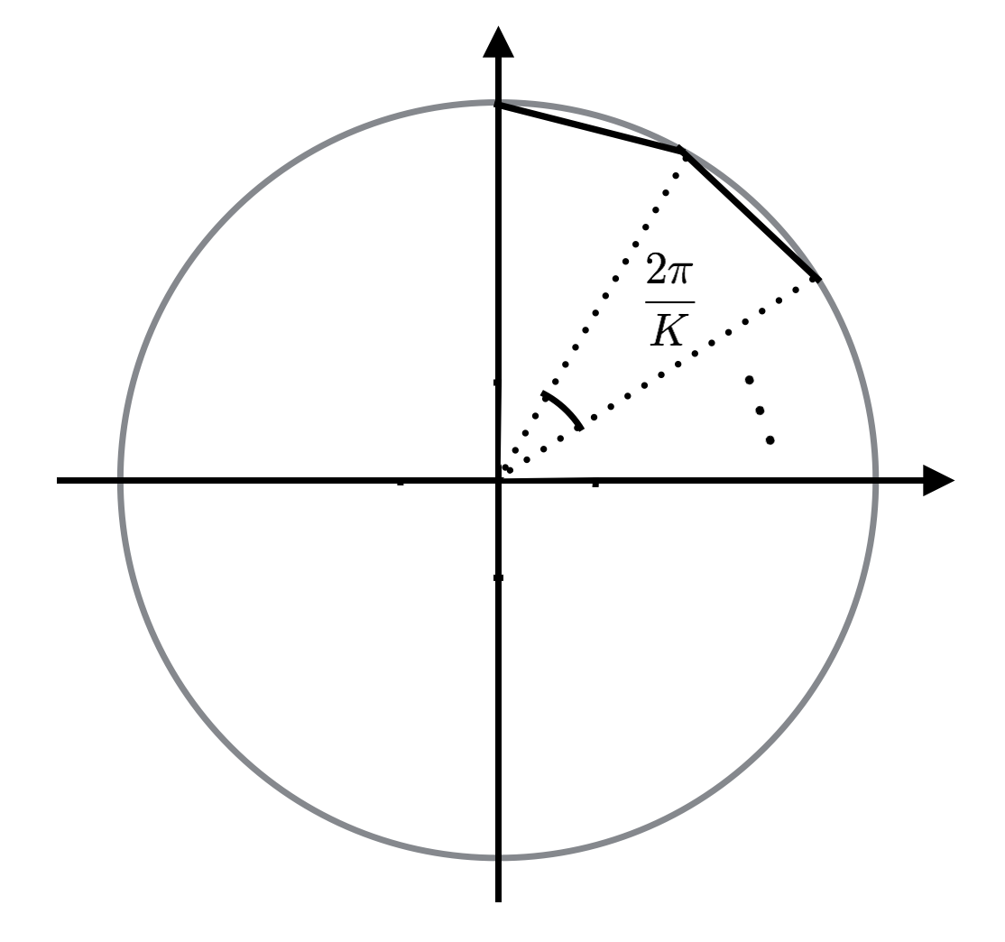
The quadratic thermal limit constraints (Constraint (2d)) can be approximated with $K$ linear inequalities as shown in Figure 4. The resulting inequalities are as follows: for all $e\in E$, $i\in\delta(e)$, $k\in\mathcal{P}_{e}$:

$$\left(\sin\left(\frac{2n\pi}{K}\right)-\sin\left(\frac{2(n-1)\pi}{K}\right)\right)p_{e,i}^{k}$$

$$-\left(\cos\left(\frac{2n\pi}{K}\right)-\cos\left(\frac{2(n-1)\pi}{K}\right)\right)q_{e,i}^{k}\leq\sin\left(\frac{2\pi}{K}\right)T_{e,k}, \ \forall n=1,\cdots,K,$$ (11a)

$$-Mz^{s}_{e}\leq p_{e,i}^{k}\leq Mz^{s}_{e},\quad-Mz^{s}_{e}\leq q_{e,i}^{k}\leq Mz^{s}_{e}, \quad\forall e\in E,k\in\mathcal{P}_{e}.$$ (11b)

where the big-M is set to $\sum_{i\in N}D^{p}_{i,k}$. Our implementation uses $K=28$.

5 Scenario-Based Decomposition

In Section 9, the branch and price algorithm presented in the next section is compared to the Scenario-Based Decomposition (SBD) algorithm proposed by Nagarajan et al. (2016). SBD iteratively solves a master problem $P(\mathcal{S}^{\prime})$ which only includes the constraints of a subset of scenarios $\mathcal{S}^{\prime}\subseteq\mathcal{S}$. The algorithm terminates when the optimal solution to $P(\mathcal{S}^{\prime})$ is feasible (and hence optimal) for the remaining scenarios $\mathcal{S}\setminus\mathcal{S}^{\prime}$. Otherwise, at least one scenario $s\in\mathcal{S}\setminus\mathcal{S}^{\prime}$ is infeasible. Scenario $s$ is added to $\mathcal{S}^{\prime}$ and the process is repeated.

6 The Branch-and-Price Algorithm

This paper proposes a branch-and-price (B&P) algorithm for the ORDPDC. The B&P exploits the special structure of the ORDPDC in several ways. First, it uses a compact reformulation that yields a better lower bound than the LP relaxation. The reformulation also makes it possible to use column generation and solve independent pricing problems associated with each scenario in parallel. Finally, several additional techniques are used to accelarate the column generation significantly. Section 6.1 presents the problem reformulation and Section 6.2 briefly reviews the basic column generation of the B&P algorithm. Section 6.3 introduces several acceleration schemes. The implementation of the B&P algorithm is presented in Section 6.4.

6.1 The Problem Reformulation

Letting $\widetilde{\mathcal{Q}}(s)$ be the linearization of $\mathcal{Q}(s)$, the problem ($P$) is rewritten as

$$(P)\quad c^{T}w$$ min

s.t. $$w-w^{s}\geq 0, \ \forall s\in\mathcal{S},$$ (12a)

$$w^{s}\in\widetilde{\mathcal{Q}}(s), \ \forall s\in\mathcal{S},$$ (12b)

$$w^{s}\in\{0,1\}^{m}, \ \forall s\in\mathcal{S}.$$ (12c)

Without the linking constraint (12a), ($P$) can be decomposed into $|\mathcal{S}|$ independent problems, each of which has a feasible region defined by

$$\mathcal{P}^{s}=\left\{w^{s}\in\mathbb{R}^{m}:\eqref{eq:sub}\mbox{ and }\eqref{eq:binary}\right\},\ \forall s\in\mathcal{S}.$$

Observe that $\mathcal{P}^{s}$ is bounded and let $\mathcal{J}^{s}=\{\hat{w}^{s}_{j}\in\mathbb{R}^{m}:\hat{w}^{s}_{j}\mbox{ is a vertex of }\mbox{conv}(\mathcal{P}^{s})\}$ be the set of all vertices of conv($\mathcal{P}^{s}$). Letting $\mathcal{J}=\cup_{s}\mathcal{J}_{s}$, consider the following problem:

$$(\widetilde{P})\quad c^{T}w$$ min

s.t. $$w \quad-\sum_{j\in\mathcal{J}^{s}}\lambda_{j}^{s}\hat{w}_{j}^{s}\geq 0,\ \forall s\in\mathcal{S},$$ (13a)

$$\quad\sum_{j\in\mathcal{J}^{s}}\lambda_{j}^{s}=1, \forall s\in\mathcal{S},$$ (13b)

$$\quad w\in\{0,1\}^{m},$$ (13c)

$$\quad\lambda^{s}_{j}\geq 0, \forall j\in\mathcal{J}^{s},s\in\mathcal{S}.$$ (13d)

Theorem 6.1

($P$) and ($\widetilde{P}$) are equivalent.

Proof. Since ($P$) and ($\widetilde{P}$) have the same objective function, it suffices to show that ($P$) has an optimal solution that is feasible to ($\widetilde{P}$) and vice versa. Let $(\bar{w},\{\bar{w}^{s}\}_{s\in\mathcal{S}})$ be the optimal solution of ($P$). By the Farkas-Minkowski-Weyl theorem (Schrijver 1998), $\bar{w}^{s}$ can be expressed as a convex combination of some extreme points in $\mathcal{J}^{s}$, for each $s\in\mathcal{S}$. Hence, we can construct a feasible solution of ($\widetilde{P}$) from $(\bar{w},\{\bar{w}^{s}\}_{s\in\mathcal{S}})$.

Consider now an optimal solution of ($\widetilde{P}$), $(\bar{w}^{\prime},\{\bar{\lambda}^{s\prime}_{j}\}_{j\in\mathcal{J}^{s}}\mbox{ for }s\in\mathcal{S})$. By (13a), if $\bar{\lambda}^{s\prime}_{j}>0$ for $j\in\mathcal{J}^{s}$, $\hat{w}^{s}_{j}$ is dominated by $\bar{w}^{\prime}.$ Therefore, it is possible to construct another optimal solution to ($\widetilde{P}$) by choosing a single $j^{*}$ for which $\bar{\lambda}^{s\prime}_{j^{*}}>0$ for each $s\in\mathcal{S}$, setting $\bar{\lambda}^{s\prime}_{j^{*}}$ to one and setting the other $\bar{\lambda}^{s\prime}_{j}$ to zero. By definition of $\mathcal{J}_{s}$, the constructed optimal solution is feasible for ($P$). $\square$

This paper uses a branch-and-price algorithm to solve ($\widetilde{P}$). Let $LP_{\widetilde{P}}$ denote the LP relaxation of ($\widetilde{P}$). Since the feasible region of ($\widetilde{P}$) is the intersection of the convex hulls of each subproblem, $LP_{\widetilde{P}}$ yields a stronger lower bound than the LP relaxation of ($P$).

6.2 The Basic Branch and Price

The B&P algorithm uses a restricted master problem ($M$) with a subset of columns of ($\widetilde{P}$) and $|\mathcal{S}|$ independent subproblems ($P_{s}$) for $s\in\mathcal{S}$, instead of handling $LP_{\widetilde{P}}$ globally. The column generation starts with an initial basis that consists of the first-stage variables $w$, a column associated with a feasible solution for each subproblem, and some slack variables. Let $\widetilde{\mathcal{J}}^{s}$ be the corresponding subset of $\mathcal{J}^{s}$. The restricted mater problem ($M$) is as follows:

$$(M)\quad c^{T}w$$ min

s.t. $$w- \sum_{j\in\widetilde{\mathcal{J}}^{s}}\lambda_{j}^{s}\hat{w}_{j}^{s}\geq 0, \ \forall s\in\mathcal{S},$$ (14a)

$$\sum_{j\in\widetilde{\mathcal{J}}^{s}}\lambda_{j}^{s}=1, \forall s\in\mathcal{S},$$ (14b)

$$w\geq 0,\$$ (14c)

$$\lambda^{s}_{j}\geq 0,\quad \forall j\in\widetilde{\mathcal{J}}^{s},\ \forall s\in\mathcal{S}.$$ (14d)

and the pricing problem for scenario $s$ is specified as follows:

$$\begin{array}[]{lll}(P_{s})&\ \min&\ -\bar{\sigma}^{s}\ +{\bar{y}^{sT}}\ w^{s}\\ &\mbox{s.t.}&\ w^{s}\in\widetilde{\mathcal{Q}}(s),\\ &&\ w^{s}\in\{0,1\}^{m},\end{array}$$

where, for a scenario $s$, $\bar{y}^{s}$ is the dual solution for constraints (14a) and $\bar{\sigma}^{s}$ is the dual solution of the convexity constraint (14b).

6.3 Acceleration Schemes

The performance of column generation deteriorates when the master problem exhibits degeneracy, leading to multiple dual solutions which may significantly influence the quality of columns generated by the pricing problem. The master problem $(M)$ suffers from degeneracy, especially early in the column-generation process. Initially, ($M$) has $(m+1)|\mathcal{S}|$ constraints, $m$ columns corresponding to the first-stage variables $w$, and $|\mathcal{S}|$ columns for the second-stage variables $\{\lambda^{s}\}_{s\in\mathcal{S}}$. Therefore, in early iterations, linear solvers have a natural tendency to select $m(|\mathcal{S}|-1)$ columns from the slack variables in Constraints (14a). For example, assume that the slack variable is in basis for the constraint involving a non-basic first-stage variable $w_{k}$ and a scenario $s$ in Constraints (14a). By complementary slackness, this implies that the dual variable is zero. Consider a vertex $\hat{w}^{s}$ whose $k$-th entry is non-zero. The value $\bar{y}^{s}_{k}w^{s}_{k}$ is zero in the pricing problem. However, for this vertex to enter the basis, it must incur the cost $c_{k}$ of $w_{k}$, which is ignored in the pricing subproblem. As a result, subproblem ($P_{s}$) prices many columns too optimistically and generates columns that do not improve the current objective value, resulting in a large number of iterations.

6.3.1 Pessimistic Reduced Cost

In order to overcome the poor pricing of columns, this section first proposes a pessimistic pricing scheme that selects more meaningful columns in early iterations. Consider a solution $w^{s}$ to the pricing problem. If $w^{s}_{k}=1$ but the first-stage variable $w_{k}$ is not in basis, then by the relevant constraint from $\eqref{eq:m_link}$, the variable $\lambda_{j}^{s}$ corresponding to $w^{s}$ can only enter in the basis at 1 if $w_{k}$ is also in the basis at 1. As a result, the pessimistic pricing scheme adds the reduced cost $c_{k}-\sum_{s\in\mathcal{S}}\bar{y}^{s}_{k}$ to the pricing objective, which becomes

$$-\bar{\sigma}^{s}+(\bar{y}^{s})^{T}w^{s}+\sum_{k\in\eta}(c_{k}-\sum_{s\in\mathcal{S}}\bar{y}^{s}_{k})w^{s}_{k}$$

where $\eta$ is the set of non-basic first-stage variables, i.e., $\eta=\{k\ |\ w_{k}\mbox{ is non-basic}\}.$ Note that column generation with this pessimistic pricing subproblem is not guaranteed to converge to the optimal linear relaxation. Hence, the implementation switches to the standard pricing problem in later iterations.

6.3.2 Optimality Cut

A solution to the master problem ($M$) where the first-stage variables take integer value gives an upper bound to the optimal solution. The B&P algorithm periodically solves the integer version of ($M$) to obtain its objective value $\bar{v}(M)$. The constraint

$$c^{T}w^{s}\leq\bar{v}(M)$$

can then be added to the pricing subproblem for scenario $s$ since any solution violating this constraint is necessarily suboptimal. As shown later on, this optimal cut is critical to link the two phases of the column generation, preventing many potential columns to be generated in the second phase.

6.3.3 A Lexicographic Objective for Pricing Subproblems

In general, sparse columns are more likely to enter the basis in the master problem ($M$). As a result, the B&P algorithm uses a lexicographic objective in the pricing subproblem. First, it minimizes the (pessimistic or standard) reduced cost. Then it maximizes sparsity by minimizing $1^{T}w^{s}$ subject to the constraint that the reduced cost must be equal to the optimal objective value of the first stage.

6.4 The Final Branch and Price Implementation

6.4.1 Column Generation

The column generation starts with an initial basis built from the optimal solutions of each subproblems under the objective function of $c^{T}w^{s}$. It then proceeds with two phases of column generation, first using the pessimistic reduced cost and then switching to the standard one.

The second phase terminates when the optimality gap becomes lower than the predetermined tolerance, e.g., $0.1\%$. The lower bound is based on Lagrangian relaxation. Given a pair $\bar{w}$ and $(\bar{y},\bar{\sigma})$ of optimal primal and dual solutions for ($M$), the Lagrangian relaxation is given by

$$L(\bar{w},\bar{y},\bar{\sigma})=c^{T}\bar{w}+\sum_{s\in\mathcal{S}}{\cal O}_{s}(\bar{y},\bar{\sigma})$$

where ${\cal O}_{s}(\bar{y},\bar{\sigma})$ is the optimal solution of the pricing problem for scenario $s$ under dual variables $(\bar{y},\bar{\sigma})$. The first phase uses the same technique for termination, although the resulting formula is no longer guaranteed to be a lower bound. Once the gap between the upper bound and the “approximate” lower bound is smaller than the tolerance, the column generation process moves to the second phase.

The column generation also avoids generating dominated columns. Assume that $[w^{s}_{1}=1,w^{s}_{2}=1]$ is a feasible solution of $(P_{s})$ and the corresponding column has been added to the master problem ($M$). Then, there is no need to consider a solution $[w^{s}_{1}=1,w^{s}_{2}=1,w^{s}_{3}=1]$. The column generation adds the constraint of $w^{s}_{1}+w^{s}_{2}\leq 1$ to $(P_{s})$ when such a dominated solution is produced and does not include it in the master problem.

6.4.2 The Branch and Bound

After convergence of the column generation to $LP_{\widetilde{P}}$, the branch and bound algorithm solves the restricted master problem ($M$) with the integral condition $w\in\{0,1\}^{m}$ to obtain a strong primal bound. In general, this incumbent solution is of very high quality and the average optimality gap is 0.19%. Therefore, the branch and price algorithm uses a depth-first branch and bound. Moreover, at each branching node, it selects the variable that minimizes the optimality gap.

7 Description of the Data Sets

This section describes the distribution test systems. The data set is available from https://github.com/lanl-ansi/micot/ in the application_data/lpnorm directory. Details of the data format are available from https://github.com/lanl-ansi/micot/wiki/Resilient-Design-Executable.

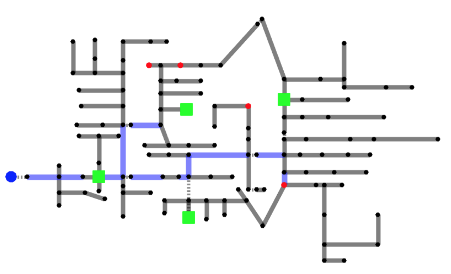
The first two sets, the Rural and Urban systems, is from Yamangil et al. (2015). They are based on the IEEE 34 bus system (Kersting 1991) (see Figure 5) and replicate the 34-bus distribution feeder three times. All three feeders are connected to a single transmission bus and candidate new lines were added to the network to allow back-feeds. In the rural model, the distribution feeder was geolocated to model feeders with long distances between nodes. Similarly, the urban network was geolocated to model compact feeders typical of urban environments. Geolocation of these networks has the net effect of adjusting the lengths of the power lines and their associated impedance values. Spreading the network out also increases the hardening and new line costs. As a result, the rural system is expected to favor solutions with distributed generation and the urban system solutions with new lines and switches (in addition to hardening lines). The fixed cost of installing a new distributed generator is set at $500k. The cost of a distributed generator is set at $1,500k per MW based on the 2025 projections from U.S. Energy Information Administration (2014). The cost of installing new switches for 3-phase lines is set between 10k and 50k (Bialek 2014). The cost of new underground 3-phase lines is set at about $500k per mile and the cost of new underground single phase lines is set at about $100k per mile. The hardening cost was set at roughly $50k and $10k per mile for multi-phase and single-phase lines (State of Virginia Corporation Commission 2005). The third network, network123, is based on the 123-node network of Kersting (1991). This network was unaltered except for adding new line candidates and labeling large loads as critical.

(a) Urban

(b) Rural

Figure 5: The urban and rural distribution systems which contain three copies of the IEEE 34 system to mimic situations where there are three normally independent distribution circuits that support each other during extreme events. These test cases include 109 nodes, 118 generators, 204 loads, and 148 edges.

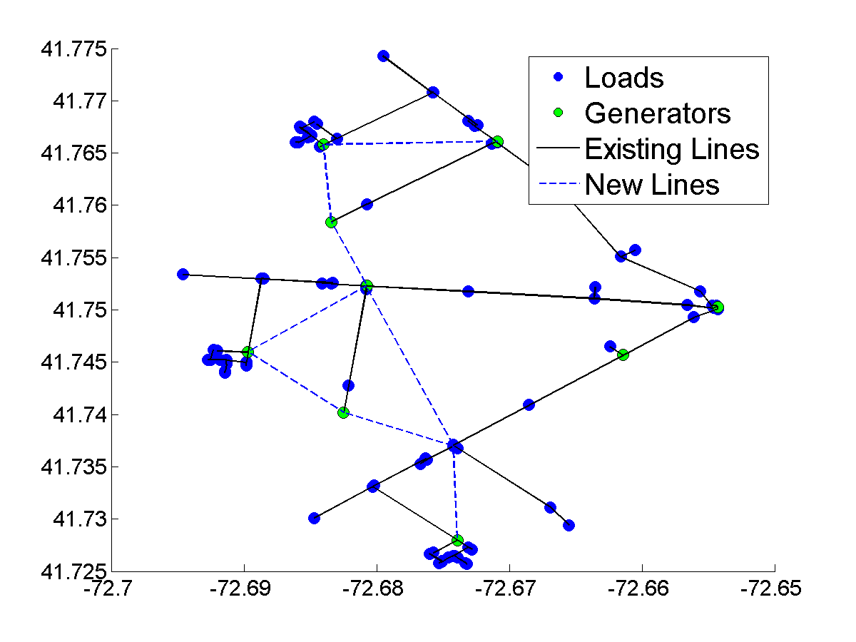
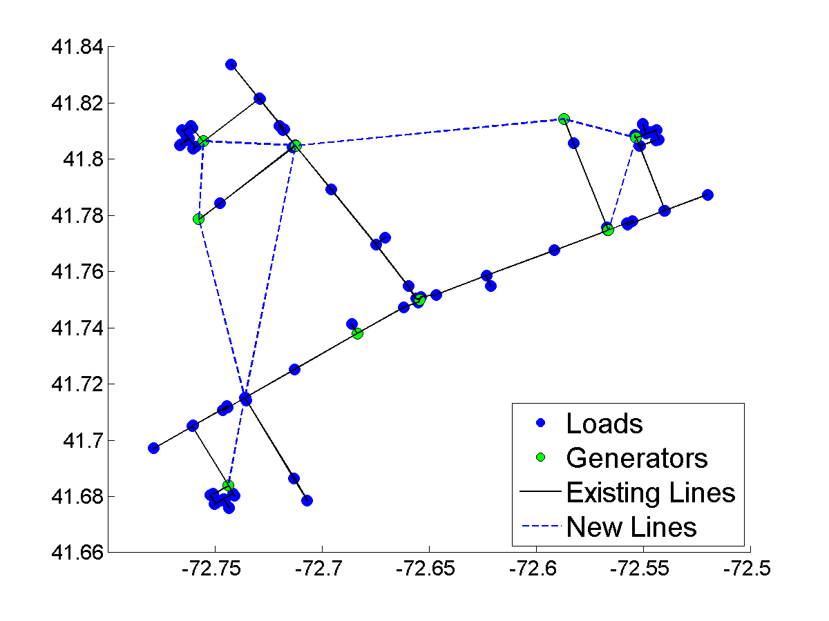
The communication network $\widetilde{G}$ is built to conform to $G$. Let $G^{\prime}=(N^{\prime},E^{\prime})$ be the duplicate of $G$. For each generator $l\in\mathcal{U}$, its duplicate $i(l)$ represents its control point. Consider $\mathcal{E}^{\prime}_{t}\subseteq E^{\prime}$, the duplicate of $\mathcal{E}_{t}$. To represent the control point for a switch, $e\in\mathcal{E}^{\prime}_{t}$ is divided in the middle and a new vertex $v_{e}$ is added to represent the control point for the switch. In other words, the edge $e=(e_{h},e_{t})\in\mathcal{E}^{\prime}_{t}$ is replaced by a new vertex $v_{e}$ and two new edges $e_{1}=(e_{h},v_{e}),e_{2}=(v_{e},e_{t})$. The test cases assume that the damage, installation, and hardening of a line in $G$ are also incurred for the corresponding line in $\widetilde{G}$. These assumptions can be easily generalized without changing the nature of the model.

The experimental evaluation considers 100 scenarios per damage intensity for all three networks and the damage intensities are taken in the set $\{1\%,$ $2\%,$ $3\%,$ $4\%,$ $5\%,$ $10\%,$ $15\%,$ $20\%,$ $25\%,$ $30\%,$ $35\%,$ $40\%,$ $45\%,$ $50\%,$ $55\%,$ $60\%,$ $65\%,$ $70\%,$ $75\%,$ $80\%,$ $85\%,$ $90\%,$ $95\%,$ $100\%\}$. The scenario generation procedure is based on damage caused by ice storms. The intensity tends to be homogeneous on the scale of distribution systems (Sa 2002). Ice storm intensity is modeled as a per-mile damage probability, i.e. the probability at least one pole fails in a one mile segment of power line. Each line is segmented into 1-mile segments and a scenario is generated by randomly failing each segment with the specified probability. This probability is normalized for any line segment shorter than 1 mile. A line is “damaged” if any segment fails.

8 Case Study

This section analyzes the behavior of the optimization model on a variety of test cases. In particular, it studies how the topology of the distribution grid and the dispersion level of its communication network affect the optimal design. For each network described in Section 7, this section analyzes the optimal design under different settings of damage probability, the resiliency level, and the number of communication centers. The default value of $\eta_{c}$ and $\eta_{t}$ are 98% and 50% respectively, the default number of communication centers is 4, and the phase variation parameter $\beta$ is set to 15% for $E_{V}$ and $\infty$ otherwise. Unless specified otherwise, the comparisons are based on these default values.

8.1 Impact of grid topology

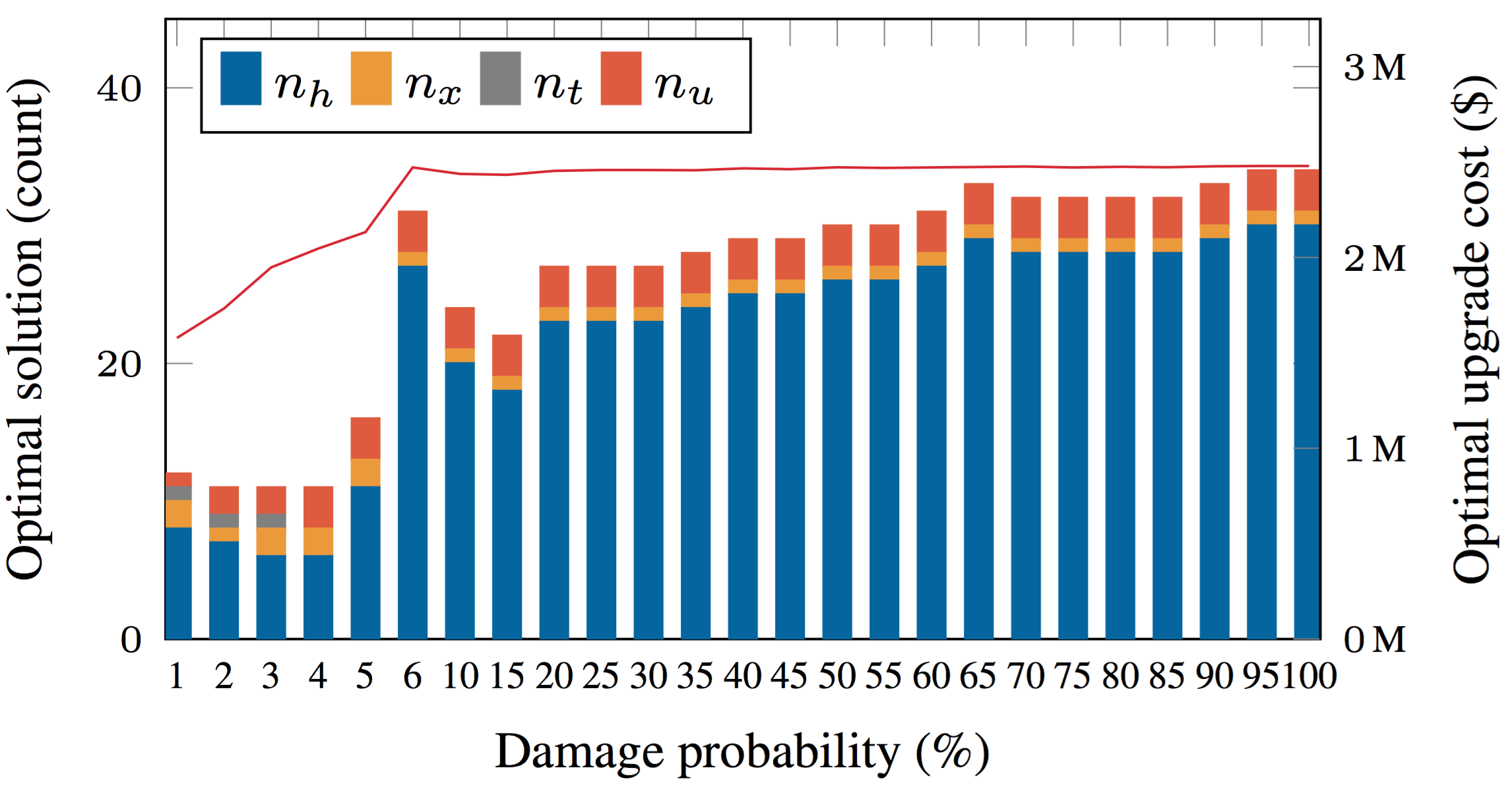
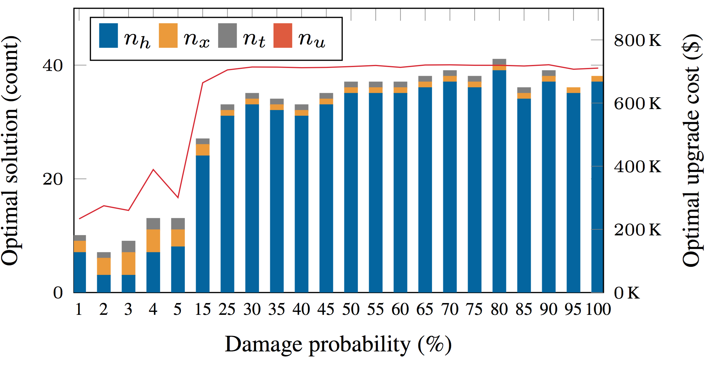
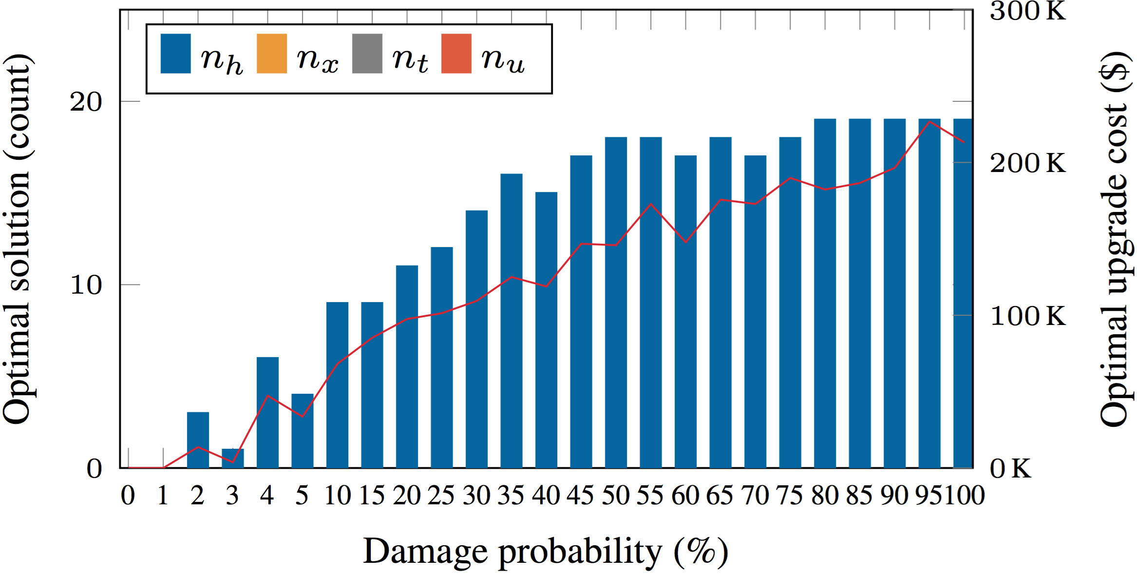
Let $n_{h},n_{x},n_{t},$ and $n_{u}$ be the number of hardened lines, new lines, new switches, and new generators in the optimal design. Figure 6 reports these values for various damage levels and the three networks. The red line indicates the optimal upgrade costs, and the counts of the upgrade options are represented as a bar. The results show that hardening lines is the major component of each optimal design and that its share increases with the disaster intensity. The results also show that DGs are used in significant numbers in the rural network, while new lines and switches complement hardening in the urban model. This was expected given the length of the lines in these two networks. The third network only needs line hardenings.

(a) Rural network

(b) Urban network

(c) Network123

Figure 6: Statistics on the Optimal Grid Designs.

(a) Rural network

(b) Urban network

Figure 7: Optimal Designs of the Rural and Urban Networks (3% damage level).

Figure 8: Optimal Design of Network network123 (20% damage level).

8.2 Impact of the Communication Network

First note that ignoring the communication network is equivalent to assuming that every bus has its own communication center. In the following, $\widetilde{G}(k)$ denotes a communication network with $k$ centers and $\widetilde{G}(\infty)$ the case where each bus has a center.

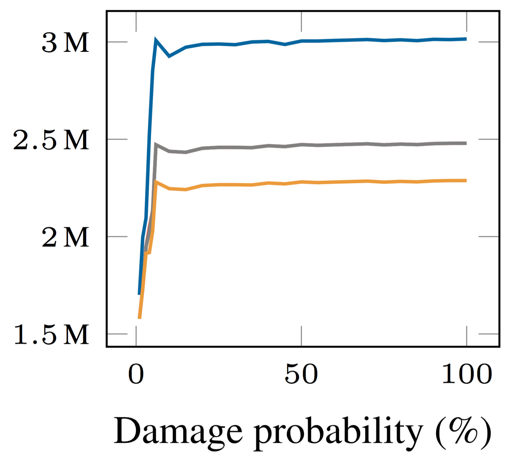
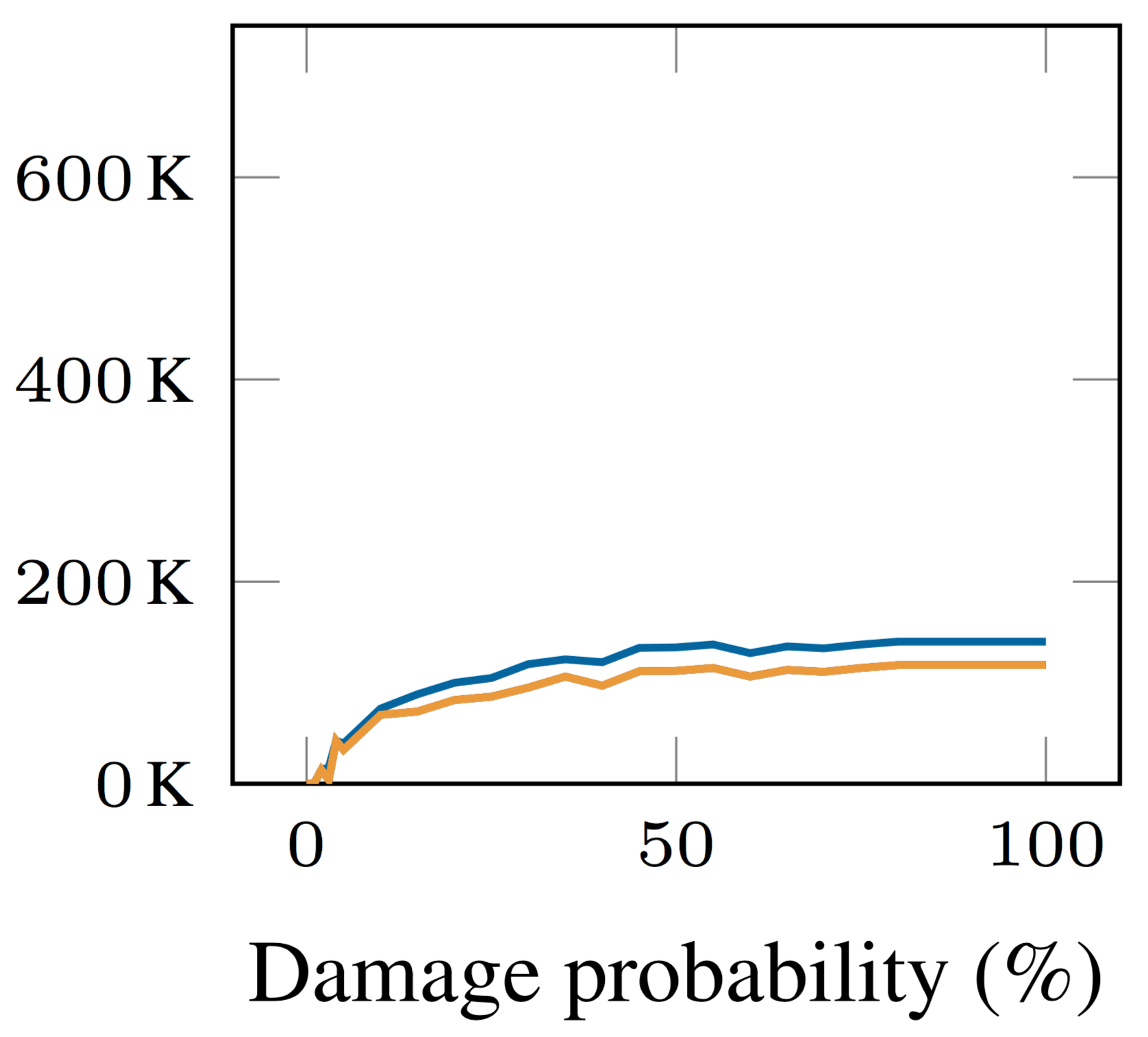
Figure 9 and Table 8.2 report the impact of the communication system: They report optimal objective values and solution statistics under various numbers of communication centers. Fewer communication centers lead to significant cost increases in the rural network, but have limited effect on the urban network and network123. In the rural network, resiliency comes from forming microgrids with DGs, which require their own communication centers. When these are not available, optimal designs harden existing lines and build new lines and switches, which are more costly as substantiated in Table 8.2.

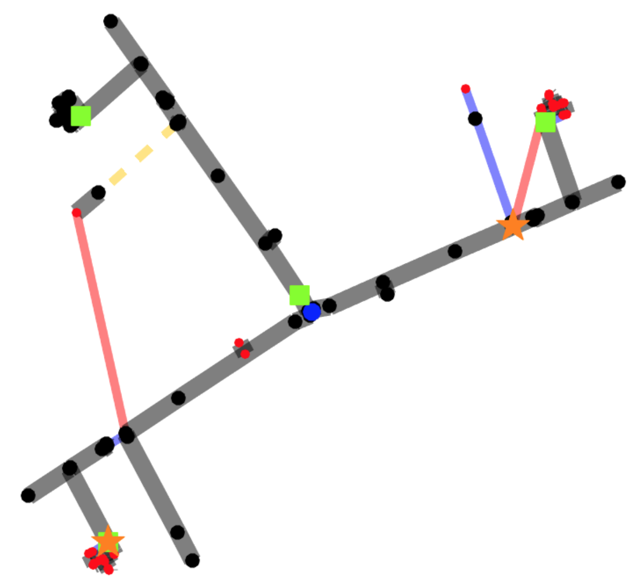
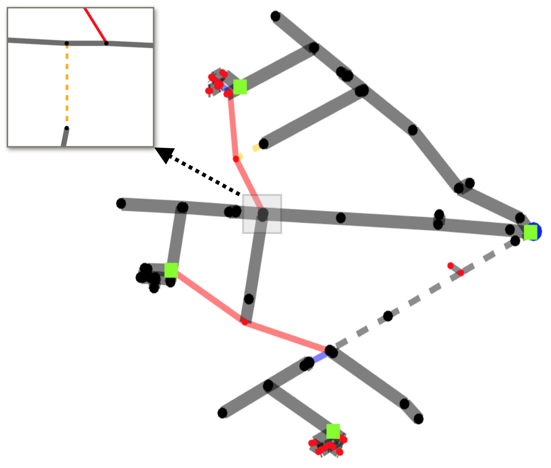
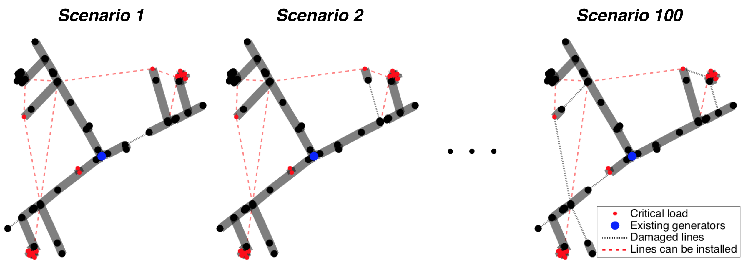
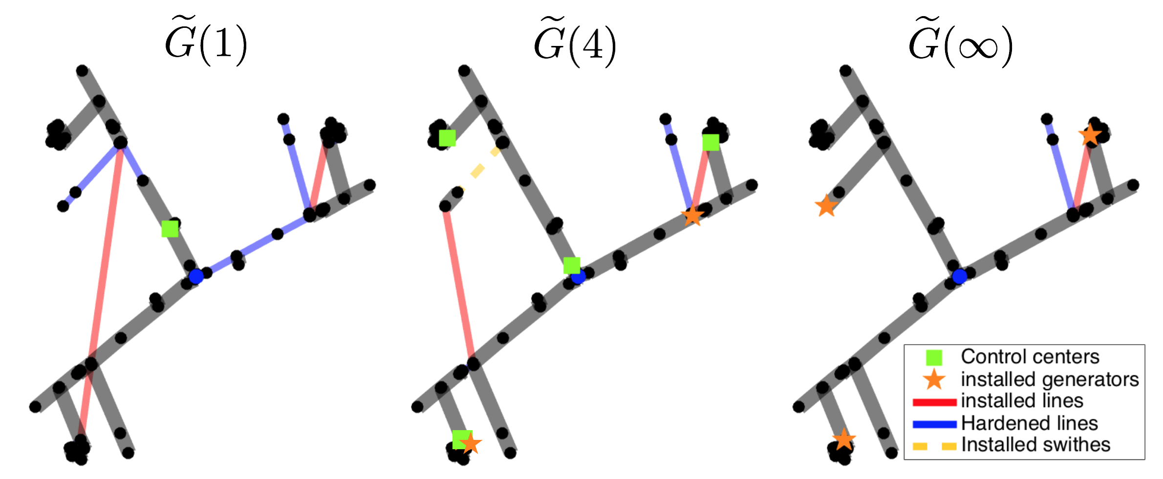
Figure 10 illustrates the resulting designs on the rural network for scenarios with a damage level of 3%. The top row depicts some of the scenarios and shows the affected lines. The bottom row depicts the optimal designs for various configurations of the communication network. For $\widetilde{G}(\infty)$, the optimal design features three new DGs in the west-, north-, and east-end of the network to meet the critical loads of each region. These regions are then islanded under various scenarios. For $\widetilde{G}(4)$, the optimal design installs a new line linking critical loads in the north side to the west side of the network, instead of using DG in the north side. This stems from Scenario 100 where a DG in the bus with critical loads cannot be operated since it has no communication center. For $\widetilde{G}(1)$, scenario 1 prevents the operation of an east-end DG and scenario 100 the operation of a west-end DG. Hence, the optimal design only considers hardening and new lines and switches. On the other hand, the urban network and Network123 achieve resiliency by increasing grid connectivity for all communication networks.

(a) Rural network

(b) Urban network

(c) Network123

Figure 9: Cost Analysis For the Number of Communication Centers

Impact of the Communication Network on Optimal Grid Designs. Comm. Network Obj. $n_{h}$ $n_{x}$ $n_{t}$ $n_{u}$ Rural, 3% damage $\widetilde{G}(1)$ 2095.74 12 3 1 0 $\widetilde{G}(4)$ 1948.09 6 2 1 2 $\widetilde{G}(8)$ 1948.09 6 2 1 2 $\widetilde{G}(\infty)$ 1914.99 5 1 0 3

(a) damage scenarios

(b) Optimal grid design

Figure 10: Optimal Designs of the Rural Network under 3% Damage and Various Communication Network Configurations.

9 Performance Analysis of the Branch and Price Algorithm

This section studies the performance of the B&P algorithm. All computations were implemented with the C++/Gurobi 6.5.2 interface. They use a Haswell architecture compute node configured with 24 cores (two twelve-core 2.5 GHz Intel Xeon E5-2680v3 processors) and 128 GB RAM.

9.1 Computational Performance

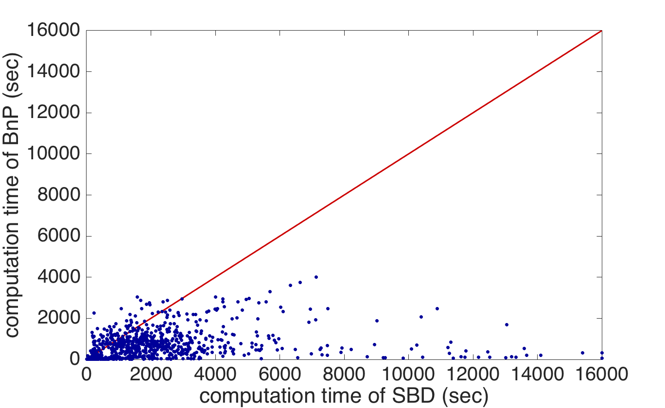
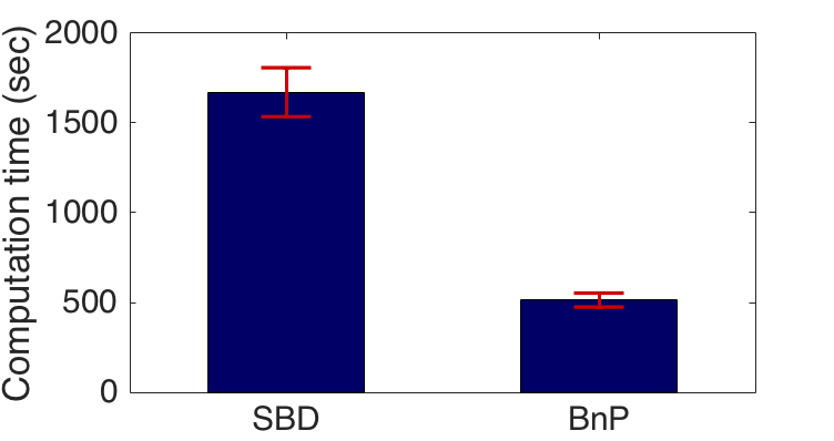
Figure 11a reports the computation time of the B&P and SBD algorithms for all the instances described in Section 7, where the reference line (in red) serves to delineate when an algorithm is faster than the other. Their statistics are displayed in Figure 11b. In average, the B&P algorithm is faster than the SBD algorithm by a factor of 3.25. These figures also indicate that the SBD algorithm has a high degree of performance variance. This comes from the nature of the scenario set $\mathcal{S}$. If $S$ contains a dominating scenario and the scenario has low index in $\mathcal{S}$, then the SBD algorithm solves the problem quickly. Otherwise, the SBD may need a large number of iterations and the MIP model keeps growing in size with each iteration. For 2 out of 1120 instances, the SBD algorithm times out (wallclock time limit of 4 hours). On the other hand, the B&P algorithm is stable across all instances. The B&P algorithm also has the additional benefit that it produces improving feasible solutions continuously. In contrast, the SBD algorithm only produces a feasible solution at optimality. Finally, the B&P algorithm appears more stable numerically than the SBD algorithm. For 5 out of 1120 instances, the B&P algorithm yields a better optimal solution than the SBD algorithm as shown in Table 9.1. Each such solution was validated for feasibility.

(a) Computation Times

(b) Average Computation Times and 95% Confidence Intervals

Figure 11: Comparison of Computation Times: SBD versus B&P.

Numerical Stability of the B&P Algorithm. Instance Opt. obj.val SBD B&P Gap Rural, 30% damage, $\eta_{t}=0.5,$ $\widetilde{G}(4)$ 2458.49 2453.79 -0.19 % Rural, 30% damage, $\eta_{t}=0.6,$ $\widetilde{G}(4)$ 2458.49 2453.79 -0.19 % Rural, 30% damage, $\eta_{t}=0.7,$ $\widetilde{G}(4)$ 2524.68 2519.98 -0.19 % Rural, 30% damage, $\eta_{t}=0.8,$ $\widetilde{G}(4)$ 2572.31 2567.60 -0.19 % Network123, 55% damage, $\eta_{t}=0.8,$ $\widetilde{G}(8)$ 232.48 227.27 -2.24 %

9.2 Solution Quality at the Root Node.

The problem reformulation produces a strong lower bound and the majority of the instances are proven optimal at the root node. Table 9.2 summarizes the average number of branching nodes and the average optimality gap at the root node.

Branching Tree Statistics. Avg. # of branching nodes Avg. opt. gap at the root node 1.8 0.19 %

9.3 Benefits of the Accelerating Schemes

To highlight its design choices, the B&P algorithm is compared to a column generation with dual stabilization (Du Merle et al. 1999). In addition, the benefit of each of the accelerating schemes is investigated independently by running the B&P algorithm without the considered extension. We sample 90 instances by setting $\eta_{t}=0.5$ and $0.8$, and the damage level to $5\%,$ $30\%,$ $65\%,$ $85\%,$ $100\%$ for the three networks $\widetilde{G}(0)$, $\widetilde{G}(1),$ and $\widetilde{G}(4)$. Dual stabilization prevents dual variables from fluctuating too much, which is often the case in column generation. It tries to confine dual variables in a box that contains the current best estimate of the optimal dual solution and penalizes solutions that deviate from the box. See, for instance, Du Merle et al. (1999), Lübbecke and Desrosiers (2005) for details about stabilized column generation. Our implementation updates the box whenever the Lagrangian lower bound is updated.

Table 9.3 summarizes the computational performance of the stabilized column generation in comparison with the B&P algorithm. B&P_B denotes the branch-and-price algorithm with the basic scheme only (Section 6.2) and B&P_S stands for the branch and price algorithm with dual stabilization. The symbol ${\dagger}$ is used to denote that the algorithm reaches the wallclock time limit for some instances. For more than one third of the sampled instances, B&P_B and B&P_S exceed the wallclock time limit. For instances where both algorithms terminate within the time limit, B&P_S is faster than B&P_B by a factor of around 4. Although the dual stabilization does improve the computation time of the basic algorithm, it is still not adequate to solve the ORDPDC practically. The B&P algorithm, on the other hand, shortens computation times by a factor of 26.35.

Comparison to a Column Generation with Dual Stabilization. Avg. computation time (sec) Avg. number of iterations B&P_B 12857.97^† 3122.57^† B&P_S 11563.44^† 1514.58^† B&P 488.03 96.12

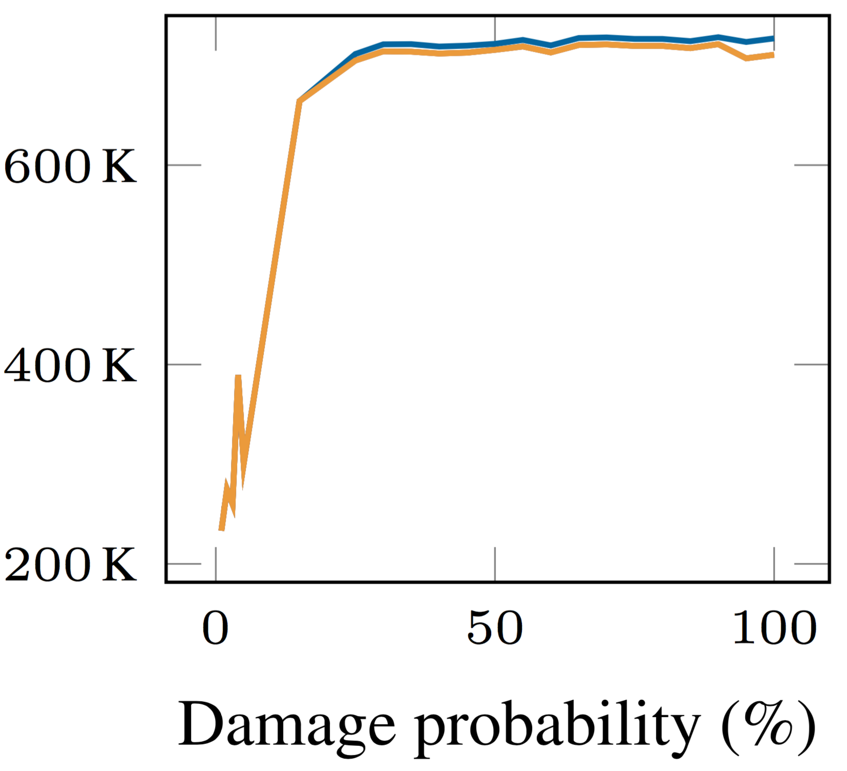
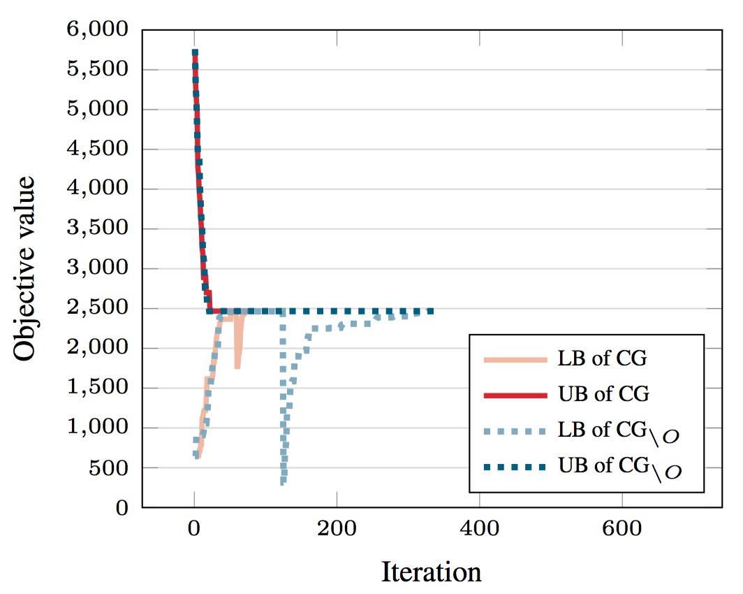
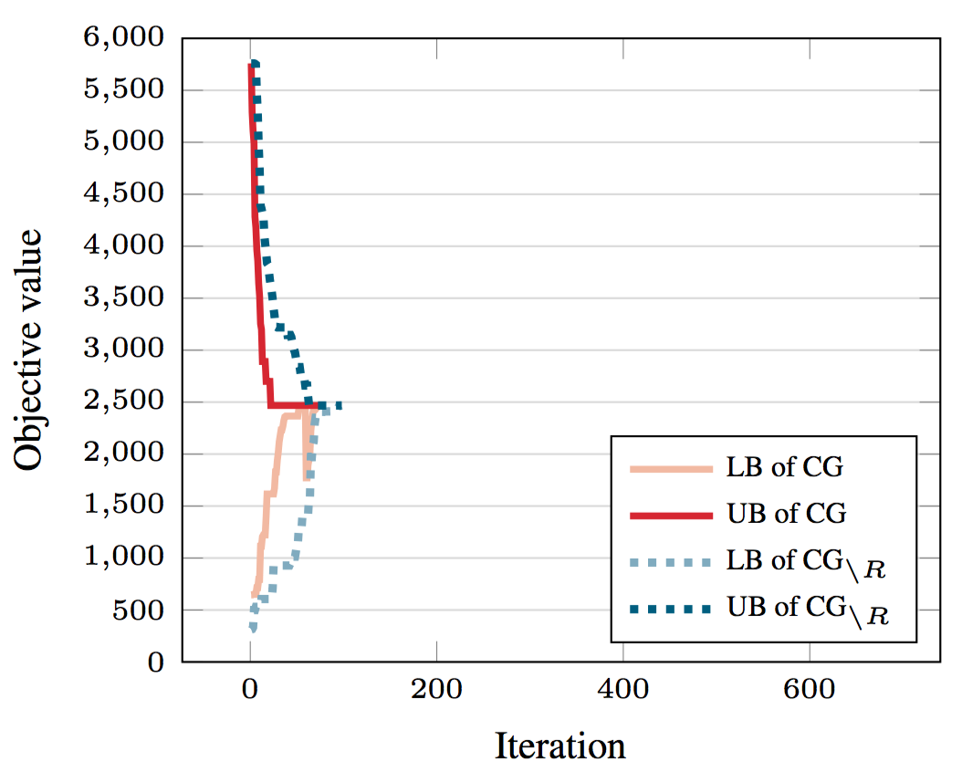
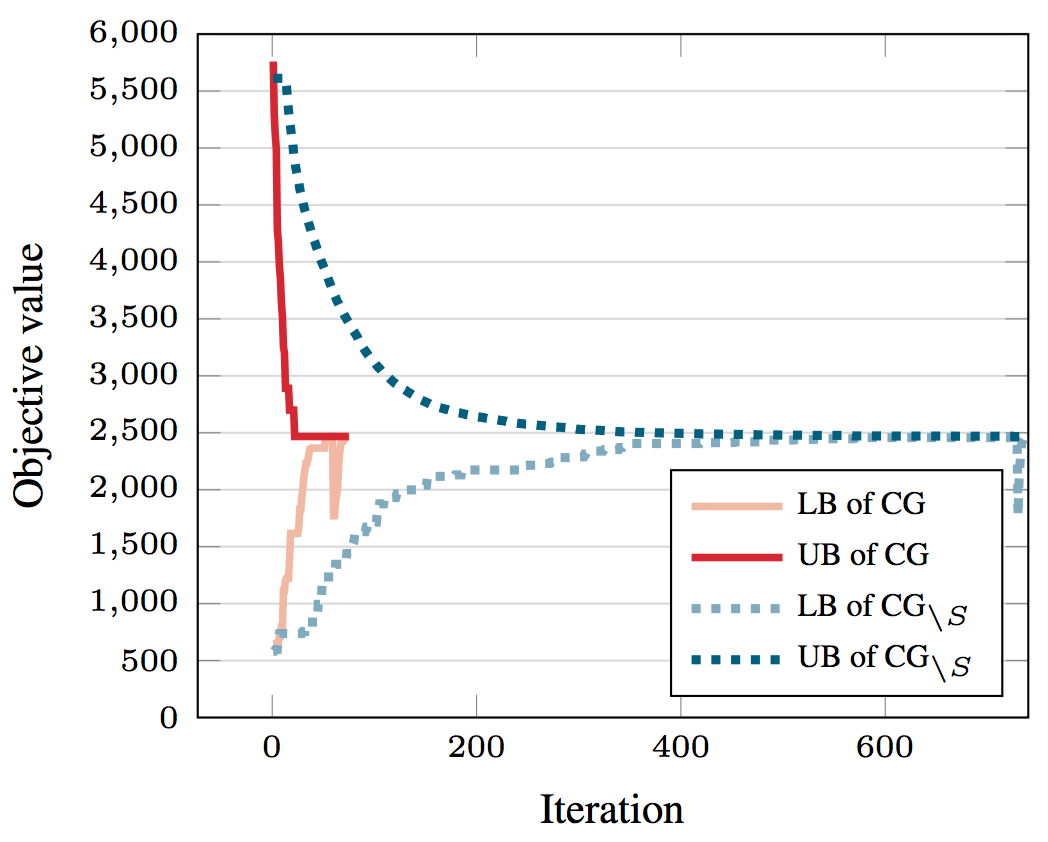
The next results investigate the performance gain of each accelerating scheme by removing them one at a time from the B&P algorithm. Table 9.3 describes the computational performance and Figure 12 illustrates the impact of each accelerating schemes on the convergence rate of the rural network under 6% damage level. In the table and figure, $R$ denotes the revised reduced cost, $C$ the optimality cut, $O$ the lexicographic objective pricing problem, B&P_∖k the B&P algorithm without scheme $k$, with $k\in\{R,C,O\}$, and CG_∖k the column generation of B&P without scheme $k$.

The results in Table 9.3 indicate that all the accelerating schemes contribute to the computational performance of the B&P algorithm. Figure 12a illustrates the key role of the optimality cut. Without this cut, the second stage of the column generation which uses the traditional pricing objective does not take advantage of the columns generated in the first stage and its lower bound drastically drops. Figure 12b compares the convergence behavior of CG and CG_∖R, showing that CG reaches the optimal objective value faster than CG_∖R. Figure 12c highlights the impact of the lexicographic objective function and shows that it significantly contributes to the fast convergence of the algorithm.

Benefits of the Accelerating Schemes. Avg. computation time (sec) Avg. number of iterations B&P 488.03 96.12 B&P_∖R 844.24 96.39 B&P_∖C 2589.55^† 215.94^† B&P_∖O 2979.84^† 544.65^†

(a) Optimality cut

(b) Revised reduced cost

(c) lexicographic objective function

Figure 12: Comparison of Convergence Rates (rural network, 6% level of damage).

10 Conclusions

This paper proposed an expansion planning model to improve the resiliency of distribution systems facing natural disasters. The planning model considers the hardening of existing lines and the addition of new lines, switches, and distributed generators that would allow a subpart of the system to operate as a microgrid. The expansion model uses a 3-phase model of the distribution system. In addition, it also considers damages to the communication system which may prevent generators and switches to be controlled remotely. The input of the expansion model contains a set of damage scenarios, each of which specifying how the disaster affects the distribution system.

The paper proposed a branch and price algorithm for this model where the pricing subproblem generates new expansions for each damage scenario. The branch and price uses a number of acceleration schemes to address significant degeneracy in the model. They include a new pricing objective, an optimality cut, and a multi-objective function to encourage sparsity in the generated expansions. The resulting branch and price algorithm significantly improves the performance of a scenario-based decomposition algorithm and a branch and price with a stabilized column generation. The case studies show that optimal solutions strongly depend on the grid topology and the sophistication of the communication network. In particular, the results highlight the importance of distributed generation for rural networks, which necessitates a resilient communication system.

The acceleration techniques presented in this paper are not limited to the electricity distribution grid planning problem; They can be used on problems with similar structure, i.e, two-stage stochastic problems with feasibility recourse.

Future work will be devoted to applying and scaling these techniques to instances with thousands of components.

References

- Amor et al. (2009) Amor HMB, Desrosiers J, Frangioni A (2009) On the choice of explicit stabilizing terms in column generation. Discrete Applied Mathematics 157(6):1167–1184.
- Barnes et al. (2017) Barnes A, Nagarajan H, Yamangil E, Bent R, Backhaus S (2017) Tools for improving resilience of electric distribution systems with networked microgrids. CoRR abs/1705.08229, URL http://arxiv.org/abs/1705.08229.
- Bialek (2014) Bialek T (2014) Private Communications, San Diego Gas and Electric.
- Carvalho et al. (2005) Carvalho P, Ferreira L, Da Silva AC (2005) A decomposition approach to optimal remote controlled switch allocation in distribution systems. IEEE Transactions on Power Delivery 20(2):1031–1036.
- Chen et al. (2016) Chen C, Wang J, Qiu F, Zhao D (2016) Resilient distribution system by microgrids formation after natural disasters. IEEE Transactions on smart grid 7(2):958–966.
- Ding et al. (2017) Ding T, Lin Y, Li G, Bie Z (2017) A new model for resilient distribution systems by microgrids formation. IEEE Transactions on Power Systems .
- Du Merle et al. (1999) Du Merle O, Villeneuve D, Desrosiers J, Hansen P (1999) Stabilized column generation. Discrete Mathematics 194(1-3):229–237.
- Executive Office of the President (2013) Executive Office of the President (2013) Economic Benefits of Increasing Electric Grid Resilience to Weather Outages. Technical report.
- Falahati et al. (2012) Falahati B, Fu Y, Wu L (2012) Reliability assessment of smart grid considering direct cyber-power interdependencies. IEEE Transactions on Smart Grid 3(3):1515–1524.
- Gan and Low (2014) Gan L, Low SH (2014) Convex relaxations and linear approximation for optimal power flow in multiphase radial networks. Power Systems Computation Conference (PSCC), 2014, 1–9 (IEEE).
- Gao et al. (2016) Gao H, Chen Y, Xu Y, Liu CC (2016) Resilience-Oriented Critical Load Restoration Using Microgrids in Distribution Systems. IEEE Trans. on Smart Grid PP(99):1–1, ISSN 1949-3053, URL http://dx.doi.org/10.1109/TSG.2016.2550625.
- Gholami et al. (2016) Gholami A, Aminifar F, Shahidehpour M (2016) Front lines against the darkness: Enhancing the resilience of the electricity grid through microgrid facilities. IEEE Electrification Magazine 4(1):18–24.
- Kersting (1991) Kersting W (1991) Radial distribution test feeders. IEEE Transactions on Power Systems 6(3):975–985, ISSN 08858950, URL http://dx.doi.org/10.1109/59.119237.
- Lasseter et al. (2002) Lasseter R, Akhil A, Marnay C, Stephens J, Dagle J, Guttromson R, Meliopoulous A, Yinger R, Eto J (2002) The certs microgrid concept. White paper for Transmission Reliability Program, Office of Power Technologies, US Department of Energy 2(3):30.
- Li et al. (2017) Li Z, Shahidehpour M, Aminifar F, Alabdulwahab A, Al-Turki Y (2017) Networked microgrids for enhancing the power system resilience. Proceedings of the IEEE 105(7):1289–1310, ISSN 0018-9219, URL http://dx.doi.org/10.1109/JPROC.2017.2685558.
- Lübbecke and Desrosiers (2005) Lübbecke M, Desrosiers J (2005) Selected topics in column generation. Operations Research 53(6):1007–1023.
- Martins et al. (2017) Martins L, Girao-Silva R, Jorge L, Gomes A, Musumeci F, Rak J (2017) Interdependence between power grids and communication networks: A resilience perspective. DRCN 2017-Design of Reliable Communication Networks; 13th International Conference; Proceedings of, 1–9 (VDE).
- McCormick (1976) McCormick GP (1976) Computability of global solutions to factorable nonconvex programs: Part i—convex underestimating problems. Mathematical programming 10(1):147–175.
- Nagarajan et al. (2016) Nagarajan H, Yamangil E, Bent R, Van Hentenryck P, Backhaus S (2016) Optimal resilient transmission grid design. 2016 Power Systems Computation Conference (PSCC), 1–7 (IEEE).
- Oukil et al. (2007) Oukil A, Amor HB, Desrosiers J, El Gueddari H (2007) Stabilized column generation for highly degenerate multiple-depot vehicle scheduling problems. Computers & Operations Research 34(3):817–834.
- Panteli et al. (2017) Panteli M, Trakas DN, Mancarella P, Hatziargyriou ND (2017) Power systems resilience assessment: Hardening and smart operational enhancement strategies. Proceedings of the IEEE 105(7):1202–1213, ISSN 0018-9219, URL http://dx.doi.org/10.1109/JPROC.2017.2691357.
- Parhizi et al. (2015) Parhizi S, Lotfi H, Khodaei A, Bahramirad S (2015) State of the art in research on microgrids: A review. IEEE Access 3:890–925.
- Resende et al. (2011) Resende F, Gil N, Lopes J (2011) Service restoration on distribution systems using multi-microgrids. International Transactions on Electrical Energy Systems 21(2):1327–1342.
- Sa (2002) Sa Y (2002) Reliability Analysis of Electric Distribution Lines. Ph.D. thesis, McGill University.
- Schrijver (1998) Schrijver A (1998) Theory of linear and integer programming (John Wiley & Sons).
- State of Virginia Corporation Commission (2005) State of Virginia Corporation Commission (2005) Placement of Utility Distribution Lines Underground. Technical Report House Document 30, Governor and the General Assembly of Virginia, Richmond, VA.
- U.S. Energy Information Administration (2014) US Energy Information Administration (2014) Annual Energy Outlook 2014. Technical report, URL http://dx.doi.org/DOE/EIA-0383(2014).
- Wang et al. (2016a) Wang Y, Chen C, Wang J, Baldick R (2016a) Research on resilience of power systems under natural disasters—a review. IEEE Transactions on Power Systems 31(2):1604–1613.
- Wang et al. (2016b) Wang Z, Chen B, Wang J, Chen C (2016b) Networked microgrids for self-healing power systems. IEEE Transactions on smart grid 7(1):310–319.
- Xu et al. (2016) Xu Y, Liu CC, Schneider KP, Ton DT (2016) Placement of remote-controlled switches to enhance distribution system restoration capability. IEEE Transactions on Power Systems 31(2):1139–1150.
- Yamangil et al. (2015) Yamangil E, Bent R, Backhaus S (2015) Resilient upgrade of electrical distribution grids. AAAI, 1233–1240.
- Yuan et al. (2017) Yuan C, Illindala MS, Khalsa AS (2017) Modified viterbi algorithm based distribution system restoration strategy for grid resiliency. IEEE Transactions on Power Delivery 32(1):310–319.
- Yuan et al. (2016) Yuan W, Wang J, Qiu F, Chen C, Kang C, Zeng B (2016) Robust optimization-based resilient distribution network planning against natural disasters. IEEE Transactions on Smart Grid 7(6):2817–2826.