Poisson-Fermi Modeling of Ion Activities in Aqueous Single and Mixed Electrolyte Solutions at Variable Temperature

Abstract. The combinatorial explosion of empirical parameters in tens of thousands presents a tremendous challenge for extended Debye-Hückel models to calculate activity coefficients of aqueous mixtures of most important salts in chemistry. The explosion of parameters originates from the phenomenological extension of the Debye-Hückel theory that does not take steric and correlation effects of ions and water into account. In contrast, the Poisson-Fermi theory developed in recent years treats ions and water molecules as nonuniform hard spheres of any size with interstitial voids and includes ion-water and ion-ion correlations. We present a Poisson-Fermi model and numerical methods for calculating the individual or mean activity coefficient of electrolyte solutions with any arbitrary number of ionic species in a large range of salt concentrations and temperatures. For each activity-concentration curve, we show that the Poisson-Fermi model requires only three unchanging parameters at most to well fit the corresponding experimental data. The three parameters are associated with the Born radius of the solvation energy of an ion in electrolyte solution that changes with salt concentrations in a highly nonlinear manner.

I Introduction

Thermodynamic modeling of aqueous electrolyte solutions plays an important role in chemical and biological sciences RS59 ; N91 ; P95 ; H01 ; LM03 ; F04 ; LJ08 ; KF09 ; K10 ; VW16 ; V11 ; E13 ; RK15 . Despite intense efforts in the past century, robust thermodynamic modeling of electrolyte solutions still presents a difficult challenge and remains a remote ambition in the extended Debye-Hückel (DH) models due to the enormous number of parameters that need to be adjusted, carefully and often subjectively V11 ; RK15 . For example, the Pitzer model requires 8 parameters for a ternary system and up to 8 temperature coefficients (parameters) for every Pitzer parameter in a temperature interval from 0 to about 200 $\operatorname{{}^{\circ}{\rm C}}$ V11 ; RK15 . It is indeed a frustrating despair (frustration on p. 11 in K10 and despair on p. 301 in RS59 ) that approximately 22,000 parameters for combinatorial solutions of the most important 28 cations and 16 anions in salt chemistry have to be extracted from the available experimental data for one temperature V11 . The Pitzer model is still the most widely used DH model with unmatched precision for modeling aqueous electrolyte solutions over wide ranges of composition, temperature, and pressure RK15 .

The Pitzer model and its variants RK15 are all derived from the Debye-Hückel theory DH23 that in turn is based on a linear Poisson-Boltzmann (PB) equation LM03 although potentials calculated from PB near ions (for example) are often far beyond the linear range of the potential near ions or interfaces. The PB equation treats ions as point charges without steric volumes and water molecules as a homogeneous dielectric medium without steric volumes either and with a constant dielectric constant that neglects ion-water and ion-ion correlations. These simplifications give rise to the elegant, simple, and useful DH theory. However, it is precisely because of the linearization and simplifications on steric and correlation effects that extended DH models have needed an explosion in the number of parameters in order to overcome the deficiencies (simplifications) of the classical Poisson-Boltzmann theory. The nonlinear PB equation was developed by Gouy and Chapman G10 ; C13 .

In the past few years, we have intensively investigated these two effects in a range of areas from electric double layers L13 ; LX17 , ion activities LE15a , to biological ion channels LE13 ; LX17 ; LE14 ; LE14a ; LE15 ; LH16 and consequently developed an advanced theory — the Poisson-Fermi (PF) theory — that treats ions and water molecules as nonuniform hard spheres of any size with interstitial voids and includes many of the correlation effects of ions and water. We refer to our previous papers and references therein for a historical account of the literature of this theory. In LE15a , we proposed a PF model for calculating activity coefficients of individual ions in aqueous single NaCl and CaCl₂ electrolyte solutions at the temperature 298.15 K. The model is further tested in this paper for eight 1:1 electrolytes (LiCl, LiBr, NaF, NaCl, NaBr, KF, KCl, and KBr), six 2:1 electrolytes (MgCl₂, MgBr₂, CaCl₂, CaBr₂, BaCl₂, and BaBr₂), one mixed electrolyte (NaCl + MgCl₂), one 1:1 electrolyte (NaCl ) at various temperatures from 298.15 to 573.15 K, and one 2:1 electrolyte (MgCl₂) at various temperatures from 298.15 to 523.15 K, for which the experimental data were compiled by Valiskó and Boda in VB15 and Rowland et al. in RK15 from various experimental sources in WR04 ; PP84 ; BH84 ; A92 ; GN78 ; WP98 ; C09 ; L65 ; KZ24 ; T21 .

The PF model is developed to calculate individual ion activities for which experimental measurements and determination VW16 ; WV05 ; WR06 , interpretation of measurement data WR04 ; WR06 ; WV03 ; WV11 , and comparison of different experimental methods WR06 ; WV16 have been extensively investigated by Wilczek-Vera, Rodil, and Vera in the past two decades. PF results on mean activity coefficients can be compared with experimental measurements using the Debye-Hückel equation of individual ion activities LM03 .

In contrast to the Pitzer model, we show that all experimental data sets of individual or mean activity coefficients as a function of variable concentration in single electrolytes or mixtures at various temperatures can be well fitted by the PF model with only 3 parameters at most for each activity-concentration data curve. The model is characterized by three different domains, namely, the Born ion, hydration shell, and remaining solvent domains in which the Born ion domain is most crucial because all activities around an ion are mainly governed by the singular charge of the ion located at the center of the domain. The Born ion domain is defined by the Born radius of the solvated ion, which is unknown and changes with salt concentrations in a highly nonlinear manner.

The three parameters characterize three orders of approximation of the Born radius in terms of ionic concentrations. Parameter 1 describes a correction of the experimental Born radius of a single ion in pure water without any other ions. Parameter 2 describes an adjustment of the unknown Born radius in electrolyte solution that accounts for the Debye screening effect, which is proportional to the square root of the ionic strength of the solution. Parameter 3 is an adjustment in the next order approximation beyond the DH treatment of ionic atmosphere. The physical origin of these parameters is clear unlike that of most parameters in the Pitzer method F10 ; V11 . It may even be possible in later work to calculate some of these parameters from more detailed versions of our model.

Our approach to partition the free energy domain of a solvated ion into the above three sub-domains yields a better approximation to calculate the free energy since these sub-domains are determined by the experimental data of solvation and thus separate short- and long-range interactions of the ion in a more accurate way. This approach nevertheless incurs more complicated numerical methods for solving the nonlinear partial differential equations of the PF model in different domains with suitable interface conditions L13 . We therefore present numerical methods in detail for future verification and development of the present work.

II Theory

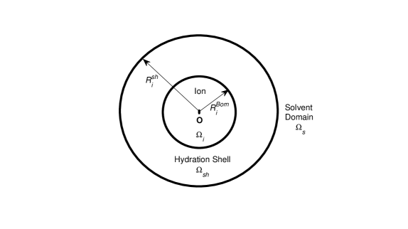
Figure 1: The model domain $\Omega$ is partitioned into the ion domain $\Omega_{i}$ (with radius $R_{i}^{Born}$), the hydration shell domain $\Omega_{sh}$ (with radius $R_{i}^{sh}$), and the remaining solvent domain $\Omega_{s}$.

For an aqueous electrolyte solution with $K$ species of ions, the Poisson-Fermi theory proposed in LX17 ; LE14 treats all ions and water of any diameter as nonuniform hard spheres with interstitial voids between these spheres. The activity coefficient $\gamma_{i}$ of an ion of species $i$ in the solution describes the deviation of the chemical potential of the ion from ideality ($\gamma_{i}=1$). The excess chemical potential $\mu_{i}^{\text{ex}}=k_{B}T\ln\gamma_{i}$ can be calculated by BC00 ; LE15a

$$\mu_{i}^{\text{ex}}=\Delta G_{i}-\Delta G_{i}^{0}\text{, \ }\Delta G_{i}=\frac{1}{2}q_{i}\phi(\mathbf{0})\text{, \ }\Delta G_{i}^{0}=\frac{1}{2}q_{i}\phi^{0}(\mathbf{0})\text{,}$$ (1)

where $k_{B}$ is the Boltzmann constant, $T$ is an absolute temperature, $q_{i}$ is the ionic charge of the hydrated ion (also denoted by $i$), $\phi(\mathbf{r})$ is a potential function of spatial variable $\mathbf{r}$ in the domain $\Omega$ $=$ $\overline{\Omega}_{i}\cup\overline{\Omega}_{sh}\cup\Omega_{s}$ shown in Fig. 1, $\Omega_{i}$ is the spherical domain occupied by the ion $i$, $\Omega_{sh}$ is the hydration shell domain of the ion, $\Omega_{s}$ is the remaining solvent domain, $\mathbf{0}$ denotes the center (set to the origin) of the ion, $\phi(\mathbf{0})$ is the value of $\phi(\mathbf{r})$ at $\mathbf{r}=\mathbf{0}$, and $\phi^{0}(\mathbf{r})$ is a potential function when the solvent domain $\Omega_{s}$ does not contain any ions at all with pure water only. The potential function $\phi(\mathbf{r})$ can be found by solving the Poisson-Fermi equation LX17

$$\left(l_{c}^{2}\nabla^{2}-1\right)\nabla\cdot\epsilon(\mathbf{r})\nabla\phi(\mathbf{r})=\rho(\mathbf{r})\text{,}$$ (2)

$$\epsilon(\mathbf{r}) =\left\{\begin{array}[c]{l}\epsilon_{s}=\epsilon_{\text{w}}\epsilon_{0}\text{ in }\overline{\Omega}_{sh}\cup\Omega_{s}\\ \epsilon_{i}=\epsilon_{\text{ion}}\epsilon_{0}\text{ in }\overline{\Omega}_{i}\end{array}\right.,\text{ }l_{c}=\left\{\begin{array}[c]{l}2a_{j}\text{ in }\overline{\Omega}_{sh}\cup\Omega_{s}\\ 0\text{ in }\overline{\Omega}_{i}\end{array}\right.,$$ (3)

$$\rho(\mathbf{r}) =\left\{\begin{array}[c]{l}\rho_{s}(\mathbf{r})=\sum_{k=1}^{K}q_{k}C_{k}(\mathbf{r})\text{ in }\Omega_{s}\\ 0\text{ in }\overline{\Omega}_{sh}\\ \rho_{i}(\mathbf{r})=q_{i}\delta(\mathbf{r}-\mathbf{0})\text{ in }\overline{\Omega}_{i}\end{array}\right.,$$ (4)

$$C_{k}(\mathbf{r}) =C_{k}^{\text{B}}\exp\left(-\beta_{k}\phi(\mathbf{r})+\frac{v_{k}}{v_{0}}S^{\text{trc}}(\mathbf{r})\right)\text{ in }\overline{\Omega}\text{,}$$ (5)

$$S^{\text{trc}}(\mathbf{r}) =\ln\left(\frac{\Gamma(\mathbf{r)}}{\Gamma^{\text{B}}}\right)\text{ in }\overline{\Omega}\text{,}$$ (6)

where $\epsilon_{0}$ is the vacuum permittivity, $\epsilon_{\text{w}}$ is the dielectric constant of bulk water, $\epsilon_{\text{ion}}$ is a dielectric constant in $\overline{\Omega}_{i}$, $a_{j}$ is the radius of a counterion of the ion $i$, and $\delta(\mathbf{r}-\mathbf{0})$ is the delta function at the origin.

The concentration function $C_{k}(\mathbf{r})$ is described by a Fermi distribution (5), where $C_{k}^{\text{B}}$ is a constant bulk concentration for all $k=1,\cdots,K+1$, $q_{K+1}=0$, $\beta_{k}=q_{k}/k_{B}T$, $v_{k}=4\pi a_{k}^{3}/3$, $v_{0}=\left(\sum_{k=1}^{K+1}v_{k}\right)/(K+1)$ an average volume of all kinds of hard spheres, $S^{\text{trc}}(\mathbf{r})$ is called the steric potential, $\Gamma^{\text{B}}=1-\sum_{k=1}^{K+1}v_{k}C_{k}^{\text{B}}$ is a constant void fraction, $\Gamma(\mathbf{r)}=1-\sum_{k=1}^{K+1}v_{k}C_{k}(\mathbf{r})$ is a void fraction function, and $K+1$ denotes water. The radii of $\Omega_{i}$ and the outer boundary of $\Omega_{sh}$ are denoted by $R_{i}^{Born}$ and $R_{i}^{sh}$, respectively, whose values will be determined by experimental data. It is natural to choose the Born radius $R_{i}^{Born}$ (not the ionic radius $a_{i}$) as the radius of $\Omega_{i}$ BC00 . We consider both first and second shells of the ion RI13 ; MP11 .

The potential $\phi^{0}(\mathbf{r})$ (in Eq. (1)) of the ideal system is obtained by setting $\rho_{s}(\mathbf{r})=0$ in (4), i.e., all particles in $\Omega_{s}$ do not electrostatically interact with each other since $q_{k}=0$ for all $k$. The domain $\Omega$ is chosen to be sufficiently large so that $\phi(\mathbf{r})=0$ on the boundary of the domain $\partial\Omega$. The ideal potential $\phi^{0}(\mathbf{r})$ is then a constant, i.e., $\Delta G_{i}^{0}$ is a constant reference chemical potential independent of $C_{k}^{\text{B}}$.

The distribution (5) is of Fermi type since all concentration functions have an upper bound, i.e., $C_{k}(\mathbf{r})<1/v_{k}$ for all particle species with any arbitrary (or even infinite) potential $\phi(\mathbf{r})$ at any location $\mathbf{r}$ in the domain $\Omega$ LE14 . The Poisson-Fermi equation (2) and the Fermi distribution (5) reduce to the Poisson-Boltzmann equation and the Boltzmann distribution when $l_{c}=S^{\text{trc}}=0$, i.e., when the correlation and steric effects are not considered. The Boltzmann distribution $C_{k}(\mathbf{r})=C_{k}^{\text{B}}\exp\left(-\beta_{k}\phi(\mathbf{r})\right)$ would however diverge if $\phi(\mathbf{r})$ tends to infinity. This is a major deficiency of PB theory for modeling a system with strong local electric fields or interactions E12a . If the correlation length $l_{c}\neq 0$, the dielectric operator $\widehat{\epsilon}=\epsilon_{s}(1-l_{c}^{2}\nabla^{2})$ in Eq. (2) approximates the permittivity of the bulk solvent and the linear response of correlated ions S06 ; BS11 ; L13 ; LE13 , and yields a dielectric function $\widetilde{\epsilon}(\mathbf{r})$ as an output of solving Eq. (2) LE14 . The exact value of $\widetilde{\epsilon}(\mathbf{r})$ at any $\mathbf{r}\in$ $\overline{\Omega}_{sh}\cup\Omega_{s}$ cannot be obtained from Eq. (2) but can be approximated by the simple formula $\widetilde{\epsilon}(\mathbf{r})\approx\epsilon_{i}+$ $C_{\text{H}_{2}\text{O}}(\mathbf{r}\mathbb{)(}\epsilon_{s}-$ $\epsilon_{i})/C_{\text{H}_{2}\text{O}}^{\text{B}}$ since the water density function $C_{\text{H}_{2}\text{O}}(\mathbf{r}\mathbb{)}=C_{K+1}(\mathbf{r}\mathbb{)}$ is an output of Eq. (5). This formula is only for visualizing (approximately) the profile of $\widehat{\epsilon}$ or $\widetilde{\epsilon}$. It is not an input of calculation. The input is the correlation length $l_{c}$ in Eq. (3) S06 ; BS11 ; L13 ; LE13 . The actual outputs are the numerical solutions of the partial differential equations and boundary conditions.

The factor $v_{k}/v_{0}$ multiplying the steric potential function $S^{\text{trc}}(\mathbf{r})$ in Eq. (5) is a modification of the unity used in our previous work LE14 ; LE15a . The steric energy $-\frac{v_{k}}{v_{0}}S^{\text{trc}}(\mathbf{r})k_{B}T$ LE14 ; LH16 of a type $k$ particle depends not only on the voidness ($\Gamma(\mathbf{r)}$) (or equivalently crowding) at $\mathbf{r}$ but also on the volume $v_{k}$ of the particle itself. If all $v_{k}$ are equal (and thus $v_{k}=v_{0}$), then all particle species at any location $\mathbf{r}\in\overline{\Omega}_{sh}\cup\Omega_{s}$ have the same steric energy, i.e., uniform particles are indistinguishable in steric energy. The steric potential is a mean-field approximation of Lennard-Jones (L-J) potentials that describe local variations of L-J distances (and thus empty voids) between any pair of particles. L-J potentials are highly oscillatory and extremely expensive and unstable to compute numerically LE14 . Calculations that involve L-J potentials, or even truncated versions of L-J potentials must be extensively checked to be sure that results do not depend on irrelevant parameters.

III Methods

To avoid large errors in approximation caused by the delta function $\delta(\mathbf{r}-\mathbf{0})$ in (4), the potential function can be decomposed as CL03 ; GY07 ; L13

$$\phi(\mathbf{r})=\left\{\begin{array}[c]{l}\widetilde{\phi}(\mathbf{r})+\phi^{\ast}(\mathbf{r})+\phi^{\text{L}}(\mathbf{r})\text{\ in }\Omega_{i}\\ \widetilde{\phi}(\mathbf{r})\text{ in }\overline{\Omega}_{sh}\cup\Omega_{s}\end{array}\right.\text{,}$$ (7)

where $\phi^{\ast}(\mathbf{r})=q_{i}/(4\pi\epsilon_{i}\left|\mathbf{r-0}\right|)$ and $\widetilde{\phi}(\mathbf{r})$ is found by solving

$$\left(l_{c}^{2}\nabla^{2}-1\right)\nabla\cdot\epsilon_{s}\nabla\widetilde{\phi}(\mathbf{r}) =\rho(\mathbf{r})\text{ in }\overline{\Omega}_{sh}\cup\Omega_{s}$$ (8)

$$-\nabla\cdot\epsilon_{i}\nabla\widetilde{\phi}(\mathbf{r}) =0\text{ \ in }\Omega_{i}$$ (9)

without the singular source term $\rho_{i}(\mathbf{r})=q_{i}\delta(\mathbf{r}-\mathbf{0})$ and with the interface conditions

$$\left\{\begin{array}[c]{l}\left[\widetilde{\phi}(\mathbf{r})\right]=0\\ \left[\epsilon(\mathbf{r})\nabla\widetilde{\phi}(\mathbf{r})\cdot\mathbf{n}\right]=\epsilon_{i}\nabla\left(\phi^{\ast}(\mathbf{r})+\phi^{\text{L}}(\mathbf{r}))\right)\cdot\mathbf{n}\end{array}\right.\text{ for all }\mathbf{r}\in\partial\Omega_{i}\text{,}$$ (10)

where $\mathbf{n}$ is an outward normal unit vector at $\mathbf{r}\in$ $\partial\Omega_{i}$ and the jump function $[u(\mathbf{r})]=\lim_{\mathbf{r}_{sh}\rightarrow\mathbf{r}}u(\mathbf{r}_{sh})-\lim_{\mathbf{r}_{i}\rightarrow\mathbf{r}}u(\mathbf{r}_{i})$ with $\mathbf{r}_{sh}\in$ $\Omega_{sh}$ and $\mathbf{r}_{i}\in$ $\Omega_{i}$ L13 . The potential function $\phi^{\text{L}}(\mathbf{r})$ is the solution of the Laplace equation

$$\nabla^{2}\phi^{\text{L}}(\mathbf{r})=0\text{ in }\Omega_{i}$$ (11)

with the boundary condition

$$\phi^{\text{L}}(\mathbf{r})=\phi^{\ast}(\mathbf{r})\text{ on }\partial\Omega_{i}.$$ (12)

The evaluation of the Green’s function $\phi^{\ast}(\mathbf{r})$ on $\partial\Omega_{i}$ always yields finite numbers and thus avoids the singularity in the solution process. The desired solvation energy $\Delta G_{i}$ in Eq. (1) (and thus the individual ionic activity coefficient $\gamma_{i}$) is then evaluated by GY07 ; L13

$$\Delta G_{i}=k_{B}T\ln\gamma_{i}=\frac{1}{2}q_{i}\left[\widetilde{\phi}(\mathbf{0})+\phi^{\text{L}}(\mathbf{0})\right]\text{.}$$ (13)

Since the interface $\partial\Omega_{i}$ is a sphere centered at the origin, the Laplace potential $\phi^{\text{L}}(\mathbf{r})=q_{i}/(4\pi\epsilon_{i}R_{i}^{Born})$ is a constant in $\overline{\Omega}_{i}$, i.e., Eq. (11) has been exactly solved.

The Poisson-Fermi equation (8) is a nonlinear fourth-order partial differential equation (PDE) in $\Omega_{s}$. Newton’s iterative method is usually used for solving nonlinear problems. We seek a sequence of approximate solutions $\left\{\widetilde{\phi}_{m}(\mathbf{r})\right\}_{m=1}^{M}$ by iteratively solving the linearized PF equation

$$\left(l_{c}^{2}\nabla^{2}-1\right)\nabla\cdot\epsilon\nabla\widetilde{\phi}_{m}-\rho_{s}^{\prime}(\widetilde{\phi}_{m-1})\text{ }\widetilde{\phi}_{m}=\rho_{s}(\widetilde{\phi}_{m-1})-\rho_{s}^{\prime}(\widetilde{\phi}_{m-1})\text{ }\widetilde{\phi}_{m-1}\text{ in }\Omega_{s}\text{,}$$ (14)

until a tolerable potential function $\widetilde{\phi}_{M}$ is reached, where $\widetilde{\phi}_{0}(\mathbf{r})$ is a given initial guess potential function, $\rho_{s}(\widetilde{\phi}_{m-1})=\sum_{k=1}^{K}q_{k}C_{k}^{m-1}(\mathbf{r})$, $C_{k}^{m-1}(\mathbf{r})=C_{k}^{\text{B}}\exp\left(-\beta_{k}\widetilde{\phi}_{m-1}(\mathbf{r})+\frac{v_{k}}{v_{0}}S_{m-1}^{\text{trc}}(\mathbf{r})\right)$, $S_{m-1}^{\text{trc}}(\mathbf{r})=\ln\left(\frac{\Gamma_{0}(\mathbf{r)}}{\Gamma^{\text{B}}}\right)$, $\Gamma_{m-1}(\mathbf{r)}=1-\sum_{k=1}^{K+1}v_{k}C_{k}^{m-1}(\mathbf{r})$, $\rho_{s}^{\prime}(\widetilde{\phi}_{m-1})=\sum_{k=1}^{K}\left(-\beta_{k}q_{k}\right)C_{k}^{m-1}(\mathbf{r})$, and $\rho_{s}^{\prime}(\widetilde{\phi})=\frac{d}{d\widetilde{\phi}}\rho_{s}(\widetilde{\phi})$. Note that the differentiation in $\rho_{s}^{\prime}(\widetilde{\phi})$ is performed only with respect to $\widetilde{\phi}$ whereas $S^{\text{trc}}$ is treated as another independent variable although $S^{\text{trc}}$ depends on $\widetilde{\phi}$ as well. Therefore, $\rho_{s}^{\prime}(\widetilde{\phi})$ is not exact implying that this is an inexact Newton’s method DE82 .

The fourth-order problem can be resolved by transforming Eq. (14) into two second-order PDEs L13

$$\epsilon_{s}\left(l_{c}^{2}\nabla^{2}-1\right)\Psi(\mathbf{r}) =\rho(\widetilde{\phi}_{m-1})\text{ in }\overline{\Omega}_{sh}\cup\Omega_{s}$$ (15)

$$-\epsilon_{s}\nabla^{2}\widetilde{\phi}_{m}(\mathbf{r})-\rho^{\prime}(\widetilde{\phi}_{m-1})\text{ }\widetilde{\phi}_{m}(\mathbf{r}) =-\epsilon_{s}\Psi(\mathbf{r})-\rho^{\prime}(\widetilde{\phi}_{m-1})\text{ }\widetilde{\phi}_{m-1}\text{ in }\overline{\Omega}_{sh}\cup\Omega_{s}$$ (16)

by introducing a density like variable $\Psi=\nabla^{2}$ $\widetilde{\phi}$ for which the boundary condition is L13

$$\Psi(\mathbf{r})=0\text{ on }\partial\Omega_{s}\text{.}$$ (17)

Eqs. (9), (15), and (16) are coupled together in the entire domain $\Omega$ with the jump conditions in (10). Note that linear PDEs (14), (15), and (16) converge to the nonlinear PDE (8) if $\widetilde{\phi}_{M}$ converges to the exact solution $\widetilde{\phi}$ of Eq. (8) as $M\rightarrow\infty$, i.e., the approximate potential $\widetilde{\phi}_{M}(\mathbf{r})$ is sufficiently close to the exact potential $\widetilde{\phi}(\mathbf{r})$ for all $\mathbf{r}\in$ $\overline{\Omega}_{sh}\cup\Omega_{s}$ if the iteration number $M$ is sufficiently large ($M\approx 5$ to $37$ for this work with error tolerance 10^-3).

The standard 7-point finite difference (FD) method is used to discretize all PDEs (9), (15), and (16), where the jump conditions in (10) are handled by the simplified matched interface and boundary (SMIB) method proposed in L13 . For simplicity, the SMIB method is illustrated by the following 1D linear Poisson equation (in $x$-axis)

$$-\frac{d}{dx}\left[\epsilon(x)\frac{d}{dx}\widetilde{\phi}(x)\right]=f(x)\text{ in }\Omega$$ (18)

with the jump condition

$$\left[\epsilon\widetilde{\phi}^{\prime}\right]=-\epsilon_{i}\frac{d}{dx}\phi^{\ast}(x)\text{ at }x=\xi=\text{ }\partial\Omega_{i}\cap\partial\Omega_{s}\text{,}$$ (19)

where $\Omega=$ $\Omega_{i}\cup\Omega_{s}$, $\Omega_{i}=(0,$ $\xi)$, $\Omega_{s}=(\xi,$ $L)$, $f(x)=0$ in $\Omega_{i}$, $f(x)\neq 0$ in $\Omega_{s}$, and $\widetilde{\phi}^{\prime}=\frac{d}{dx}\widetilde{\phi}(x)$. The corresponding cases to Eqs. (9), (15), and (16) in $y$- and $z$-axis follow in a similar way. Let two FD grids points $x_{l}$ and $x_{l+1}$ across the interface point $\xi$ be such that $x_{l}<\xi<x_{l+1}$ and $\xi=(x_{l}+x_{l+1})/2$ with $\Delta x=x_{l+1}-x_{l}=1$ Å, a uniform mesh, for example, as used in this work. The FD equations of the SMIB method at $x_{l}$ and $x_{l+1}$ are

$$\epsilon_{i}\frac{-\widetilde{\phi}_{l-1}+(2-c_{1})\widetilde{\phi}_{l}-c_{2}\widetilde{\phi}_{l+1}}{\Delta x^{2}} =f_{l}+\frac{c_{0}}{\Delta x^{2}}$$ (20)

$$\epsilon_{s}\frac{-d_{1}\widetilde{\phi}_{l}+(2-d_{2})\widetilde{\phi}_{l+1}-\widetilde{\phi}_{l+2}}{\Delta x^{2}} =f_{l+1}+\frac{d_{0}}{\Delta x^{2}},$$ (21)

where

$$c_{1} =\frac{\epsilon_{i}-\epsilon_{s}}{\epsilon_{i}+\epsilon_{s}}\text{, }c_{2}=\frac{2\epsilon_{s}}{\epsilon_{i}+\epsilon_{s}}\text{, }c_{0}=\frac{-\epsilon_{i}\Delta x\left[\epsilon\widetilde{\phi}^{\prime}\right]}{\epsilon_{i}+\epsilon_{s}}\text{, }$$

$$d_{1} =\frac{2\epsilon_{i}}{\epsilon_{i}+\epsilon_{s}}\text{, }d_{2}=\frac{\epsilon_{s}-\epsilon_{i}}{\epsilon_{i}+\epsilon_{s}}\text{, }d_{0}=\frac{-\epsilon_{s}\Delta x\left[\epsilon\widetilde{\phi}^{\prime}\right]}{\epsilon_{i}+\epsilon_{s}}\text{,}$$

$\widetilde{\phi}_{l}$ is an approximation of $\widetilde{\phi}(x_{l})$, and $f_{l}=f(x_{l})$. Note that the jump value $\left[\epsilon\widetilde{\phi}^{\prime}\right]$ at $\xi$ is calculated exactly since the derivative of $\phi^{\ast}$ is given analytically.

Since the steric potential takes particle volumes and voids into account, the shell volume $V_{sh}$ of the shell domain $\Omega_{sh}$ can be determined by Eqs. (5) and (6) as

$$S_{sh}^{\text{trc}}=\frac{v_{0}}{v_{\text{w}}}\ln\left(\frac{O_{i}^{\text{w}}}{V_{sh}C_{K+1}^{\text{B}}}\right)=\ln\left(\frac{V_{sh}-v_{\text{w}}O_{i}^{\text{w}}}{V_{sh}\Gamma^{\text{B}}}\right)\text{,}$$ (22)

where the occupancy (coordination) number $O_{i}^{\text{w}}$ is given by experimental data RI13 ; MP11 . The shell radius $R_{i}^{sh}$ of $\Omega_{sh}$ is thus determined. Note that the shell volume depends not only on $O_{i}^{\text{w}}$ but also on the bulk void fraction $\Gamma^{\text{B}}$, namely, on all salt and water concentrations ($C_{k}^{\text{B}}$).

As discussed in VB15 , the solvation free energy of an ion $i$ should vary with salt concentrations and can be expressed by a dielectric constant $\epsilon(C_{i}^{\text{B}})$ that depends on the bulk concentration $C_{i}^{\text{B}}$ of the ion. Therefore, the Born energy

$$\Delta G_{i}^{\text{Born}}=\left(\frac{1}{\epsilon_{\text{w}}}-1\right)\frac{q_{i}^{2}}{8\pi\epsilon_{0}R_{i}^{0}}$$ (23)

with the Born radius $R_{i}^{0}$ in pure water should be modified with the concentration-dependent dielectric constant $\epsilon(C_{i}^{\text{B}})$. Equivalently, the Born radius in electrolyte solutions can be modified from $R_{i}^{0}$ by a simple formula

$$R_{i}^{Born}(C_{i}^{\text{B}})=\theta(C_{i}^{\text{B}})R_{i}^{0}\text{, \ \ }\theta(C_{i}^{\text{B}})=\alpha_{1}^{i}+\alpha_{2}^{i}\left(\overline{C}_{i}^{\text{B}}\right)^{1/2}+\alpha_{3}^{i}\left(\overline{C}_{i}^{\text{B}}\right)^{3/2}\text{,}$$ (24)

where $\overline{C}_{i}^{\text{B}}=$ $C_{i}^{\text{B}}$/M is a dimensionless bulk concentration of type $i$ ions, M is the molar concentration unit, and $\alpha_{1}^{i}$, $\alpha_{2}^{i}$, and $\alpha_{3}^{i}$ are adjustable parameters for modifying the experimental Born radius $R_{i}^{0}$ to fit experimental activity coefficients $\gamma_{i}$ that change with the bulk concentration conditions $C_{i}^{\text{B}}$ of the ion. The Born radii $R_{i}^{0}$ in Table 1 are cited from VB15 , which are computed from the experimental hydration Helmholtz free energies of these ions given in F04 . Numerical values in Tables 1 and 2 are all experimental data for which their values are kept fixed throughout calculations once chosen.

The three parameters in Eq. (24) have physical or mathematical meanings unlike many parameters in the Pitzer model F10 . Any model or numerical method incurs errors to approximate a real system, i.e., it is impossible to obtain real Born radius $R_{i}^{Born}(C_{i}^{\text{B}})$ exactly. The first parameter $\alpha_{1}^{i}$ is an adjustment of the experimental Born radius $R_{i}^{0}$ when $C_{i}^{\text{B}}=0$ for all $i$. The second parameter $\alpha_{2}^{i}$ is an adjustment of $R_{i}^{Born}(C_{i}^{\text{B}})$ that accounts for the real thickness of the ionic atmosphere (Debye length), which is proportional to the square root of the ionic strength $\sqrt{I}$ in the Debye-Hückel theory LM03 . The third parameter $\alpha_{3}^{i}$ is simply an adjustment in the next order approximation beyond the DH treatment of ionic atmosphere.

We summarize the mathematical solution process for determining the activity of ionic solutions in the following algorithm.

$\left.\begin{array}[c]{l}\text{1. Solve Eqs. (9), (10), and (16) for }\widetilde{\phi}\text{ with }\rho^{\prime}=\Psi=0\text{ (in pure water), }R_{i}^{Born}=R_{i}^{0}\text{,}\\ \text{ }\ \ \ \text{and }\phi^{\text{L}}=q_{i}/(4\pi\epsilon_{i}R_{i}^{0})\text{ to obtain }\Delta G_{i}^{0}\text{ by Eq. (13) and then set }\widetilde{\phi}_{0}=\widetilde{\phi}\text{.}\\ \text{2. Solve Eqs. (15) and (17) for }\Psi\text{ with }R_{i}^{Born}\text{ in (24).}\\ \text{3. Solve Eqs. (9), (10), and (16) for }\widetilde{\phi}_{m}\text{ with }\phi^{\text{L}}=q_{i}/(4\pi\epsilon_{i}R_{i}^{Born})\text{ and then set }\widetilde{\phi}_{m-1}=\widetilde{\phi}_{m}\text{. }\\ \text{ \ \ \ Go to 2 until convergence. }\\ \text{4. Obtain the activity coefficient }\gamma_{i}\text{ by Eq. (13).}\end{array}\text{ }\right.$

Table 1. Values of Model Notations Symbol Meaning  Value  Unit $k_{B}$ Boltzmann constant $1.38\times 10^{-23}$ J/K $T$ temperature Table 2 K $e$ proton charge $1.602\times 10^{-19}$ C $\epsilon_{0}$ permittivity of vacuum $8.85\times 10^{-14}$ F/cm $\epsilon_{\text{ion}}$, $\epsilon_{\text{w}}$ dielectric constants $1$, Table 2 $l_{c}=2a_{j}$ correlation length $j=\text{Cl}^{-}$ etc. Å $O_{i}^{\text{w}}$ in Eq. (22) 18 RI13 ; MP11 $a_{\text{Li}^{+}}$, $a_{\text{Na}^{+}}$, $a_{\text{K}^{+}}$ radii $0.6$, $0.95$, $1.33$ Å $a_{\text{Mg}^{2+}}$, $a_{\text{Ca}^{2+}}$, $a_{\text{Ba}^{2+}}$ radii $0.65$, $0.99$, $1.35$ Å $a_{\text{F}^{-}}$,$a_{\text{Cl}^{-}}$, $a_{\text{Br}^{-}}$, $a_{\text{H}_{2}\text{O}}$ radii $1.36$, $1.81$, $1.95$, $1.4$ Å $R_{\text{Li}^{+}}^{0}$, $R_{\text{Na}^{+}}^{0}$, $R_{\text{K}^{+}}^{0}$ Born radii in Eq. (24) $1.3$, $1.618$, $1.95$ Å $R_{\text{Mg}^{2+}}^{0}$, $R_{\text{Ca}^{2+}}^{0}$, $R_{\text{Ba}^{2+}}^{0}$ Born radii $1.424$, $1.708$, $2.03$ Å $R_{\text{Cl}^{-}}^{0}$, $R_{\text{Cl}^{-}}^{0}$, $R_{\text{Cl}^{-}}^{0}$, Born radii $1.6$, $2.266$, $2.47$ Å

Table 2. Values of $\epsilon_{\text{w}}$ at various $T$ FG97 . $T$/K 298.15 373.15 423.15 473.15 523.15 573.15 $\epsilon_{\text{w}}$ 78.41 55.51 44.04 38.23 32.23 25.07

IV Results

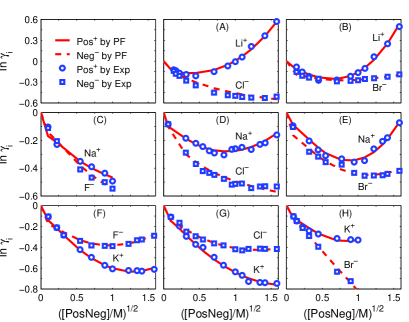
Figure 2: Indivivual activity coefficients of 1:1 electrolytes. Comparison of PF results with experimental data WR04 on $i=$ Pos⁺ (cation) and Neg^- (anion) activity coefficients $\gamma_{i}$ in various [PosNeg] from 0 to 1.6 M.

The PF results of ionic activity coefficients for eight 1:1 electrolytes, six 2:1 electrolytes, one mixed electrolyte, one 1:1 electrolyte at various temperatures, and one 2:1 electrolyte at various temperatures agree with the experimental data WR04 ; PP84 ; BH84 ; A92 ; GN78 ; WP98 ; C09 ; L65 ; KZ24 ; T21 as shown in Figs. 2, 3, 4, 5, and 6, respectively. The empirical parameters used to fit the experimental data are $\alpha_{1}^{i}$, $\alpha_{2}^{i}$, and $\alpha_{3}^{i}$ in Eq. (24), whose values are given in Table 3 from which we observe that the PF model requires only one to three parameters to fit those data.

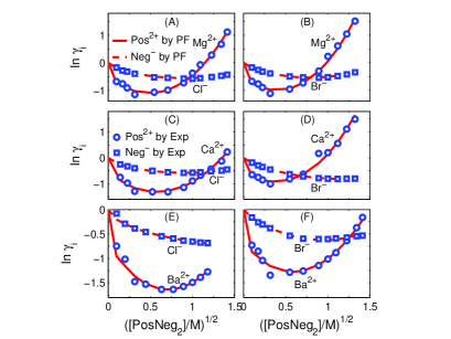
Figure 3: Indivivual activity coefficients of 2:1 electrolytes. Comparison of PF results with experimental data WR04 on $i=$ Pos²⁺ (cation) and Neg^- (anion) activity coefficients $\gamma_{i}$ in various [PosNeg₂] from 0 to 1.5 M.

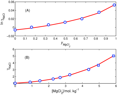
Figure 4: Mean activity coefficients of mixed electrolytes. Comparison of PF results (curve) with experimental data (symbols) compiled in RK15 (A) from L65 on mean activity coefficients $\gamma$ of NaCl as a function of the ionic strength ($I$) fraction $y_{\text{MgCl}_{2}}$of MgCl₂ in NaCl + MgCl₂ mixtures at $I=$ 6 mol. kg^-1 and $T=$ 298.15 K; (B) from KZ24 (circles) and T21 (squares) on $\gamma$ of NaCl as a function of the MgCl₂ molality in NaCl + MgCl₂ mixtures at [NaCl] $=$ 6 mol. kg^-1 and $T=$ 298.15 K.

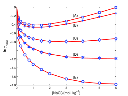
Figure 5: Mean activity coefficients of 1:1 electrolyte at various temperatures. Comparison of PF results (curves) with experimental data (symbols) compiled in RK15 from PP84 ; BH84 ; A92 on mean activity coefficients $\gamma$ of NaCl in [NaCl] from 0 to 6 mol. kg^-1 at $T=$ (A) 298.15 (B) 373.15 (C) 473.15 (D) 523.15 (E) 573.15 K.

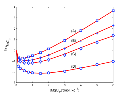
Figure 6: Mean activity coefficients of 2:1 electrolyte at various temperatures. Comparison of PF results (curves) with experimental data (symbols) compiled in RK15 from GN78 ; WP98 ; C09 on mean activity coefficients $\gamma$ of MgCl₂ in [MgCl₂] from 0 to 6 mol. kg^-1 at $T=$ (A) 298.15 (B) 373.15 (C) 423.15 (D) 523.15 K.

The mean activity coefficient $\gamma_{PosNeg}$ of a salt Pos_pNeg_q is calculated via the formula $\ln\gamma_{PosNeg}=\frac{p}{p+q}\ln\gamma_{Pos}+\frac{q}{p+q}\ln\gamma_{Neg}$ LM03 , where $\gamma_{Pos}$ and $\gamma_{Neg}$ are individual activity coefficients obtained by Eq. (13) for each $i=Pos$ and $Neg$. For the mean activity coefficients of either ternary (Fig. 4) or binary (Figs. 5 and 6) systems, we only need to adjust 3 parameters of one cation (not all ions) as shown in Table 3.

The activity coefficients by the PF model are quite successful over a large range of temperatures and concentrations as shown in Figs. 4-6. We used the code of the density model developed by Mao and Duan MD08 to convert the concentration unit from molality (mol. kg^-1) to molarity (M = mol. dm^-3) by the standard formula as given in MD08 , where the density model has been compared with thousands of measurements at high accuracy. The pressure values needed in the code at the corresponding temperatures were set to $P=$ (A) 1.01 (B) 1.01 (C) 15.48 (D) 39.59 (E) 80.50 bar for Fig. 4 and (A) 1.01 (B) 1.01 (C) 4.73 (D) 39.50 bar for Fig. 5. In Fig. 6, the ionic strength $I=\sum_{i}C_{i}^{\text{B}}z_{i}^{2}$ and the ionic strength fraction $y_{\text{MgCl}_{2}}=$ $3m_{\text{MgCl}_{2}}/(3m_{\text{MgCl}_{2}}+m_{\text{NaCl}})$ with $m_{\text{MgCl}_{2}}$ and $m_{\text{NaCl}}$ being the molalities of MgCl₂ and NaCl in the mixture, respectively, where $z_{i}$ is the valence of type $i$ ions.

We observe from Table 3 that the approximate $R_{i}^{Born}(C_{i}^{\text{B}})$ (with salts) deviates from $R_{i}^{0}$ (without salts) only in the second to fourth decimal place, i.e., numerical values of $\gamma_{i}$ are very sensitive to the decimal order of $\alpha_{1}^{i}$, $\alpha_{2}^{i}$, and $\alpha_{3}^{i}$ because the Born radius $R_{i}^{Born}(C_{i}^{\text{B}})$ is very close to the origin $\mathbf{0}$ at which the singular charge in $\rho_{i}(\mathbf{r})=q_{i}\delta(\mathbf{r}-\mathbf{0})$ is infinite. The approximation of the shell radius $R_{i}^{Sh}$ (or the coordination number $O_{i}^{\text{w}}$ in Eq. (22)), on the other hand, is much less significant than that of $R_{i}^{Born}$ because the electric potential $\phi^{\text{PF}}(\mathbf{r})$ diminishes exponentially in the hydration shell region $\Omega_{sh}$ as shown by the profile of $\phi^{\text{PF}}(\mathbf{r})$ in Fig. 7. The values of $\alpha_{1}^{i}$, $\alpha_{2}^{i}$, and $\alpha_{3}^{i}$ for each activity-concentration curve were obtained by first tuning three values of $\theta(C_{i}^{\text{B}})$ in Eq. (24) to match three data points ($\sqrt{C_{ij}^{\text{B}}},$ $\ln\gamma_{ij}$) with three different concentrations $C_{ij}^{\text{B}}$, $j=1,$ $2,$ $3,$ and then solving the three unknowns $\alpha_{1}^{i}$, $\alpha_{2}^{i}$, and $\alpha_{3}^{i}$ using three known $\theta(C_{ij}^{\text{B}})$ values. For example, for the $i=$ Li⁺ curve in Fig. 2A, the selected experimental data points are ($\sqrt{C_{ij}^{\text{B}}},$ $\ln\gamma_{ij}$) = (0.315, -0.192), (1, -0.007), (1.577, 0.57) and the corresponding tuned $\theta(C_{ij}^{\text{B}})$ are 0.9996, 1.0013, 1.0043.

The PF model can provide more physical details near the solvated ion (Ca²⁺, for example) in a strong electrolyte ([CaCl₂] = 2 M) such as (1) the dielectric function $\widetilde{\epsilon}(\mathbf{r})$ with its varying permittivity, (2) variable water density $C_{\text{H}_{\text{2}}\text{O}}(\mathbf{r})$, (3) concentration of counterion $C_{\text{Cl}^{-}}(\mathbf{r})$, (4) electric potential $\phi^{\text{PF}}(\mathbf{r})$, and (5) the steric potential $S^{\text{trc}}(\mathbf{r})$ all shown in Fig. 7. The steric potential is small because the configuration of particles (voids between particles) does not vary too much from the solvated region to the bulk region. Nevertheless, it has significant effect on the variation of mean-field water densities $C_{\text{H}_{\text{2}}\text{O}}(\mathbf{r})$ and hence on the dielectric function $\widetilde{\epsilon}(\mathbf{r})$ in the hydration region. Note that $\widetilde{\epsilon}(\mathbf{r})$ is an output, not an input of the model.

The strong electric potential $\phi^{\text{PF}}(\mathbf{r})$ in the Born cavity $\overline{\Omega}_{i}$ (with $R_{i}^{Born}(C_{i}^{\text{B}})=1.7130$ Å) and the water density $C_{\text{H}_{\text{2}}\text{O}}(\mathbf{r})$ in the hydration shell $\Omega_{sh}$ (with $R_{\text{Ca}^{2+}}^{sh}=5.0769$ Å) are the most important factors allowing the PF results to match the experimental data. The ion and shell domains are the crucial region to study ion activities. For example, Fraenkel’s theory is entirely based on this region — the so-called smaller-ion shell region F10 . The steric energy of water molecules modified by the factor $v_{K+1}/v_{0}$ in Eq. (5) leads to significant changes of $C_{\text{H}_{\text{2}}\text{O}}(\mathbf{r})$ and $\widetilde{\epsilon}(\mathbf{r})$ profiles in Fig. 7 as compared with those in Fig. 5 in our previous paper LE15a .

Table 3. Values of $\alpha_{1}^{i}$, $\alpha_{2}^{i}$, $\alpha_{3}^{i}$ in Eq. (24) Fig.# $i$ $\alpha_{1}^{i}$ $\alpha_{2}^{i}$  $\alpha_{3}^{i}$ Fig.# $i$ $\alpha_{1}^{i}$ $\alpha_{2}^{i}$  $\alpha_{3}^{i}$ 2A Li⁺ $0.99913$ $0.00069$ $0.00009$ 3C Ca²⁺ $0.99886$ $0.00046$ $0.00011$ 2A Cl^- $0.99893$ $-0.00008$ 3C Cl^- $0.99877$ $-0.00060$ $0.00012$ 2B Li⁺ $0.99958$ $-0.00019$ $0.00015$ 3D Ca²⁺ $0.99886$ $0.00099$ $0.00017$ 2B Br^- $0.99822$ $0.00107$ 3D Br^- $0.99920$ $-0.00198$ $0.00016$ 2C Na⁺ $0.99910$ 3E Ba²⁺ $0.99844$ $0.00011$ $0.00010$ 2C F^- $0.99933$ $-0.00029$ 3E Cl^- $0.99887$ $-0.00058$ $0.00001$ 2D Na⁺ $0.99927$ $0.00026$ $0.00004$ 3F Ba²⁺ $0.99851$ $0.00054$ $0.00008$ 2D Cl^- $0.99840$ 3F Br^- $0.99926$ $-0.00145$ $0.00018$ 2E Na⁺ $0.99962$ $-0.00038$ $0.00010$ 4A Na⁺ $1.00581$ $-0.00013$ 2E Br^- $0.99870$ $-0.00017$ $0.00004$ 4B Na⁺ $1.00527$ $0.00042$ $0.00019$ 2F K⁺ $0.99934$ $-0.00120$ $0.00007$ 5A Na⁺ $0.9981$ $0.0001$ 2F F^- $0.99904$ $0.00013$ $0.00004$ 5B Na⁺ $0.9971$ $0.0003$ $0.0001$ 2G K⁺ $0.99929$ $-0.00122$ $0.00004$ 5C Na⁺ $0.9945$ $-0.0007$ $0.0001$ 2G Cl^- $0.99897$ $-0.00012$ $0.00003$ 5D Na⁺ $0.9925$ $-0.0028$ $0.0001$ 2H K⁺ $0.99931$ $0.00013$ 5E Na⁺ $0.9870$ $-0.0042$ $0.0010$ 2H Br^- $0.99945$ $-0.00175$ $-0.00006$ 6A Mg²⁺ $0.9988$ $0.0002$ $0.0002$ 3A Mg²⁺ $0.99918$ $0.00044$ $0.00011$ 6B Mg²⁺ $0.9989$ $-0.0004$ $0.0003$ 3A Cl^- $0.99893$ $-0.00051$ $0.00010$ 6C Mg²⁺ $0.9983$ $-0.0014$ $0.0005$ 3B Mg²⁺ $0.99910$ $0.00063$ $0.00015$ 6D Mg²⁺ $0.9961$ $-0.0020$ $0.0003$ 3B Br^- $0.99888$ $-0.00065$ $0.00018$ Default values: $\alpha_{1}^{i}=1$, $\alpha_{2}^{i}=0$, $\alpha_{3}^{i}=0$.

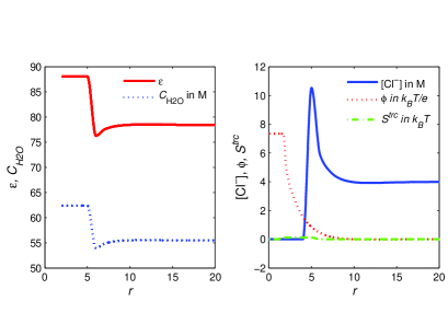
Figure 7: Dielectric function $\widetilde{\epsilon}(\mathbf{r})$ (denoted by $\varepsilon$ in the figure), water density $C_{\text{H}_{\text{2}}\text{O}}(\mathbf{r})$ ($C_{\text{H}_{\text{2}}\text{O}}$), Cl^- concentration $C_{\text{Cl}^{-}}(\mathbf{r})$ ([Cl^-]), electric potential $\phi^{\text{PF}}(\mathbf{r})$ ($\phi$), and steric potential $S^{\text{trc}}(\mathbf{r})$ ($S^{\text{trc}}$) profiles near the solvated ion Ca²⁺ at [CaCl₂] $=2$ M, where $r$ is the distance from the center of Ca²⁺ in Angstrom.

V Conclusion

A Poisson-Fermi model for calculating activity coefficients of aqueous single or mixed electrolyte solutions in a large range of concentrations and temperatures has been presented and tested by a set of experimental data. The model was shown to well fit experimental data with only three adjustable parameters at most for each activity-concentration curve. The adjustable parameters correspond to different orders of approximation of the unknown Born radius of solvation energy that depends on salt concentrations in a highly complex and nonlinear way. Nevertheless, the values of these parameters have been shown to deviate slightly in decimal digits from that of the experimental Born radius in pure water. These parameters are physically explained and can be easily verified in future studies for the same or different solutions of the present work. The model requires very few parameters because it is based on an advanced continuum theory that accounts for steric and correlation effects of ions and water with interstitial voids between nonuniform hard spheres. It also deals with short- and long-range interactions by partitioning the model domain into the ion, hydration shell, and the remaining solvent sub-domains. Numerical methods were also given to show how to solve different equations on different sub-domains that describe different physical properties of an ion in electrolyte solutions.

- (1) R. Robinson and R. Stokes, Electrolyte Solutions (Butterworths Scientific Publications, London, 1959); (Dover Publications, New York, 2002).
- (2) J. Newman, Electrochemical Systems (Prentice-Hall, NJ, 1991).
- (3) K. S. Pitzer, Thermodynamics (McGraw Hill, New York, 1995).
- (4) B. Hille, Ionic Channels of Excitable Membranes (Sinauer Associates Inc., Sunderland, MA, 2001).
- (5) K. J. Laidler, J. H. Meiser, and B. C. Sanctuary, Physical Chemistry (Houghton Mifflin Co., Boston, 2003).
- (6) W. R. Fawcett, Liquids, Solutions, and Interfaces: From Classical Macroscopic Descriptions to Modern Microscopic Details (Oxford University Press, New York, 2004).
- (7) G. Lebon, D. Jou, and J. Casas-Vázquez, Understanding Non-equilibrium Thermodynamics: Foundations, Applications, Frontiers (Springer, 2008).
- (8) G. M. Kontogeorgis and G. K. Folas, Thermodynamic Models for Industrial Applications: From Classical and Advanced Mixing Rules to Association Theories (John Wiley & Sons, 2009).
- (9) W. Kunz, Specific Ion Effects (World Scientific, Singapore 2010).
- (10) J. H. Vera and G. Wilczek-Vera, Classical Thermodynamics of Fluid Systems: Principles and Applications (CRC Press, 2016).
- (11) W. Voigt, Chemistry of salts in aqueous solutions: Applications, experiments, and theory. Pure Appl. Chem. 83, (2011) 1015-1030.
- (12) B. Eisenberg, Interacting ions in Biophysics: Real is not ideal, Biophys. J. 104, 1849-1866 (2013).
- (13) D. Rowland, E. Königsberger, G. Hefter, and P. M. May, Aqueous electrolyte solution modelling: Some limitations of the Pitzer equations, Appl. Geochem. 55, 170 (2015).
- (14) P. Debye and E. Hückel, Zur Theorie der Elektrolyte. I. Gefrierpunktserniedrigung und verwandte Erscheinunge (The theory of electrolytes. I. Lowering of freezing point and related phenomena), Phys. Zeitschr. 24, 185-206 (1923).
- (15) M. Gouy, Sur la constitution de la charge electrique a la surface d’un electrolyte (Constitution of the electric charge at the surface of an electrolyte), J. Phys. 9 (1910) 457-468.
- (16) D. L. Chapman, A contribution to the theory of electrocapillarity, Phil. Mag. 25, 475-481 (1913).
- (17) J.-L. Liu, Numerical methods for the Poisson-Fermi equation in electrolytes, J. Comput. Phys. 247, 88 (2013).
- (18) J.-L. Liu, D. Xie, and B. Eisenberg, Poisson-Fermi formulation of nonlocal electrostatics in electrolyte solutions, Mol. Based Math. Biol. 5, 116-124 (2017).
- (19) J.-L. Liu and B. Eisenberg, Poisson-Fermi model of single ion activities in aqueous solutions, Chem. Phys. Lett. 637, 1-6 (2015).
- (20) J.-L. Liu and B. Eisenberg, Correlated ions in a calcium channel model: a Poisson-Fermi theory, J. Phys. Chem. B 117, 12051 (2013).
- (21) J.-L. Liu and B. Eisenberg, Poisson-Nernst-Planck-Fermi theory for modeling biological ion channels, J. Chem. Phys. 141, 22D532 (2014).
- (22) J.-L. Liu and B. Eisenberg, Analytical models of calcium binding in a calcium channel, J. Chem. Phys. 141, 075102 (2014).
- (23) J.-L. Liu and B. Eisenberg, Numerical methods for a Poisson-Nernst-Planck-Fermi model of biological ion channels, Phys. Rev. E 92, 012711 (2015).
- (24) J.-L. Liu, H.-j. Hsieh, and B. Eisenberg, Poisson-Fermi modeling of the ion exchange mechanism of the sodium/calcium exchanger, J. Phys. Chem. B 120, 2658-2669 (2016).
- (25) M. Valiskó, D. Boda, Unraveling the behavior of the individual ionic activity coefficients on the basis of the balance of ion-ion and ion-water interactions, J. Phys. Chem. B 119, 1546 (2015).
- (26) G. Wilczek-Vera, E. Rodil, and J. H. Vera, On the activity of ions and the junction potential: Revised values for all data, AIChE. J. 50, 445 (2004).
- (27) K. S. Pitzer, J. C. Peiper, and R. H. Busey, Thermodynamic properties of aqueous sodium chloride solutions, J. Phys. Chem. Ref. Data 13, 1-102 (1984).
- (28) R. H. Busey, H. F. Holmes, and R. E. Mesmer, The enthalpy of dilution of aqueous sodium chloride to 673 K using a new heat-flow and liquid-flow microcalorimeter. Excess thermodynamic properties and their pressure coefficients, J. Chem. Thermodyn. 16, 343-372 (1984).
- (29) D. G. Archer, Thermodynamic properties of the NaCl + H2O System. II. Thermodynamic properties of NaCl(aq), NaCl.2H2O(cr), and phase equilibria, J. Phys. Chem. Ref. Data 21, 793-829 (1992).
- (30) R. N. Goldberg and R. L. Nuttall, Evaluated activity and osmotic coefficients for aqueous solutions: The alkaline earth metal halides, J. Phys. Chem. Ref. Data 7, 263-310 (1978).
- (31) P. Wang, K. S. Pitzer, and J. M. Simonson, Thermodynamic properties of aqueous magnesium chloride solutions from 250 to 600 K and to 100 MPa, J. Phys. Chem. Ref. Data 27, 971-991 (1998).
- (32) C. Christov, Chemical equilibrium model of solution behavior and bishofite (MgCl6H2O(cr)) and hydrogen-carnallite (HClMgCl7H2O(cr)) solubility in the MgCl2 + H2O and HCl-MgCl2 + H2O systems to high acid concentration at (0 to 100) , J. Chem. Eng. Data 54, 2599-2608 (2009).
- (33) R. D. Lanier, Activity coefficients of sodium chloride in aqueous three-component solutions by cation-sensitive glass electrodes, J. Phys. Chem. 69, 3992-3998 (1965).
- (34) N. Kurnakov and S. F. Zemcuzny, Equilibria in the reciprocal system sodium chloride-magnesium sulfate with particular reference to natural brines, Z. Anorg. Allg. Chem. 140, 149-182 (1924).
- (35) S. Takegami, Reciprocal salt pairs: Na2Cl2 + MgSO4 and Na2SO4 + MgCl2 at 25 , Memoirs College Sci. Kyoto Imperial Univ. 4, 317-342 (1921).
- (36) G. Wilczek-Vera and J. H. Vera, On the measurement of individual ion activities, Fluid Phase Equilibria 236, 96-110 (2005).
- (37) G. Wilczek-Vera, E. Rodil, and J. H. Vera, A complete discussion of the rationale supporting the experimental determination of individual ionic activities, Fluid Phase Equilibria 244, 33-45 (2006).
- (38) G. Wilczek-Vera and J. H. Vera, Peculiarities of the thermodynamics of electrolyte solutions: A critical discussion, Can. J. Chem. Eng. 81, 70-79 (2003).
- (39) G. Wilczek-Vera and J. H. Vera, The activity of individual ions. A conceptual discussion of the relation between the theory and the experimentally measured values, Fluid Phase Equilibria 312, 79-84 (2011).
- (40) G. Wilczek-Vera and J. H. Vera, How much do we know about the activity of individual ions? J. Chem. Thermodynamics 9, 65-69 (2016).
- (41) D. Fraenkel, Simplified electrostatic model for the thermodynamic excess potentials of binary strong electrolyte solutions with size-dissimilar ions, Mol. Phys. 108, 1435 (2010).
- (42) D. Bashford and D. A. Case, Generalized Born models of macromolecular solvation effects, Annu. Rev. Phys. Chem. 51, 129 (2000).
- (43) W. W. Rudolph and G. Irmer, Hydration of the calcium(II) ion in an aqueous solution of common anions (ClO, Cl-, Br-, and NO), Dalton Trans. 42, 3919 (2013).
- (44) J. Mähler and I. Persson, A study of the hydration of the alkali metal ions in aqueous solution, Inorg. Chem. 51, 425 (2011).
- (45) B. Eisenberg, Life’s solutions: a mathematical challenge, arXiv:1207.4737 (2012).
- (46) C. D. Santangelo, Computing counterion densities at intermediate coupling, Phys. Rev. E 73, 041512 (2006).
- (47) M. Z. Bazant, B. D. Storey, and A. A. Kornyshev, Double layer in ionic liquids: Overscreening versus crowding, Phys. Rev. Lett. 106, 046102 (2011).
- (48) I-L. Chern, J.-G. Liu, and W.-C. Wang, Accurate evaluation of electrostatics for macromolecules in solution, Methods Appl. Anal. 10, 309-328 (2003).
- (49) W. Geng, S. Yu, and G. Wei, Treatment of charge singularities in implicit solvent models, J. Chem. Phys. 127, 114106 (2007).
- (50) R. S. Dembo, S. C. Eisenstat, and T. Steihaug, Inexact Newton methods, SIAM J. Numer. Anal. 19, 400-408 (1982).
- (51) D. P. Fernandez, A. R. H. Goodwin, E. W. Lemmon, J. L. Sengers, and R. C. Williams, A formulation for the static permittivity of water and steam at temperatures from 238 K to 873 K at pressures up to 1200 MPa, including derivatives and Debye–Hückel coefficients, J. Phys. Chem. Ref. Data 26, 1125-1166 (1997).
- (52) S. Mao and Z. Duan, The properties of binary aqueous chloride solutions up to T = 573 K and 100 MPa, J. Chem. Thermodynamics 40, 1046-1063 (2008).