A search for Cyanopolyynes in L1157-B1

Abstract

We present here a systematic search for cyanopolyynes in the shock region L1157-B1 and its associated protostar L1157-mm in the framework of the Large Program "Astrochemical Surveys At IRAM" (ASAI), dedicated to chemical surveys of solar-type star forming regions with the IRAM 30m telescope. Observations of the millimeter windows between 72 and 272 GHz permitted the detection of HC₃N and its 13C isotopologues, and HC₅N (for the first time in a protostellar shock region). In the shock, analysis of the line profiles shows that the emission arises from the outflow cavities associated with L1157-B1 and L1157-B2. Molecular abundances and excitation conditions were obtained from analysis of the Spectral Line Energy Distributions under the assumption of Local Thermodynamical Equilibrium or using a radiative transfer code in the Large Velocity Gradient approximation. Towards L1157mm, the HC₃N emission arises from the cold envelope ($T_{rot}=10\hbox{\kern 1.99997ptK}$) and a higher-excitation region ($T_{rot}$= $31\hbox{\kern 1.99997ptK}$) of smaller extent around the protostar. We did not find any evidence of ¹³C or D fractionation enrichment towards L1157-B1. We obtain a relative abundance ratio HC₃N/HC₅N of 3.3 in the shocked gas. We find an increase by a factor of 30 of the HC₃N abundance between the envelope of L1157-mm and the shock region itself. Altogether, these results are consistent with a scenario in which the bulk of HC₃N was produced by means of gas phase reactions in the passage of the shock. This scenario is supported by the predictions of a parametric shock code coupled with the chemical model UCL_CHEM.

1 Introduction

Cyanopolyynes (HC_2n+1N) are molecules found in a wide range of environments in our Galaxy, from comets in our Solar System (Crovisier et al. 2004) to molecular clouds (Takano et al 1998, 2014) and evolved stars (Cernicharo & Guélin 1996). In star-forming regions, only relatively short chains have been reported in the literature so far, up to HC₁₁N, in dense cold cores (Bell et al. 1997) and hydrocarbon-rich protostellar envelopes of low-mass (WCCC) sources (e.g. Sakai et al. 2008; Cordiner et al. 2012; Friesen et al. 2013).

An important property of cyanopolyynes is their stability against strong radiation field and cosmic rays (Clarke & Ferris 1995). Recently, Jaber Al-Edhari et al. (2017) showed how the cyanopolyyne emission properties could be used to trace the history of the IRAS16293-2422 protostellar envelope.

The presence of cyanopolyynes in protostellar shock regions has received relatively little attention, since the detection of HC₃N by Bachiller & Perez-Gutíerrez (1997) in the outflow shocks of L1157, a low-mass star forming region at $\sim$250 pc (Looney et al. 2007). They estimated an increase of the molecular abundance by about 2 orders of magnitude between the outflow shock regions L1157-B1/B2 and the position of the protostar L1157-mm. Their estimate was based on a simple LTE analysis of 3 transitions, only. No evidence for more complex cyanopolyyne (HC₅N) was found. The survey of L1157-B1 in the 3mm window with the 45m telescope of the Nobeyama Radio Observatory by Yamaguchi et al. (2012) only confirmed the above results, and no substantial advances were made in the chemistry of cyanopolyynes and the presence of longer chains.

The outflow shock region L1157-B1 and the outflow driving protostar L1157-mm have been the subject of a thorough study by our team, in particular as part of the observational Large Program “Astrochemical Surveys At IRAM”(̈ASAI; Lefloch et al. 2017 in prep.) with the IRAM 30m telescope. These various studies have provided us with a unique dataset, which offers the possibility of investigating the physical and chemical structure of a typical protostellar shock (Lefloch et al. 2010, 2012, 2016, 2017; Benedettini et al. 2012, 2013; Codella et al. 2010, 2012, 2015, 2017; Busquet et al. 2014; Podio et al. 2014, 2016, 2017).

In this work, we present an observational study on the chemistry of cyanopolyynes, in a shock region, as well as the impact of protostellar shock on the chemical conditions in the ambient cloud. The paper is organized as follows. In Sect. 2, we summarize the main observational properties of the shock region L1157-B1. The observations are described in Sect. 3. In Sect. 4, we present the molecular transitions of cyanpolyynes detected in the ASAI line survey. The properties of the shock, the origin of the emission and the shock physical conditions (density, temperature, abundance) are discussed in Section 5. The cyanopolyyne emission towards the protostar is presented in Section 6. We discuss our results in Section 7. Finally, we present our conclusions in Section 8.

2 The L1157-B1 shock region

Table 1: Outflow shock components and their physical conditions in the L1157-B1 shock region, from CO and CS emission. The H₂ column densities were obtained from the CO column densities derived by Lefloch et al. (2012), adopting a CO/H₂ abundance ratio of $10^{-4}$ (see also Gómez-Ruiz et al. 2015).

	Vel. range	$v_{0}$	T	n(H2)	N(H2)	Size	Origin
	(kms-1)	(kms-1)	(K)	(cm-3)	(cm-2)	($\arcsec$)
$g_{1}$	-40; 0	12	210	$\geq 1.0(6)$	0.9(20)	7–10	jet impact region
$g_{2}$	-20; 0	4	64	$\sim$ 1.0(6)	0.9(21)	20	B1 outflow cavity walls
$g_{3}$	-8; 0	2	23	(0.5–2)(5)	1.0(21)	Extended	B2 outflow cavity walls

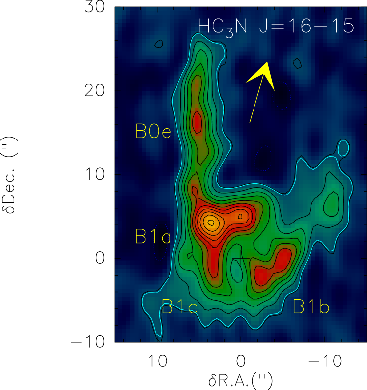
Figure 1: The L1157-B1 bow-shock region as traced by the HC₃N(16–15) emission, observed with the PdB interferometer (from Benedettini et al. 2013). The location of the individual shocked clumps B1a-b-c and B0e indicated (Benedettini et al. 2013). The arrow points to the direction of the L1157-mm protostar. The first contour and steps correspond to 5$\sigma$ (170 mJy beam^-1 km s^-1) and 3$\sigma$, respectively.

The L1157 bipolar and chemically rich molecular outflow (Bachiller et al. 2001) is swept up by an episodic and precessing jet (Gueth et al. 1996, 1998; Tafalla et al. 2015; Podio et al. 2016) driven by the L1157-mm Class 0 protostar. The blue-shifted southern lobe mainly consists of two main cavities with different kinematical ages: B1 ($\approx$ 1100 yr), and the older and more extended B2 (1800 yr). The bright bow shock at the B1 cavity is located at $\sim$ 69$\arcsec$ (0.1 pc) from the protostar (see Fig. 1), and various molecular tracers indicate warm shocked gas enriched by the injection of dust mantle and core products, such as CH₃OH, NH₃, H₂CO, NH₂CHO (see e.g. Tafalla & Bachiller 1995; Benedettini et al. 2012; Codella et al. 2010, 2017; Mendoza et al. 2014; Lefloch et al. 2017; and references therein). High-angular resolution observations of these tracers with the Plateau de Bure Interferometer (PdBI) reveal the presence of a few high-velocity clumps (B1a-b-c and B0e) whereas the lower velocity material traces the expansion of the cavity excavated by the shock (see e.g. Benedettini et al. 2013).

Previous analysis of the CO and CS gas kinematics, as observed with the IRAM 30m telescope (Lefloch et al. 2012; Gómez-Ruiz et al. 2015), has led to identify three physically distinct components coexisting in L1157-B1, labelled as follows and summarized in Table 1:

• $g_{1}$: the region of $\sim$7$\arcsec$–10$\arcsec$ at $T_{\rm kin}$ $\sim$ 210 K and $n_{\rm H_{2}}$ $\geq$ 10⁶ cm${-3}$, associated with a dissociative J-shock due to the youngest impact of the jet against the B1 cavity walls.

• $g_{2}$: the outflow cavity walls ($\sim$ 20$\arcsec$, 60–80 K, 10⁵–10⁶ cm^-3) associated with the B1 ejection.

• $g_{3}$: the older outflow cavity walls (extended, 20 K, $\simeq$ 10⁵ cm^-3) associated with the B2 ejection.

Lefloch et al. (2012) and Gómez-Ruiz et al. (2015) showed that each component is characterized by homogeneous excitation conditions independent of the velocity range (see Table 1). The intensity-velocity distribution of each component is well described by an exponential law $T_{b}(v)\propto exp(v/v_{0})$, where $v_{0}$ is almost independent of the molecular transition considered ($v_{\rm 0}$ = 12.5, 4.4, and 2.5 km s^-1 for $g_{1}$, $g_{2}$, and $g_{3}$, respectively).

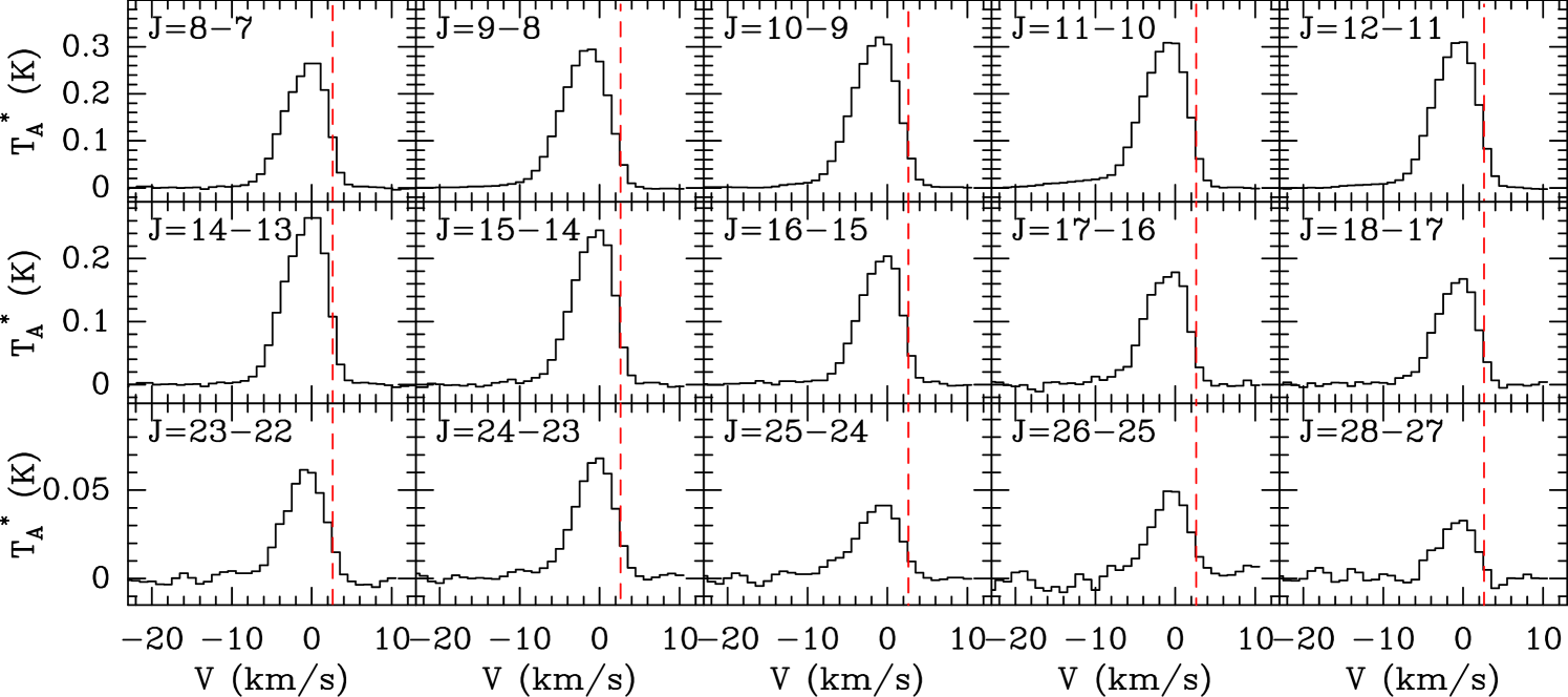
Figure 2: Montage of some HC₃N lines detected towards L1157-B1. The red line (dashed) draws the velocity of the cloud ($v_{lsr}=+2.6\hbox{\kern 1.99997ptkm\kern 1.99997pts${}^{-1}$}$).

3 Observations

Observations of the IRAM Large Program ASAI were carried out during several runs between September 2012 and March 2015. The nominal position observed are $\alpha_{J2000}=$ 20${}^{\text{h}}$ 39${}^{\text{m}}$ 10.${}^{\text{s}}$2, $\delta_{J2000}=$ +68^∘ 01^′ 10^′′ and $\alpha_{J2000}=$ 20${}^{\text{h}}$ 39${}^{\text{m}}$ 06.${}^{\text{s}}$3, $\delta_{J2000}=$ +68^∘ 02^′ 15.8^′′ for L1157-B1 and L1157-mm, respectively.

Data were collected using the broad-band EMIR (Eight MIxer Receiver) receivers at 3 mm, 2 mm, 1.3 mm, whose interval frequencies are 72 – 116 GHz, 128 –173 GHz, 200 – 272 GHz, respectively. Both the Fast Fourier Transform Spectrometers and the WILMA backends were connected to the EMIR receivers providing a spectral resolution of $\sim$ 200 kHz and 2 MHz, respectively. The FTS spectral resolution was degraded to a final velocity resolution of $\approx 1\hbox{\kern 1.99997ptkm\kern 1.99997pts${}^{-1}$}$. In order to ensure a flat baseline across the spectral bandwith observed, the observations were carried out in Wobbler Switching Mode, with a throw of $3^{\prime}$.

For the ASAI data, the reduction was performed using the GILDAS/CLASS software. The calibration uncertainties are typically 10, 15, and 20% at 3 mm, 2 mm and 1.3 mm, respectively. The line intensities are expressed in units of antenna temperature corrected for atmospheric attenuation and rearward losses ($T_{A}^{\ast}$). For subsequent analysis, fluxes are expressed in main beam temperature units ($T_{mb}$). The telescope and receiver parameters (beam efficiency, Beff; forward efficiency, Feff; Half Power beam Width, HPBW) were taken from the IRAM webpage.

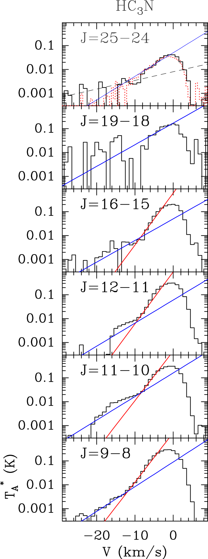
Figure 3: Montage of some HC₃N spectra detected towards L1157-B1. We have superimposed the fit obtained by a linear combination of two exponential functions $g_{2}\propto\exp(-v/4.0)$ (blue) and $g_{3}\propto\exp(-v/2.0)$ (red). In the top panel ($J=25-24$), a fit of the $g_{1}$ component ($\propto\exp(-v/12)$) is superimposed in black and the CS $J$=7–6 line (a proxy for the $g_{2}$ component) is superimposed in dotted red.

4 Cyanopolyyne emission in L1157-B1

The ASAI survey permitted the identification of several rotational transitions of HC₃N and HC₅N. The sensitivity of the survey permitted the detection of a few transitions of the ¹³C isotopologues of HC₃N. We failed to detect larger cyanopolyynes as a search for HC₇N yielded only negative results. In this section, we describe the spectral signatures of HC₃N and HC₅N.

4.1 HC₃N

We detected all the HC₃N rotational transitions falling in the ASAI bands, from $J$=8–7 ($E_{up}$= $16\hbox{\kern 1.99997ptK}$) up to $J$=29–28 ($E_{up}$= $189.9\hbox{\kern 1.99997ptK}$). The spectra are displayed in Fig. 2. The line spectroscopic and observational properties are summarized in Table 2.

The bulk of the emission peaks at $-1\hbox{\kern 1.99997ptkm\kern 1.99997pts${}^{-1}$}$, with a linewidth (FWHM) ranging between 5 and $6\hbox{\kern 1.99997ptkm\kern 1.99997pts${}^{-1}$}$ (see Table 2). In the transitions with $J_{up}\leq 16$, emission is detected up to $v_{lsr}$= $-20\hbox{\kern 1.99997ptkm\kern 1.99997pts${}^{-1}$}$. The intensity-velocity distribution can be well fit adopting a relation of the type $T\propto exp(v/v_{0})$ with $v_{0}$= $+4\hbox{\kern 1.99997ptkm\kern 1.99997pts${}^{-1}$}$, independently of the rotational number of the transition (Fig. 3). This spectral signature has been observed in all the transitions, up to $J$=25–24. In the lower $J$ transitions, from $J$=8–7 to $J$=19–18, a second emission component with a lower velocity range, between 0 and $-8\hbox{\kern 1.99997ptkm\kern 1.99997pts${}^{-1}$}$, is detected. It can be fit by a second exponential component with an exponent $v_{0}$= $+2\hbox{\kern 1.99997ptkm\kern 1.99997pts${}^{-1}$}$, which, again, does not vary with $J_{up}$ (Fig. 3).

This confirms that at least the high-$J$ HC₃N line emission arises from component $g_{2}$, i.e. the outflow cavity associated with L1157-B1. In the top right panel of Fig. 3, we have superimposed the CS $J$=7–6 spectrum (dashed red) on the HC₃N $J$=25–24 line profile, applying a scaling factor so to match the peak intensity. We find an excellent match between both line profiles over the full emission range. This indicates that the high-$J$ ($J\geq 25$) HC₃N line emission arises from component $g_{2}$. This point is further addressed in Sect. 5.

This profile decomposition is justified by the fact that the HC₃N line emission is optically thin, except at velocities close to that of the ambient cloud for the low-$J$ transitions. We note however that the frequency of the transitions $J_{up}$= 8–12 is low enough that the telescope beam encompasses the shock region B0 (Fig. 1), which is associated with another ejection (Bachiller et al. 2001), so that the emission collected, and the line profiles, could be contaminated by this shock region. This point is addressed further below in Sect. 5.3.

Table 2: L1157-B1. Spectroscopic and observational parameters of the lines from HC₃N, its isotopologues, and HC₅N identified towards the protostellar shock L1157-B1. We give in bracket the statistical uncertainties on the observational parameters, as derived from a gauss fit to the profiles.

Transition	Frequency	$E_{u}$	$A_{ul}$	HPBW	$\eta_{mb}$	$\int T_{mb}dv$	FWHM	$V_{lsr}$
$J\rightarrow J-1$	MHz	K	s-1	′′		mK km s-1	km s-1	km s-1
HC3N
8 – 7	72783.822	15.7	2.94(-5)	33.8	0.86	2044(3)	5.9(0.1)	-0.7(0.1)
9 – 8	81881.468	19.7	4.21(-5)	30.0	0.85	2556(4)	6.2(0.2)	-1.7(0.1)
10 – 9	90979.023	24.0	5.81(-5)	27.0	0.84	2674(4)	6.1(0.2)	-1.4(0.1)
11 – 10	100076.392	28.8	7.77(-5)	24.6	0.84	2729(7)	6.2(0.1)	-1.3(0.1)
12 – 11	109173.634	34.1	1.01(-4)	22.5	0.83	2560(7)	5.9(0.1)	-1.0(0.1)
14 – 13	127367.666	45.9	1.62(-4)	19.3	0.81	1790(8)	5.8(0.1)	-0.9(0.1)
15 – 14	136464.411	52.4	1.99(-4)	18.0	0.81	1951(9)	5.8(0.1)	-0.8(0.1)
16 – 15	145560.960	59.4	2.42(-4)	16.9	0.79	1659(9)	5.8(0.1)	-0.9(0.1)
17 – 16	154657.284	66.8	2.91(-4)	15.9	0.77	1516(19)	5.9(0.1)	-1.1(0.1)
18 – 17	163753.389	74.7	3.46(-4)	15.0	0.77	1370(12)	5.6(0.1)	-0.8(0.1)
19 – 18	172849.301	83.0	4.08(-4)	14.2	0.75	1248(92)	5.9(0.3)	-1.1(0.2)
23 – 22	209230.234	120.5	7.26(-4)	11.8	0.67	543(9)	5.7(0.2)	-0.8(0.1)
24 – 23	218324.723	131.0	8.26(-4)	11.3	0.65	611(10)	5.3(0.2)	-0.6(0.1)
25 – 24	227418.905	141.9	9.35(-4)	10.8	0.64	430(8)	6.1(0.3)	-1.1(0.1)
26 – 25	236512.789	153.2	1.05(-3)	10.4	0.63	451(14)	5.3(0.4)	-0.6(0.1)
27 – 26	245606.320	165.0	1.18(-3)	10.0	0.62	273(10)	7.1(0.4)	-0.9(0.2)
28 – 27	254699.500	177.3	1.32(-3)	9.7	0.60	289(12)	4.9(0.4)	-0.8(0.2)
29 – 28	263792.308	189.9	1.46(-3)	9.3	0.60	187(16)	5.0(0.8)	-0.5(0.3)
H13CCCN
10 – 9	88166.832	23.3	5.29(-5)	27.9	0.85	40.7(4.5)	7.1(1.4)	-1.8(0.5)
11 – 10	96983.001	27.9	7.07(-5)	25.4	0.85	76.0(4.8)	7.2(1.0)	-0.8(0.4)
12 – 11	105799.113	33.0	9.21(-5)	23.3	0.84	48.1(3.9)	5.2(0.8)	-2.3(0.3)
HC13CCN
9 – 8	81534.111	19.6	4.16(-5)	30.2	0.86	55.8(2.7)	6.1(0.9)	-2.7(0.3)
10 – 9	90593.059	23.9	5.74(-5)	27.2	0.85	43.1(3.7)	6.5(1.5)	-3.8(0.5)
11 – 10	99651.849	28.7	7.67(-5)	24.7	0.84	43.6(5.2)	5.0(1.7)	-0.4(0.7)
12 – 11	108710.532	33.9	1.00(-4)	22.6	0.83	31.3(5.0)	6.1(2.7)	-0.7(0.9)
HCC13CN
9 – 8	81541.981	19.6	4.16(-5)	30.2	0.86	25.7(3.1)	4.5(1.4)	-0.7(0.6)
10 – 9	90601.777	23.9	5.74(-5)	27.2	0.85	38.1(4.2)	4.8(1.6)	-1.8(0.6)
11 – 10	99661.467	28.7	7.67(-5)	24.7	0.84	33.3(5.3)	4.5(2.0)	-1.1(0.8)
12 – 11	108720.999	33.9	1.00(-4)	22.6	0.83	35.5(3.4)	4.0(0.7)	-0.4(0.3)
HC5N
30 – 29	79876.710	59.4	5.47(-5)	30.8	0.86	39.1(3.4)	3.5(0.8)	-1.5(0.3)
31 – 30	82539.039	63.4	6.04(-5)	29.8	0.85	22.5(1.7)	3.7(0.8)	-1.7(0.3)
32 – 31	85201.346	67.5	6.64(-5)	28.9	0.85	34.1(1.7)	5.0(0.8)	-1.9(0.3)
33 – 32	87863.630	71.7	7.29(-5)	28.0	0.85	47.1(1.5)	7.4(1.0)	-1.8(0.4)
34 – 33	90525.889	76.0	7.98(-5)	27.2	0.85	37.1(1.7)	6.3(1.2)	-1.5(0.5)
35 – 34	93188.123	80.5	8.71(-5)	26.4	0.85	30.8(2.6)	5.4(2.3)	-0.6(0.7)
36 – 35	95850.335	85.1	9.48(-5)	25.7	0.85	36.0(2.4)	5.7(1.4)	-0.4(0.6)
37 – 36	98512.524	89.8	1.03(-4)	25.0	0.84	27.9(1.2)	3.5(0.8)	1.8(0.6)
38 – 37	101174.677	94.7	1.12(-4)	24.3	0.84	38.2(2.0)	7.6(2.1)	-2.2(0.9)
39 – 38	103836.817	99.7	1.21(-4)	23.7	0.84	31.1(2.0)	6.0(1.6)	-2.7(0.6)
40 – 39	106498.910	104.8	1.30(-4)	23.1	0.84	39.2(2.2)	5.0(1.0)	0.2(0.4)
41 – 40	109160.973	110.0	1.40(-4)	22.5	0.83	28.2(2.2)	5.0(2.1)	-2.3(0.8)
42 – 41	111823.024	115.4	1.51(-4)	22.0	0.83	45.0(3.4)	4.4(1.0)	0.2(0.4)
43 – 42	114485.033	120.9	1.62(-4)	21.5	0.83	23.0(3.9)	2.9(1.1)	-0.8(0.5)

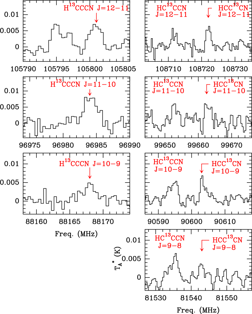
Figure 4: Montage of the detected transitions from the rare isotopologues H¹³CCCN, HC¹³CCN and HCC¹³CN.

The search for the HC₃N isotopologues yielded positive results in the band at 3 mm. We detected the transitions H¹³CCCN $J$=10–9, 11–10 and 12–11; HC¹³CCN $J$=9–8, 10–9, 11–10, 12–11; and HCC¹³CN $J$=9–8, 10–9, 11–10 and 12–11, whose line profiles are displayed in Fig. 4. Intensity of all the transitions is weak, typically 5 mK ($T_{A}^{*}$), so that the line parameters determination suffers large uncertainties. Their properties are summarized in Table 2.

We searched for emission lines from the deuterated isotopologue of HC₃N, following the previous work by Codella et al. (2012) on the fossile deuteration in L1157-B1. We failed to detect any of the transitions falling in the 3mm ASAI band, down to a $3\sigma$ level of 4 mK ($T_{A}^{*}$).

4.2 HC₅N

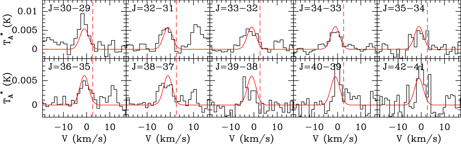
Figure 5: Montage of some HC₅N transitions detected towards L1157-B1. The best fit obtained from a simple rotational diagram analysis is shown in red, adopting a linewidth $\Delta v$= $5\hbox{\kern 1.99997ptkm\kern 1.99997pts${}^{-1}$}$. The ambient cloud velocity ($v_{lsr}$= $+2.6\hbox{\kern 1.99997ptkm\kern 1.99997pts${}^{-1}$}$) is marked by the dash-dotted line.

Only transitions in the 3mm band, between 80 and 114 GHz, could be detected. All the transitions from $J$=30–29 ($E_{up}$= $59\hbox{\kern 1.99997ptK}$) to $J$=43–42 ($E_{up}$= $121\hbox{\kern 1.99997ptK}$) were detected down to the $3\sigma$ level (Table 2). Line intensities are rather weak, typically 5–10mK, a factor $\sim 20$ less than HC₃N transitions of similar $E_{up}$. We show a montage of some HC₅N lines detected towards L1157-B1 in Fig. 5. The typical line width (FWHM) and the emission peak velocity are $\simeq 4.5\hbox{\kern 1.99997ptkm\kern 1.99997pts${}^{-1}$}$ and $-1\hbox{\kern 1.99997ptkm\kern 1.99997pts${}^{-1}$}$, respectively, hence in good agreement with the parameters of the HC₃N lines. The analysis of the excitation conditions (see Sect. 5.3 below) leads us to conclude that the emission of HC₅N is dominated by $g_{2}$.

5 Physical conditions and abundances in L1157-B1

The physical conditions and the column densities of HC₃N and HC₅N were obtained from the analysis of their Spectral Line Energy Distribution (SLED) via a Large-Velocity Gradient (LVG) modelling and under the assumption of Local Thermodynamic Equilibrium (LTE), respectively. We discuss the two cases separately.

5.1 HC₃N

As discussed in the previous section, the HC₃N line emission can be decomposed in two components, $g_{2}$ and $g_{3}$, which probe the outflow cavity walls of B1 and B2, respectively. Figure 6 shows the Spectral Line Energy Distribution (SLED) of the two components. While the $g_{3}$ SLED peaks at J$\sim$11, the $g_{2}$ SLED clearly shows two different peaks, at J$\leq$8 and J$\sim$20, suggesting the presence of a cold and a warm physical component.

Before modelling the SLED of each component, we first estimated the brightness temperature of the molecular lines. Our previous studies of CO and CS showed that the component $g_{3}$ is extended enough that the brightness temperature of the lines can be approximated by the main-beam brightness temperature $T_{mb}$.

As the source size of component $g_{2}$ is not precisely known, we have chosen to perform the SLED modeling at a common angular resolution of $8.5\arcsec$ (the HPBW at the frequency of the J=32-31 line, the highest detected transition of HC₃N in L1157-B1), for all the transitions. It means that the effective column density derived for the $g_{2}$ component scales as the effective filling factor in the $8.5\arcsec$ beam. To do so, we followed the methodology presented in Lefloch et al. (2012) and Gomez-Ruiz et al. (2015). The $g_{2}$ and $g_{3}$ velocity integrated fluxes used in our SLED analysis are reported in Table 3.

Taking into account the uncertainties in the spectral decomposition of component $g_{2}$ and $g_{3}$, we estimate the total uncertainties to be 15%, 20%, 25% at 3mm, 2mm and 1.3mm, respectively.

To model the SLED emission, we used the LVG code by Ceccarelli et al. (2002) and used the collisional coefficients with para and ortho H₂ computed by Faure et al. (2016). For the H₂ ortho-to-para ratio we assumed the fixed value of 0.5, as suggested by previous observations. We ran a large grid of models with density between $10^{4}\hbox{\kern 1.99997ptcm${}^{-3}$}$ and $10^{8}\hbox{\kern 1.99997ptcm${}^{-3}$}$, temperature between $15\hbox{\kern 1.99997ptK}$ and $120\hbox{\kern 1.99997ptK}$ and the HC₃N column density between $2\times 10^{12}$ and $3\times 10^{14}\hbox{\kern 1.99997ptcm${}^{-2}$}$. We adopted $\Delta V$= $5.5\hbox{\kern 1.99997ptkm\kern 1.99997pts${}^{-1}$}$ and let the filling factor to be a free parameter in the case of the $g_{2}$ component. We then compared the LVG predictions and the observations and used the standard minimum reduced $\chi^{2}$ criterium to constrain the four parameters: density, temperature, column density and size (in $g_{2}$ only).

Table 3: HC₃N velocity-integrated intensities of the components $g_{2}$ and $g_{3}$ used in the radiative transfer calculations. Fluxes are expressed in units of brightness temperature in a beam of $8.5\arcsec$ for $g_{2}$ and in main-beam brightness temperature for $g_{3}$, respectively.

Transition	Frequency	ff ($g_{2}$)	Flux ($g_{2}$)	Flux ($g_{3}$)
	(MHz)		K kms-1	K kms-1
8 – 7	72783.822	0.184	3.34	1.43
9 – 8	81881.468	0.227	3.23	1.83
10 – 9	90979.023	0.268	2.91	1.89
11 – 10	100076.392	0.310	2.52	1.95
12 – 11	109173.634	0.354	2.24	1.77
14 – 13	127367.666	0.437	1.02	1.34
15 – 14	136464.411	0.482	0.97	1.49
16 – 15	145560.960	0.522	1.13	1.07
17 – 16	154657.284	0.563	1.29	0.91
18 – 17	163753.389	0.603	1.01	0.76
19 – 18	172849.301	0.642	0.90	0.40
23 – 22	209230.234	0.775	0.70	0.0
24 – 23	218324.723	0.807	0.76	0.0
25 – 24	227418.905	0.839	0.51	0.0
26 – 25	236512.789	0.866	0.52	0.0
27 – 26	245606.320	0.892	0.30	0.0
28 – 27	254699.500	0.914	0.32	0.0
29 – 28	263792.308	0.942	0.20	0.0

The best fitting LVG solutions are shown in Fig. 6.

The $g_{3}$ component SLED is well reproduced by an HC₃N column density $N$(HC₃N)= $2.5\times 10^{13}\hbox{\kern 1.99997ptcm${}^{-2}$}$, a temperature of 20 K and a density $n(\hbox{H${}_{2}$})$ $\simeq 2\times 10^{6}\hbox{\kern 1.99997ptcm${}^{-3}$}$. Adopting an H₂ column density of $10^{21}\hbox{\kern 1.99997ptcm${}^{-2}$}$ for $g_{3}$ (Table 1; Lefloch et al. 2012), we find a relative abundance X(HC₃N)= $2.5\times 10^{-8}$.

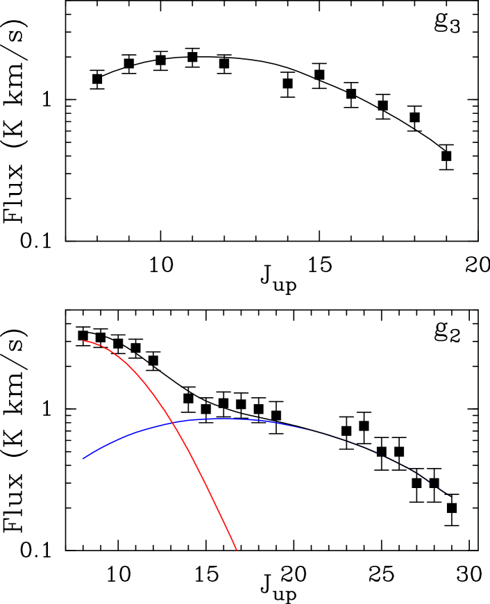
Figure 6: Modelling of the HC₃N Spectral Line Energy Distribution (SLED) with a simple LVG slab model. The black squares represent the measured velocity-integrated fluxes for components $g_{2}$ (bottom) and $g_{3}$ (top). They are expressed in units of main-beam brightness temperatures ($T_{mb}$). (Top panel:) The solid curve shows the LVG predictions for component $g_{3}$ assuming one single gas component with a column density $N$(HC₃N)=2.5$\times 10^{13}\hbox{\kern 1.99997ptcm${}^{-2}$}$, a temperature of 20 K and a density $n(\hbox{H${}_{2}$})$ $2\times 10^{6}\hbox{\kern 1.99997ptcm${}^{-3}$}$. (Bottom panel:) The solid curves show the LVG predictions for component $g_{2}$, obtained assuming two components at $20\hbox{\kern 1.99997ptK}$ (red), with density n(H₂)= $6\times 10^{4}\hbox{\kern 1.99997ptcm${}^{-3}$}$, N(HC₃N)= $2\times 10^{13}\hbox{\kern 1.99997ptcm${}^{-2}$}$ and at $60\hbox{\kern 1.99997ptK}$ (blue), with density n(H₂)= $4\times 10^{6}\hbox{\kern 1.99997ptcm${}^{-3}$}$, N(HC₃N)= $4\times 10^{12}\hbox{\kern 1.99997ptcm${}^{-2}$}$, respectively.

For the $g_{2}$ component, our modelling of the high-excitation lines ($J_{up}$=14–29) shows that the best fit is obtained for N(HC₃N)=$4\times 10^{12}\hbox{\kern 1.99997ptcm${}^{-2}$}$, $T_{kin}$= $60\hbox{\kern 1.99997ptK}$ and $n(\hbox{H${}_{2}$})$=$4\times 10^{6}\hbox{\kern 1.99997ptcm${}^{-3}$}$, and a filling factor of 0.82, corresponding to a source size of $18\arcsec$. This simple model fails however to reproduce the low excitation range $J_{up}$=8–12 of the SLED (see Fig. 6). A second gas component with a lower density $n(\hbox{H${}_{2}$})$= $6\times 10^{4}\hbox{\kern 1.99997ptcm${}^{-3}$}$ and lower temperature T=$20\hbox{\kern 1.99997ptK}$, is needed to account for the total observed flux. We estimate for this component a column density N(HC₃N)=$2\times 10^{13}\hbox{\kern 1.99997ptcm${}^{-2}$}$, and a size of $10\arcsec$. These physical conditions differ from those of $g_{2}$ and $g_{3}$ (see also Sect. 2). As pointed out in Sect. 4.1, in the frequency range corresponding to the $J$=8–12 transitions, the beam size is large enough ($\geq 23\arcsec$) that it encompasses the shock region B0, which thereby contributes to the collected emission. Conversely, at frequencies higher than that of the $J$=15–14 line, the beam size (HPBW) is about $\leq 18\arcsec$, and the telescope beam misses the B0 emission. This is probably the cause of the observed excess in the low J emission lines. We note that the density of the high-velocity bullets reported by Benedettini et al. (2013) is lower by a factor of a few in the B0 region, as compared to the B1 region; it is in agreement with the values obtained in the present analysis. Also, Lefloch et al. (2012) showed that the $g_{2}$ spectral signature was actually detected along the entire walls of the B1 cavity, between the protostar L1157-mm and the apex where bright molecular emission is detected. Proceeding as above for component $g_{3}$, we obtain an abundance of $4\times 10^{-9}\hbox{\kern 1.99997ptcm${}^{-2}$}$ for HC₃N in component $g_{2}$.

To summarize, the HC₃N emission arises from two physical components, $g_{3}$ and $g_{2}$ respectively, with an abundance relative to H₂ of $2.5\times 10^{-8}$ and $4\times 10^{-9}$, respectively. These results are consistent with the previous work by Bachiller & Pérez-Gutíerrez (1997). These authors estimated an abundance relative to H₂ of $1.0\times 10^{-8}$, assuming one single gas component, from the detection of the three HC₃N $J$=10–9, 15–14, 14–23 lines in the shock. Interestingly, the abundance of HC₃N towards $g_{2}$ appears lower than towards $g_{3}$, as low as a factor of 6.

5.2 The rare isotopologues of HC₃N

5.2.1 H¹³CCCN, HC¹³CCN, and HCC¹³CN

Only the transitions from H¹³CCCN, HC¹³CCN, and HCC¹³CN with $E_{up}$ between 19 and $34\hbox{\kern 1.99997ptK}$ were detected. The low number (3–4) of detected transitions for each isotopologue prevents us from carrying out a detailed analysis of the emission, similar to the approach adopted for HC₃N. In addition, our analysis of the HC₃N emission shows that in this range of $E_{up}$, the emission is dominated by $g_{3}$ and most probably contaminated by emission from the shock region B0, so that even a rotational diagram analysis would be somewhat not significant.

We have just simply assumed that the emission of the ¹³C-bearing isotopes and of the main isotope in the J=9–8 to J=12–11 lines originate from the same gas so that the corresponding line fluxes ratios provide a reliable measurement of the molecular abundance ratios if the main isotopologue is optically thin. The mean flux ratios are $52\pm 15$, $63\pm 20$, $81\pm 10$, for HC¹³CCN, HC¹³CCN and HCC¹³CN, respectively. These results do not show any significant difference between the three ¹³C-bearing isotopes that could indicate a differential ¹³C fractionation between the three HC₃N isotopologues. These molecular abundance ratios are also consistent with a standard value for the elemental abundance ratio ¹²C/¹³C of 70, which is consistent with the ¹²C isotopologue being optically thin.

5.2.2 DC₃N

None of the DC₃N lines falling in the 3mm band were detected, down to an rms of 1.4 mK. We obtained an upper limit on the column density of DC₃N in the LTE approximation. We adopted the value $T_{rot}$= $25\hbox{\kern 1.99997ptK}$, obtained for HC₃N in the same range of $E_{up}$ (18–$69\hbox{\kern 1.99997ptK}$). Since the HC₃N emission is dominated by component $g_{3}$ in this range of $E_{up}$, we assumed DC₃N to arise from the same region, and to be extended. We obtain as upper limit N(DC₃N)= $5\times 10^{10}\hbox{\kern 1.99997ptcm${}^{-2}$}$, from which we derive an upper limit on the abundance [DC₃N]= $5\times 10^{-11}$ and the deuterium fractionation ratio D/H= 0.002.

5.3 HC₅N

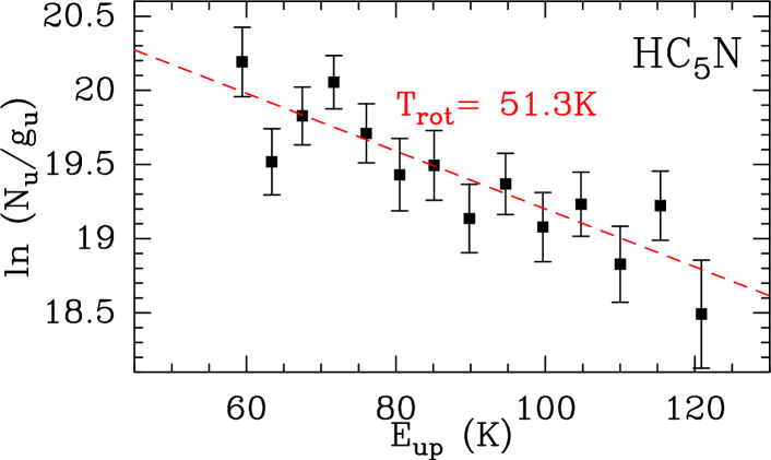
Figure 7: Rotational diagram of HC₅N. The emission was corrected for the coupling between the source and the telescope beam assuming a typical size of $18\arcsec$.

The physical conditions of HC₅N were obtained from a simple rotational diagram analysis, as shown in Fig. 7. The spatial distribution of HC₅N is not constrained and we considered two cases: a) HC₅N arises from $g_{3}$, and the emission is so extended that the line brightness is well approximated by the line main-beam temperature; b) HC₅N arises from $g_{2}$, with a typical size of $18\arcsec$. Case a) can be ruled out as the best fitting solution provides a rotational temperature $T_{rot}=87\pm 26\hbox{\kern 1.99997ptK}$, which is not consistent with the kinetic temperature of that component (20–$25\hbox{\kern 1.99997ptK}$). For case b), the emission of the detected transitions can be reasonably well described by one gas component with $T_{rot}$= $(51.3\pm 8.9)\hbox{\kern 1.99997ptK}$ and column density N(HC₅N)= $(1.2\pm 0.4)\times 10^{12}\hbox{\kern 1.99997ptcm${}^{-2}$}$. This is consistent with the gas kinetic temperature of component $g_{2}$ ($\approx 60\hbox{\kern 1.99997ptK}$). Based on our analysis of the excitation conditions we conclude that the emission of HC₅N is dominated by $g_{2}$ and the abundance [HC₅N] is $\approx 1.2\times 10^{-9}$. The best fitting solution to the line profiles is shown in Fig. 5. We note that the HC₃N column density is $\simeq 4.0\times 10^{12}\hbox{\kern 1.99997ptcm${}^{-2}$}$ in the same range of excitation conditions, hence the relative abundance ratio HC₃N/HC₅N $\simeq 3.3$.

5.4 HC₇N

The non-detection of HC₇N could be due to a lower abundance (like in TMC1) and/or to less favourable excitation conditions than for the smaller cyanopolyynes. The lowest frequency transition in the ASAI band is $J$=64–63 72187.9088 MHz has an $E_{up}$= $112.6\hbox{\kern 1.99997ptK}$. Between 80 and 114 GHz, the frequency interval in which HC₅N lines are detected, HC₇N lines have $E_{up}$ between 140 and $250\hbox{\kern 1.99997ptK}$. These values are higher than the highest $E_{up}$ transition of HC₅N detected. We note that a factor of 2-3 less in abundance would suffice to hamper any detection. In practice, we could only place an upper limit on the HC₇N abundance of $\approx 5\times 10^{-8}$. Observations at lower frequency with the Green Bank Telescope or the VLA, would help confirming or not the presence of this molecule in the shock.

6 The protostar L1157-mm

In order to better understand the impact of the B1 shock on the ambient gas chemistry, we conducted a similar analysis towards the envelope of the protostar L1157-mm, which drives the outflow responsible for the shock L1157-B1. We searched for and detected the emission of HC₃N transitions between $J$= 8–7 and $J$= 28–27, as well as of deuterated isotopologue DC₃N between $J$= 9–8 and $J$= 18–17 (Figs. A1-A3). We note that the latter molecule was not detected in the shock. We failed to detect the emission from the rare ¹³C isotopologues. Four transitions of HC₅N were detected ($J$= 31–30, 32–31, 34–33 and 40–39). Unfortunately, the number of detected HC₅N lines is too low and the flux uncertainties are too large to allow a detailed modelling of the emission. They will no longer be considered in what follows.

The emission was analyzed under the LTE hypothesis and following the same methodology as for the shock region. In order to ease the reading, we present in this Section only our results. The data and the radiative transfer modelling are presented in the Appendix.

Linewidths are much narrower towards L1157-mm, with $\Delta v\simeq$ 1.5–$2.5\hbox{\kern 1.99997ptkm\kern 1.99997pts${}^{-1}$}$. Overall, we detected less transitions towards L1157-mm (see Table A1); in particular, we missed the emission from the high-$J$ levels detected towards the shock (see Figs. A1-A3).

As can be seen in Fig. A2, the HC₃N emission can be described by the sum of two physical components: first, a low-excitation component with $T_{rot}$= $(10.0\pm 0.3)\hbox{\kern 1.99997ptK}$ and N(HC₃N)= $(5.3\pm 0.6)\times 10^{12}\hbox{\kern 1.99997ptcm${}^{-2}$}$, adopting a size of $20\arcsec$ for the envelope, based on submm continuum observations of the region by Chini et al. (2001), and second, a higher-excitation component with $T_{rot}$= $(31.3\pm 1.2)\hbox{\kern 1.99997ptK}$ and N(HC₃N)= $(7.2\pm 1.0)\times 10^{12}\hbox{\kern 1.99997ptcm${}^{-2}$}$, adopting a size of $5\arcsec$. We estimated the total H₂ column density of the envelope from LTE modelling of flux of the ¹³CO $J$=1–0 line, adopting an excitation temperature of $10\hbox{\kern 1.99997ptK}$ and a source size of $20\arcsec$, and a standard abundance ratio [¹³CO]/[H₂]= $1.6\times 10^{-6}$. From this simple analysis, we derive a relative abundance X(HC₃N)= $9\times 10^{-10}$ for the cold protostellar envelope. The uncertainty on the size of the warm gas component and the H₂ column density makes it difficult to estimate molecular abundances in that region. Interferometer observations are required to better estimate these abundances.

The DC₃N emission arises from transitions with $E_{up}$ in the range $18\hbox{\kern 1.99997ptK}$–$70\hbox{\kern 1.99997ptK}$ (Table A.1). Analysis of the DC₃N lines yields $T_{rot}$= $(22.9\pm 1.9)\hbox{\kern 1.99997ptK}$ and N(DC₃N)= $(3.4\pm 0.6)\times 10^{11}\hbox{\kern 1.99997ptcm${}^{-2}$}$, adopting a size of $20\arcsec$ (Fig. A4). In the $E_{up}<40\hbox{\kern 1.99997ptK}$ range, the emission of the main HC₃N isotopologue is dominated by the low-excitation component with $T_{rot}$= $10\hbox{\kern 1.99997ptK}$ (Fig. A2). Under the reasonable assumption that DC₃N is dominated by the same gas component, we obtain a relatively high value of the deuterium fractionation ratio D/H= 0.06. In addition, considering only the transitions of lowest $E_{up}$ between $18\hbox{\kern 1.99997ptK}$ and $27\hbox{\kern 1.99997ptK}$, a fit to the DC₃N data yields $T_{rot}$= $(10.9\pm 1.7)\hbox{\kern 1.99997ptK}$, in even better agreement with the results for the low-excitation HC₃N component, and N(DC₃N)= $(5.2\pm 1.8)\times 10^{11}\hbox{\kern 1.99997ptcm${}^{-2}$}$. This supports the reasonable assumption that DC₃N and HC₃N trace the same gas region and the corresponding D/H ratio is 0.10.

7 Discussion

Table 4: Properties of the HC3N isotopologues towards L1157-B1 and the cold envelope of L1157-mm. Cases where no estimate could be obtained are indicated by "-".

Species		L1157-B1		L1157-mm
		$g_{3}$	$g_{2}$
HC3N	Size ($\arcsec$)	Extended	18	20	5
	N(cm-2)	2.5(13)	4.0(12)	5.3(12)	7.2(12)
	T(K)	20	60	10	30
	n(H2)	2(6)	4(6)	-	-
DC3N	Size ($\arcsec$)	Extended	-	20	-
	N(cm-2)	< 5(10)	-	(3.4-5.2)(11)	-
	T(K)	25	-	11-23	-

Table 5: Cyanopolyyne abundances determined towards L1157-B1 and the cold envelope of L1157-mm. Cases where no estimate could be obtained are indicated by "-".

Species	L1157-B1		L1157-mm
	$g_{3}$	$g_{2}$
HC3N	2.5(-8)	4.0(-9)	0.9(-9)
HC5N	-	1.2(-9)	-

7.1 Shock initial conditions

We can obtain a qualitative picture of the shock impact on cyanopolyyne chemistry from the assumption that the chemical and excitation conditions in the pre-shock molecular gas are rather similar to those in the envelope of L1157-mm. In the outer regions of the latter, we estimate a typical abundance of $\sim 10^{-9}$, which implies that the molecular abundance of HC₃N has been increased by a factor of about 30 through the passage of the shock.

The deuterium fractionation of HC₃N is rather large in the protostellar envelope (D/H= 0.06), whereas DC₃N is not detected in the shocked gas of L1157-B1, with an upper limit of 0.002 on the D/H ratio in L1157-B1. We note that if the shock production of HC₃N is not accompanied by any DC₃N gas phase enrichment, then the deuterium fractionation ratio is simply 30 times less, and D/H becomes 0.002, the upper limit obtained with ASAI. Hence, DC₃N was probably not affected by the same abundance enhancement as its main isotopologue. This implies a low deuterium fractionation for HC₃N produced in the shock, either from grain sputtering or gas phase reactions. In both cases, HC₃N must have formed in warm (hot) gas. This is also consistent with the absence of ¹³C fractionation of HC₃N.

7.2 The HC₃N/HC₅N ratio

The high sensitivity of the ASAI data has allowed us to detect the emission of HC₅N, for the first time in a shock. Jaber Al-Edhari et al. (2017) have studied the HC₃N and HC₅N abundance distribution in different Galactic environments. The abundance values we found in component $g_{2}$ for HC₃N and HC₅N, $4.0\times 10^{-9}$ and $1.2\times 10^{-9}$, respectively, are among the highest values reported towards Galactic objects. They are typically higher than those found towards hot corino and WCCC sources by one to two orders of magnitude. In particular, we found that the HC₅N abundance in L1157-B1 is higher than in the hot corino of IRAS16293-2422 by a factor of about 30.

In their study, Jaber Al-Edhari et al. (2017) showed that a low ($\approx 1$) relative abundance ratio HC₃N/HC₅N is typical of "cold", low-luminosity objects like early protostars (first hydrostatic core candidates) and WCCC sources (see e.g. Sakai et al. 2008). Analysis of the molecular content of the L1157-mm envelope recently led Lefloch et al. (2017) to classify it as a WCCC protostar. Then, a low abundance ratio X(HC₃N)/X(HC₅N) is to be expected in the L1157-mm envelope. The rather low abundance ratio X(HC₃N)/X(HC₅N) measured in the shock component $g_{2}$ ($\approx 3.3$) suggests that the abundance of HC₅N has increased by a factor similar to that of HC₃N in the shock. In general, based on the models shown in Fontani et al. (2017), a low HC₃N/HC₅N abundance ratio points toward an early time chemistry where the injected new carbon (as CH₄, CO or another species) is rapidly used for carbon chain formation and only later (re-)forms CO. It would be interesting to probe lower-excitation transitions of HC₅N to determine its abundance in the outer envelope of L1157-mm and the low-excitation component $g_{3}$ of the shock.

7.3 Shock modelling

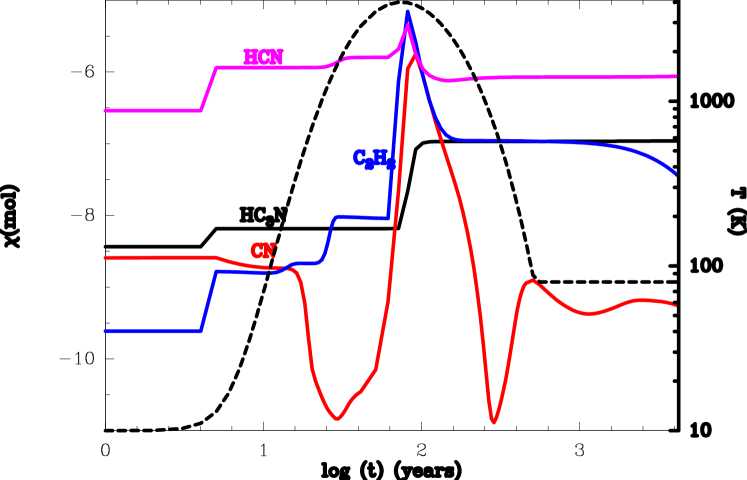
Figure 8: Modelling of HC₃N (black) and its potential precursors HCN (magenta), C₂H₂ (blue) and CN (red), in L1157-B1. The temperature profile across the shock is displayed with the black dashed line.

In order to determine whether HC₃N arises in the shocked gas of the L1157-B1 cavity, we consider the best fit chemical and parametric shock model from previous works by our team (Viti et al. 2011, Lefloch et al. 2016, Holdship et al. 2016), namely one where the pre-shock density is $10^{5}\hbox{\kern 1.99997ptcm${}^{-3}$}$ and the shock velocity is $40\hbox{\kern 1.99997ptkm\kern 1.99997pts${}^{-1}$}$. In Fig. 8, we plot the fractional abundance of HC₃N, and other selected species, as a function of time. We find that the abundance of HC₃N increases at two different times: the first increase is due to mantle sputtering due to the passage of the shock. The second increase is in fact due to the reaction of CN with C₂H₂: CN + C₂H₂ $\rightarrow$ HC₃N + H. This channel has an increased efficiency when the temperature is much higher than $300\hbox{\kern 1.99997ptK}$ due to the dependence of this reaction to temperature (Woon & Herbst 1997) but, most importantly, due to the enhanced C₂H₂ and CN abundances when the temperature is at its maximum ($\sim 4000\hbox{\kern 1.99997ptK}$). Indeed C₂H₂ and CN form via neutral-neutral reactions whose efficiency increases with temperature. In summary, the HC₃N abundance increases strongly as a consequence of the passage of the shock; this is consistent with the fact that observationally HC₃N appears to be enhanced (by a factor of 30) towards the shocked position of L1157-B1. Our modelling shows that the HC₃N abundance enrichment is dominated by the high-temperature gas phase reactions rather than sputtering of frozen HC₃N onto dust grains. This is consistent with the absence of differential fractionation between the three rare ¹³C isotopologues and the low deuterium enrichment when compared with the envelope of L1157-mm.

8 Conclusions

As part of ASAI, we have carried out a systematic search for cyanopolyynes HC_2n+1N towards the protostellar outflow shock region L1157-B1 and the protostar L1157-mm, at the origin of the outflow phenomenon. Towards L1157-B1, we confirm the detection of HC₃N lines $J$= 8–7 to $J$=29–28 and we report the detection of transitions from its ¹³C isotopologues $J$=9–8 to $J$=12–11. We have detected the HC₅N lines $J$=30–29 to $J$=43–42 for the first time in a shock. Towards L1157-mm, we detected the HC₃N lines $J$= 8–7 to $J$=28–27 and the deuterated isotopologue DC₃N lines $J$=9–8 to $J$=18–17. We summarize our main results as follows:

• The abundance of HC₃N has been increased by a factor of about 30 in the passage of the shock.

• The upper limit we can place on the deuterium fraction ratio D/H in the shock (0.002) shows that the abundance enhancement of HC₃N was not accompanied by a significant abundance enhancement of DC₃N, which is consistent with a warm gas phase formation scenario. This is also supported by the observed lack of ¹³C fractionation of HC₃N.

• The rather low abundance ratio X(HC₃N)/X(HC₅N) measured in L1157-B1 suggests that HC₅N was also efficiently formed in the shock.

• A simple modelling based on the shock code of Viti et al. (2011) and the chemical code UCL_CHEM, adopting the best fit solution determined from previous work on L1157-B1 by our team, accounts for the above observational results. The HC₃N abundance increases in a first step as a result of grain mantle sputtering and, in a second step, as a result of the very efficient gas phase reaction of CN with C₂H₂.

Appendix A Cyanopolyyne emission in L1157-mm

Table 6: Spectroscopic and observational parameters of the lines from HC₃N and its isotopologues identified towards the protostar L1157-mm. We give in bracket the statistical uncertainties on the observational parameters, as derived from a gauss fit to the profiles.

Transition	Frequency	$E_{u}$	$A_{ul}$	HPBW	$\eta_{mb}$	$\int T_{mb}dv$	FWHM	$V_{lsr}$
$J\rightarrow J-1$	MHz	K	s-1	′′		mK km s-1	km s-1	km s-1
HC3N
8 – 7	72783.822	15.7	2.94(-5)	33.8	0.86	338(4)	2.3(0.8)	3.0(0.1)
9 – 8	81881.468	19.7	4.21(-5)	30.0	0.85	305(4)	1.7(0.7)	2.3(0.1)
10 – 9	90979.023	24.0	5.81(-5)	27.0	0.84	330(4)	1.7(0.6)	2.9(0.1)
11 – 10	100076.392	28.8	7.77(-5)	24.6	0.84	264(7)	1.5(0.6)	2.8(0.1)
12 – 11	109173.634	34.1	1.01(-4)	22.5	0.83	267(7)	1.4(0.5)	2.4(0.1)
14 – 13	127367.666	45.9	1.62(-4)	19.3	0.81	189(8)	1.3(0.5)	2.5(0.1)
15 – 14	136464.411	52.4	1.99(-4)	18.0	0.81	178(9)	1.4(0.4)	2.6(0.1)
16 – 15	145560.960	59.4	2.42(-4)	16.9	0.79	141(9)	1.1(0.4)	2.5(0.1)
17 – 16	154657.284	66.8	2.91(-4)	15.9	0.77	113(19)	1.1(0.4)	2.7(0.1)
18 – 17	163753.389	74.7	3.46(-4)	15.0	0.77	99(12)	1.4(0.4)	2.5(0.1)
23 – 22	209230.234	120.5	7.26(-4)	11.8	0.67	72(9)	1.5(0.2)	2.5(0.1)
24 – 23	218324.723	131.0	8.26(-4)	11.3	0.65	31(10)	1.5(0.5)	2.8(0.2)
27 – 26	245606.320	165.0	1.18(-3)	10.0	0.62	27(10)	0.9(0.2)	2.2(0.1)
28 – 27	254699.500	177.3	1.32(-3)	9.7	0.60	20(12)	1.0(0.2)	1.1(0.1)
DC3N
9 – 8	75987.138	18.2	3.39(-5)	32.4	0.86	26(6)	2.7(1.3)	1.8(0.5)
10 – 9	84429.814	22.3	4.67(-5)	29.8	0.85	29(6)	2.0(0.7)	2.5(0.3)
11 – 10	92872.375	26.7	6.24(-5)	26.4	0.84	25(4)	1.8(0.3)	2.9(0.1)
13 – 12	109757.133	36.9	1.04(-4)	22.4	0.83	31(11)	1.9(1.2)	2.1(0.5)
18 – 17	151966.372	69.3	2.78(-4)	16.2	0.77	19(3)	1.3(0.2)	0.4(0.1)
HC5N
31 – 30	82539.039	63.4	6.04(-5)	29.8	0.85	36(8)	1.5(0.5)	3.5(0.2)
32 – 31	85201.346	67.5	6.64(-5)	28.9	0.85	27(5)	2.0(0.7)	2.5(0.3)
34 – 33	90525.889	76.0	7.98(-5)	27.2	0.85	14(2)	1.7(0.4)	2.4(0.2)
40 – 39	106498.910	104.8	1.30(-4)	23.1	0.84	13(2)	1.3(0.1)	2.5(0.1)

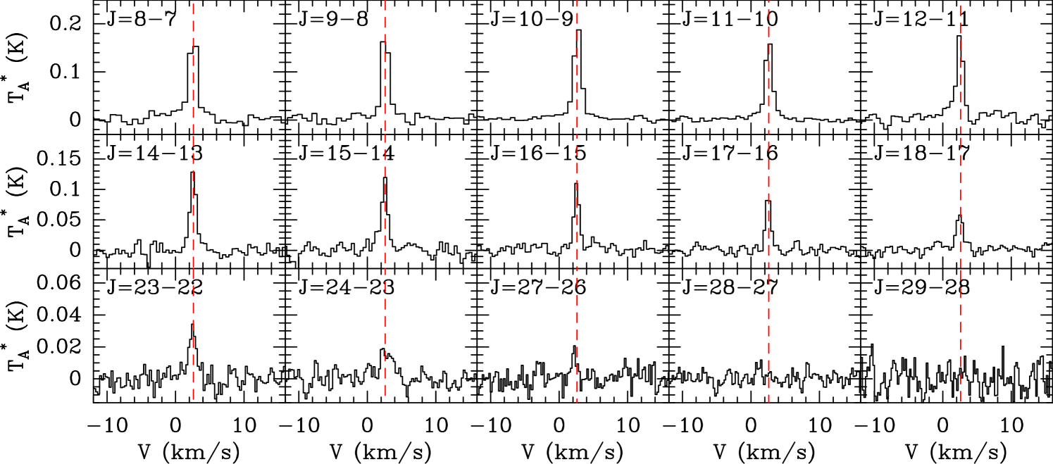
Figure 9: Montage of some HC₃N lines detected towards L1157-mm.

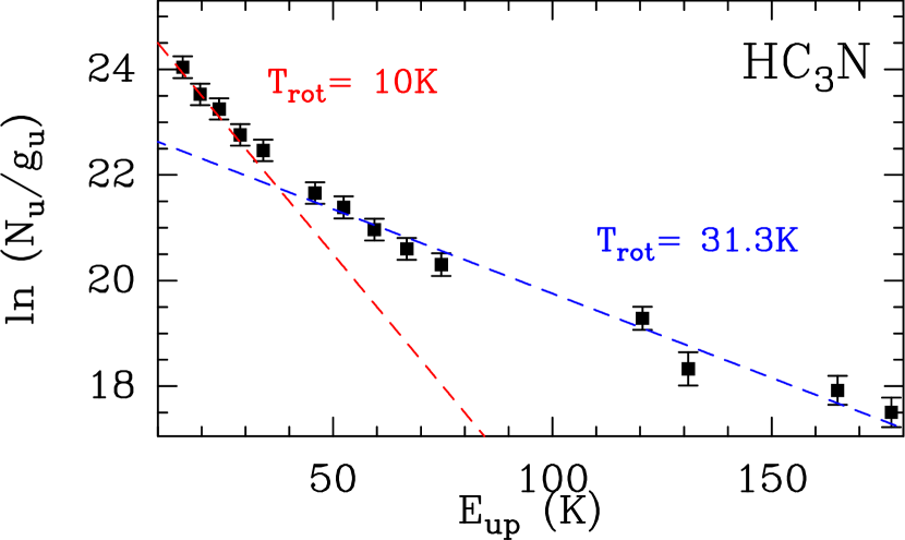
Figure 10: Rotational diagram analysis of HC₃N lines detected towards L1157-mm. The emission was corrected for the coupling between the source and the telescope beam assuming a typical size of $20\arcsec$ for the protostellar envelope. The fits to the two physical components accounting for the emission are shown in red and blue, respectively. In red, the cold component at $T_{rot}$= $10.0\pm 0.3\hbox{\kern 1.99997ptK}$ and N(HC₃N)= $(5.3\pm 0.6)\times 10^{12}\hbox{\kern 1.99997ptcm${}^{-2}$}$; in blue, the warmer component at $T_{rot}$= $31.3\pm 1.2\hbox{\kern 1.99997ptK}$ and N(HC₃N)= $(7.2\pm 1.0)\times 10^{12}\hbox{\kern 1.99997ptcm${}^{-2}$}$.

Figure 11: Montage of some DC₃N lines detected towards L1157-mm. We have superposed in red the best LTE fit to the emission with $T_{rot}$= $22.5\pm 1.6\hbox{\kern 1.99997ptK}$ and N(DC₃N)= $(3.4\pm 0.5)\times 10^{11}\hbox{\kern 1.99997ptcm${}^{-2}$}$ and a source size of $20\arcsec$.

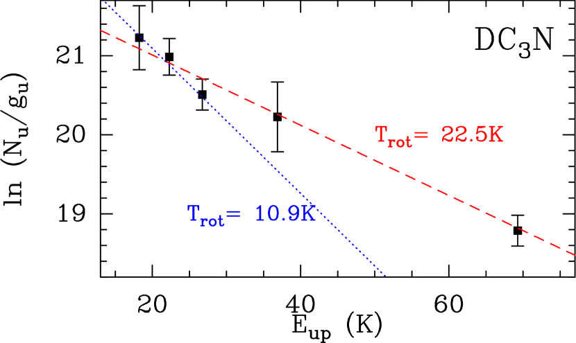
Figure 12: Rotational diagram analysis of DC₃N emission. The emission was corrected for the coupling between the source and the telescope beam assuming a typical size of $20\arcsec$. The best fit (dashed red line) is obtained for $T_{rot}$= $22.5\pm 1.6\hbox{\kern 1.99997ptK}$ and N(DC₃N)= $(3.4\pm 0.5)\times 10^{11}\hbox{\kern 1.99997ptcm${}^{-2}$}$. The fit obtained when considering only the data in the $E_{up}<40\hbox{\kern 1.99997ptK}$ range yields $T_{rot}$= $10.9\pm 1.7\hbox{\kern 1.99997ptK}$ and N(DC₃N)= $(5.2\pm 1.8)\times 10^{11}\hbox{\kern 1.99997ptcm${}^{-2}$}$; it is drawn by the blue dotted line.

References

- [Bachiller & Pérez Gutiérrez(1997)] Bachiller, R., Pérez Gutiérrez, M., 1997, ApJ, 487, L93
- [] Bachiller, R., Pérez Gutiérrez, M., Kumar, M. S. N., Tafalla, M., 2001, A&A, 372, 899
- [\citeauthoryearBell et al.1997] Bell, M. B., Feldman, P. A., Travers, M. J., McCarthy, M.C., Gottlieb, C.A., Thaddeus, P. 1997, ApJ, 483, L61
- [\citeauthoryearBenedettini et al.2012] Benedettini, M., et al. 2012, A&A, 539, L3
- [\citeauthoryearBenedettini et al.2013] Benedettini, M., et al. 2013, MNRAS, 436, 179
- [\citeauthoryearBusquet et al.2014] Busquet, G., et al., 2014, A&A, 561, 120
- [] Ceccarelli, C., et al., 2002, A&A, 383, 603
- [] Cernicharo, J., Guélin, M., 1996, A&A, 309, L27
- [] Chini, R., Ward-Thompson, D., Kirk, J.M., Nielbock, M., Reipurth, B., Sievers, A., 2001, A&A, 369, 155
- [] Clarke, D.W., Ferris, J.P., 1995, Icarus, 155, 119
- [\citeauthoryearCodella et al.2010] Codella, C., et al. 2010, A&A, 518, L112
- [\citeauthoryearCodella et al.2012] Codella, C., et al., 2012, ApJ, 757, L9
- [\citeauthoryearCodella et al.2015] Codella, C., Fontani, F., Ceccarelli, C., Podio, L., Viti, S., Bachiller, R., Benedettini, M., Lefloch, B., 2015, MNRAS, 449, L11
- [] Codella, C., et al., 2017, A&A, 605, L3
- [\citeauthoryearCordiner et al.2011] Cordiner, M. A., Charnley, S. B., Wirström, E.S., Smith, R.G., 2012, ApJL, 744, 131
- [\citeauthoryearCouepaud et al.2006] Couepaud A., Kolos, R., Couturier-Tamburelli, I., et al. 2006, J. Phys. Chem. A, 110, 2371
- [\citeauthoryearCrovisier et al.2004] Crovisier, J., et al., 2004, A&A, 418, 1141
- [] Faure, A., Lique, F., Wiesenfeld, L., 2016, MNRAS, 460, 2103
- [] Fontani,F., et al., 2017, A&A, 605, 57
- [] Friesen, R.K., Medeiros, L., Schnee, S., Bourke, T.L., Francesco, J.Di, Gutermuth, R., Myers, P.C., 2013, MNRAS, 436, 1513
- [\citeauthoryearGómez-Ruiz et al.2015] Gómez-Ruiz, A. I., et al. 2015, MNRAS, 446, 3346
- [\citeauthoryearGueth, Guilloteau, & Bachiller1996] Gueth, F., Guilloteau, S., & Bachiller, R. 1996, A&A, 307, 891
- [\citeauthoryearGueth, Guilloteau, & Bachiller1998] Gueth, F., Guilloteau, S., Bachiller, R. 1998, A&A, 333, 287
- [] Holdship, J., et al., 2016, MNRAS, 463, 802
- [] Jaber Al-Edhari, A., et al., 2017, A&A, 597, 40
- [\citeauthoryearLefloch et al.2010] Lefloch, B., et al. 2010, A&A, 518, L113
- [\citeauthoryearLefloch et al.2012] Lefloch, B., et al. 2012, ApJL, 757, L25
- [\citeauthoryearLefloch et al.2016] Lefloch, B., et al., 2016, MNRAS, 462, 3937
- [\citeauthoryearLefloch et al.2017] Lefloch, B., Ceccarelli, C., Codella, C., Favre, C., Podio, L., Vastel, C., Viti, S., Bachiller, 2017, MNRAS, 469, L73
- [\citeauthoryearLooney, Tobin & Kwon2007] Looney, L., Tobin, J., Kwon, W. 2007, ApJ, 670, L131
- [] Mendoza, E., Lefloch, B., López-Sepulcre, A., Ceccarelli, C., Codella, C., Boechat-Roberty, H.M., Bachiller, R., 2014, MNRAS, 445, 151
- [\citeauthoryearPodio et al.2014] Podio, L., Lefloch, B., Ceccarelli, C., Codella, C., Bachiller, R., 2014, A&A, 565, A64
- [\citeauthoryearPodio et al.2016] Podio, L., et al. 2016, A&A, 593, L4
- [\citeauthoryearPodio et al.2017] Podio, L., et al., 2017, MNRAS, 470, L16
- [\citeauthoryearSakai et al.2008] Sakai, N., Sakai, T., Hitora, T., Yamamoto,S., 2008, ApJ, 672, 371
- [] Tafalla, M., Bachiller, R., 1995, pJ, 443, L37
- [\citeauthoryearTafalla et al.2015] Tafalla, M., Bachiller, R., Lefloch, B., Rodríguez-Fernández, N., Codella, C., López-Sepulcre, A., Podio, L., 2015, A&A, 573, L2
- [\citeauthoryearTakano et al.1998] Takano, S., et al., 1998, A&A, 329, 1156
- [\citeauthoryearTakano et al.2014] Takano, S., et al., 2014, PASJ, 66, 75
- [] Viti, S., Jiménez-Serra, I., Yates, J. A., Codella, C., Vasta, M., Caselli, P., Lefloch, B., Ceccarelli, C., 2011, ApJ, 740, L3
- [] Yamaguchi, T., et al., 2012, PASJ, 64, 105
- [\citeauthoryearWoon & Herbst1997] Woon, D. E., & Herbst, E. 1997, ApJ, 477, 204