Insufficiency of avoided crossings for witnessing large-scale quantum coherence in flux qubits

Abstract

Do experiments based on superconducting loops segmented with Josephson junctions (e.g., flux qubits) show macroscopic quantum behavior in the sense of Schrödinger’s cat example? Various arguments based on microscopic and phenomenological models were recently adduced in this debate. We approach this problem by adapting –to flux qubits– the framework of large-scale quantum coherence, which was already successfully applied to spin ensembles and photonic systems. We show that contemporary experiments might show quantum coherence more than one hundred times larger than experiments in the classical regime. However, we argue that the often used demonstration of an avoided crossing in the energy spectrum is not sufficient to conclude about the presence of large-scale quantum coherence. Alternative, rigorous witnesses are proposed.

I Introduction

The experimental demonstration of a massive object in a superposition of two well separated positions is generally considered as a positive test of quantum mechanics on large scales. Typical examples are interference of large molecules or proposed experiments with levitating nanospheres Arndt and Hornberger (2014). These situations are often compared to Schrödinger’s thought experiment of a cat in a superposition of dead and alive Schrödinger (1935).

It was argued that superconducting quantum interference devices (SQUIDs), that is, superconducting loops segmented with Josephson junctions, can exhibit a similar characteristic Leggett (1980, 2002). In certain parameter regimes, the magnetic flux through the loop can be seen as an appropriate analog to the position of a massive object, where the capacitance of the circuit plays the role of the mass (see Fig. 1). The nonlinearity of the Josephson junction can lead to an effective double-well potential, in which the minima of the wells correspond to well separated (i.e., “macroscopically distinct”) flux states.

There has been a debate about the precise implications of successfully demonstrating a coherent superposition between the two wells Leggett (2002); Korsbakken et al. (2009, 2010); Leggett (2016); Björk and Mana (2004); Marquardt et al. (2008); Nimmrichter and Hornberger (2013). On the one hand, it was argued that recent experiments Friedman et al. (2000); van der Wal et al. (2000); Hime et al. (2006) operate in the 100 nA or $\mu$A regime implying the presence of up to $10^{9}$ electrons. This, together with the experimental evidence of “macroscopic coherence”, should be seen as a genuine “macroscopic quantum effect” Leggett (2002). On the other hand, arguments based on microscopic modeling suggest that effectively at most a few thousand electrons make the difference between the two states localized in each well Korsbakken et al. (2009, 2010) (see Leggett (2016) for a critique of this argument). Further contributions also assign an “effective size”, that is, a number that should, for example, reflect the number of electrons that effectively participate in the observed quantum effect Björk and Mana (2004); Marquardt et al. (2008); Nimmrichter and Hornberger (2013) (see also table 1). While the differences in the precise frameworks of Leggett (2002); Korsbakken et al. (2009, 2010); Leggett (2016); Björk and Mana (2004); Marquardt et al. (2008); Nimmrichter and Hornberger (2013) are expected to lead to some deviation in the obtained results, it is astonishing by how much they vary. We find effective sizes ranging from two Marquardt et al. (2008) to 10¹⁰ Leggett (2002). In addition, none of the theory papers present a conclusive, testable witness for their claim.

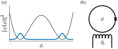
Figure 1: (a) Schematics of a superposition in the flux coordinate $\phi$ in both wells (thick: probability distribution; thin: potential). Experiments witnessing coherence between the two wells are sometimes considered to resemble a Schrödinger-cat situation if the inter-well distance and the system size (e.g., number of participating electrons) are large. (b) Most basic schematics of a superconducting ring with a single Josephson junction (cross; see also Sec. III). In a certain parameter regime the magnetic flux $\phi$ through the ring is an appropriate choice for the relevant degree of freedom Friedman et al. (2000); van der Wal et al. (2000); Leggett (2002); Caldeira (2014). The SQUID is then called flux qubit. The external flux $\phi_{x}$ controls the effective potential for $\phi$. In practice, the single Josephson junction is replaced by several junctions for an in situ control of some experimental parameters Friedman et al. (2000); van der Wal et al. (2000); Hime et al. (2006).

In this paper, we argue that one important aspect of the large-scale quantum nature of these experiments is the amount and the spread of quantum coherence in the flux coordinate since it is a direct test of the superposition principle. As already successfully done for spins and photons Fröwis and Dür (2012); Fröwis et al. (2015); Oudot et al. (2015), we rescale the coherence of the target state by the coherence of a classical reference state (i.e., the state confined in a single well). In this way, we introduce an “effective size” that quantifies the scale of the quantum effect. The advantage of this approach is the applicability to experimental data.

After a short review of the motivation and the theory of the framework in Sec. II, the phenomenological model of the flux qubit experiments is presented in Sec. III. Identifying the flux as a relevant observable, we show that indeed the ideally generated target states show large quantum coherence. With the parameters from experiment Friedman et al. (2000), we find that the quantum coherence of the target states in flux basis is almost two hundred times larger than of a classical reference state (i.e., the ground state of a single potential well). Ideal cat states could even reach numbers 1000 times larger than that of the reference state.

The experimental proof for the generation of the eigenstates was argued to be the avoided crossing in the energy spectrum when tuning the imbalance of the two well minima. In Sec. V, we show that this evidence is not sufficient to conclude the presence of large-scale quantum coherence. We do so by presenting a simple dephasing model in the flux basis that leads to a drastic reduction of the quantum coherence (to the level of the classical reference state) while keeping the feature of the avoided crossing.

The framework of large-scale quantum coherence provides testable witnesses, which often turn out to be feasible in practice Fröwis (2017). In Sec. V.2, we discuss the possibility of lower-bounding large quantum coherence by witnessing a strong response of the system to flux dephasing. The paper is summarized and discussed in Sec. VI.

II Framework of large quantum coherence

One of the simplest and most fundamental questions in quantum mechanics is the validity of the superposition principle on all scales. There exist several alternative models that, for example, prevent a persistent superposition of two significantly distinct positions for massive particles Bassi et al. (2013). Given an observable $X$ with a natural macroscopic limit (such as position or magnetization), quantum coherence between two far-distant parts of the spectrum arguably challenges our classical intuition more than quantum coherence constraint to a small (microscopic) regime Schrödinger (1935).

For pure states, a superposition between far-distant spectral parts of $X$ implies that the wave function has a large spread. The simplest way to measure the spread of a state $|\psi\rangle$ is the variance $\mathrm{var}_{\psi}(X)$. For mixed states, the variance is no longer a faithful measure of coherence since it does not distinguish between coherent superposition and incoherent mixture. The convex roof construction is a well-known technique to overcome the shortcomings of the variance. Given a mixed state $\rho$, one considers the infinite set of all pure state decompositions (PSD) $\rho=\sum_{i}p_{i}\left|\psi_{i}\right\rangle\!\left\langle\psi_{i}\right|$ and minimizes the average variance

$$\mathcal{I}(\rho,X)=\min_{\mathrm{PSD}}\sum_{i}p_{i}\mathrm{var}_{\psi_{i}}(X).$$ (1)

Since the incoherent part is eliminated with the convex roof construction, we call $\mathcal{I}(\rho,X)$ the quantum coherence of $\rho$ in the spectrum $X$. Measuring a certain value of $\mathcal{I}$ experimentally falsifies all collapse models that forbid the superposition principle to be valid on the order of $\sqrt{\mathcal{I}}$.

Notably, $4\mathcal{I}$ is the so-called quantum Fisher information Helstrom (1976); Braunstein and Caves (1994); Yu (2013). This implies that large quantum coherence is necessary to reach high sensitivity in parameter estimation protocols where $X$ is the generator of the parameter shift. The intuitive motivation to choose the convex roof of the variance is made more rigorous in a recent resource theory of “macroscopic coherence” Yadin and Vedral (2016).

It arguably makes sense to compare $\mathcal{I}(\rho,X)$ to a reference state $|\psi_{\mathrm{ref}}\rangle$, which behaves “maximally” classically among all pure quantum states. Like the choice for the observable $X$, identifying $|\psi_{\mathrm{ref}}\rangle$ is physically motivated and hence situation-dependent. Nevertheless it brings some conceptual advantages, as we can avoid unwanted dependencies on scaling factors of $X$. Furthermore, it helps to compare systems with various numbers of modes or particles. One defines

$$\mathcal{I}_{\mathrm{rel}}(\rho,X)=\frac{\mathcal{I}(\rho,X)}{\mathcal{I}(\psi_{\mathrm{ref}},X)},$$ (2)

which tells us how much larger the quantum coherence of $\rho$ is compared to that of the reference state.

The observable $X$ and the reference state have to be physically motivated. Let us consider two examples Fröwis and Dür (2012); Fröwis et al. (2015). Quadrature operators $X=e^{i\theta}a+e^{-i\theta}a^{\dagger}$ for phase space states (sums of quadrature operators for many modes) and collective spin operators $X=\sum_{i=1}^{N}\sigma^{(i)}$ proved to be reasonable choices. The reference states are the coherent state in phase space and the spin-coherent state (i.e., parallel spins in a product state) in spin ensembles, respectively. It was shown that $\mathcal{I}_{\mathrm{rel}}(\rho,X)$ can then be interpreted as an effective size as it is connected to the number of microscopic entities (photons or spins) that effectively contribute to the large-scale quantum effect Fröwis et al. (2017). Generally, let us consider a classical reference state composed of uncorrelated microscopic constituents (“particles”) and an additive observable with a macroscopic limit. Then the variance is linear in the number of particles $N$, that is, $\mathrm{var}(X)=N\overline{\mathrm{var}}(x_{0})$, where $x_{0}$ is the corresponding one-particle operator and $\overline{\mathrm{var}}$ is the average variance per particle. Then, the effective size $\mathcal{I}_{\mathrm{rel}}(\rho,X)$ gives the spread of the quantum coherence per particle and per microscopic unit, which justifies the use of the variance rather than, for example, the square root of it.

III Short summary of SQUID physics

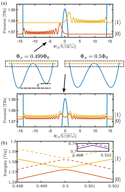
Figure 2: (a) Center: two examples of the double-well potential $U$ (curved, blue line; Eq. (3)) for $\Phi_{x}=0.499\Phi_{0}$ and $\Phi_{x}=0.5\Phi_{0}$. The difference $\epsilon$ between the two minima for $\Phi_{x}=0.499\Phi_{0}$ is artificially increased for a clearer distinction between the two cases. Top: absolute square of the wave functions of the target states $|0\rangle$ and $|1\rangle$ at $\Phi_{x}=0.499\Phi_{0}$ in the experiment of Ref. Friedman et al. (2000), shifted by the respective eigenenergy. The confinement of each in a single well is clearly visible. Bottom: The same at $\Phi_{x}=0.5\Phi_{0}$. The wave functions are both spread over both wells. (b) Energies of the target states as a function of $\Phi_{x}$ (solid lines). The avoid crossing at $\Phi_{x}=0.5\Phi_{0}$ is clearly visible. The dashed lines are the energies of the target states after dephasing as described in Eq. (7) with $\Gamma=\sqrt{\hbar/(C\omega)}$. The energies are shifted, but the avoided crossing is still present. The inset shows the energy of the ground state before (solid) and after (dashed) dephasing with the same $\Gamma$.

In the discussion on whether experiments with superconducting devices show aspects of a Schrödinger-cat state, some approaches Marquardt et al. (2008); Korsbakken et al. (2009, 2010) work with a microscopic model. This leads to discussions about details like the proper choice of the “microscopic unit” or of characteristic quantities Leggett (2016). In the presented approach based on quantum coherence $\mathcal{I}$, it is more natural to work with a phenomenological model of a single degree of freedom, the total flux $\Phi$ and the charge $Q$ as the conjugate variable (i.e., $[\Phi,Q]=i\hbar$). To discuss a specific example, let us consider the SQUID experiment of Friedman et al. Friedman et al. (2000). The effective potential depends on the the inductance $L$ and the critical current $I_{c}$. In addition, it is controlled by an external flux $\Phi_{x}$ (see Fig. 1 (b)). This results in a quadratic part with inductive energy $E_{L}=\Phi_{0}^{2}/(2L)$ and in a nonlinear part from the junction with Josephson coupling energy $E_{J}=I_{c}\Phi_{0}/(2\pi)$ ($\Phi_{0}$ is the magnetic flux quantum), that is,

$$U(\phi)=E_{L}\left(\frac{\Phi-\Phi_{x}}{\Phi_{0}}\right)^{2}+E_{J}\cos\left(2\pi\Phi/\Phi_{0}\right).$$ (3)

The Hamiltonian is completed by the “kinetic” energy $\frac{1}{2C}Q^{2}$ where $C$ is the capacitance. For later, we introduce the charging energy $E_{C}=e^{2}/(2C)$ and the angular frequency of the hypothetical $LC$ circuit, $\omega=1/\sqrt{LC}$. The experimental parameters given in Ref. Friedman et al. (2000) are $E_{C}=188$ MHz, $E_{L}=13$ THz and $E_{J}=159$ GHz. In the following we use these numbers when it comes to numeric calculations, but we generally assume $E_{J},E_{L}\gg E_{C}$.

Depending on $\Phi_{x}$, the potential $U$ can exhibit an effective double-well structure (see Fig. 2 (a)). At $\Phi_{x}=\frac{1}{2}\Phi_{0}$, there exist two global minima separated by roughly $0.655\Phi_{0}$. This implies that coherent tunneling is possible and the wave functions of the eigenstates have finite contributions in both wells. This leads to statements like “the wave function lives in both wells”. Given the large separation and the involvement of up to 10⁹ Cooper pairs, some physicists have called this a Schrödinger-cat situation. The “classical” regime is at $\Phi_{x}=0$, as the potential has a (deep) single well with a well-defined flux state as its ground state. While a small anharmonicity is always present, the ground state in this regime behaves like the ground state of an harmonic oscillator if $E_{L},E_{J}\gg E_{C}$. For example, the variance of $\Phi$ and $Q$ are minimal in the sense that the Heisenberg uncertainty relation is basically tight . Hence, this state is chosen as the reference state as it behaves most classically.

As argued in Refs. Friedman et al. (2000); Leggett (2002), the experimental proof of the coherent superposition of “left and right” is the resolution of the predicted avoided crossing by tuning the imbalance between left and right well (see Fig. 2 (a)). Since the energy gap is proportional to the tunneling probability, the splitting between the lowest two eigenstates is very tiny for the given energies. Hence the initial ground state is driven to highly excited states just below the barrier. There, the minimal energy gap is pronounced enough to be measurable (see Fig. 2 (b)).

While the discussion in this paper is adapted to the experiment of Ref. Friedman et al. (2000), other experimental setups lead to conceptually similar results. For example, the three-junction setup of van der Wal et al. van der Wal et al. (2000) can be modeled with two independent flux coordinates. A suitable coordinate transform leads to an effective double well potential similar to the one discussed before Orlando et al. (1999). Hence, we will find qualitative similar results, which are later given without discussing details. We only mention that a further parameter of the experiment is $\alpha$, which is the ratio of the Josephson coupling energy of one junction to the other two (identical) junctions. The parameters from Ref. van der Wal et al. (2000) are $E_{J}/E_{C}=38$ and $\alpha=0.8$.

IV Large quantum coherence in flux qubits

In this section, we apply the framework of large quantum coherence to the flux qubit. Following on the discussion in Sec. II, we choose a target state (i.e., the state which is supposed to exhibit large quantum coherence), an observable $X$ for which we evaluate the spread of coherence, and a classical reference state to which we want to compare the target state. From Sec. III, it is evident that eigenstates (e.g., ground states) at $\Phi_{x}=1/2\Phi_{0}$ are good candidates for “cat states” if we choose $X=\Phi$. The ground state at $\Phi_{x}=0$ serves as the classical reference state. In Sec. IV.1, we take the ground state at $\Phi_{x}=1/2\Phi_{0}$ as the target state, while in Sec. IV.2 we numerically analyze the target states of the experiment in Ref. Friedman et al. (2000). Since in both cases we treat the ideal situation, the quantum coherence $\mathcal{I}$ simplifies to the variance.

IV.1 Effective size of the ideal cat state

We first calculate the variance of the classical reference state. For this, we notice that we are in the regime $E_{L}/E_{C}\approx 7.17\times 10^{4}\gg 1$, which implies a rather deep potential in the classical situation $\Phi_{x}=0$. It can be easily shown that the anharmonic part of the potential does not significantly influence the ground state (despite a large $E_{J}$). Hence, to obtain an analytical result, we approximate $U$ from Eq. (3) by an harmonic oscillator. From the second-order Taylor series of $U$ at $\Phi_{x}=0$, we can extract the effective trapping frequency $\omega_{\mathrm{cl}}=\omega\sqrt{1+2\pi^{2}E_{J}/E_{L}}$ and find

$$\mathrm{var}_{\mathrm{ref}}(\Phi)\approx\frac{\hbar}{2C\omega_{\mathrm{cl}}}=\frac{1}{2\pi}\sqrt{\frac{E_{C}}{E_{L}+2\pi^{2}E_{J}}}\Phi_{0}^{2}.$$ (4)

We now turn to the ground state at $\Phi_{x}=\Phi_{0}/2$, which is an equally weighted superposition of being in the left and right well. For simplicity, this state is called “cat state” in the following. Since the distance $d$ between the minima is much larger than the spread of the wave packet in one well, we approximate the variance of the cat state by $d^{2}$. In the present parameter regime, $d$ is in the order of $\Phi_{0}$ with a slight dependency on $E_{C}$ and $E_{J}$. We numerically find $\mathrm{var}_{\mathrm{cat}}(\Phi)\approx 0.655^{2}\Phi_{0}^{2}$. Together with Eq. (4), we have

$$\mathcal{I}_{\mathrm{rel}}(\Phi)\approx 0.86\pi\sqrt{\frac{E_{L}+2\pi^{2}E_{J}}{E_{C}}}\approx 1315.$$ (5)

In the limit of a dominant Josephson energy $E_{J}/E_{L}\propto I_{c}L/\Phi_{0}\gg 1$ (while keeping $E_{L}\gg E_{C}$), one has $\mathrm{var}_{\mathrm{cat}}(\Phi)\approx\Phi_{0}^{2}$ and $\mathcal{I}_{\mathrm{rel}}\approx 2\sqrt{2}\pi^{2}\sqrt{E_{J}/E_{C}}\approx 2565$.

The calculation for the experiment of Ref. van der Wal et al. (2000) is analogous, but gives a fully analytic expression. We find

$$\mathcal{I}_{\mathrm{rel}}=4\arccos^{2}\left(\frac{1}{2\alpha}\right)\sqrt{4\alpha+2}\sqrt{\frac{E_{J}}{E_{C}}}\approx 45.$$ (6)

For both experiments, we note the scaling of the effective size with $\sqrt{{E_{J}}/{E_{C}}}$.

IV.2 Effective size of the target states of Ref. Friedman et al. (2000)

We now numerically calculate the effective size of $|0\rangle$ and $|1\rangle$ (see Fig. 2 (a)) that were targeted in the experiment of Ref. Friedman et al. (2000). For this, we first have to numerically diagonalize the Hamiltonian. As detailed in Ref. Everitt et al. (2004), one analytically calculates the eigenbasis of the Hamiltonian in the case of $E_{J}=0$ (since it reduces to the familiar $LC$ circuit) and then expresses the general $H$ in this basis. With the experimental parameters mentioned in Sec. III, we can diagonalize $H$ with high precision and reasonable cut-off dimensions.

Here, we are interested in the regime around $\Phi_{x}=\frac{1}{2}\Phi_{0}$. As shown in Fig. 2 (a), at $\Phi_{x}=\frac{1}{2}\Phi_{0}$, the wave functions are indeed spread over the entire classically allowed range. For the classical reference state, we again use Eq. (4). The eigenstate $|1\rangle$ exhibits a spread of $\mathrm{var}_{\left|1\right\rangle}(\Phi)\approx 6.32\times 10^{-2}\Phi_{0}^{2}$. We find $\mathcal{I}_{\mathrm{rel}}\approx 194$. For the second state $|0\rangle$, the spread is slightly smaller.

Table 1: Comparison of effective size $\mathcal{I}_{\mathrm{rel}}$ with results from literature for experiments Friedman et al. (2000); van der Wal et al. (2000). Our method is conceptually closest to the work of Björk and Mana Björk and Mana (2004), whose result has to be squared to match ours. Interestingly, we obtain similar numbers as Korsbakken et al. (2009) (in the scenario of Sec. IV.1) despite the different approach. See Sec. VI and Ref. Fröwis et al. (2017) for further discussion.

Reference	SUNY Friedman et al. (2000)	Delft van der Wal et al. (2000)
Effective size $\mathcal{I}_{\mathrm{rel}}$	1315 / 194	45
Leggett Leggett (2002)	$10^{10}/10^{10}$	$10^{6}/10^{10}$
Björk and Mana Björk and Mana (2004)	33	-
Marquardt et al. Marquardt et al. (2008)	-	$\lesssim 2$
Korsbakken et al. Korsbakken et al. (2009)	3800 - 5750	42

V Certifying large quantum coherence in experiments

We now turn to the question of how to certify the presence of large quantum coherence from the experimental data. We first show that the demonstration of an avoided crossing in the energy spectrum is not sufficient to witness wide-spread coherence. To this end we introduce a specific dephasing model that largely preserves the energy gap but significantly reduces the quantum coherence. Hence, we discuss alternative schemes at the end of the section.

V.1 Robustness of avoided crossing, fragility of quantum coherence

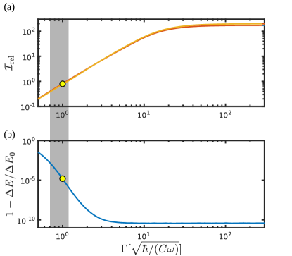
Figure 3: Impact of dephasing as a function of the correlation length $\Gamma$ for the two eigenstates $|0\rangle$ and $|1\rangle$ (see Sec. IV.2 and Fig. 2 (a)) at fixed $\Phi_{x}=\frac{1}{2}\Phi_{0}$. (a) The relative quantum coherence $\mathcal{I}_{\mathrm{rel}}$ drops quickly when increasing the dephasing strength (i.e., decreasing $\Gamma$). For $\Gamma\approx 4\sqrt{\mathrm{var}_{\mathrm{cl}}(\Phi)}$, one has $\mathcal{I}_{\mathrm{rel}}\approx 1$, that is, the spread of the quantum coherence is at the same order as the classical reference state. (b) Relative difference of the energy gap $\Delta E$ under dephasing ($\Delta E_{0}$ denotes the energy gap without dephasing). The energy gap $\Delta E$ is basically invariant for large $\Gamma$. Only for $\Gamma\lesssim 4\sqrt{\mathrm{var}_{\mathrm{cl}}(\Phi)}$ the relative difference becomes experimentally relevant. The gray zone highlights the parameter range of $\Gamma$ where $\mathcal{I}_{\mathrm{rel}}\leq 1$ and $1-\Delta E/\Delta E_{0}\leq 10^{-3}$. The yellow circles mark $\Gamma=\sqrt{\hbar/(C\omega)}$, which is also used in Fig. 2 (b). The relative difference saturates at around 10^-10 for large $\Gamma$ because of numerical precision.

In this section, we consider a simple dephasing model in the flux basis and discuss its consequences. Suppose that the eigenstates are subject to dephasing

$$\rho(\Phi,\Phi^{\prime})\rightarrow e^{-(\Phi-\Phi^{\prime})^{2}/(2\Gamma^{2})}\rho(\Phi,\Phi^{\prime}),$$ (7)

meaning that coherence-elements $\rho(\Phi,\Phi^{\prime})$ are damped by a Gaussian function on a scale $\Gamma$ (called correlation length in the following). From the discussion in Sec. II it is not surprising that this map reduces the quantum coherence $\mathcal{I}$, which is calculated using the spectral decomposition $\rho=\sum_{i}\lambda_{i}\left|\psi_{i}\right\rangle\!\left\langle\psi_{i}\right|$ and

$$\mathcal{I}(\rho,\Phi)=\sum_{i<j}\frac{(\lambda_{i}-\lambda_{j})^{2}}{\lambda_{i}+\lambda_{j}}\left|\left\langle\psi_{i}\right|\Phi\left|\psi_{j}\right\rangle\right|^{2}$$ (8)

(see, e.g., Ref. Braunstein and Caves (1994)). The result for $\Phi_{x}=\frac{1}{2}\Phi_{0}$ and variable $\Gamma$ is presented in Fig. 3, which shows the fragility of the quantum coherence under flux dephasing. In contrast, the energy gap $\Delta E$ (i.e., the difference in the energy expectation value between the dephased eigenstates at $\Phi_{x}=\frac{1}{2}\Phi_{0}$) is rather stable (see Fig. 3 (b)). Only for a correlation length $\Gamma\lesssim\sqrt{\hbar/(C\omega)}$ (i.e., close to the width of the classical reference state) $\Delta E$ deviates significantly from the energy gap between the original eigenstates, denoted by $\Delta E_{0}$. Note that the energies of the states are increased by the map (7). Since this affects all states equally strong (including the ground state), the differences in energies remain basically unchanged.

From these findings, we conclude that the mere observation of an avoided crossing is not sufficient to prove large quantum coherence in the system. We emphasize that this conclusion cannot be found by reducing the flux coordinate to a two-dimensional space (left well/ right well), which is often done in qualitative discussions.

V.2 Sufficient experimental test

We now discuss the possibility for a sufficient experimental test to certify a minimal quantum coherence $\mathcal{I}(\rho,\Phi)$. As shown in Ref. Fröwis et al. (2016), we can employ the following dynamical protocol. For this, we have to be able to implement $V_{t}=\exp(-i\Phi t)$. We first choose a suitable measurement with measurement operators $\{\Pi_{k}\}$ for the outcomes $\{x_{k}\}$. Then, we measure the probability distributions $p_{k}=\mathrm{Tr}\rho\Pi_{k}$ and $q_{k}=\mathrm{Tr}V_{t}\rho V_{t}^{\dagger}\Pi_{k}$. With this, we calculate the so-called Bhattacharyya coefficient $B=\sum_{k}\sqrt{p_{k}q_{k}}$. One finds Fröwis et al. (2016)

$$\mathcal{I}(\rho,\Phi)\geq\frac{1}{t^{2}}\arccos^{2}B.$$ (9)

In essence, inequality Eq. (9) witnesses the response of the system to a dynamical process generated by $\Phi$. High susceptibility implies the presence of large-scale quantum coherence. Using this bound, one finds certified quantum coherence which is (in the cold atom experiment of Ref. Hosten et al. (2016), for example) up to $71$ larger than that of classical reference states Fröwis (2017).

As we show now, we can relax the requirements of this protocol. For instance, suppose we are not able to fully control $t$ (i.e., the duration of the unitary), but we only assume that $t$ follows a certain distribution $\mu(t)$ with $\int dt\mu(t)=1$. Then, the quantum state after the non-unitary dynamics is described by

$$\mathcal{E}(\rho)=\int_{-\infty}^{\infty}dt\mu(t)V_{t}\rho V_{t}^{\dagger}.$$ (10)

For example,

$$\mu(t)=\frac{1}{\sqrt{2\pi}\Gamma}\exp(-\Gamma^{2}t^{2}/2)$$ (11)

leads to an effective dephasing in the $\Phi$ basis exactly as modeled in Eq. (7). We redefine $q_{k}=\mathrm{Tr}\mathcal{E}(\rho)\Pi_{k}$ for the calculation of $B$. Following Ref. Fröwis et al. (2016) and using the quantum fidelity $F$, one can show that

$$\begin{split}B&\geq F(\rho,\mathcal{E}(\rho))\geq\int_{-\infty}^{\infty}dt\mu(t)F(\rho,V_{t}\rho V_{t}^{\dagger})\\ &\geq\int_{-\pi/(2\sqrt{\mathcal{I}})}^{\pi/(2\sqrt{\mathcal{I}})}dt\mu(t)\cos\left(\sqrt{\mathcal{I}}t\right),\end{split}$$ (12)

where for the last step we used $F(\rho,V_{t}\rho V_{t}^{\dagger})\geq\cos\left(\sqrt{\mathcal{I}}t\right)$ in the interval $t\in[-\pi/(2\sqrt{\mathcal{I}}),\pi/(2\sqrt{\mathcal{I}})]$ Uhlmann (1991); Fröwis (2012). Finally, one has to invert inequality (12) to obtain a lower bound on the quantum coherence $\mathcal{I}$. This is generally not analytically possible, but one can find either numerical solutions or approximations. The numerical solution is an optimization problem where one finds the maximal $\mathcal{I}$ such that the inequality in Eq. (12) is fulfilled given the data, $B$, and the model of the dynamics, $\mu(t)$. As an example for an analytical approximation, we consider Eq. (11). In the weak dephasing limit (i.e., $\Gamma^{2}\gg\mathcal{I}$), we can safely move the integration limits in the second line of Eq. (12) from $\pm\pi/(2\sqrt{\mathcal{I}})$ to $\pm\infty$, which allows us to find $B\gtrsim\exp(-\Gamma^{2}\mathcal{I}/2)$, from which

$$\mathcal{I}(\rho,\Phi)\gtrsim 2\Gamma^{2}\log 1/B$$ (13)

follows.

Recent experiments with flux qubits (e.g., by Knee et al. Knee et al. (2016)) are conceptually and technically very close to the presented framework. A standard way of implementing measurements is based on the Josephson Bifurcation Amplifier Siddiqi et al. (2004); Lupaşcu et al. (2007); Nakano et al. (2009), which can be modeled by a dephasing process similar to Eq. (10). This opens the opportunity for witnessing large quantum coherence with flux qubits. Then, the protocol in Ref. Knee et al. (2016), which was employed to falsify so-called macrorealistic theories, is of the same spirit as the procedure presented here, namely to witness the susceptibility of a system with respect to a specific influence. The difference is that here we do need to control the experiment to a certain degree. In particular, the dynamics of Eq. (10) should be well characterized (e.g., $\Gamma$ in Eq. (11) should be sufficiently known), while assumptions on the initial state $\rho$ and the measurement $\{\Pi_{k}\}$ are not necessary.

VI Discussion and summary

In this paper, we proposed to consider the extent of quantum coherence in the flux coordinate as one relevant aspect of the “macroscopic quantum nature” of flux qubits. While the framework of large quantum coherence arguably has an operational meaning in the resource theory of asymmetry Marvian and Spekkens (2016); Yadin and Vedral (2016) and metrology Helstrom (1976); Braunstein and Caves (1994), its interpretation as an “effective size” (i.e., how many Cooper pairs or electrons effectively contribute to the quantum phenomenon) is less clear.

From a mathematical point of view, the framework of large quantum coherence is directly applicable to the SQUID experiments. The choice of observable (here, the flux $\Phi$) and the reference state (ground state of the “classical” regime $\Phi_{x}=0$) are physically motivated. The scaling of the effective size in the ideal case (Sec. IV.1) with $\sqrt{E_{J}/E_{C}}$ is interesting as the ratio $E_{J}/E_{C}$ is sometimes argued to be the relevant scale of the experiment Marquardt et al. (2008).

In this context, it is interesting to compare our results with the analysis by Korsbakken et al. Korsbakken et al. (2009, 2010) . The authors work with a microscopic model to investigate the effective number of participating Cooper pairs in the cat state. They find numbers around 3800 - 5750 for Ref. Friedman et al. (2000) and 42 for Ref. van der Wal et al. (2000). Since their results depend on experimentally “difficult” quantities like the Fermi velocity, this work was criticized by Leggett in Ref. Leggett (2016) where he constructs an “obvious” example of a Schrödinger-cat state that still gives a very low effect size with Korsbakken et al.’s method. Nevertheless, we note that our results (which only depend on the phenomenological model) and the results of Korsbakken et al. are in the same order. It would be interesting to see whether this is pure coincidence or whether there is some underlying connection.

We have shown that the experimental observation of avoided crossing in the energy spectrum is not a conclusive witness for the presence of large-scale quantum coherence. In contrast, the framework of large quantum coherence provides powerful lower bounds that are testable in practice. Here, we extended a recently developed protocol Fröwis et al. (2016) to nonunitary dynamics, which is conceptually and technically close to existing experiments Knee et al. (2016). Note that Eq. (12) is a general way to lower bound the spread of quantum coherence for an observable $X$. For its successful application, it is necessary to faithfully implement the unitary $V_{t}=\exp(-itX)$ in the experiment and to observe the impact by measuring the system before and after its application (on different runs). The control of $t$ can be relaxed to having knowledge about its distribution over many runs, $\mu(t)$. In contrast, no knowledge about the measurement is necessary to guarantee the correctness of Eq. (12).

The presented work gives a first insight that wide-spread quantum coherence might be present in SQUID experiments. We see our results as a starting point for further investigations. As mentioned before, the microscopical interpretation of $\mathcal{I}_{\mathrm{rel}}$ is open. Furthermore, one should apply the framework of large quantum coherence to other experiments and parameter regimes, such as $E_{J}>E_{C}>E_{L}$ (i.e., fluxonium) and $E_{J}\approx E_{L}\gg E_{C}$ (c-shunt flux qubit). A well-justified choice of the relevant observable as well as the target and reference state will lead to further insight to meso- and macroscopic quantum phenomena.

Acknowledgments.— We thank Daniel Estève and his research team, Amir Caldeira, Bill Munro, George Knee, Pavel Sekatski and Wolfgang Dür for inspiring discussions. This work was supported by the National Swiss Science Foundation (SNF), grant No. 172590, the European Research Council (ERC MEC), the EPSRC and Wolfson College, University of Oxford.

References

- Arndt and Hornberger (2014) M. Arndt and K. Hornberger, Nat Phys 10, 271 (2014).
- Schrödinger (1935) E. Schrödinger, Naturwissenschaften 23, 807 (1935).
- Leggett (1980) A. J. Leggett, Progress of Theoretical Physics Supplement 69, 80 (1980).
- Leggett (2002) A. J. Leggett, Journal of Physics: Condensed Matter 14, R415 (2002).
- Korsbakken et al. (2009) J. I. Korsbakken, F. K. Wilhelm, and K. B. Whaley, Phys. Scr. 2009, 014022 (2009).
- Korsbakken et al. (2010) J. I. Korsbakken, F. K. Wilhelm, and K. B. Whaley, EPL 89, 30003 (2010).
- Leggett (2016) A. J. Leggett, arXiv:1603.03992 [quant-ph] (2016).
- Björk and Mana (2004) G. Björk and P. G. L. Mana, J. Opt. B: Quantum Semiclass. Opt. 6, 429 (2004).
- Marquardt et al. (2008) F. Marquardt, B. Abel, and J. von Delft, Phys. Rev. A 78, 012109 (2008).
- Nimmrichter and Hornberger (2013) S. Nimmrichter and K. Hornberger, Phys. Rev. Lett. 110, 160403 (2013).
- Friedman et al. (2000) J. R. Friedman, V. Patel, W. Chen, S. K. Tolpygo, and J. E. Lukens, Nature 406, 43 (2000).
- van der Wal et al. (2000) C. H. van der Wal, A. C. J. ter Haar, F. K. Wilhelm, R. N. Schouten, C. J. P. M. Harmans, T. P. Orlando, S. Lloyd, and J. E. Mooij, Science 290, 773 (2000).
- Hime et al. (2006) T. Hime, P. A. Reichardt, B. L. T. Plourde, T. L. Robertson, C.-E. Wu, A. V. Ustinov, and J. Clarke, Science 314, 1427 (2006).
- Caldeira (2014) A. O. Caldeira, An Introduction to Macroscopic Quantum Phenomena and Quantum Dissipation (Cambridge University Press, 2014).
- Fröwis and Dür (2012) F. Fröwis and W. Dür, New Journal of Physics 14, 093039 (2012).
- Fröwis et al. (2015) F. Fröwis, N. Sangouard, and N. Gisin, Optics Communications 337, 2 (2015).
- Oudot et al. (2015) E. Oudot, P. Sekatski, F. Fröwis, N. Gisin, and N. Sangouard, Journal of the Optical Society of America B 32, 2190 (2015).
- Fröwis (2017) F. Fröwis, J. Phys. A: Math. Theor. 50, 114003 (2017).
- Bassi et al. (2013) A. Bassi, K. Lochan, S. Satin, T. P. Singh, and H. Ulbricht, Rev. Mod. Phys. 85, 471 (2013).
- Helstrom (1976) C. Helstrom, Quantum Detection and Estimation Theory (Academic Press, 1976).
- Braunstein and Caves (1994) S. L. Braunstein and C. M. Caves, Phys. Rev. Lett. 72, 3439 (1994).
- Yu (2013) S. Yu, arXiv:1302.5311 (2013).
- Yadin and Vedral (2016) B. Yadin and V. Vedral, Phys. Rev. A 93, 022122 (2016).
- Fröwis et al. (2017) F. Fröwis, P. Sekatski, W. Dür, N. Gisin, and N. Sangouard, arXiv:1706.06173 [quant-ph] (2017).
- Note (1) For the present energies, we find .
- Orlando et al. (1999) T. P. Orlando, J. E. Mooij, L. Tian, C. H. van der Wal, L. S. Levitov, S. Lloyd, and J. J. Mazo, Phys. Rev. B 60, 15398 (1999).
- Everitt et al. (2004) M. J. Everitt, T. D. Clark, P. B. Stiffell, A. Vourdas, J. F. Ralph, R. J. Prance, and H. Prance, Phys. Rev. A 69, 043804 (2004).
- Fröwis et al. (2016) F. Fröwis, P. Sekatski, and W. Dür, Phys. Rev. Lett. 116, 090801 (2016).
- Hosten et al. (2016) O. Hosten, N. J. Engelsen, R. Krishnakumar, and M. A. Kasevich, Nature 529, 505 (2016).
- Uhlmann (1991) A. Uhlmann, Lett Math Phys 21, 229 (1991).
- Fröwis (2012) F. Fröwis, Phys. Rev. A 85, 052127 (2012).
- Knee et al. (2016) G. C. Knee, K. Kakuyanagi, M.-C. Yeh, Y. Matsuzaki, H. Toida, H. Yamaguchi, S. Saito, A. J. Leggett, and W. J. Munro, Nature Communications 7, 13253 (2016).
- Siddiqi et al. (2004) I. Siddiqi, R. Vijay, F. Pierre, C. M. Wilson, M. Metcalfe, C. Rigetti, L. Frunzio, and M. H. Devoret, Phys. Rev. Lett. 93, 207002 (2004).
- Lupaşcu et al. (2007) A. Lupaşcu, S. Saito, T. Picot, P. C. de Groot, C. J. P. M. Harmans, and J. E. Mooij, Nature Physics 3, nphys509 (2007).
- Nakano et al. (2009) H. Nakano, S. Saito, K. Semba, and H. Takayanagi, Phys. Rev. Lett. 102, 257003 (2009).
- Marvian and Spekkens (2016) I. Marvian and R. W. Spekkens, Phys. Rev. A 94, 052324 (2016).
- Note (2) Further discussion regarding the theoretical estimation of the “effective size” of the SQUID done in other papers is provided in Ref. Fröwis et al. (2017).