Exploring cogging free magnetic gears

Abstract

The coupling of two rotating spherical magnets is investigated experimentally, with particular emphasis on those motions where the driven magnet follows the driving one with a uniform angular speed, which is a feature of the so called cogging free couplings. The experiment makes use of standard equipment and digital image processing. The theory for these couplings is based on fundamental dipole-dipole interactions with analytically accessible solutions. Technical applications of this kind of coupling are foreseeable particularly for small machines, an advantage which also comes handy for classroom demonstrations of this feature of the fundamental concept of dipole-dipole coupling.

I Introduction

Teaching physical interactions normally starts with Newton’s gravitation law, which paves the way towards Coulomb’s law for the electromagnetic interaction. While in principle this second interaction is the dominant one on the scale of a classroom, its strength is suppressed by the fact that matter generally does not carry a net charge. This force rather appears as the net force of a distribution of charges, which can be described in leading order as the interaction of dipoles. Thus the relevance of dipole-dipole interaction for the description of the interaction of matter can hardly be overestimated.hirschfelder1964 This justifies its fundamental role in science education, which is facilitated by the fact that experimental investigations can be done with a small budget due to the availability of strong spherical magnets.adams2007 Those magnets are fortunately equivalent to electric dipoles,griffiths1992 so that the underlying mathematics based on the interaction potential of point dipoles is elementary accessible.edwards2017

Already the static interaction of such dipoles provides fundamental problems.luttinger1946 ; belobrov1983 For a small number of spherical magnets, some of these questions can be tackled experimentally within classroom demonstrations. Can I build an arrangement of spheres reminiscent of a monopole?vandewalle2014 How many stable arrangements does the smallest three-dimensional cluster, the tetrahedron, have,schonke2015a and what is the energetically preferred orientation of a small number of dipoles anyway?messina2014 How many spheres can I stack on top of each other before gravity destroys this tower?vella2014 ; schonke2017

The number of phenomena is naturally even richer when it comes to the dynamics of interacting dipoles. The chaotic pendulum might be the most prominent example in this field.sprott2006 The coupling of only two dipoles provides a nonlinear oscillator with a beautiful analytic solution for its periodic oscillations.pollack1997 Making use of the potential energy stored in a clever arrangement of magnetic dipoles allows the construction of the so-called Gauss rifle.chemin2017 The fact that students are fascinated by this device manifested recently in a happening presenting a $546\,$m long rifle of this kind, which achieved a “Guinness World Record”.unimainz2017

Finally, technical applicationsnagrial1993 might also be a stimulating motivation to learn about dipole-dipole interaction, a route which is stressed in the current paper. In fact, the milk frother you might have used this morning to create the topping for your coffee might contain a magnetic gear similar to the ones used in chemistry labs in the form of a magnetic stirrer. Both devices make use of the fact that magnetic gears are free of contact, so that the input and output can be physically isolated. Other advantages of such gears in comparison to mechanical ones are that they are not subject to mechanical wear, need no lubrication, possess inherent overload protection, are noiseless and reliable.

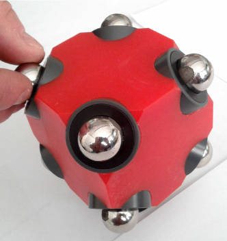
Figure 1: The “magnetic cube”. Eight spherical magnets are located at the corners of a cube and can rotate freely in their positions fixed by the cube.

A particularly simple design for a classroom demonstration of a magnetic coupling is presented in Fig. 1.schonke2015a It contains eight spherical magnets located at the corners of a cube, which is done here by providing eight holes in the corners of a Makrolon® cube. Because the spheres easily rotate inside the holes (additional ball bearings are helpful but not crucial), they will arrange automatically and find their position in the magnetic ground state, where they attract each other. When turning one of the spheres around the diagonal axis of the cube, the other seven rotate as well, all around their freely chosen axes, namely their corresponding space diagonal. The rotation can be performed without the need to overcome a magnetically induced mechanical resistance. This technical advantage is known as cogging free in the context of magnetic motors and gears. The physical reason lies in the fact that the magnetic ground state of this eight-dipole arrangement forms a degenerate continuum with respect to dipole rotations around the space diagonal. Although this is a rather nontrivial demonstration of a cogging free magnetic clutch from a mathematical point of view,schonke2015a it has the charm that this simple apparatus can be assembled directly in the classroom (by preferably four students working together, because eight hands are needed during the assembly process). The machinery described in the present paper contains only two magnetic spheres. It is conceptually simpler and presumably more suitable for technical applications than the sevenfold magnetic clutch shown in Fig. 1, but it is mechanically costlier due to the need of additional fixed rotation axes.

The theoretical description of such gears designed with spherical magnets can be based on the concept of pure dipole-dipole interaction for two dipoles $\vec{m}_{1}$ and $\vec{m}_{2}$. The coupling of two rotating dipoles with predefined rotation axis has been discussed by Schönke.schonke2015b He proposed a family of geometrical arrangements of the two rotation axes, for which the coupling should be cogging free. One type of coupling, the so-called trivial one, is reminiscent of the well-known coupling in magnetic stirrers, while the nontrivial one is characterized by the fact that the driven sphere changes its sense of rotation when compared to the trivial one. The latter one did not yet lead to real technical application, but it seems worth mentioning that a school student recently participated in a scientific competition with a toy car making use of this drive.jugendforscht2017 In the current paper the first measurement of both couplings within a single experimental setup is presented, together with a theoretical description based on dipole-dipole interaction.

II Experimental Set-up

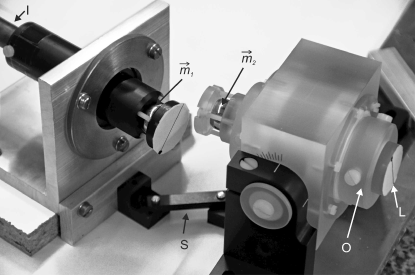
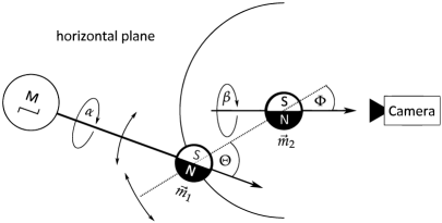
Figure 2: Top: Photograph of the experimental setup with the input shaft I, the output shaft O, the two dipoles $\vec{m}_{1}$ and $\vec{m}_{2}$, the spacer S and the line L (for further explanations, see main text). Not shown here are the motor that turns the input shaft and the camera which records the line.
Bottom: Top view schematic of the experimental setup with all parts remaining in the same horizontal plane. A computer controlled stepper motor M rotates the input shaft with the dipole $\vec{m}_{1}$ by the input dipole angle $\alpha$, thus giving rise to a rotation of the output shaft with the dipole $\vec{m}_{2}$ by the output dipole angle $\beta$. $\beta$ is detected by a CCD-camera which is also controlled by the PC. The input shaft angle $\Theta$ denotes the angle between the input shaft and the dotted line connecting the two dipoles, while the output shaft angle $\Phi$ is the respective angle for the output shaft. The center of $\vec{m}_{2}$ is fixed in space and the distance between $\vec{m}_{1}$ and $\vec{m}_{2}$ is kept constant by a spacer. The center of $\vec{m}_{1}$ together with the input shaft can be shifted on a circular arc around the center of $\vec{m}_{2}$ such, that $\Theta$ is kept constant but $\Phi$ is changed. The input shaft can be turned around the center of $\vec{m}_{1}$, thus changing $\Theta$.

A photograph of the setup is given in Fig. 2, top, while a schematic top view of the horizontal plane in which the experiments take place is shown in Fig. 2, bottom. We study the interaction of two rotating dipoles in the following geometry:volkel2016 ; borgers2016 each dipole is attached to a shaft, with the dipole moments being perpendicular to the axis of the respective shaft, and can rotate about the respective axis. Both axes always remain in the same horizontal plane. One of the shafts (the drive or input unit) is actively driven by a stepper motor, while the other shaft (the output unit) can rotate freely. The two dipoles are realized by spherical neodymium permanent magnets with diameters of $19\,$mm each. They are attached to the shafts such, that their dipole moments are perpendicular to the respective axis with a precision of about $3^{\circ}$. The comparison of the magnetic field of such a sphere with that of an ideal point dipole is given in appendix V.

Due to the strong magnets and the forces they exert on the system, the shaft bearings need special attention. We use non-magnetic and electrically non-conducting bearings. The input shaft runs in a bearing consisting of a plastic cage with glass beads, which was constructed in our in-house workshop, and is connected to the stepper motor by an $80\,$cm long brass rod. In this way, the motor and the magnets do not interfer magnetically. The output shaft runs in an industrial ceramic bearing made from zirconium oxide. In order to visualize the orientation of the dipole $\vec{m}_{2}$, a marker in form of a black line on a white background is attached to the end of the output shaft. This line is recorded by a CCD-camera.

The stepper motor and the CCD-camera are both connected to a computer, so that the input dipole angle $\alpha$ (through the stepper motor) and the output dipole angle $\beta$ (by digital image processing) are recorded and can be evaluated. The output shaft is fixed to a granite table, while the input shaft can be freely oriented on this table. A spacer is used to keep the distance between the dipoles constant during a set of experiments, while the relative orientation of the two axes can be varied.

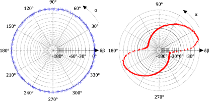
Figure 3: Phase jitter $\delta\beta$ as a function of the input dipole angle $\alpha$ for a cogging free (left; $\Theta\approx\Phi\approx 0^{\circ}$) and for a non cogging free coupling (right; $\Theta\approx-16^{\circ}$ and $\Phi\approx-61^{\circ}$).

Figure 3 shows two examples of quasi-static measurements in polar coordinates. The angular coordinate represents the input dipole angle $\alpha$, while the radial coordinate shows the phase jitter $\delta\beta$, which is the deviation of $\beta$ from the value expected for a perfectly phase-locked operation and characterizes the deviation from a cogging free motion as described in detail in the following section. The left image corresponds to $\Theta\approx\Phi\approx 0^{\circ}$, an arrangement which is realized in magnetic stirrers with no cogging between the two magnets. The circle indicates, that $\beta$ follows $\alpha$ almost perfectly, but the phase jitter plot cannot show a constant phase shift, which in this case is $180^{\circ}$. The general case, however, is different with an example shown in the right image for $\Theta\approx-16^{\circ}$ and $\Phi\approx-61^{\circ}$. Here, $\beta$ depends in a nonlinear fashion on $\alpha$. Such a motion is accompanied by non-zero cogging.

III Theoretical Background

The interaction between two point dipoles can be described following the textbook by Jackson.jackson The magnetic flux density of a dipole moment $\vec{m}_{1}$ sitting at the origin is given at a location $\vec{r}$ by

$$\vec{B}_{1}(\vec{r})=\frac{\mu_{0}}{4\pi}\,\frac{3(\vec{m}_{1}\cdot\vec{r})\vec{r}-\vec{m}_{1}\,r^{2}}{r^{5}}$$ (1)

If a second dipole $\vec{m}_{2}$ is located at $\vec{r}$, it has the potential energy $E=-\vec{m}_{2}\cdot\vec{B}_{1}(\vec{r})$. In order to model the setup described in section II, we use the coordinate system shown in Fig. 4. The centers of the dipoles, with a distance $d$ between them, and their corresponding rotation axes lie in the horizontal $x$-$y$-plane and enclose with the $x$-axis the angles $\Theta$ and $\Phi$, respectively. In order to describe the experiments unambiguously, we choose the $z$-axis upwards in the vertical direction although gravity does not play a role. The orientations of the two dipoles during their rotations are described by the angles $\alpha$ and $\beta$, respectively.

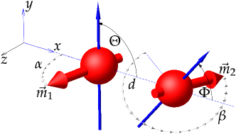
Figure 4: The coordinate system with the relevant angles. The $x$-axis points from the center of the input dipole (left red sphere) to the center of the output dipole (right red sphere), which are a distance $d$ apart. Both rotation axes (blue arrows) lie in the $x$-$y$-plane and enclose with the $x$-axis the angles $\Theta$ and $\Phi$, respectively. $\Theta$ is defined to range from $-180^{\circ}$ (negative $y$) to $+180^{\circ}$ (positive $y$), while $\Phi$ only ranges from $-90^{\circ}$ to $+90^{\circ}$, so that the output axis always points away from the input dipole. The angles $\alpha$ and $\beta$ both start in the $x$-$y$-plane and describe the orientations $\vec{m}_{1}$ and $\vec{m}_{2}$ of the dipoles, which are represented by the thick red arrows. Each dipole moment is perpendicular to its respective rotation axis.

With these definitions and following the calculations by Schönke,schonke2015b the input and output dipole moments and the position vector can be written as

$$\vec{m}_{1} = m_{1}\,\left(\begin{array}[]{c}-\cos\alpha\,\sin\Theta\\ \cos\alpha\,\cos\Theta\\ \sin\alpha\end{array}\right)\,,$$ (5)

$$\vec{m}_{2} = m_{2}\,\left(\begin{array}[]{c}-\cos\beta\,\sin\Phi\\ \cos\beta\,\cos\Phi\\ \sin\beta\end{array}\right)\,,\quad\vec{r}=d\,\left(\begin{array}[]{c}1\\ 0\\ 0\end{array}\right)\,.$$ (12)

Inserting these expressions into Eq. (1), we find for the potential energy of the output dipole $\vec{m}_{2}$ in the field of the input dipole $\vec{m}_{1}$

$$E =\frac{\mu_{0}}{4\pi}\,\frac{m_{1}\,m_{2}}{d^{3}}\cdot$$

$$\cdot\big{(}\sin\alpha\,\sin\beta+(\cos\Theta\,\cos\Phi-2\,\sin\Theta\,\sin\Phi)\,\cos\alpha\,\cos\beta\big{)}\,.$$

The system is described by seven parameters: $m_{1}$, $m_{2}$ und $d$ define the strength of the interaction, while the four angles $\Theta$, $\Phi$, $\alpha$ and $\beta$ define the type of rotation of the dipoles. For the further discussion, we rescale the energy to the dimensionless form $\tilde{E}=E/(\frac{\mu_{0}}{4\pi}\,\frac{m_{1}\,m_{2}}{d^{3}})$.

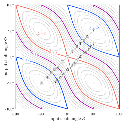
Figure 5: Contour plot of the orientation index $\Delta$ in the $\Theta$–$\Phi$-plane (see Eq. 14). The areas above $\Phi=90^{\circ}$ and below $\Phi=-90^{\circ}$ are steady continuations of the area within these borders, as $\Phi$ has been defined to range only from $-90^{\circ}$ to $+90^{\circ}$. The lines for $\Delta=1$ (red), $\Delta=0$ (violet) and $\Delta=-1$ (blue) are emphasized for better readability. The numbers from   to   in the white squares and from   to   in the white circles denote our measurement points, which will be discussed in section IV.

The orientation of the two rotation axes with respect to the line connecting the dipoles determines the value of the (shaft) orientation index $\Delta$,

$$\Delta=\cos\Theta\,\cos\Phi-2\,\sin\Theta\,\sin\Phi\,,\vspace*{-0.5ex}$$ (14)

which is constrained to the interval between $-2$ and 2 and plotted in Fig. 5. The rescaled energy can then be written as

$$\tilde{E}=\sin\alpha\,\sin\beta+\Delta\,\cos\alpha\,\cos\beta\,.$$ (15)

In our experiment, the angle $\alpha$ of the input dipole is prescribed by a stepper motor, while the output dipole can rotate freely. The output is in an equilibrium position for $\frac{\partial\tilde{E}}{\partial\beta}=\sin\alpha\,\cos\beta-\Delta\,\cos\alpha\,\sin\beta=0$. For $\alpha=\pm 90^{\circ}$ and $\beta=\pm 90^{\circ}$, this is fulfilled for any $\Delta$. These cases, where the dipoles are perpendicular to the $x$-$y$-plane, represent fix points for all configurations independent of $\Delta$ and will be discussed later. For $\alpha,\beta\neq\pm 90^{\circ}$, $\frac{\partial\tilde{E}}{\partial\beta}=0$ is equivalent to $\tan\alpha-\Delta\,\tan\beta=0$.

For $\Delta\neq 0$, the equlibrium angle $\beta_{\text{eq}}$ of the output dipole can now be given as a function of the input dipole angle $\alpha$ as

$$\beta_{\text{eq}}=\arctan\left(\frac{1}{\Delta}\,\tan\alpha\right)+\,k\cdot 180^{\circ}\,\,\text{with integer $k$}.$$ (16)

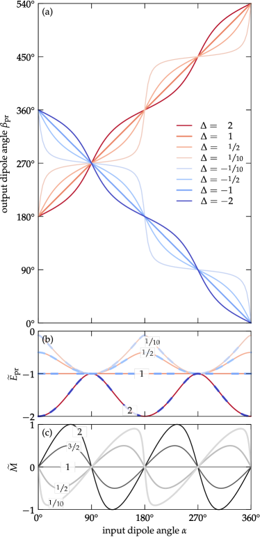
Figure 6: The preferred angle $\beta_{\text{pr}}$ (a), the equilibrium enery $\tilde{E}_{\text{pr}}$ (b), and the cogging-torque $\tilde{M}$ (c) are shown as functions of the input dipole angle $\alpha$ for various values of $\Delta$. Cogging free couplings are realized for $\Delta=\pm 1$, leading to the two straight lines with slopes $\pm 1$ in (a), to a constant $\tilde{E}_{\text{eq}}=-1$ in (b), and to $\tilde{M}=0$ in (c). The numbers at the lines in (b) and (c) are the respective values of $|\Delta|$.

The system naturally chooses $k$ such that $\beta_{\text{eq}}$ minimizes $\tilde{E}$ locally ($\frac{\partial^{2}\tilde{E}}{\partial\beta^{2}}>0$) yielding the prefered angle $\beta_{\text{pr}}$. This condition restricts $k$ to $k=\frac{3}{2}+(\left[\frac{\alpha}{180^{\circ}}\right]-\frac{1}{2})\text{sgn}\Delta$, where sgn is the signum function and the square brackets indicate convergent rounding to the nearest integer. $\left[\frac{\alpha}{180^{\circ}}\right]$ ensures the continuous extension of $\beta_{\text{pr}}$ outside the interval $[-180^{\circ};+180^{\circ}]$ and may be omitted for small $\alpha$. This energetically optimal angle is shown in Fig. 6(a) for some characteristical values of $\Delta$.

Obviously, the sign of $\Delta$ has the main influence on the behavior: For positive $\Delta$, an increasing $\alpha$ results in an increasing $\beta_{\text{pr}}$, so that the two dipoles rotate in the same direction, while a negative $\Delta$ leads to a counter-rotation. The absolute value of $\Delta$ determines the smoothness of the interaction. For $\Delta=\pm 1$, $\beta_{\text{pr}}(\alpha)$ becomes a straight line with slope $\pm 1$, so that $\beta_{\text{pr}}$ follows $\alpha$ smoothly without a phase shift. The deviation from the straight line is determined by $\Delta$ and moreover, it is the same for $\Delta$ and $1/\Delta$, but on different sides of the line. This is demonstrated by $|\Delta|=2$ and $|\Delta|=0.5$ in Fig. 6(a). The closer $\Delta$ gets to 0, the more steplike the function becomes. The lines for the different configurations cross in one of the fix points mentioned above.

Inserting $\beta_{\text{pr}}$ into Eq. (15) yields the corresponding potential energy $\tilde{E}_{\text{pr}}$ as a function of $\alpha$ (see Fig. 6b for different $\Delta$). Only the absolute value of $\Delta$ is important, so that the curves for $\Delta$ and $-\Delta$ coincide. The meaning of the straight lines in Fig. 6(a) for $\Delta=\pm 1$ becomes clear now: the potential energy is constant and thus independent of the angle of the driving dipole, so that no energy is needed to turn the second dipole: a cogging-free clutch!schonke2015b For $\Delta\neq\pm 1$ this is not the case, and the amplitude of $\tilde{E}_{\text{eq}}$ in Fig. 6(b) represents the energy needed during half a turn.

Differentiating the potential energy in Eq. (III) with respect to $\alpha$, we find the cogging-torque $M$, an important variable for the motor. The dimensionless cogging torque $\tilde{M}=\frac{\partial\tilde{E}}{\partial\alpha}$ is shown in Fig. 6(c). Again, the special meaning of the fix points is emphasized: no cogging torque is exerted on the second dipole.

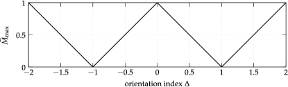
Figure 7: The torque $\tilde{M}_{\text{max}}$ that is needed to rotate the driving dipole by half a turn is shown as a function of the orientation index $\Delta$. For $\Delta=\pm 1$, this torque is zero while for any other values of $\Delta$, a finite torque is required.

In order to rotate the driving dipole by half a turn, a finite torque must be exerted which is given by the maximum $\tilde{M}_{\text{max}}$ of the respective curve. This shows a surprisingly simple dependence on $\Delta$:

$$\tilde{M}_{\text{max}}=\big{|}1-|\Delta|\big{|}$$ (17)

and is plotted in Fig. 7. Again, the special cases $\Delta=\pm 1$ are obvious, leading to vanishing torques. In the $\Delta$-landscape plot of Fig. 5, the contour lines for $\Delta=\pm 1$ are emphasized, depicting the pairs of $\Theta$ and $\Phi$ for vanishing torques. Since $\Delta(\Theta,\Phi)$ is a continuous function, there is always a line with $\Delta=0$ between those two lines. Thus, by crossing the line $\Delta=0$ through variation of $\Theta$ or $\Phi$, the sense of rotation of the output dipole with respect to the driving dipole changes.

Let us now assume that the input and output shafts are parallel, so that $\Theta=\Phi$. This situation corresponds to the black diagonal line through the center of Fig. 5. The point in the middle, $\Theta=\Phi=0$, belongs to a co-axial setup with $\Delta=1$, so that the two dipoles rotate cogging free in the same direction (see Fig. 8, left). By parallel shifting one of the two shafts, we move along the black line in Fig. 5, e.g. upwards to the right through $\Delta=0$ (maximal cogging torque), thus changing the sense of rotation, to the point with $\Delta=-1$. This point is reached for $\Theta=\Phi\approx 54.74^{\circ}$ and again corresponds to a cogging free rotation, but now with the two dipoles rotating in opposite directions (see Fig. 8, right). Thus we can shift gears by shifting the two axes.

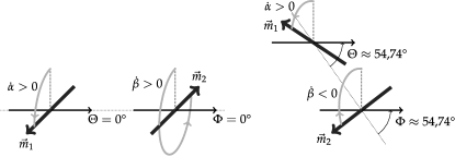
Figure 8: The two cogging free couplings for $\Theta=\Phi$. While the left part represents the trivial coupling with co-rotating dipoles like in a magnetic stirrer ($\Theta=\Phi=0$, $\Delta=1$), the right image represents the nontrivial coupling with counter-rotating dipoles ($\Theta=\Phi\approx 54.74^{\circ}$, $\Delta=-1$). The grey arrows indicate the direction of rotation of the respective dipoles.

Couplings with a finite but fixed angle between the two shafts correspond to lines in Fig. 5 which are parallel to the one just discussed. An example for $\Theta=\Phi-45^{\circ}$ is shown by the lower black line, and again we can switch from co- to counter-rotating dipoles by shifting the axes.

IV Experimental Results and Discussion

Two measurement series have been performed: In the first series, the input and output shafts are parallel ($\Phi=\Theta$), while in the second series, the two rotation axes enclose an angle of $45^{\circ}$ ($\Phi=\Theta-45^{\circ}$). The input shaft is turned with one round per minute, the slowest motion possible for the stepper motor software. After each motion we wait for the output shaft to come to a hold before measuring the output angle $\beta$. In this way, we try to realize the limit of vanishing speed of the drives. During the experiments, the internal friction in the bearings is the only load on the output shaft. In both series, we consider situations with minimal, with maximal and with intermediate cogging torques.

IV.1 Parallel rotation axes: $\Phi=\Theta$

In the simplest case of the dipole-dipole coupling, the two axes are parallel. The important parameters for this set of experiments are summarized in Tab. 1. $\Theta$ and $\Phi$ can be adjusted to approximately $1^{\circ}$, leading to an average uncertainty for $\Delta$ of about 0.04 which can rise to 0.08 near $\Delta=0$. Listed in Tab. 1 are the values $\Theta_{\text{tar}}$ and $\Phi_{\text{tar}}$, that we target in the experiment, together with the corresponding $\Delta_{\text{tar}}$.

Table 1: Parameters for parallal input and output axes ($\Phi=\Theta$) for the various measurement configurations   to  . The targeted output and input shaft angles $\Phi_{\text{tar}}$ and $\Theta_{\text{tar}}$ are adjusted manually, resulting in $\Delta_{\text{tar}}$. $\Delta_{\text{fit}}$ and $\alpha_{0}$ are results of a fit of Eq. (16) to the data points.

configuration	$\Phi_{\text{tar}}$ (∘)	$\Theta_{\text{tar}}$ (∘)	$\Delta_{\text{tar}}$	$\Delta_{\text{fit}}$	$\alpha_{0}$ (∘)
	$-90.00$	$-90.00$	$-2.000$	$-2.025$	$6.17$
	$-72.37$	$-72.37$	$-1.725$	$-1.678$	$3.60$
	$-54.74$	$-54.74$	$-1.000$	$-0.926$	$-3.59$
	$-45.00$	$-45.00$	$-0.500$	$-0.457$	$11.35$
	$-35.26$	$-35.26$	$0.001$	$0.085$	$9.74$
	$-22.50$	$-22.50$	$0.561$	$0.610$	$8.54$
	$0.00$	$0.00$	$1.000$	$0.998$	$8.10$
	$22.50$	$22.50$	$0.561$	$0.516$	$8.44$
	$35.26$	$35.26$	$-0.001$	$-0.058$	$8.99$
	$45.00$	$45.00$	$-0.500$	$-0.588$	$8.99$
	$54.74$	$54.74$	$-1.000$	$-1.133$	$8.91$
	$72.37$	$72.37$	$-1.725$	$-1.761$	$9.00$
	$90.00$	$90.00$	$-2.000$	$-2.028$	$-3.31$

The experimental $\Delta$-values are shown in Fig. 5 by the upper dashed line, which runs diagonally through the center of the graph, and where the white squares with the numbers   to   represent our measurement configurations. Numbers with the same absolute value lead to the same $\Delta$, so that similar properties are expected for the respective couplings. Our measurements are confined to values of $-90^{\circ}\leq\Theta\leq 90^{\circ}$, as a configuration with $|\Theta|>90^{\circ}$ always corresponds to one with $|\Theta|<90^{\circ}$ except for the sense of rotation.

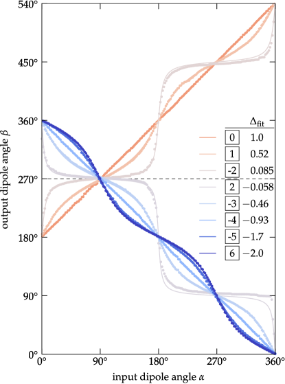
Figure 9: The measured output angle $\beta$ as a function of the input angle $\alpha$ for the measurement configurations  ,  ,  ,  ,  ,  ,   and   with the corresponding $\Delta_{\text{fit}}$ in the inset from top to bottom.

The measurements directly yield the dependence of the output dipole angle $\beta$ on the input dipole angle $\alpha$, i.e. the curves $\beta(\alpha)$ which are shown in Fig. 9. Co-rotating dipoles ($\Delta>0$) are represented by the branch that extends to the right upwards, while counter-rotating dipoles ($\Delta<0$) are represented by the branch that extends to the right downwards. We find cogging free couplings for three of the configurations: the measurements for configuration   with $\Delta=1$ and for the two configurations   (and  , not shown in Fig. 9) with $\Delta=-1$ are in good approximation linear in the $\beta(\alpha)$-graph. The coupling   shows a trivial rotational symmetry, where the two rotation axes are not only parallel but also co-axial, as shown in Fig. 8, left. The couplings for configurations   (and  ), on the other hand, are not quite as obvious. The axes are still parallel, but laterally shifted as shown in Fig. 8, right, leading to a non-trivial cogging free counter-rotation. These results are in agreement with the theory.

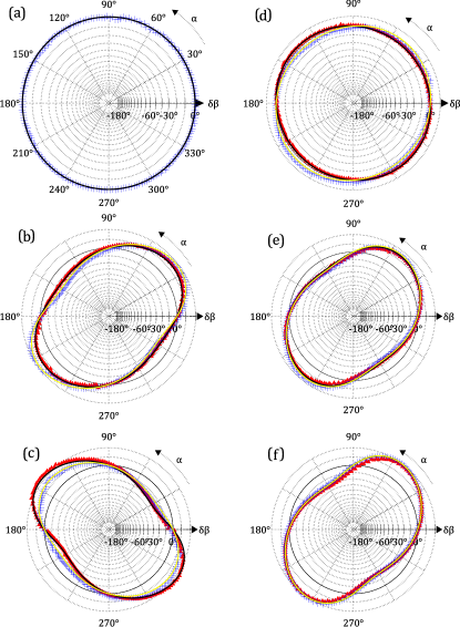
Figure 10: Phase jitter $\delta\beta$ as a function of the input dipole angle $\alpha$ for the measurements with parallel rotation axes. (a) Measurement configuration   with $\Theta\approx\Phi\approx 0^{\circ}$. (b) Configurations   with $\Theta\approx\Phi\approx-22.5^{\circ}$ and   with $\Theta\approx\Phi\approx 22.5^{\circ}$. (c) Configurations   with $\Theta\approx\Phi\approx-45^{\circ}$ and   with $\Theta\approx\Phi\approx 45^{\circ}$. (d) Configurations   with $\Theta\approx\Phi\approx-55^{\circ}$ and   with $\Theta\approx\Phi\approx 55^{\circ}$. (e) Configurations   with $\Theta\approx\Phi\approx-72^{\circ}$ and   with $\Theta\approx\Phi\approx 72^{\circ}$. (f) Configurations   with $\Theta\approx\Phi\approx-90^{\circ}$ and   with $\Theta\approx\Phi\approx 90^{\circ}$. The red triangles are for configuration with negative numbers, while the blue squares are for positive numbers. The black lines are the respective fits for negative numbers, while the yellow lines are the fits for positive numbers.

The further $\Delta$ deviates from $\pm 1$, the more the $\beta(\alpha)$-curve deviates from the linear dependence. For $\Delta$ close to 0, the dependence becomes almost steplike (measurement configurations   and  ). When $\alpha$ increases from $90^{\circ}$ to $180^{\circ}$, for most of the turn $\beta$ hardly changes and then suddenly jumps to the new equilibrium values. This corresponds to the fact that for $\Delta=0$, the coupling changes from co- to counter-rotation. For half of the cycle, $\beta$ lags extremely behind $\alpha$, while for the other half, $\beta$ is far ahead of $\alpha$.

Together with the experimental data points, fits of Eq. (16) to the data are also shown in Fig. 9. As the starting point of $\alpha$ is not perfectly known due to static friction of the shafts in the bearings and also due to uncertainties while adjusting the setup to a new $\Delta$, an offset $\alpha_{0}$ is assumed in the fits. Therefore, our free fit parameters are $\Delta$ and $\alpha_{0}$. Our measurement data are in very good agreement with the theoretical predictions with the biggest deviations for configurations with the maximal cogging torque, i.e. near $\Delta=0$. In Tab. 1, the results of the fit procedure for $\Delta_{\text{fit}}$ and $\alpha_{0}$ are also given. $\Delta_{\text{fit}}$ is always close to the value $\Delta_{\text{tar}}$ assumed in the experiment with the biggest relative deviations near $\Delta=0$.

The phase jitter is plotted in polar coordinates in Fig. 10 for the measurement configurations  ,  & ,  & ,  & ,  & , and  & . Again, the angular coordinate shows the input dipole angle $\alpha$ and the radial coordinate the phase jitter $\delta\beta$, i.e. how far the output is ahead (positive values of $\delta\beta$) or lags behind (negative values of $\delta\beta$) the input. The data for similar values of $\Delta$, which should lead to similar results, are always plotted in the same diagram together with the respective fits. The qualitative agreement ist obvious, albeit some bigger deviations can be seen for configurations  & ,  & , and  &  (see Fig. 10 b, c and d). Here, the values for the fitted $\Delta$ of the complementary data show larger differences.

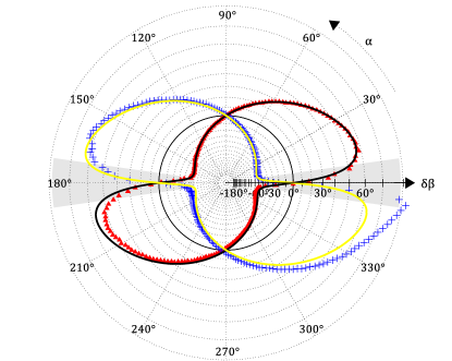
Figure 11: Phase jitter $\delta\beta$ as a function of the input dipole angle $\alpha$ for measurements near $\Delta=0$, where maximal cogging ist expected. The red triangles are for measurement configuration   ($\Theta\approx\Phi\approx-35^{\circ}$) while the blue squares are for configuration   ($\Theta\approx\Phi\approx 35^{\circ}$). The yellow and the black lines are the respective fits. Within the shaded areas, the output jumps from a maximal value of $\delta\beta$ to its minimal value.

The biggest deviation from a cogging free coupling is expected near $\Delta=0$. These results (measurement configurations  & ) are shown in Fig. 11, where the red points represent a slightly positive $\Delta$ and the blue points a slightly negative $\Delta$. It can be seen, that a slight change of $\Delta$ leads to a dramatic change in the qualitative behaviour, as the dipoles change from co-rotating to counter-rotating when crossing $\Delta=0$. Looking at the blue data points, during one half turn of the input dipole, $\delta\beta$ steadily increases until it reaches a maximal value near $\delta\beta\approx 90^{\circ}$. This is due to the fact that during this phase the output dipole hardly moves although the input dipole keeps rotating. The output lags more and more behind until the input reaches a threshold near $\alpha\approx 0^{\circ}$ or near $180^{\circ}$, when the torque transmission of the coupling is maximal and the output jumps from the maximal value of $\delta\beta$ to its minimal value (indicated by the shaded areas in Fig. 11). This jumping behavior can be attributed to the fact that the stepper motor does not turn continuously but rather has a finite step width, so that the output always has to overcome the static friction.

The theoretical model fits the data very well, leading to a value for $\Delta_{\text{fit}}$ slightly different from the experimentally assumed $\Delta_{\text{exp}}$. This can be explained by the uncertainty of the positioning of the shafts. In some cases, however, the fit does not work as well, as can be seen especially for the values of $\Delta$ near zero in Fig. 11. One reason might be the friction in the bearings and the finiteness of the motor steps. Moreover, one should not forget, that the magnets are macroscopic industrial objects and that they may not be exact point dipoles (see appendix V). Finally, it is also possible, that the dipoles are not perfectly perpendicular to the respective axis, which may explain a slightly different behaviour for complementary situations.

Table 2: Parameters for non-parallal input and output axes ($\Phi=\Theta-45^{\circ}$) for the various measurement configurations   to  . Further explanations see Tab. 1.

configuration	$\Phi_{\text{tar}}$ (∘)	$\Theta_{\text{tar}}$ (∘)	$\Delta_{\text{tar}}$	$\Delta_{\text{fit}}$	$\alpha_{0}$ (∘)
	$-90.00$	$-45.00$	$-1.414$	$-1.399$	$7.20$
	$-80.27$	$-35.27$	$-1.000$	$-1.008$	$6.79$
	$-70.47$	$-25.47$	$-0.509$	$-0.500$	$7.19$
	$-60.68$	$-15.66$	$0.001$	$0.129$	$10.10$
	$-45.00$	$0.00$	$0.707$	$0.735$	$4.32$
	$-35.26$	$9.74$	$1.000$	$1.007$	$3.93$
	$-28.82$	$16.12$	$1.109$	$1.119$	$3.75$
	$-22.50$	$22.50$	$1.146$	$1.143$	$3.97$
	$-16.12$	$28.82$	$1.109$	$1.093$	$3.94$
	$-9.74$	$35.26$	$1.000$	$0.977$	$3.59$
	$0.00$	$45.00$	$0.707$	$0.688$	$3.89$
	$15.68$	$60.65$	$0.001$	$0.132$	$5.39$
	$25.47$	$70.47$	$-0.509$	$-0.600$	$5.94$
	$35.27$	$80.27$	$-1.000$	$-1.039$	$5.39$
	$45.00$	$90.00$	$-1.414$	$-1.469$	$5.30$

IV.2 Non-parallel rotation axes: $\Phi\neq\Theta$

In a second series of experiments, we consider two rotation axes which are not parallel, but rather enclose an angle of $45^{\circ}$: $\Phi=\Theta-45^{\circ}$. The important parameters for this set of experiments are summarized in Tab. 2. The corresponding $\Delta$-values are shown in Fig. 5 by the lower dashed line, where our measurement configurations are represented by the white circles with the numbers   to  . Again, numbers with the same absolute value have the same $\Delta$.

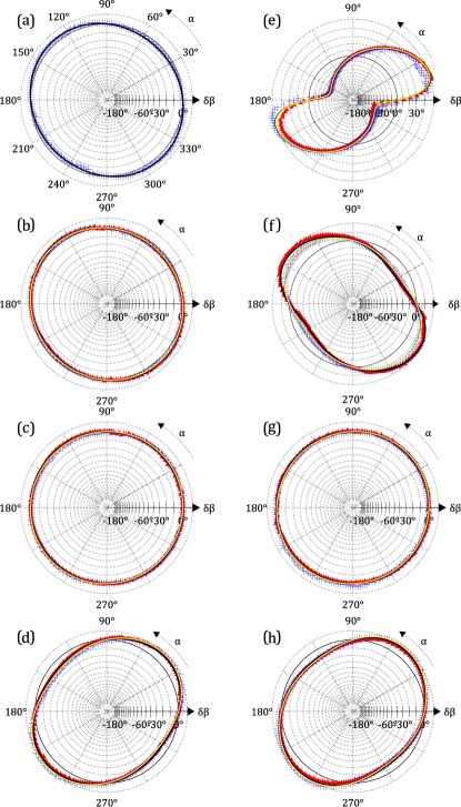
Figure 12: Phase jitter $\delta\beta$ as a function of the input dipole angle $\alpha$ for the measurements with non-parallel rotation axes. (a) Measurement configuration   with $\Theta\approx 22.5^{\circ}$, $\Phi\approx-22.5^{\circ}$. (b) Configurations   with $\Theta\approx 16^{\circ}$, $\Phi\approx-29^{\circ}$ and   with $\Theta\approx 29^{\circ}$, $\Phi\approx-16^{\circ}$. (c) Configurations   with $\Theta\approx 10^{\circ}$, $\Phi\approx-35^{\circ}$ and   with $\Theta\approx 35^{\circ}$, $\Phi\approx-10^{\circ}$. (d) Configurations   with $\Theta\approx 0^{\circ}$, $\Phi\approx-45^{\circ}$ and   with $\Theta\approx 45^{\circ}$, $\Phi\approx 0^{\circ}$. (e) Configurations   with $\Theta\approx-16^{\circ}$, $\Phi\approx-61^{\circ}$ and   with $\Theta\approx 61^{\circ}$, $\Phi\approx 16^{\circ}$. (f) Configurations   with $\Theta\approx-25^{\circ}$, $\Phi\approx-70^{\circ}$ and   with $\Theta\approx 70^{\circ}$, $\Phi\approx 25^{\circ}$. (g) Configurations   with $\Theta\approx-35^{\circ}$, $\Phi\approx-80^{\circ}$ and   with $\Theta\approx 80^{\circ}$, $\Phi\approx 35^{\circ}$. (h) Configurations   with $\Theta\approx-45^{\circ}$, $\Phi\approx-90^{\circ}$ and   with $\Theta\approx 90^{\circ}$, $\Phi\approx 45^{\circ}$. The red triangles are for configuration with negative numbers, while the blue squares are for positive numbers. The black lines are the respective fits for negative numbers, while the yellow lines are the fits for positive numbers.

The phase jitter is plotted in polar diagrams in Fig. 12 together with their fits. Again, there is a good qualitative agreement between theory and experiment as well as for configurations with the same $\Delta$. The almost perfectly circular graphs for measurement configurations  &  and  &  show a quantitative agreement with the theory (see Fig. 12c and g). Here, $|\Delta|=1$, so that cogging free couplings are expected. Both situations represent non-trivial couplings. For $\Phi\approx-10^{\circ}$ and $\Theta\approx 35^{\circ}$ (configuration  ) as well as $\Phi\approx-35^{\circ}$ and $\Theta\approx 10^{\circ}$ (configuration  ) we have $\Delta=1$, so that the dipoles are co-rotating. For $\Phi\approx 35^{\circ}$ and $\Theta\approx 80^{\circ}$ (configuration  ) and $\Phi\approx-80^{\circ}$ and $\Theta\approx-35^{\circ}$ (configuration  ), on the other hand, $\Delta=-1$, leading to counter-rotating dipoles. The other extreme of maximal cogging torque ($\Delta\approx 0$) is found for our measurement configurations   ($\Phi\approx 16^{\circ}$ and $\Theta\approx 61^{\circ}$) and   ($\Phi\approx-61^{\circ}$ and $\Theta\approx-16^{\circ}$) and are shown in Fig. 12(e).

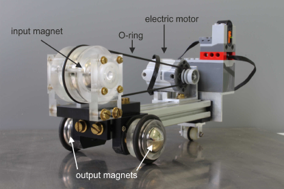
Figure 13: Toy car using a cogging free coupling with three instead of two magnets.schonke2015b ; schonke2016 The big input magnet is coupled to an electric motor by an O-ring, so that it can rotate with a constant speed. This magnet drives the two identical, but smaller output magnets which are in such positions, that the coupling is cogging free. The dipole moments of all three magnets are perpendicular to their respective rotation axes. A video of the moving car is avalable at http://www.staff.uni-bayreuth.de/~bt190039/download/AJP/car_movie.mp4.

V Conclusion and Outlook

In summary, these experiments demonstrate the crossover from trivial to non-trivial cogging free magnetic gears. The experiments can be done with commercially available spherical magnets. Their external magnetic field is in very good approximation that of an idealized point dipole. Therefore, an elementary theoretical model based on static interactions of point dipoles seems to be the adequate description of the experiments. To broaden the outlook towards technical application, we have built the toy model shown in Fig. 13, which makes use of the nontrivial coupling described in this paper. It shows the striking feature that the motor rotates in the opposite direction than the driving wheels which makes it particularly useful for classroom demonstrations. Technical applications of this kind of coupling are foreseeable for miniaturized machines where mechanical gears might be unwieldy.

*

Appendix A Dipole approximation for the spherical magnets

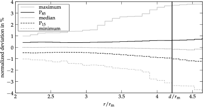
Figure 14: Characteristic percentiles for normalized deviation histograms as functions of the distance $r$ from the center of the sphere. $r_{\text{m}}$ is the radius of the sphere and the vertical line marks the distance $d$ that was realized between the two spheres in the magnetic clutch experiments presented in this paper. No residuals were found below the “minimum” and above the “maximum” line, while 50% are above and below the “median” line. The center 70% of the residuals, which indicate the standard deviation when approximating the histograms as gaussian distributions, lie between the P₁₅ and the P₈₅ lines. Therefore, the typical deviation from the ideal dipole approximation in our experiment is typically within 1%.

In order to find out how well the field of the magnets we used can be modelled by an ideal point dipole, we performed measurements of the field of the input magnet.volkel2016 For these experiments, the output shaft is replaced by a hall probe (MMT-6J02-VH with 450 Gaussmeter, Lake Shore) mounted on an $X$-$Y$ table which is oriented such that the probe scans in a plane parallel to the table on which the experiments are performed. The scanning plane is chosen as closely to the center of the input magnet as the mounting allows and lies $20\,$mm above the magnet. We sample the magnetic field at $100\times 100$ points within a rectangle of $62.5\,\text{mm}\times 75\,\text{mm}$. At each point, the component of the magnetic field parallel to the measurement plane and perpendicular to the input shaft is measured. After each scan the input shaft is rotated by $4.5^{\circ}$, thus allowing to average over all possible orientations between the dipole and the measurement plane.

An ideal dipole field is fitted to each scan and the residuals are calculated for each point. These residuals are normalized by the maximal absolute value of the magnetic field at the respective distance. The resulting normalized deviation from a point dipole approximation is then evaluated statistically yielding a histogram for each distance. Fig. 14 shows five characteristic percentiles of each histogram as functions of the distance from the center of the sphere. From this we can deduct that the normalized deviation from an ideal point dipole is approximately constant for the distances investigated here and in our experiments it is typically within 1%.

- (1) Joseph O. Hirschfelder, Charles F. Curtiss, and R. Byron Bird, Molecular Theory of Gases and Liquids, 8th edition (John Wiley & Sons Inc., 1964).
- (2) Al Adams, “Spherical Rare-Earth Magnets in Introductory Physics,” Phys. Teach. 45, 409–415 (2007).
- (3) David J. Griffiths, “Dipoles at rest,” Am. J. Phys. 60, 979–987 (1992).
- (4) Boyd F. Edwards, D. M. Riffe, Jeong-Young Ji, and William A. Booth, “Interactions between uniformly magnetized spheres,” Am. J. Phys. 85, 130–134 (2017).
- (5) J. M. Luttinger and L. Tisza, “Theory of Dipole Interaction in Crystals,” Phys. Rev. 70, 954–964 (1946).
- (6) Peter J. Belobrov, R. S. Gekht, and V. A. Ignatchenko, “Ground state in systems with dipole interaction,” Sov. Phys. JETP 57, 636–642 (1983).
- (7) N. Vandewalle and S. Dorbolo, “Magnetic ghosts and monopoles,” New J. Phys. 16, 013050 (2014).
- (8) Johannes Schönke, Tobias M. Schneider, and Ingo Rehberg, “Infinite geometric frustration in a cubic dipole cluster,” Phys. Rev. B 91, 020410-1–020410-5 (2015).
- (9) René Messina, Lara Abou Khalil, and Igor Stankovic, “Self-assembly of magnetic balls: From chains to tubes,” Phys. Rev. E 89, 011202(R) (2014).
- (10) Dominic Vella, Emmanuel du Pontavice, Cameron L. Hall, and Alain Goriely, “The magneto-elastica: from self-buckling to self-assembly,” Proc. R. Soc. A 470, 20130609 (2014).
- (11) Johannes Schönke and Eliot Fried, “Stability of vertical magnetic chains,” Proc. R. Soc. A 473 20160703 (2017).
- (12) Julien Clinton Sprott, Physics Demonstrations: A Sourcebook for Teachers of Physics, (The University of Wisconsin Press, Madison Wisconsin, 2006).
- (13) Gerald L. Pollack and Daniel R. Stump, “Two magnets oscillating in each other’s fields,” Can. J. Phys. 75, 313–324 (1997).
- (14) Arsène Chemin, Pauline Besserve, Aude Caussarieu, Nicolas Taberlet, and Nicolas Plihon, “Magnetic cannon: The physics of the Gauss rifle,” Am. J. Phys. 85, 495 (2017).
- (15) http://www.prisma.uni-mainz.de/deu/2270.php.
- (16) Mahmood H. Nagrial, “Design Optimization of Magnet Couplings Using High Energy Magnets,” Electr. Machines and Power Systems 21, 115–126 (1993).
- (17) Johannes Schönke, “Smooth Teeth: Why Multipoles Are Perfect Gears,” Phys. Rev. Appl. 4, 064007-1–064007-9 (2015).
- (18) http://www.ignaz-guenther-gymnasium.de/downloads/scichallenge_1.pdf.
- (19) John David Jackson, Classical Electrodynamics, 3rd edition (Wiley, New York, 1998).
- (20) Simeon Völkel, Rastmomentfreie kontaktlose Kupplungen aus kugelförmigen Permanentmagneten, Master thesis, University of Bayreuth (2016).
- (21) Stefan F. G. Borgers, Bestimmung des Rastmoments kontaktloser Kupplungen aus kugelförmigen Permanentmagneten, Bachelor thesis, University of Bayreuth (2016).
- (22) Johannes Schönke, Wolfgang Schöpf, and Ingo Rehberg, “Magnetkugeln — ein 10-Euro-Labor,” Physik Journal 15 4, 31–37 (2016).