The Hubble Space Telescope UV Legacy Survey of Galactic Globular Clusters - XII. The RGB Bumps of multiple stellar populations

Abstract

The Hubble Space Telescope UV Legacy Survey of Galactic Globular Clusters is providing a major breakthrough in our knowledge of Globular Clusters (GCs) and their stellar populations. Among the main results, we discovered that all the studied GCs host two main discrete groups consisting of first generation (1G) and second generation (2G) stars.

We exploit the multiwavelength photometry from this project to investigate, for the first time, the Red Giant Branch Bump (RGBB) of the two generations in a large sample of GCs. We identified, with high statistical significance, the RGBB of 1G and 2G stars in 26 GCs and found that their magnitude separation as a function of the filter wavelength follows comparable trends.

The comparison of observations to synthetic spectra reveals that the RGBB luminosity depends on the stellar chemical composition and that the 2G RGBB is consistent with stars enhanced in He and N and depleted in C and O with respect to 1G stars.

For metal-poor GCs the 1G and 2G RGBB relative luminosity in optical bands mostly depends on helium content, Y. We used the RGBB observations in F606W and F814W bands to infer the relative helium abundance of 1G and 2G stars in 18 GCs, finding an average helium enhancement $\rm\Delta Y=0.011\pm 0.002$ of 2G stars with respect to 1G stars.

This is the first determination of the average difference in helium abundance of multiple populations in a large number of clusters and provides a lower limit to the maximum internal variation of helium in GCs.

1 Introduction

The discovery of multiple stellar sequences in the photometric diagrams of Globular Clusters (GCs) in our Galaxy has raised, in the last years, new questions about the physical and dynamical processes responsible for the chemical inhomogeneities observed in different generations of stars (Bedin et al. 2004; Piotto et al. 2015, hereafter Paper I; Milone et al. 2017, hereafter Paper IX).

Indeed, several photometric and spectroscopic studies have demonstrated that the split of the characteristic evolutionary sequences in colour magnitude diagrams (CMDs) is connected to the variation, in the surface abundance of stars, of elements produced through CNO cycling and hot proton-capture processes (C-N, Na-O, Mg-Al anti-correlations) and, in turn, to helium content differences among different stellar populations (see Gratton et al. 2012; and references therein).

Various theories have been put forward so far about the nature of the primordial generation of polluters, including Asymptotic Giant Branch (AGB) stars (D’Antona et al. 2005; D’Ercole et al. 2010; D’Antona et al. 2016), fast rotating massive stars (Decressin et al. 2007), massive interacting binaries (de Mink et al. 2009) and supermassive stars (Denissenkov & Hartwick 2014), but no firm conclusion has still been achieved (see Renzini et al. 2015; hereafter Paper V, for a critical confrontation of these scenarios with the observational constraints).

Each proposed scenario envisages different yields of helium in the enriched material out of which second-generations stars are formed but we still miss information on the helium content of the different stellar populations in most GCs.

Direct measurements based on the of helium lines in the spectra of GC stars are, in fact, limited to Horizontal Branch (HB) stars with effective temperature ($T_{\rm eff}$) in the range $\sim 8,000$ – $11,500$ K (Villanova et al. 2009; Marino et al. 2014), where the cold boundary corresponds to the $T_{\rm eff}$ at which appear the first optical He i lines and the hot boundary to the $T_{\rm eff}$ at which atomic diffusion processes (gravitational settling) begin to significantly alter the surface helium abundance (Grundahl et al. 1999; Brown et al. 2016; hereafter Paper X).

An alternative method based on the observation of the chromospheric near-infrared He i transition line at $10\,830$ Å in Red Giant Branch (RGB) stars has been employed by Dupree et al. (2011) and Pasquini et al. (2011) for the clusters NGC 5139 ($\rm\omega\,Cen$) and NGC 2808, although for a few RGB stars only.

On the other hand, a multiwavelength photometric approach based on the comparison of the observed colour difference of the multiple Main Sequences (MSs) and/or RGBs with appropriate theoretical models has been applied to few GCs, namely NGC 104, NGC 288, NGC 2419, NGC 2808, NGC 5139, NGC 6352, NGC 6397, NGC 6441, NGC 6752, NGC 7078 and NGC 7089, for which the relative helium abundance of the different sub-populations was estimated (Piotto et al. 2005, 2007; Villanova et al. 2007; di Criscienzo et al. 2011; Milone et al. 2012b, c; Bellini et al. 2013; Milone et al. 2013, 2014; Nardiello et al. 2015, hereafter Paper IV).

Alongside the colour difference, an important evolutionary feature sensitive to the helium content of an old stellar population is the RGB Bump (RGBB) that, in a CMD, appears as a clump of stars along the RGB (e.g. Cassisi & Salaris 1997; and references therein). It is as well recognizable as an excess in the histogram distribution of the magnitude, or differential luminosity function (LF), of the RGB stars (Thomas 1967; Iben 1968). The RGBB is produced by the three-fold passage of the RGB stars through the same luminosity interval during their evolution.

Indeed, during the ascent of the RGB, the hydrogen-burning shell of a star steadily moves outward thereby approaching the chemical discontinuity left behind by the first dredge up. The increase in the opacity due to the larger hydrogen abundance just above the shell causes a temporary drop in the stellar luminosity that, once the shell has gone through the discontinuity, starts again to grow monotonically (Sweigart et al. 1990).

While the amplitude of the chemical discontinuity affects the RGBB lifetime, which is reflected in the size (peak height) and shape (width) of the LF excess (Bono et al. 2001; Nataf 2014), its characteristic brightness is determined by the maximum penetration of the convective envelope that, in turn, depends on parameters like age, metal abundance and helium content of the stars (Cassisi et al. 2016). For these reasons the RGBB shape and luminosity represent fundamental tools to probe the inner chemical profile of the Red Giant stars and constraints on the knowledge of the aforementioned stellar parameters in a cluster. In particular, an increase of helium makes, at fixed age and metallicity, the RGBB luminosity brighter (and the lifetime shorter). As a consequence, the RGBB location can be used to constrain the relative helium abundance of multiple populations in GCs. However, a RGBB magnitude separation caused by variations of a few percent in mass fraction of helium content, Y, in different stellar populations, is only detectable with homogeneous, high precision photometry.

An empirical investigation on the correlation between RGBB magnitude difference and helium content variation was presented in Bragaglia et al. (2010), who measured the displacement in V band of the LF peak of a combined sample of 1368 Na-poor and Na-rich Red Giants belonging to 14 GCs, corresponding to an average abundance difference in Y of $0.01\pm 0.01$ by assuming the same heavy elements distribution in the Na-poor and Na-rich stars. Similarly, Nataf et al. (2011) concluded that the gradient of the RGBB brightness and star counts with the radial distance observed in NGC 104 (47 Tuc), was consistent with the presence of a helium enriched stellar population in the cluster centre.

A previous attempt to use the RGBB magnitude difference to infer helium content variations in a GC has been done by Milone et al. (2015b; hereafter Paper III) for NGC 2808, in which two out of the five stellar populations of the cluster have a RGBB which location is compatible with a helium enrichment of $\rm Y\sim 0.03$ and $\sim 0.10$ with respect to the cluster reference population.

In this paper and in Paper III we assumed that the reference population has standard helium abundance $\rm Y=0.245+1.4\,Z$, where Z is the cluster metallicity (Pietrinferni et al. 2004). Hence, we assumed in Paper III an helium abundance of $\rm Y=0.248$ for the primordial stellar component of NGC 2808. We also verified that the resulting helium enhancement inferred for the second generation does not depend on assumed helium abundance of 1G stars.

The aim of this work, which is part of the Hubble Space Telescope (HST) UV Legacy Survey of Galactic Globular Clusters (Paper I), is to identify, for the first time, the RGBB of the distinct stellar populations of 56 GCs and constrain their differential content in helium.

Our sample includes NGC 2808, which has been analysed in Paper III using a similar method. We have excluded NGC 5139 because the multiple stellar populations in this cluster show an extreme degree of complexity (e.g. Johnson et al. 2009; Marino et al. 2011; Bellini et al. 2017) that deserves a separate analysis.

The paper is organized as follows. In Section 2 we describe the photometric catalogues, the data reduction techniques and the selection criteria of the stellar populations. The methods used to the determine the luminosity of the RGB bump for the distinct stellar populations in each GCs are described in Section 3. The comparison with theoretical models and the helium abundance estimates are illustrated in Section 4. Finally, Section 5 provides the summary and the discussion of the results.

2 Cluster database and data reduction

In the present work we have used the photometric catalogues, presented in Paper I and Paper IX, of the HST UV Legacy Survey of GCs program (G0-13297, PI G. Piotto), in UV (F275W and F336W) and optical (F438W) bands, obtained with the Ultraviolet and Visual Channel of the Wide Field Camera 3 (WFC3/UVIS) on board HST. These observations were complemented with WFC3/UVIS data collected in the same filters for GO-12605 and GO-12311 (PI G. Piotto) and from archive data that, in fact, extend the spectral coverage of the ACS/WFC optical (F606W and F814W) data of the clusters observed in the ACS Survey of GCs Treasury Program (G0-10775, PI A. Sarajedini).

Since the details on the entire dataset, exposure times and data reduction have been already provided in Paper I and Paper IX, here we briefly summarize the data reduction technique employed to obtain the final catalogues.

Each individual UVIS exposure has been corrected for poor charge-transfer efficiency according to the solution provided by Anderson & Bedin (2010). The photometric reduction has been performed with the software img2xym_wfc3uv, developed by Jay Anderson and mostly based on the program img2xym_WFC (Anderson & King 2006). The magnitude of saturated stars was recovered from saturated images with the procedure described in Anderson et al. (2008), developed from the method of Gilliland (2004), which takes into account the electrons bled into adjacent pixels. Stellar positions have been corrected for geometric distortion according to the solution of Bellini et al. (2011). Calibration to the VEGAMAG system was performed by applying the encircled energy distribution and zero points listed in the STScI website for the UVIS detector, following the recipe of Bedin et al. (2005). ACS/WFC data reduction has already been described in Anderson et al. (2008) and we refer the interested reader to this paper for details about the adopted procedures.

The catalogues have been purged from non-cluster members and photometric outliers, taking into account cluster proper motions and the quality indexes provided by the reduction software. Proper motions have been obtained by comparing the average stellar positions in two epochs (Anderson & King 2003; Piotto et al. 2012), derived from WFC3 F336W/F438W images and ACS catalogues by Anderson et al. (2008). Quality indexes provided by the software (Anderson et al. 2006, 2008) allowed to select stars measured with high-accuracy in the proper-motion selected catalogues, by adopting the procedure detailed in Milone et al. (2009). Finally the correction for differential reddening and Point Spread Function spatial variation, illustrated in Milone et al. (2012a) was applied to each catalogue.

2.1 Selection of first and second stellar populations

Spectroscopic investigation on the chemical signature of multiple populations in GCs has shown that the second stellar generations are enriched in sodium and nitrogen and depleted in carbon and oxygen, thus indicating that they formed from material exposed to some degree of CNO processing (Prantzos & Charbonnel 2006).

In this context, the F275W, F336W and F438W filters are ideal tools for the photometric identification of the distinct stellar populations because their passband encompasses the absorption wavelengths of the OH, NH, CN and CH molecules, respectively (Paper III).

This is clearly demonstrated in the $\rm m_{F336W}$ vs. $\rm C_{F275W,F336W,F438W}$ diagrams displayed in Paper I. Indeed the pseudo-colour $\rm C_{F275W,F336W,F438W}=(m_{F275W}-m_{F336W})-(m_{F336W}-m_{F438W})$, is an efficient tool to separate the multiple stellar populations along the MS, RGB and AGB.

In addition, the wide colour baseline provided by the F275W and F814W magnitudes considerably improves the sensitivity of our observations to the stellar temperature and, in turn, to helium abundance variation among multiple populations in a cluster.

To identify the two main populations we used the $\rm\Delta_{C\ F275W,F336W,F438W}$ vs. $\rm\Delta_{F275W,F814W}$ diagrams, introduced and discussed in Paper III and Paper IX. These diagrams have been referred to as chromosome maps in Paper V and we will keep using this denomination in the following. The quantities $\rm\Delta_{F275W,F814W}$ and $\rm\Delta_{C\ F275W,F336W,F438W}$ are indicative of the relative distance of a star with respect to the blue and red boundary of the RGB $\rm(m_{F275W}-m_{F814W})$ colour and the $\rm C_{F275W,F336W,F438W}$ pseudo-colour, respectively.

For example, in the upper-left panel of Figure 1 we show the chromosome map of NGC 104. A glance at the plot indicates that the star distribution is far from being homogeneous. This impression is confirmed by the corresponding stellar density diagram, shown in the lower-left panel, which displays a group of prominent clumps elongated from the upper-left to the lower-right corner and centred at $\rm(\Delta_{F275W,F814W},\Delta_{C\ F275W,F336W,F435W})\sim(-0.17,-0.32)$ and other minor clumps aligned in an almost horizontal band at $\rm\Delta_{C\ F275W,F336W,F435W}\lesssim 0.15$. In order to tag the two main stellar populations visible in this diagram, we took advantage of the selection already performed in Paper IX for all the GCs observed in the UV Legacy Survey of Galactic Globular Clusters. The plot is divided into two parts by a black dashed line. All the stars located below the line are tagged as first generation(s) (1G) and plotted over the density diagram as green dots, while the stars located above the line are tagged as secondary generation(s) (2G) and plotted as magenta dots. In the rest of the paper we will use the same colour code for 1G and 2G stars.

We note in passing that substructures are visible for each stellar group in the density diagram thus demonstrating that both 1G and 2G stars host stellar sub-populations (see for instance Milone et al. 2015a, hereafter Paper II, and Paper III and Paper IX). In this paper we are interested in the average properties of 1G and 2G stars and we focus on these two main populations only.

Paper IX has shown that the chromosome maps of a sample of GCs, including NGC 362, NGC 1261, NGC 1851, NGC 5139, NGC 5286, NGC 6388, NGC 6656, NGC 6715, NGC 6934, NGC 7089 show a split of both 1G and 2G sequences and a split SGB, which is also visible in optical CMDs. The faint and the bright SGBs are connected to the blue and red RGBs, respectively, in the $m_{\rm F336W}$ vs. $m_{\rm F336W}-m_{\rm F814W}$ CMD (see also Han et al. 2009; Marino et al. 2011, 2015). Spectroscopy reveals that red-RGB stars are enhanced in s-process elements, iron, and overall $\rm C+N+O$ abundance with respect to blue-RGB stars (Marino et al. 2009, 2012, 2015; Yong et al. 2008, 2009, 2014; Carretta et al. 2010; Johnson et al. 2015, 2017). The relative luminosity of the RGB bump of the blue and the red RGB is affected by their relative abundance of iron and $\rm C+N+O$. Since these quantities are poorly known in most of the analyzed clusters, in this paper we focus on blue-RGB stars only.

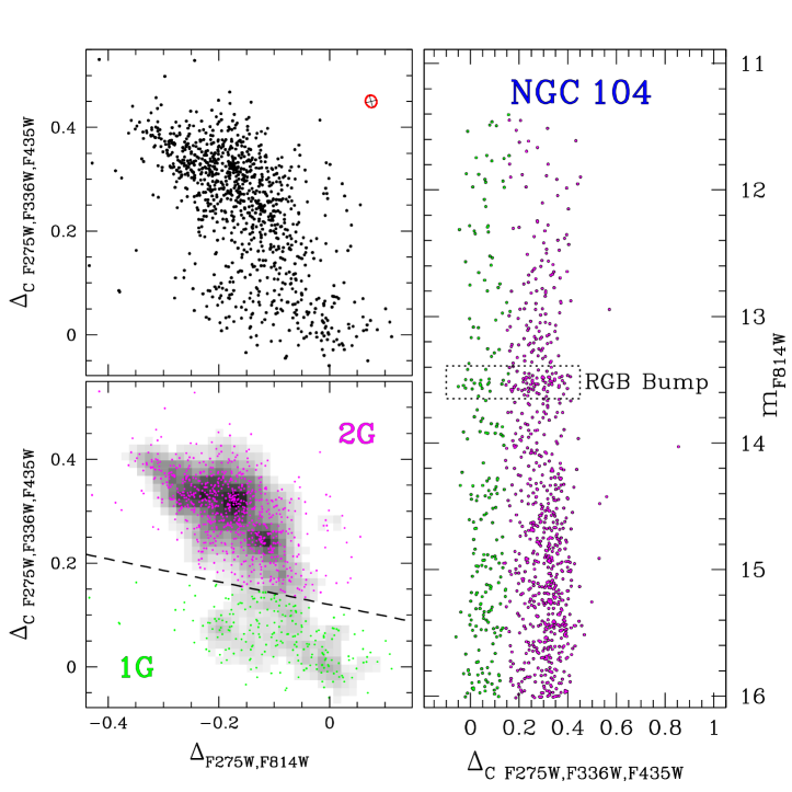
Figure 1: Upper-left panel: $\rm\Delta_{C\ F275W,F336W,F435W}$ vs. $\rm\Delta_{F275W,F814W}$ diagram (chromosome map) of the RGB stars of the GC NGC 104. The red ellipse marks the 68.27th percentile of the expected distribution of the observational errors in this diagram (see Paper IX; ). Lower-left panel: stellar density diagram relative to the chromosome map. The black dashed line divides the first (1G) and second (2G) stellar population in the chromosome map. 1G and 2G stars have been plotted over the density diagram as green and magenta dots, respectively. Right panel: $\rm m_{F814W}$ vs. $\rm\Delta_{C\ F275W,F336W,F435W}$ diagram of the cluster RGB. The dotted box indicates the approximate position of the 1G and 2G RGB Bump stars.

In the right panel of the figure we plotted the $\rm m_{F814W}$ vs. $\rm\Delta_{C\ F275W,F336W,F435W}$ diagram of the RGB stars of the cluster. We also highlighted, with a black box, the approximate location of the 1G and 2G RGBBs. In the next two sections we will describe in detail the method used to determine the RGBB luminosity and infer the average difference in helium abundance between the 1G and 2G in each cluster.

3 Determination of the RGB bumps luminosity

In this section we describe the method to estimate the magnitude difference between the RGBB of 1G and 2G stars in all the studied GCs. As an example, we illustrate in Figure 2 the procedure, in the F814W band, for the GC NGC 104.

The $\rm m_{F814W}$ vs. $\rm\Delta_{F275W,F814W}$ diagram of a portion of the cluster RGB is shown in the left panel of Figure 2. The location of the 1G and 2G RGBB is indicated by the green and the magenta bold point, respectively. For the sake of comparison, the same stars as well as the two bumps are plotted in the $\rm m_{F814W}$ vs. $\rm\Delta_{F336W,F435W}$ diagram, displayed in the middle panel, where the quantity $\rm\Delta_{F336W,F435W}$ is the analogous of $\rm\Delta_{F275W,F814W}$ but in the $\rm m_{F814W}$ vs. $\rm(m_{F336W}-m_{F435W})$ diagram.

To determine the position of the RGBB of each population we first defined a magnitude bin $w=0.1$ mag, and then built the LF of the 1G and 2G stars over a range of 0.8 mag centred on the approximate location of their RGBB, as shown in the right panel of Figure 2. Both the LFs were obtained by adopting the method of the naive estimator of Silverman (1986). In a nutshell, we divided the analysed magnitude range into a regular grid of ${\rm m}_{\rm F814W}^{i}$ points $w/10$ mag apart and, for each point, we counted the number of stars in the interval ${\rm m}_{\rm F814W}^{i}-w/2<{\rm m_{F814W}}<{\rm m}_{\rm F814W}^{i}+w/2$.

To determine the RGBB luminosity, $\rm m_{F814W,bump}$, of both the 1G and 2G stars we constructed, for each LF, a kernel density estimator by using a Gaussian kernel function with variance equal to $4/25\,w^{2}$.

The resulting kernel density estimates of the 1G and 2G stars are plotted, respectively, as green and magenta solid lines in the right panel of Figure 2. The magnitude corresponding to the maximum of each function has been taken as our best estimate of the bump luminosity for that population in the F814W band.

The error associated with each $\rm m_{F814W,bump}$ estimate was computed by carrying out 1,000 bootstrapping tests on random sampling with replacement of the RGB stars in the selected magnitude interval. The 68.27th percentile of the distribution of the bootstrapped $\rm m_{F814W,bump}$ measurements was considered the standard error of the RGBB magnitude estimate. The vertical error bar associated to the green and magenta bold points in the left and middle diagram represents, respectively, the 1G and 2G $\rm m_{F814W,bump}$ uncertainty for the cluster NGC 104.

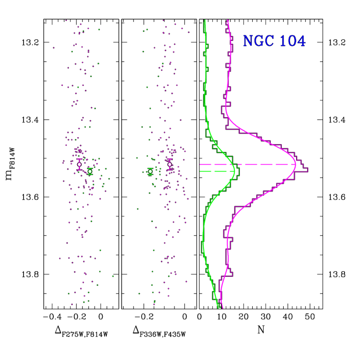
Figure 2: Left and middle panel: $\rm m_{F814W}$ vs. $\rm\Delta_{F275W,F814W}$ (left) and $\rm m_{F814W}$ vs. $\rm\Delta_{F336W,F435W}$ (right) diagram of the RGB of the GC NGC 104, approximately centred on the 1G and 2G RGBBs, marked by the green and magenta open circles, respectively. Right panel: F814W LF of the 1G (green histogram) and 2G (magenta histogram) stars displayed in the left and middle panel. The continuous line superimposed on each LF represents the corresponding kernel density estimate, which maximum indicates the RGB Bump magnitude. The uncertainty associated to the bump magnitude is plotted as a vertical error bar for the green and magenta open circles in the left and middle panels.

We applied the above procedure to derive the RGBB magnitude and the corresponding uncertainty also in the F275W, F336W, F438W and F606W bands.

Figure 3 shows the magnitude difference between the RGBB of the 2G and 1G of NGC 104, $\rm\Delta m_{X}^{(2G,1G)}$, as a function of the central wavelength of the filter X, with X = F275W, F336W, F435W, F606W, F814W. The grey dots indicate the observed difference and the corresponding error bars have been obtained by adding in quadrature the error of the 1G and 2G RGBB magnitude. We find that $\rm\Delta m_{X}^{(2G,1G)}$ is negative in the F275W, F435W, F606W and F814W bands but positive in the F336W band.

This outcome derives from the combination of the adopted filters and the chemical properties of the two different cluster populations. Indeed, the F275W and F435W (or F438W for WFC3/UVIS) filter passband encompasses, respectively, OH bands and CN and CH bands, while the F336W NH bands. Since 1G stars are carbon- and oxygen-rich and nitrogen-poor, they appear brighter than 2G stars in the F336W band and fainter in the F275W and F435W bands. Conversely 2G stars, formed by CNO-processed material, are carbon- and oxygen-poor and nitrogen-rich, therefore appearing fainter than 1G stars in F336W band and brighter in the F275W and F435W (F438W) bands (Paper I). The optical F606W and F814W filters are instead mostly sensitive to the stellar $T_{\rm eff}$, thus indicating that 2G stars are on average hotter than 1G stars, possibly due to their enhanced helium content (Milone et al. 2012b).

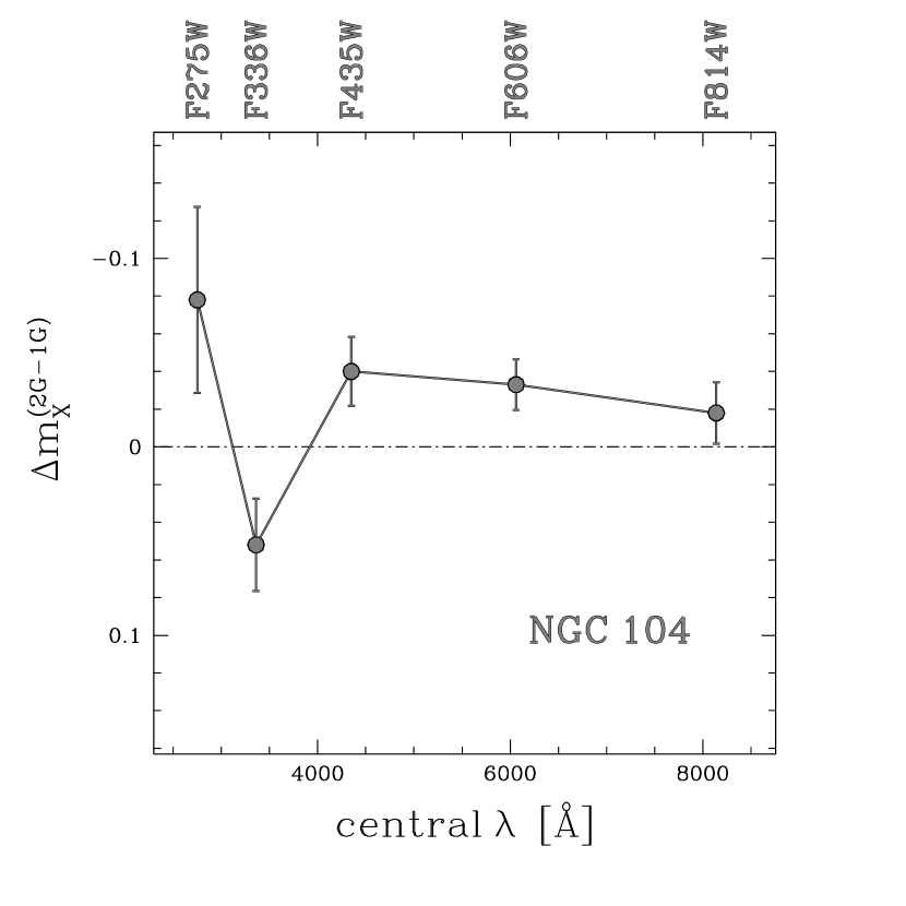
Figure 3: Magnitude difference between the 2G and 1G RGB bump of NGC 104 vs. central wavelength of the F275W, F336W, F435W, F606W, F814W filters.

3.1 Statistical significance of the RGB Bumps

The statistical significance of the RGBB detection is inferred by comparing the observations with a sample of 10,000 simulated $\rm m_{F814W}$ vs. $\rm\Delta_{F275W,F814W}$ diagrams. This method, similar to that used in Paper III, is described in the following and illustrated, for the GC NGC 104, in Figure 4. In panel (a) of Figure 4 we show the $\rm m_{F814W}$ vs. $\rm\Delta_{F275W,F814W}$ diagram of the two stellar populations of the cluster while in panel (b) we show corresponding LFs. The red and blue dot-dashed lines plotted over the LFs are the lines of best fit of the 1G and 2G LFs, respectively. Since the computation of the best-fit line of a RGB LF could be affected by the RGBB overdensity, we decided to exclude, for each LF, all the points within 0.15 mag from the corresponding RGBB. The excluded portions of the 1G and 2G LFs have been coloured green and magenta, respectively. For simplicity, in the following we indicate the corresponding magnitude interval as RGBB segment, while the difference between the area of each LF and the area below the corresponding best-fit line, in the RGBB segment, as $\rm dA_{obs}$. The fact that $\rm dA_{obs}$ is greater than zero can be either an intrinsic feature of the LF itself due to the RGBB or can be an artefact due to the photometric errors and the small number of analysed stars.

To discriminate between these two possibilities, we applied the following method to the 1G and 2G stars separately. For each stellar population we simulated 10,000 $\rm m_{F814W}$ vs. $\rm\Delta_{F275W,F814W}$ diagrams, each composed of 5,000 artificial stars. By construction, the LF of each simulated diagram has the same input slope of the observed LF best-fit line. Hence a sub-sample with the same number of stars as in the observed diagram was randomly extracted from the simulated stars. For each extracted sample of stars, we derived the LF_i and its slope by following the same prescriptions used for the observations. Then, we calculated the difference ${\rm dA}_{i,\rm sim}$ between the area of the LF in the RGBB segment and the area below the corresponding best-fit line. If ${\rm dA}_{i,\rm sim}$ were systematically smaller than $\rm dA_{obs}$, then the observed stellar overdensity would be likely due to the presence of a RGBB. In the opposite case, the observed stellar overdensity would be likely associated to a fluctuation of the LF due to the small number of analysed stars. The statistical significance is thus defined as the percentage of times on the total number of simulations in which the relation ${\rm dA}_{i,\rm sim}<\rm dA_{obs}$ is satisfied. An example of simulated diagram is provided in panel (c) of Figure 4, while the corresponding LF is shown in panel (d).

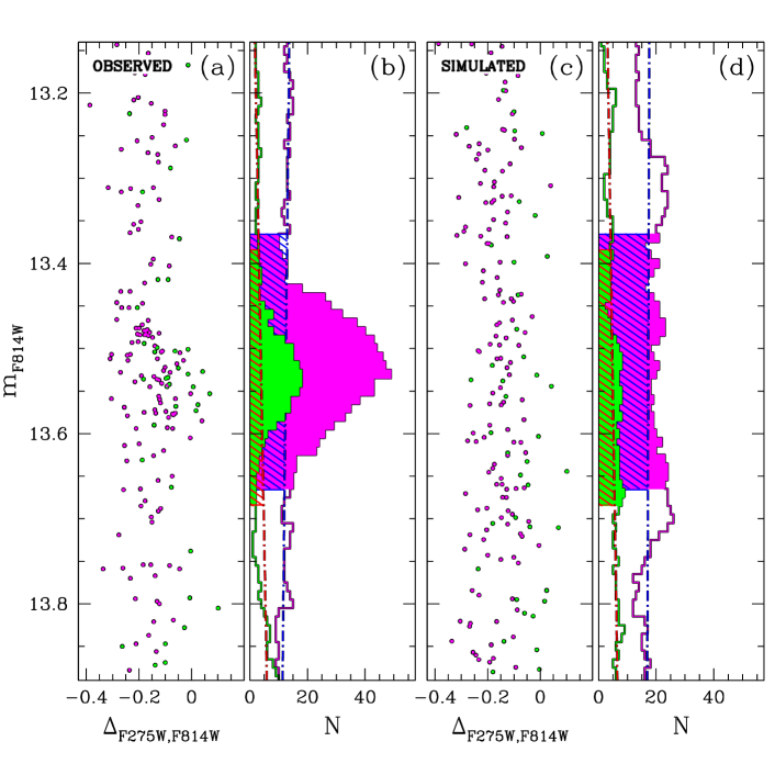
Figure 4: Estimate of the significance of the observed RGB Bump for the two stellar populations in NGC 104. In panel (a) is shown the $\rm m_{F814W}$ vs. $\rm\Delta_{F275W,F814W}$ diagram of the 1G (green) and 2G (magenta) RGB stars of the cluster while the relative LFs are plotted in panel (b). An example of simulated $\rm m_{F814W}$ vs. $\rm\Delta_{F275W,F814W}$ diagram is shown in panel (c), whereas the corresponding 1G and 2G synthetic LFs are plotted in panel (d). In panel (b) and (d), the red and blue dot-dashed lines represent, respectively, the best-fit lines of the 1G and 2G LF. The shadowed portions of each histogram correspond to the RGBB segments (see text for details).

In the case of NGC 104 we find that the RGBB is significant at the 99.6% level for the 1G stars and 100% for the 2G stars, thus demonstrating that the observed stellar overdensities observed along the two main RGBs of this cluster are due to the presence of the corresponding RGBBs.

4 Characterization of the RGB bumps

The procedure described in the previous section for NGC 104 has been applied to all the 56 GCs analyzed in this work, for which we derived the 1G and 2G RGBB magnitude and the corresponding error in all the filters as well as the 1G and 2G RGBB statistical significance in the F606W and F814W bands. For each GC, the LF was obtained by adopting $w=0.1$ mag if at least 40 stars in either the 1G or 2G sample were present in the selected 0.8 mag interval centered around the approximate location of the cluster 1G and 2G RGBBs, in the F814W band; if not $w=0.2$ mag was adopted. In both cases a grid step of $w/10$ mag was used.

Because of the poor statistics we decided to exclude from further analysis the 19 clusters with less than 15 stars in both the 1G and 2G sample in the selected F814W magnitude range, namely NGC 288, NGC 2298, NGC 3201, NGC 4590, NGC 5053, NGC 5466, NGC 5897, NGC 6101, NGC 6121, NGC 6144, NGC 6218, NGC 6366, NGC 6397, NGC 6535, NGC 6717, NGC 6779, NGC 6809, NGC 6838 and NGC 7099. Indeed, for these clusters it is not possible to unambiguously identify the presence of the 1G or 2G or both RGBBs.

In twelve clusters, namely NGC 1261, NGC 5024, NGC 5286, NGC 5904, NGC 6254, NGC 6341, NGC 6496, NGC 6541, NGC 6584, NGC 6637, NGC 6656 and NGC 7089, the significance of the RGBB of at least one population is smaller than 90% in the F814W band. Therefore, because of the low significance of their RGBB, we decided to exclude from the following analysis all the previous clusters except NGC 5904 and NGC 6637, both with a 1G RGBB significance marginally below the adopted 90% threshold. Finally, we excluded NGC 2808 because the RGBB of the multiple populations in this cluster was already analysed in Paper III.

Table 1 gives the list of the 26 clusters with 1G and 2G RGBB-detection significance $\gtrsim 90\%$, for which we indicate the magnitude difference between the 2G and 1G RGBB, $\rm\Delta m_{X}^{(2G,1G)}$, in all the bands.

Table 1: List of the 26 selected GCs with 1G and 2G RGB-Bump-detection significance $\gtrsim 90\%$. The columns 2–6 give the observed difference between the RGB Bump magnitude of the 2G and 1G stars in the F275W, F336W, F438W, F606W, F814W filter, respectively. Columns 7–8 and 9–10 give the statistical significance of the 1G–2G RGB Bumps in the F606W and F814W band, respectively.

	$\rm\Delta m_{X}^{(2G,1G)}$ (mag)										Significance (%)
Cluster	F275W		F336W		F438W		F606W		F814W		F606W		F814W
											1G	2G	1G	2G
NGC 104*	-0.078$\,\pm\,$	0.049	0.052$\,\pm\,$	0.025	-0.040$\,\pm\,$	0.018	-0.033$\,\pm\,$	0.013	-0.018$\,\pm\,$	0.016	99.0	100.0	99.6	100.0
NGC 362	-0.079$\,\pm\,$	0.016	0.044$\,\pm\,$	0.026	-0.023$\,\pm\,$	0.018	-0.023$\,\pm\,$	0.013	-0.024$\,\pm\,$	0.012	94.7	100.0	94.0	100.0
NGC 1851	-0.080$\,\pm\,$	0.022	0.033$\,\pm\,$	0.015	-0.039$\,\pm\,$	0.029	-0.029$\,\pm\,$	0.025	-0.020$\,\pm\,$	0.021	99.9	99.8	99.9	99.8
NGC 4833	-0.056$\,\pm\,$	0.057	0.123$\,\pm\,$	0.037	0.038$\,\pm\,$	0.040	0.022$\,\pm\,$	0.051	0.017$\,\pm\,$	0.056	96.0	95.8	91.6	96.6
NGC 5272	-0.081$\,\pm\,$	0.048	-0.044$\,\pm\,$	0.019	-0.065$\,\pm\,$	0.042	-0.053$\,\pm\,$	0.015	-0.047$\,\pm\,$	0.019	95.9	99.6	95.5	99.5
NGC 5904	-0.109$\,\pm\,$	0.031	0.135$\,\pm\,$	0.043	-0.023$\,\pm\,$	0.026	-0.002$\,\pm\,$	0.035	-0.003$\,\pm\,$	0.031	90.5	100.0	88.1	100.0
NGC 5927	-0.114$\,\pm\,$	0.054	0.020$\,\pm\,$	0.024	-0.037$\,\pm\,$	0.075	-0.123$\,\pm\,$	0.041	-0.121$\,\pm\,$	0.020	100.0	99.8	100.0	99.8
NGC 5986	-0.022$\,\pm\,$	0.016	0.113$\,\pm\,$	0.037	-0.010$\,\pm\,$	0.025	-0.001$\,\pm\,$	0.023	-0.009$\,\pm\,$	0.026	99.5	100.0	99.2	99.9
NGC 6093	-0.162$\,\pm\,$	0.034	0.012$\,\pm\,$	0.022	-0.080$\,\pm\,$	0.025	-0.029$\,\pm\,$	0.027	-0.053$\,\pm\,$	0.022	99.8	92.2	99.9	90.6
NGC 6171	-0.095$\,\pm\,$	0.049	0.028$\,\pm\,$	0.053	-0.122$\,\pm\,$	0.054	-0.096$\,\pm\,$	0.048	-0.086$\,\pm\,$	0.045	92.9	99.5	94.7	99.7
NGC 6205	-0.130$\,\pm\,$	0.037	0.006$\,\pm\,$	0.030	-0.081$\,\pm\,$	0.024	-0.078$\,\pm\,$	0.021	-0.082$\,\pm\,$	0.019	97.9	99.9	99.0	99.9
NGC 6304	-0.160$\,\pm\,$	0.061	0.009$\,\pm\,$	0.056	-0.069$\,\pm\,$	0.024	-0.027$\,\pm\,$	0.022	-0.010$\,\pm\,$	0.026	97.3	99.0	97.0	99.6
NGC 6352	-0.168$\,\pm\,$	0.042	-0.025$\,\pm\,$	0.030	-0.131$\,\pm\,$	0.025	-0.121$\,\pm\,$	0.031	-0.108$\,\pm\,$	0.032	99.5	99.1	99.6	98.9
NGC 6362	-0.042$\,\pm\,$	0.041	0.108$\,\pm\,$	0.034	0.027$\,\pm\,$	0.042	0.029$\,\pm\,$	0.042	0.049$\,\pm\,$	0.042	100.0	94.3	100.0	96.2
NGC 6388	0.017$\,\pm\,$	0.052	0.016$\,\pm\,$	0.019	-0.094$\,\pm\,$	0.045	-0.154$\,\pm\,$	0.062	-0.066$\,\pm\,$	0.071	91.1	100.0	94.5	100.0
NGC 6441	-0.235$\,\pm\,$	0.034	-0.011$\,\pm\,$	0.037	-0.040$\,\pm\,$	0.025	-0.038$\,\pm\,$	0.023	-0.014$\,\pm\,$	0.032	100.0	100.0	100.0	100.0
NGC 6624	-0.207$\,\pm\,$	0.041	0.023$\,\pm\,$	0.027	-0.063$\,\pm\,$	0.049	-0.068$\,\pm\,$	0.025	-0.058$\,\pm\,$	0.022	98.7	100.0	98.6	100.0
NGC 6637	-0.092$\,\pm\,$	0.022	0.111$\,\pm\,$	0.054	-0.044$\,\pm\,$	0.074	-0.022$\,\pm\,$	0.037	0.001$\,\pm\,$	0.037	83.0	100.0	89.8	100.0
NGC 6652	-0.144$\,\pm\,$	0.025	0.031$\,\pm\,$	0.025	-0.064$\,\pm\,$	0.046	-0.056$\,\pm\,$	0.036	-0.051$\,\pm\,$	0.031	99.2	99.6	99.2	99.8
NGC 6681	-0.046$\,\pm\,$	0.035	0.076$\,\pm\,$	0.027	-0.016$\,\pm\,$	0.036	-0.002$\,\pm\,$	0.038	-0.007$\,\pm\,$	0.043	99.1	93.6	99.2	93.6
NGC 6715	-0.037$\,\pm\,$	0.111	0.051$\,\pm\,$	0.066	-0.023$\,\pm\,$	0.060	-0.048$\,\pm\,$	0.027	-0.042$\,\pm\,$	0.034	99.1	99.2	98.9	99.5
NGC 6723	0.008$\,\pm\,$	0.024	0.121$\,\pm\,$	0.018	0.005$\,\pm\,$	0.016	-0.021$\,\pm\,$	0.025	-0.004$\,\pm\,$	0.022	98.2	98.7	97.8	98.6
NGC 6752*	-0.112$\,\pm\,$	0.016	0.030$\,\pm\,$	0.019	-0.043$\,\pm\,$	0.021	-0.066$\,\pm\,$	0.022	-0.072$\,\pm\,$	0.022	99.5	99.9	99.9	100.0
NGC 6934	-0.134$\,\pm\,$	0.028	0.044$\,\pm\,$	0.024	-0.072$\,\pm\,$	0.035	-0.055$\,\pm\,$	0.038	-0.054$\,\pm\,$	0.036	97.4	99.8	98.1	99.8
NGC 6981	-0.108$\,\pm\,$	0.026	0.063$\,\pm\,$	0.035	-0.037$\,\pm\,$	0.037	-0.038$\,\pm\,$	0.032	-0.030$\,\pm\,$	0.038	97.2	99.8	95.5	99.5
NGC 7078	-0.081$\,\pm\,$	0.016	0.067$\,\pm\,$	0.068	-0.100$\,\pm\,$	0.021	-0.086$\,\pm\,$	0.025	-0.095$\,\pm\,$	0.020	87.8	98.5	90.7	98.8

• The GCs NGC 104 and NGC 6752 have not been observed in the F438W filter but in the similar passband filter F435W (see Paper I; ).

Figure 5 is similar to Figure 3 and shows the magnitude difference between the RGBB of the 2G and 1G stars of all the GCs in Table 1 (except NGC 104) as a function of the central wavelength of the filter X.

A look at the plot reveals that all the GCs show comparable trends in the $\rm\Delta m_{X}^{(2G,1G)}$ vs. central $\lambda$ diagram. In all bands but F336W the 2G RGBB is brighter than the 1G RGBB, in close analogy with what we observe for NGC 104. NGC 4833 and NGC 6362 are possible exceptions because the 2G RGBB is fainter than the 1G RGBB in the three optical bands. The F438W, F606W, and F814W magnitude differences between the two main RGBBs of all the clusters are very similar to each other and are smaller than $\sim 0.1$ mag.

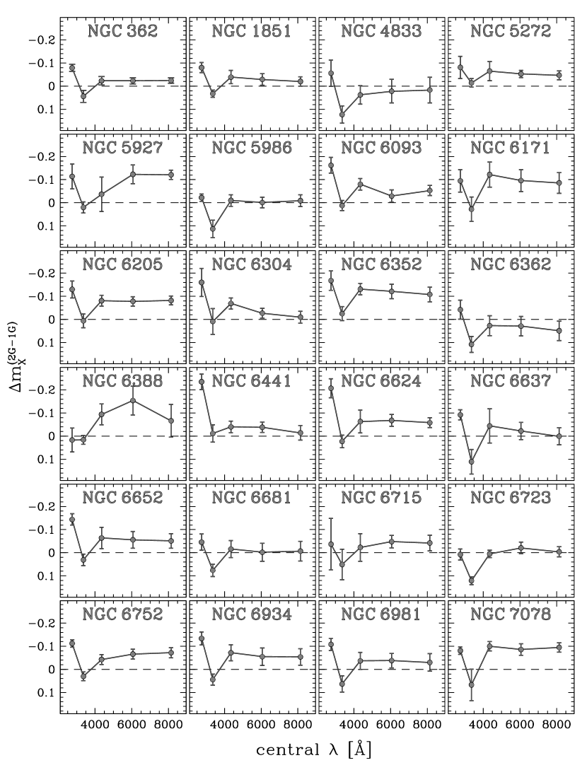
Figure 5: As in Figure 3, for all the clusters other than NGC 104, with a significance value $\geq 90\%$ in the F814W band.

4.1 The effects of C, N, and O on the RGB Bump luminosity

To investigate the physical reasons responsible for the observed magnitude difference between the RGBB of 2G and 1G stars we compared the $\rm\Delta m_{X}^{(2G,1G)}$ values with the magnitude of RGBB stars derived from synthetic spectra with appropriate chemical composition. To do this, we extended to the RGBB the procedure used in our previous papers to characterize the multiple populations along the MS and RGB. The main steps of our analysis are illustrated in Figure 6 for an RGBB star with $\rm[Fe/H]=-0.75$ (appropriate for NGC 104).

First, we determined the $T_{\rm eff}$ and gravity ($\log{g}$) corresponding to the RGBB by using isochrones from the Bag of Stellar Tracks and Isochrones (BaSTI) database  (Pietrinferni et al. 2004, 2006, 2009) with $\rm[Fe/H]=-0.75$ and age of 12.5 Gyr.

Then, we simulated two synthetic spectra with these atmospheric parameters but different C, N, O abundances that resemble the chemical composition of 1G and 2G stars inferred from high-resolution spectroscopy. Specifically, we assumed for the 1G spectrum [C/Fe]$=0.0$, [N/Fe]$=0.1$, and [O/Fe]$=0.3$, while for the comparison spectrum we used [C/Fe]$=-0.3$, [N/Fe]$=0.9$, [O/Fe]$=0.0$. These values are close to the average C, N abundances of the 1G and 2G RGB stars in NGC 104 obtained by Marino et al. (2016) and to the average O abundance derived by Carretta et al. (2009) for bright RGB stars. We assumed that these spectra have primordial helium content (Y=0.256).

To investigate the effect of helium variation on the luminosity of the RGBB, we simulated a third spectrum with the same C, N, and O abundance as 2G stars but with an higher helium content $\rm(Y=0.33)$. The corresponding atmospheric parameters are derived from BaSTI isochrones.

The ATLAS12 and SYNTHE codes (Castelli & Kurucz 2004; Kurucz 2005; Sbordone et al. 2007) are used to generate the synthetic spectra in the wavelength interval between 2,000 and 10,000 Å. In the upper panel of Figure 6 is shown the comparison between the spectra of the 1G (red) and the 2G (blue) star with primordial helium content and the 2G star with $\rm Y=0.33$ (cyan). The corresponding flux ratios are plotted in the middle panel as a function of $\lambda$. For the sake of completeness we show in the bottom panel the normalized transmission curves of the HST filters used in this work.

The flux of each spectrum has been convolved with the transmission curve of the WFC3/UVIS F275W, F336W and F438W filters and with the ACS/WFC F606W and F814W filters, to derive the corresponding synthetic magnitudes and the $\rm\Delta m_{X,CNO}^{(2G,1G)}$ values. The results are shown in the inset of the upper panel of Figure 6 where we plot the derived values of $\rm\Delta m_{X,CNO}^{(2G,1G)}$ for X = F275W, F336W, F438W, F606W and F814W.

From the comparison of the 2G and 1G spectra with primordial helium, we found that C, N, and O variations strongly affect the F275W and F336W magnitudes mostly through the OH and NH molecular bands and result in large magnitude differences between the 2G and the 1G spectrum. Carbon and nitrogen are also responsible for significant flux variation in the wavelength region covered by the F438W filter due to the absorption of CN bands. The effects of C, N, and O are less pronounced in the optical bands where the magnitude difference between the two spectra is $\lesssim 0.01$.

In contrast, the comparison between the helium-rich and primordial helium $\rm(Y=0.256)$ 2G star spectra shows that helium enhancement mostly affects the bolometric luminosity of the star, resulting in a magnitude difference of $\sim 0.07$ mag in the F606W and F814W bands.

The fact that optical magnitudes are poorly affected by C, N, O variations but are sensitive to helium, demonstrates that the magnitude difference between 2G and 1G stars in optical bands provide a strong constraint of their relative helium content.

To investigate the effect of light-element variations in the spectra of clusters with different metallicity, in Figure 7 we extended the analysis to the RGB stars of five 12.5 Gyr-old GCs with $\rm[Fe/H]=-2.5$, $-2.0$, $-1.5$, $-1.0$, $-0.5$. In all the cases we assumed for the two synthetic spectra the C, N, and O proportions used to derive the spectra plotted in Figure 6. The flux ratios of the spectra with the chemical composition of 2G stars to those with the chemical composition of 1G stars are plotted in the left panels while the right panels show the corresponding $\rm\Delta m_{X,CNO}^{(2G,1G)}$ values obtained for the five HST filters used in this paper.

In the left panels we observe that the strength of the molecular absorption bands increases with metallicity. This trend is reflected, in the right panels, in the variation of the $\rm\Delta m_{X,CNO}^{(2G,1G)}$, mostly visible in the F275W and F336W bands, as discussed above. Indeed, the F275W magnitude difference between the two spectra, that has a value of about $-0.01$ mag at $\rm[Fe/H]=-2.5$, becomes smaller than $-0.2$ mag at $\rm[Fe/H]=-0.5$, while the F336W magnitude difference steadily increases from $\sim 0.04$ mag at $\rm[Fe/H]=-2.5$ up to $\sim 0.1$ mag for $\rm[Fe/H]\sim-1.0$ and then flattens to $\sim 0.01$ towards $\rm[Fe/H]=-0.5$.

In contrast, the magnitude differences due to C, N, and O variations are typically small in the F438W, F606W and F814W filters. In particular, $\rm\Delta m_{F606W,CNO}^{(2G,1G)}$ and $\rm\Delta m_{F814W,CNO}^{(2G,1G)}$ are consistent with zero in metal-poor RGBB stars and their absolute values are significantly smaller than 0.01 mag for $\rm[Fe/H]\lesssim-0.8$. Despite being significantly affected by the strong CH bands, the F438W magnitude difference between the two spectra is quite small and is slightly larger than 0.01 mag only for $-2.2\lesssim\rm[Fe/H]\lesssim-1.2$.

A visual inspection at Figs. 3 and 5 reveals that several clusters, including metal-poor GCs, exhibit large $\rm\Delta m_{X}^{(2G,1G)}$ values in contrast with what we expect from light-element differences alone between 2G and 1G stars.

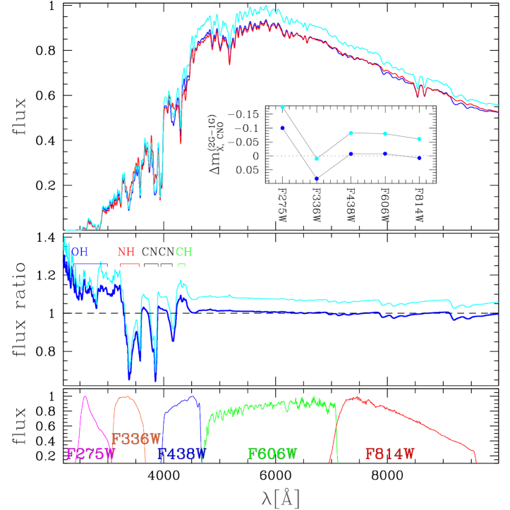
Figure 6: Comparison of 1G and 2G synthetic spectra. The red spectrum plotted in the upper panel has the same chemical composition and stellar parameters as a 1G RGB Bump star with $\rm[Fe/H]=-0.75$ and age$=12.5$ Gyr. The blue and the cyan spectra have the same metallicity and age as the red spectrum but the C, N, and O content of 2G stars. The cyan spectrum corresponds to a RGB Bump star enhanced in helium by $\rm\Delta Y=0.074$ with respect to the other two spectra, which have $\rm Y=0.256$. The ratio of the fluxes of the cyan and blue synthetic spectrum with respect to the red one are plotted in the middle panel as a function of the wavelength, while the transmission curves of the ACS/WFC and WFC3/UVIS filters used in this paper are shown in the lower panel. The inset in the upper panel shows the magnitude difference between the blue and cyan 2G spectra and the 1G synthetic spectrum in the five HST bands used in this paper. See text for details.

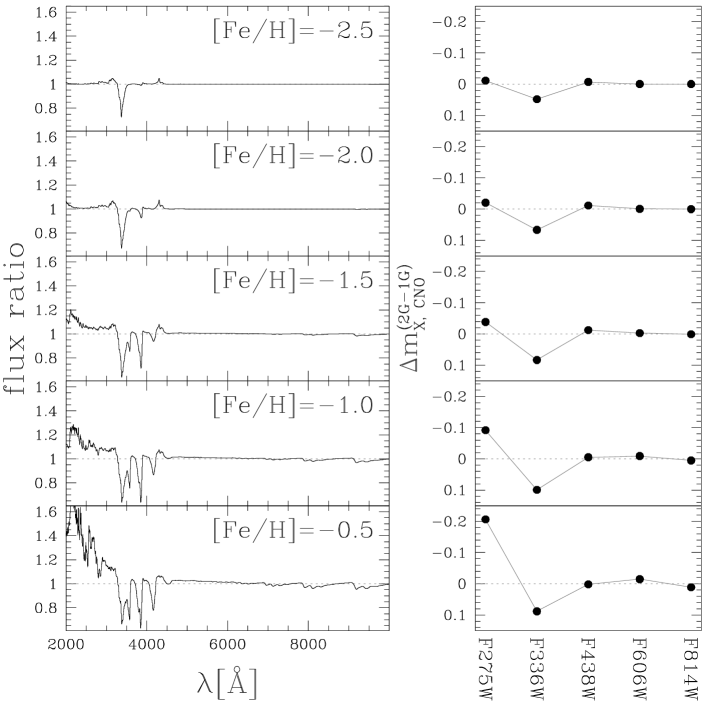
Figure 7: Flux ratio of 2G to 1G reference spectra for RGBB stars with different metallicity (left panels). The corresponding magnitude difference is plotted in the right panels for the five filters used in this paper.

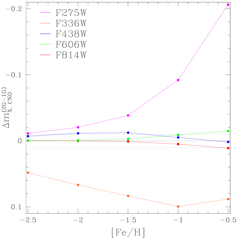
Figure 8: Magnitude difference between the comparison and the reference spectra of RGBB stars as a function of the metallicity. The five filters analysed in this paper are represented with different colours as quoted in the figure. The horizontal dotted lines are located at $\rm\Delta m_{X,CNO}^{(2G,1G)}=+/-\,0.01$.

4.2 The relative helium abundance of 1G and 2G stars

The analysis of the synthetic spectra demonstrates that C, N, and O variations alone are not able to reproduce the long-wavelength (F438W, F606W and F814W) differences between 1G and 2G stars. As a consequence, the observed magnitude of the RGBBs must also depend on the helium abundance of 1G and 2G stars and can be expressed as:

$$\rm\Delta m_{X}^{(2G,1G)}=\Delta m_{X,CNO}^{(2G,1G)}+\Delta m_{X,He}^{(2G,1G)}$$ (1)

where the last two terms of this relation indicate the contribute of the C, N, O and helium variations, respectively. In this section, we infer the helium difference between 2G and 1G stars in each cluster by comparing the observed RGBB magnitude separation with the quantities $\rm\Delta m_{X,CNO}^{(2G,1G)}$ and $\rm\Delta m_{X,He}^{(2G,1G)}$ predicted by theoretical models with appropriate chemical composition.

The quantity $\rm\Delta m_{X,CNO}^{(2G,1G)}$ has been derived for each cluster by using the procedure described in Section 4.1. As the relative C and N abundance of 1G and 2G stars is not available for most of the analysed GCs, modelling their effect on the RGBB luminosity is actually one of the main challenges of our analysis. For simplicity, we assumed for all the GCs the abundance of C, N, and O inferred from high-resolution spectroscopy of stars in NGC 104 by Carretta et al. (2009) and Marino et al. (2016). Because of this approximation, to minimize the uncertainty on the helium determination, we limited our analysis to those filters and clusters where the contribution of the C, N, and O on the RGBB luminosity is negligible, namely F606W and F814W. Indeed, in these two filters, C, N, and O variations produce RGBB luminosity differences of less than 0.01 mag for metallicities lower than $\rm[Fe/H]\sim-1.0$. Therefore, the following analysis has been performed only in the F606W and F814W bands and for the GCs with $\rm[Fe/H]\lesssim-1.0$. NGC 104, for which we have accurate C, N, O abundances from spectroscopy, is the only metal-rich cluster included in the analysis.

The F438W magnitude seems also poorly affected by the adopted C, N, and O variations. However, due to the presence of strong CN and CH bands, we prefer to not infer the helium abundance from this filter.

To estimate the quantity $\rm\Delta m_{X,He}^{(2G,1G)}$ that best matches the observations, and derive the relative helium abundance between 2G and 1G stars, we used the models of the BaSTI database.

For each cluster we calculated a grid of alpha-enhanced isochrones ([$\alpha$/Fe]$\ =0.4$): a reference isochrone with standard helium content, $\rm Y\approx 0.25$, and a set of helium-enhanced isochrones that, for helium abundances not available in the original grid, have been computed for interpolation among the available grid points. Metallicity and age values were taken respectively from Harris (1996; 2010 ed.) and Dotter et al. (2010).

To determine the helium difference between 2G and 1G stars from F814W stellar magnitudes we first generated a grid of synthetic CMDs for the RGB stars. Specifically, we simulated a CMD corresponding to the reference isochrone and 100 CMDs derived from isochrones enhanced in helium by $\rm\Delta Y$ with respect to the standard value. For each helium-enhanced isochrone, $i$, we assumed ${\rm\Delta Y}_{i}$ ranging from 0.000 to 0.100 in steps of 0.001.

Each synthetic CMD was derived by using 200,000 artificial stars (Anderson et al. 2008), to account for the observational errors in colour and magnitude. Moreover, we assumed for the LF of the reference and of each helium-rich synthetic CMD, $i$, the same slope of the corresponding observed LF.

We determined the RGBB magnitude for each couple of synthetic CMDs, by using the same procedure described in Section 3 for real stars. Then, we estimated the corresponding magnitude difference, ${\rm\Delta m}_{i\ \rm F814W,He}^{\rm(2G,1G)}$, and assumed as the best estimate of the helium difference between 2G and 1G stars the value of ${\rm\Delta Y}_{i}$ that provides: ${\rm\Delta m}_{i\ \rm F814W,He}^{\rm(2G,1G)}=\rm\Delta m_{F814W}^{(2G,1G)}-\Delta m_{X,CNO}^{(2G,1G)}$. We applied the same method to infer the helium abundance from the F606W band.

For example, the procedure for the estimate of the $\rm\Delta Y$ between the 2G and 1G stars of NGC 104 in the F814W band is displayed in Figure 9. The left panel shows the $\rm m_{F814W}$ vs. $\rm m_{F606W}-m_{F814W}$ CMD centred on the approximate location of the RGBB of the two adopted models: the red points indicate the reference isochrone, with $\rm Y=0.256$ while the blue ones the He-enhanced isochrone. The latter has a helium content of $\rm Y=0.268$, corresponding to our best estimate of the helium abundance of the 2G stars of NGC 104 in the F814W band, and has been obtained by linearly interpolating the BaSTI models with $\rm Y=0.256$ and $\rm Y=0.300$. Both the isochrones have an age of 12.75 Gyr and a metallicity of $\rm[Fe/H]=-0.72$. Since the two models almost attain the same colour, for the sake of clarity we added $-0.15$ mag to the colour of the He-enhanced isochrone.

The central panel displays the Hess diagram of the synthetic RGBs relative to the $\rm Y=0.256$ and $\rm Y=0.268$ models. The RGBB is indicated by the overdensity visible in each sequence, plotted with the same colour code of the corresponding isochrone.

Both the LFs have been normalized to the peak value of the corresponding kernel density estimate, plotted as a solid curve with the same colour code of the relative model, and the magnitude difference between the peaks of the two curves, ${\rm\Delta m}_{i\ \rm F814W,He}$ has also been reported. In the case of NGC 104, the magnitude difference due to the C, N, and O variations is $\rm\Delta m_{X,CNO}^{(2G,1G)}=0.008$ and the observed magnitude difference is $\rm\Delta m_{F814W}^{(2G,1G)}=-0.018$. Hence the adopted value of $\rm Y=0.268$, which corresponds to ${\rm\Delta m}_{i\ \rm F814W,He}^{\rm(2G,1G)}=-0.026$, satisfies equation 1 and represents the best estimate for the $\rm\Delta Y_{F814W}$.

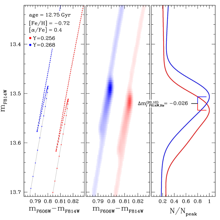
Figure 9: Procedure to estimate the helium abundance difference, $\rm\Delta Y$, between the 1G and 2G stars of NGC 104 in the F814W band. Left panel: $\rm m_{F814W}$ vs. $\rm m_{F606W}-m_{F814W}$ CMD of an alpha-enhanced BaSTI isochrone with He-standard ($\rm Y=0.256$, red points) and He-enhanced ($\rm Y=0.268$, blue points) content. The latter coincides with our best estimate of the helium content of the 2G stars of NGC 104 in the F814W band. Since the two models almost attain the same colour, the He-enhanced isochrone has been shifted of $-0.15$ mag along the colour axis. The adopted values of age, [Fe/H], and [$\alpha$/Fe] are also quoted in the figure. Central panel: $\rm m_{F814W}$ vs. $\rm m_{F606W}-m_{F814W}$ Hess diagram of the synthetic RGBs obtained from the $\rm Y=0.256$ and $\rm Y=0.268$ models (see text for details). Along each sequence, represented with the same colour code of the corresponding isochrone, is visible an overdensity that represents the RGB Bump. Right panel: Kernel density estimate of the synthetic LFs relative to the He-standard (red curve) and He-enhanced (blue curve) model. Each curve has been normalized to the corresponding peak value. The magnitude difference between the two peaks, ${\rm\Delta}_{i\ \rm F814W,He}^{\rm(2G,1G)}=-0.026$, has also been reported.

In Table 2 we provide, for the selected 18 clusters, the adopted metallicity and age values, the $\rm\Delta Y$ estimates in the F606W and F814W bands and their average value, with the corresponding standard error, in columns 2, 3, 4, 5, 6, respectively.

We notice that for each cluster the $\rm\Delta Y_{F606W}$ and the $\rm\Delta Y_{F814W}$ are consistent at $1\sigma$ level, with an average difference of $0.001\pm 0.003$. Therefore, we considered the weighted mean of the two values, $\rm\langle\Delta Y\rangle$, as our best estimate for the helium difference between the 2G and 1G stars in each cluster.

Table 2: List of the 18 selected GCs for which we estimated the $\rm\Delta Y$ by using BaSTI theoretical models. Column 6 gives the adopted estimate, $\rm\langle\Delta Y\rangle$, obtained as the weighted mean of the $\rm\Delta Y_{F606W}$ (column 4) and $\rm\Delta Y_{F814W}$ (column 5) values.

Cluster	[Fe/H]	age (Gyr)	$\rm\Delta Y_{F606W}$		$\rm\Delta Y_{F814W}$		$\rm\langle\Delta Y\rangle$
NGC 104	-0.72	12.75	0.009$\,\pm\,$	0.005	0.012$\,\pm\,$	0.007	0.010$\,\pm\,$	0.004
NGC 362	-1.26	11.50	0.006$\,\pm\,$	0.004	0.008$\,\pm\,$	0.004	0.007$\,\pm\,$	0.003
NGC 1851	-1.18	11.00	0.008$\,\pm\,$	0.008	0.007$\,\pm\,$	0.006	0.007$\,\pm\,$	0.005
NGC 4833	-1.85	13.00	-0.006$\,\pm\,$	0.016	-0.005$\,\pm\,$	0.018	-0.006$\,\pm\,$	0.012
NGC 5272	-1.50	12.50	0.013$\,\pm\,$	0.004	0.012$\,\pm\,$	0.005	0.013$\,\pm\,$	0.003
NGC 5904	-1.29	12.25	-0.002$\,\pm\,$	0.012	0.002$\,\pm\,$	0.010	0.000$\,\pm\,$	0.008
NGC 5986	-1.59	13.25	0.000$\,\pm\,$	0.006	0.002$\,\pm\,$	0.006	0.001$\,\pm\,$	0.004
NGC 6093	-1.75	13.50	0.007$\,\pm\,$	0.008	0.014$\,\pm\,$	0.006	0.011$\,\pm\,$	0.005
NGC 6171	-1.02	12.75	0.029$\,\pm\,$	0.016	0.031$\,\pm\,$	0.015	0.030$\,\pm\,$	0.011
NGC 6205	-1.53	13.00	0.020$\,\pm\,$	0.006	0.022$\,\pm\,$	0.005	0.021$\,\pm\,$	0.004
NGC 6362	-0.99	12.50	-0.014$\,\pm\,$	0.014	-0.015$\,\pm\,$	0.014	-0.014$\,\pm\,$	0.010
NGC 6681	-1.62	13.00	0.000$\,\pm\,$	0.009	0.002$\,\pm\,$	0.010	0.001$\,\pm\,$	0.007
NGC 6715	-1.49	13.25	0.013$\,\pm\,$	0.007	0.012$\,\pm\,$	0.009	0.013$\,\pm\,$	0.006
NGC 6723	-1.10	12.75	0.005$\,\pm\,$	0.008	0.003$\,\pm\,$	0.007	0.004$\,\pm\,$	0.005
NGC 6752	-1.54	12.50	0.017$\,\pm\,$	0.006	0.019$\,\pm\,$	0.006	0.018$\,\pm\,$	0.004
NGC 6934	-1.47	12.00	0.014$\,\pm\,$	0.011	0.016$\,\pm\,$	0.010	0.015$\,\pm\,$	0.007
NGC 6981	-1.42	12.75	0.012$\,\pm\,$	0.010	0.009$\,\pm\,$	0.011	0.011$\,\pm\,$	0.007
NGC 7078	-2.37	13.25	0.030$\,\pm\,$	0.010	0.033$\,\pm\,$	0.008	0.032$\,\pm\,$	0.006

The mean $\rm\Delta Y$ values indicate that, in all the analysed clusters, the 2G stars are helium enhanced with respect to the 1G stars by less than $\sim 0.035$ in mass fraction. Moreover in some clusters, namely NGC 4833, NGC 5986, NGC 6681, and NGC 6723, the 1G and 2G stars have the same helium abundance at $\sim 1\sigma$ level.

It is worth to notice that, for each cluster, the $\rm\langle\Delta Y\rangle$ value was derived by assuming that the 1G and 2G stars are coeval, as pointed out by Marino et al. (2012) for the GC NGC 6656 and by Paper IV for the GC NGC 6352. The typical error affecting the estimate of the relative age between the 1G and 2G is between 100 and 300 Myr. For this reason, we decided to relax the condition of coeval stellar generation and repeated the computation of the $\rm\Delta Y$ by assuming a population of 2G stars 100 Myr younger than 1G stars. This assumption has no significant impact on our estimates of $\rm\langle\Delta Y\rangle$. For example, we obtain, for the cluster NGC 104, a difference in $\rm\langle\Delta Y\rangle\lesssim 0.001$, which is negligible for our purposes. Moreover, we verified that the uncertainty on the age of GCs also does not affect significantly the $\rm\langle\Delta Y\rangle$ estimates. Again, in the case of NGC 104, an age difference of $\pm 0.75$ Gyr, which is the typical error of the age from Dotter et al. (2010), corresponds to a difference in $\rm\langle\Delta Y\rangle\lesssim 0.001$.

Figure 10 displays the histogram distribution of the $\rm\langle\Delta Y\rangle$ values for the selected GCs and NGC 2808 from Paper III . The histogram was built by using bins of $\rm\Delta Y=0.006$. The distribution clearly shows that, for the clusters in our sample, 2G stars are helium enriched with respect to the 1G stars with a mean value $\rm\langle\Delta Y\rangle=0.011\pm 0.002$, marked by the vertical solid line. The two dashed lines at $\rm\langle\Delta Y\rangle=0.001$ and $\rm\langle\Delta Y\rangle=0.021$ indicate the points at $+/-\,1\sigma$, respectively, with $\sigma=0.010$.

Figure 10: Distribution of the $\rm\langle\Delta Y\rangle$ values of the clusters listed in column 6 of Table 2 plus NGC 2808. The histogram was obtained by using bins of $\rm\langle\Delta Y\rangle=0.006$. The vertical solid line at $\rm\langle\Delta Y\rangle=0.011$ and the two dashed lines at $\rm\langle\Delta Y\rangle=0.001$ and $\rm\langle\Delta Y\rangle=0.021$ mark, respectively, the mean and the $+/-\,1\sigma$ of the distribution.

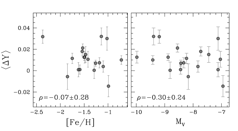
Figure 11: Plot of $\rm\langle\Delta Y\rangle$ vs. [Fe/H] (left panel) and vs. $\rm M_{V}$ (right panel) of the clusters listed in Table 2 plus NGC 2808. The values of the Spearman’s rank correlation coefficient ($\rho$) are indicated in each plot.

In Paper IX we show that the RGB width in the $\rm m_{F275W}-m_{F814W}$ colour and in the $\rm C_{F275W,F336W,F438W}$ pseudo-colour correlate with the cluster absolute luminosity and with the metallicity. Similarly, the fraction of 2G stars with respect to the total number of stars correlates with the cluster absolute luminosity thus indicating that the incidence and complexity of the multiple-population phenomenon both increase with cluster mass.

Similarly to what we have done in Paper IX, we examined the monotonic relationship between the average helium difference and both the absolute luminosity and the metallicity of the host GCs. We estimated the statistical correlation between each pair of variables by using the Spearman’s rank correlation coefficient, $\rho$, and associated to each value of $\rho$, an uncertainty $\sigma_{\rho}$, that was determined as in Milone et al. (2014) and is indicative of the robustness of the correlation coefficient. Shortly, we generated 1,000 equal-size re-samples of the original dataset by randomly sampling with replacement from the observed dataset. For each $i$-th re-sample, we have determined $\rho_{i}$ and assumed $\sigma_{\rho}$ as the 68.27th percentile of the $\rho_{i}$ measurements. As illustrated in Figure 11, we did not find any significant correlation between $\rm\langle\Delta Y\rangle$ and both [Fe/H] ($\rho=-0.07\pm 0.28$) and $\rm M_{V}$ ($\rho=-0.30\pm 0.24$). It should be noted that the lack of correlation is not in contrast with the results obtained in Paper IX because the average helium abundance differences estimated in this work represent a lower limit for the maximum helium variation in the analysed clusters.

5 Summary and conclusions

Recent studies based on multiwavelength photometry of GCs have revealed that all the analysed clusters host two discrete groups of RGB stars that correspond to the first and the second stellar generation (; ). In this paper, we used the photometric catalogues from the HST UV Legacy Survey of Galactic Globular Clusters (Paper I) and the ACS Survey of Galactic Globular Clusters Treasury Program Anderson et al. (2008), to search the RGBB of 1G and 2G stars in a large sample of 56 GCs.

We identified, for the first time, the RGBB of both 1G and 2G stars with high significance in 26 GCs by analysing the LF for the RGB stars of each population. For each cluster, we estimated the location of the two RGBBs in the F275W, F336W, F438W, F606W and F814W bands and calculated the magnitude difference between the RGBB of 2G and 1G stars, $\rm\Delta m^{(2G,1G)}_{X}$. When plotted against the central wavelength of the corresponding filter, X, the quantity $\rm\Delta m^{(2G,1G)}_{X}$ exhibits similar trends in all the analysed GCs. Specifically, the magnitude separation between the RGBBs of 2G and 1G stars is nearly the same in the F438W, F606W and F814W bands where the RGBB of 2G stars is typically brighter than that of 1G stars. The relative F336W magnitude difference between the two bumps changes significantly from one cluster to another. In some GCs, like NGC 6723, 2G stars have a RGBB fainter than that of 1G stars in the F336W band, while in other clusters, like NGC 6352 and NGC 6752, the two RGBBs have nearly the same luminosity. In contrast, the RGBB of 2G stars exhibits a F275W magnitude brighter than that of 1G stars in most GCs.

To understand the physical reasons responsible for the observed magnitude difference of the RGBB stars we computed synthetic stellar atmospheres for RGBB stars by assuming the chemical composition mixtures typical of 1G and 2G stars. We compared the $\rm\Delta m_{X}^{(2G,1G)}$ values with theoretical magnitude differences derived from the isochrones of the BaSTI databases and from synthetic spectra. We found that the luminosity of the RGBB in the F275W and F336W filters is strongly affected by the abundance of O and N respectively, through the effect of the OH and NH molecular bands on the stellar atmosphere. The F438W band is affected by strong CN and CH bands but in this case the effect on the magnitude is significantly smaller than in the UV and never exceeds 0.015 mag. Light elements also affect the stellar luminosity of RGBB stars in the F606W and F814W bands, but the corresponding magnitude variation is very small, exceeding $\sim 0.01$ mag only in GCs more metal-rich than $\rm[Fe/H]\gtrsim-1.0$.

Nevertheless, C-, N-, O-abundance variations alone are not able to reproduce the observations and some helium difference between 2G and 1G stars is needed to reproduce the observed values of $\rm\Delta m_{X}^{(2G,1G)}$. By comparing the theoretical F606W and F814W magnitudes of 1G and 2G RGBB stars derived from synthetic spectra and from isochrones, we estimated the average helium difference, $\rm\langle\Delta Y\rangle$, between 2G and 1G stars in 17 GCs with $\rm[Fe/H]\lesssim-1.0$ and in NGC 104, for which accurate C, N, and O abundances are available from high-resolution spectroscopy. This is the first determination of relative helium abundance of multiple populations in a large sample of GCs. We found that the 2G stars are more helium-rich than the 1G stars in most GCs, and that in all the GCs the average helium difference is smaller than $\rm\langle\Delta Y\rangle\sim 0.035$. On average, the 2G stars are enhanced in helium by $\rm\Delta Y=0.011\pm 0.002$ with respect to the 1G stars.

It should be noted that the estimated $\rm\langle\Delta Y\rangle$ are determined through the luminosity of the RGBB and therefore are associated to the entire stellar structure rather than to atmospheric helium abundance variations.

The findings that the stellar populations of some GCs exhibits large helium differences up to $\rm\Delta Y\sim 0.14$ (e.g. Norris 2004; D’Antona et al. 2005; Piotto et al. 2007; King et al. 2012) are not in contrast with the conclusions of this paper. Indeed, both the 2G and 1G stars of the studied GCs host sub-populations of stars with different helium and light element abundance (e.g. ; ; ). For this reason, the difference between the average helium abundance of the 2G and 1G stars is significantly smaller than the maximum helium internal variation within each GC.

The results of this paper, which are based on the luminosity of the RGBBs, further corroborate similar findings based on independent techniques and demonstrate that 2G stars are enhanced in helium, as earlier suggested by D’Antona et al. (2002) on the basis of the HB morphology of some GCs.

Most scenarios on the formation of multiple populations in GCs have suggested that 2G stars born from the material polluted from massive 1G stars. The nature of the polluters is still debated and AGB stars, fast-rotating massive stars, and supermassive stars are considered possible candidates (Paper V). In this context, several authors have estimated the helium abundance that we would expect if 2G stars formed from pure ejecta coming from a previous generation of polluting stars (e.g. Ventura & D’Antona 2009; Decressin et al. 2007; Denissenkov & Hartwick 2014).

They concluded that, if AGB or super-AGB stars are responsible for the chemical composition of 2G stars the helium content of 2G stars would never go beyond $\rm Y=0.40$, while in the case of fast-rotating massive stars we would expect that some 2G stars have helium content larger, or even much larger than 0.40 in mass fraction (e.g. Chantereau et al. 2016). However caution is necessary when using the average helium difference between 2G and 1G stars to constrain the maximum helium (and light elements) variations predicted by pollution models. Indeed, the average helium difference between 2G and 1G stars does not necessarily reflect or correlate with the maximum internal variations of the same element in GCs.

Both the average and the maximum helium abundance variations represent essential ingredients to shed light on the knowledge of the formation process of 2G stars in GCs.

References

- Anderson & King (2003) Anderson, J., & King, I. R. 2003, AJ, 126, 772
- Anderson & King (2006) Anderson, J., & King, I. R. 2006, Instrument Science Report ACS 2006-01, 34 pages
- Anderson et al. (2006) Anderson, J., Bedin, L. R., Piotto, G., Yadav, R. S., & Bellini, A. 2006, A&A, 454, 1029
- Anderson et al. (2008) Anderson, J., Sarajedini, A., Bedin, L. R., et al. 2008, AJ, 135, 2055
- Anderson & Bedin (2010) Anderson, J., & Bedin, L. R. 2010, PASP, 122, 1035
- Bedin et al. (2004) Bedin, L. R., Piotto, G., Anderson, J., et al. 2004, ApJ, 605, L125
- Bedin et al. (2005) Bedin, L. R., Cassisi, S., Castelli, F., et al. 2005, MNRAS, 357, 1038
- Bellini et al. (2011) Bellini, A., Anderson, J., & Bedin, L. R. 2011, PASP, 123, 622
- Bellini et al. (2013) Bellini, A., Piotto, G., Milone, A. P., et al. 2013, ApJ, 765, 32
- Bellini et al. (2017) Bellini, A., Anderson, J., Bedin, L. R., et al. 2017, ApJ, 842, 6
- Bono et al. (2001) Bono, G., Cassisi, S., Zoccali, M., & Piotto, G. 2001, ApJ, 546, L109
- Bragaglia et al. (2010) Bragaglia, A., Carretta, E., Gratton, R., et al. 2010, A&A, 519, A60
- Brown et al. (2016) Brown, T. M., Cassisi, S., D’Antona, F., et al. 2016, ApJ, 822, 44
- Carretta et al. (2009) Carretta, E., Bragaglia, A., Gratton, R. G., et al. 2009, A&A, 505, 117
- Carretta et al. (2010) Carretta, E., Gratton, R. G., Lucatello, S., et al. 2010, ApJ, 722, L1
- Cassisi & Salaris (1997) Cassisi, S., & Salaris, M. 1997, MNRAS, 285, 593
- Cassisi et al. (2016) Cassisi, S., Salaris, M., & Pietrinferni, A. 2016, A&A, 585, A124
- Castelli & Kurucz (2004) Castelli, F., & Kurucz, R. L. 2004, arXiv:astro-ph/0405087
- Chantereau et al. (2016) Chantereau, W., Charbonnel, C., & Meynet, G. 2016, A&A, 592, A111
- D’Antona et al. (2002) D’Antona, F., Caloi, V., Montalbán, J., Ventura, P., & Gratton, R. 2002, A&A, 395, 69
- D’Antona et al. (2005) D’Antona, F., Bellazzini, M., Caloi, V., et al. 2005, ApJ, 631, 868
- D’Antona et al. (2016) D’Antona, F., Vesperini, E., D’Ercole, A., et al. 2016, MNRAS, 458, 2122
- Decressin et al. (2007) Decressin, T., Meynet, G., Charbonnel, C., Prantzos, N., & Ekström, S. 2007, A&A, 464, 1029
- de Mink et al. (2009) de Mink, S. E., Pols, O. R., Langer, N., & Izzard, R. G. 2009, A&A, 507, L1
- Denissenkov & Hartwick (2014) Denissenkov, P. A., & Hartwick, F. D. A. 2014, MNRAS, 437, L21
- D’Ercole et al. (2010) D’Ercole, A., D’Antona, F., Ventura, P., Vesperini, E., & McMillan, S. L. W. 2010, MNRAS, 407, 854
- di Criscienzo et al. (2011) di Criscienzo, M., D’Antona, F., Milone, A. P., et al. 2011, MNRAS, 414, 3381
- Dotter et al. (2010) Dotter, A., Sarajedini, A., Anderson, J., et al. 2010, ApJ, 708, 698
- Dupree et al. (2011) Dupree, A. K., Strader, J., & Smith, G. H. 2011, ApJ, 728, 155
- Gilliland (2004) Gilliland, R. L. 2004, Instrument Science Report ACS 2004-01, 18 pages
- Gratton et al. (2012) Gratton, R. G., Carretta, E., & Bragaglia, A. 2012, A&ARv, 20, 50
- Grundahl et al. (1999) Grundahl, F., Catelan, M., Landsman, W. B., Stetson, P. B., & Andersen, M. I. 1999, ApJ, 524, 242
- Han et al. (2009) Han, S.-I., Lee, Y.-W., Joo, S.-J., et al. 2009, ApJ, 707, L190
- Harris (1996) Harris, W.E. 1996, AJ, 112, 1487
- Iben (1968) Iben, I. 1968, Nature, 220, 143
- Johnson et al. (2009) Johnson, C. I., Pilachowski, C. A., Michael Rich, R., & Fulbright, J. P. 2009, ApJ, 698, 2048
- Johnson et al. (2015) Johnson, C. I., Rich, R. M., Pilachowski, C. A., et al. 2015, AJ, 150, 63
- Johnson et al. (2017) Johnson, C. I., Caldwell, N., Rich, R. M., et al. 2017, ApJ, 836, 168
- King et al. (2012) King, I. R., Bedin, L. R., Cassisi, S., et al. 2012, AJ, 144, 5
- Kurucz (2005) Kurucz, R. L. 2005, Memorie della Societa Astronomica Italiana Supplementi, 8, 14
- Marino et al. (2009) Marino, A. F., Milone, A. P., Piotto, G., et al. 2009, A&A, 505, 1099
- Marino et al. (2011) Marino, A. F., Milone, A. P., Piotto, G., et al. 2011, ApJ, 731, 64
- Marino et al. (2012) Marino, A. F., Milone, A. P., Piotto, G., et al. 2012, ApJ, 746, 14
- Marino et al. (2014) Marino, A. F., Milone, A. P., Przybilla, N., et al. 2014, MNRAS, 437, 1609
- Marino et al. (2015) Marino, A. F., Milone, A. P., Karakas, A. I., et al. 2015, MNRAS, 450, 815
- Marino et al. (2016) Marino, A. F., Milone, A. P., Casagrande, L., et al. 2016, MNRAS, 459, 610
- Milone et al. (2009) Milone, A. P., Bedin, L. R., Piotto, G., & Anderson, J. 2009, A&A, 497, 755
- Milone et al. (2012a) Milone, A. P., Piotto, G., Bedin, L. R., et al. 2012, A&A, 537, A77
- Milone et al. (2012b) Milone, A. P., Piotto, G., Bedin, L. R., et al. 2012, ApJ, 744, 58
- Milone et al. (2012c) Milone, A. P., Marino, A. F., Cassisi, S., et al. 2012, ApJ, 754, L34
- Milone et al. (2013) Milone, A. P., Marino, A. F., Piotto, G., et al. 2013, ApJ, 767, 120
- Milone et al. (2014) Milone, A. P., Marino, A. F., Dotter, A., et al. 2014, ApJ, 785, 21
- Milone et al. (2015a) Milone, A. P., Marino, A. F., Piotto, G., et al. 2015, MNRAS, 447, 927
- Milone et al. (2015b) Milone, A. P., Marino, A. F., Piotto, G., et al. 2015, ApJ, 808, 51
- Milone et al. (2017) Milone, A. P., Piotto, G., Renzini, A., et al. 2017, MNRAS, 464, 3636
- Nardiello et al. (2015) Nardiello, D., Piotto, G., Milone, A. P., et al. 2015, MNRAS, 451, 312
- Nataf et al. (2011) Nataf, D. M., Gould, A., Pinsonneault, M. H., & Stetson, P. B. 2011, ApJ, 736, 94
- Nataf (2014) Nataf, D. M. 2014, MNRAS, 445, 3839
- Norris (2004) Norris, J. E. 2004, ApJ, 612, L25
- Pasquini et al. (2011) Pasquini, L., Mauas, P., Käufl, H. U., & Cacciari, C. 2011, A&A, 531, A35
- Pietrinferni et al. (2004) Pietrinferni, A., Cassisi, S., Salaris, M., & Castelli, F. 2004, ApJ, 612, 168
- Pietrinferni et al. (2006) Pietrinferni, A., Cassisi, S., Salaris, M., & Castelli, F. 2006, ApJ, 642, 797
- Pietrinferni et al. (2009) Pietrinferni, A., Cassisi, S., Salaris, M., Percival, S., & Ferguson, J. W. 2009, ApJ, 697, 275
- Piotto et al. (2005) Piotto, G., Villanova, S., Bedin, L. R., et al. 2005, ApJ, 621, 777
- Piotto et al. (2007) Piotto, G., Bedin, L. R., Anderson, J., et al. 2007, ApJ, 661, L53
- Piotto et al. (2012) Piotto, G., Milone, A. P., Anderson, J., et al. 2012, ApJ, 760, 39
- Piotto et al. (2015) Piotto, G., Milone, A. P., Bedin, L. R., et al. 2015, AJ, 149, 91
- Prantzos & Charbonnel (2006) Prantzos, N., & Charbonnel, C. 2006, A&A, 458, 135
- Renzini et al. (2015) Renzini, A., D’Antona, F., Cassisi, S., et al. 2015, MNRAS, 454, 4197
- Sbordone et al. (2007) Sbordone, L., Bonifacio, P., & Castelli, F. 2007, Convection in Astrophysics, 239, 71
- Silverman (1986) Silverman, B. W. 1986, Monographs on Statistics and Applied Probability, London: Chapman and Hall, 1986
- Sweigart et al. (1990) Sweigart, A. V., Greggio, L., & Renzini, A. 1990, ApJ, 364, 527
- Thomas (1967) Thomas, H.-C. 1967, Z. Astrophys., 67, 420
- Ventura & D’Antona (2009) Ventura, P., & D’Antona, F. 2009, A&A, 499, 835
- Villanova et al. (2007) Villanova, S., Piotto, G., King, I. R., et al. 2007, ApJ, 663, 296
- Villanova et al. (2009) Villanova, S., Piotto, G., & Gratton, R. G. 2009, A&A, 499, 755
- Yong et al. (2008) Yong, D., Grundahl, F., Johnson, J. A., & Asplund, M. 2008, ApJ, 684, 1159-1169
- Yong et al. (2009) Yong, D., Grundahl, F., D’Antona, F., et al. 2009, ApJ, 695, L62
- Yong et al. (2014) Yong, D., Roederer, I. U., Grundahl, F., et al. 2014, MNRAS, 441, 3396