Leptoquarks in Flavour Physics

Abstract

While the LHC has not directly observed any new particle so far, experimental results from LHCb, BELLE and BABAR point towards the violation of lepton flavour universality in $b\to s\ell^{+}\ell^{-}$ and $b\to c\ell\nu$. In this context, also the discrepancy in the anomalous magnetic moment of the muon can be interpreted as a sign of lepton flavour universality violation. Here we discuss how these hints for new physics can also be explained by introducing leptoquarks as an extension of the Standard Model. Indeed, leptoquarks are good candidates to explain the anomaly in the anomalous magnetic moment of the muon because of an $m_{t}/m_{\mu}$ enhanced contribution giving correlated effects in $Z$ boson decays which is particularly interesting in the light of future precision experiments.

1 Introduction

So far the LHC has not directly observed any particles beyond the ones in the Standard Model of particle physics (SM). While in the SM the Higgs boson couplings to fermions are the only source of lepton flavour universality violation (LFUV), in the past years several hints for additional LFUV have been accumulated. The ratios of semi-leptonic $B$ decays

$$R\left(K^{(*)}\right) ={\rm Br}\left[B\to K^{(*)}\mu^{+}\mu^{-}\right]{\bigg{/}}{\rm Br}\left[B\to K^{(*)}e^{+}e^{-}\right]\,,$$

$$R\left(D^{(*)}\right) ={\rm Br}\left[B\to D^{(*)}\tau\nu\right]{\bigg{/}}{\rm Br}\left[B\to D^{(*)}\ell\nu\right]\,,$$

$$R\bigg{(}J/\Psi\bigg{)} ={\rm Br}\bigg{[}B_{c}^{+}\to J/\Psi\tau^{+}\nu\bigg{]}{\bigg{/}}{\rm Br}\bigg{[}B_{c}\to J/\Psi\mu^{+}\nu\bigg{]}\,,$$

show sizeable deviations from the SM predictions.
Considering $b\to s\ell^{+}\ell^{-}$ transitions, $R(K)$ Aaij:2014ora and $R(K^{*})$ Aaij:2017vbb show a combined significance for LFUV at the $4\,\sigma$ level Altmannshofer:2017yso ; DAmico:2017mtc ; Hiller:2017bzc ; Geng:2017svp ; Hurth:2017hxg ; Ciuchini:2017mik . If we also take into account all other $b\to s\mu^{+}\mu^{-}$ observables, in several scenarios the global fit prefers new physics (NP) above the $5\,\sigma$ level Capdevila:2017bsm .
In $R(D^{(*)})$ BaBar Lees:2012xj , BELLE Huschle:2015rga ; Hirose:2017dxl and LHCb Aaij:2015yra ; Betti:2017xri found a significance for LFUV of about $4\,\sigma$ Amhis:2016xyh . In this context it is interesting to mention that LHCb recently measured a deviation of about $2\,\sigma$ in $R(J/\Psi)$ Aaij:2017tyk . This is consistent with the anomaly in $R(D)$ and $R(D^{*})$.
The tension in the anomalous magnetic moment of the muon $(a_{\mu})$ between measurement Bennett:2006fi and SM prediction is at the $3\,\sigma$ level Nyffeler:2016gnb ; Jegerlehner:2009ry . Also this discrepancy can be interpreted as a sign of LFUV even though the anomalous magnetic moments are already in the SM flavour non-universal: If we assume that NP coupled with the same strength to electrons and to muons, $a_{e}$ would be more sensitive for NP. Since no deviation from the SM prediction in $a_{e}$ has been observed so far, the tension in $a_{\mu}$ can be interpreted as another sign for LFUV induced by NP.
Motivated by these anomalies, we study leptoquarks (LQ) which provide a possible solution of them. Firstly we concentrate on each anomaly itself and discuss which LQ representations suit best for an explanation and consider correlated effects in other observables. Finally, we will investigate if we can explain the described anomalies simultaneously.

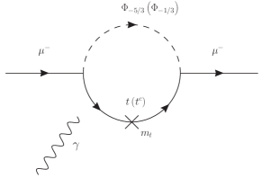
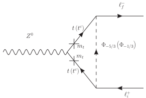
Figure 1: Feynman diagrams that contribute to $a_{\mu}$ and $Z\to\ell_{i}^{+}\ell_{f}^{-}$. The crosses on the fermion lines stand for chirality flips, involving a top mass.

2 $a_{\mu}$

In order to explain the descrepancy in $a_{\mu}$, a rather large effect of the order of the SM weak interaction contribution is required. Among the set of new particles that can give the desired effect, LQ are interesting candidates Djouadi:1989md ; Davidson:1993qk ; Couture:1995he ; Bauer:2015knc ; Das:2016vkr . Even though the LQ must be rather heavy due to LHC constraints (above 1 TeV), one can still get relevant effects in $a_{\mu}$. For some representations of LQ, the amplitude can be enhanced by a factor $m_{t}/m_{\mu}\simeq\mathcal{O}(10^{3})$ or $m_{b}/m_{\mu}\simeq\mathcal{O}(10)$ compared to the SM.
To achieve an enhancement of factor $m_{t}/m_{\mu}$, the LQ must couple to left- and right-handed top or anti-top quarks simultaneously. However, not all LQ representations have this feature. Among the 10 scalar and vector LQ representations generating lepton-quark interaction terms that are invariant under the SM gauge group Buchmuller:1986zs , only two scalars can possess this enhancement: An $\mathrm{SU}(2)$ singlet $\Phi_{1}$ and an $\mathrm{SU}(2)$ doublet $\Phi_{2}$ with quantum numbers

$$Q\left({\Phi_{1}}\right):\left({3,1,-\frac{2}{3}}\right)\,,\leavevmode\nobreak\ \leavevmode\nobreak\ \leavevmode\nobreak\ \leavevmode\nobreak\ Q\left({{\Phi_{2}}}\right):\left({\bar{3},2,-\frac{7}{3}}\right)\,.$$ (1)

These representations couple to the fermions of the SM as follows

$$\mathcal{L}_{int}= \left(\lambda_{fi}^{1R}\overline{u^{c}_{f}}\ell_{i}+\lambda_{fi}^{1L}\overline{Q^{c}_{f}}i\tau_{2}L_{i}\right)\Phi^{\dagger}_{1}\,,$$ (2)

$$\mathcal{L}_{int}= \left(\lambda_{fi}^{2RL}\overline{u_{f}}L_{i}+\lambda_{fi}^{2LR}\overline{Q_{f}}i\tau_{2}\ell_{i}\right)\Phi_{2}^{\dagger}\,.$$ (3)

$Q$ and $L$ are $\mathrm{SU}(2)$ doublets, $u$ and $\ell$ are $\mathrm{SU}(2)$ singlets and $c$ denotes charge conjugation. $f$ and $i$ are flavour indices. The Feynman diagrams involving $\Phi_{1}$ and $\Phi_{2}$ are shown left in Fig. 1.
For simplicity, we only consider couplings of top quarks to muons and set $\lambda_{32}^{1L,1R}$ and $\lambda_{32}^{2RL,2LR}$ equal to $\lambda_{\mu}^{L,R}$. Besides the contribution to $a_{\mu}$, we also obtain correlated effects in $Z\to\mu^{+}\mu^{-}$ (see the right Feynman diagram in Fig. 1), in $b\to s\nu\bar{\nu}$ (for $\Phi_{1}$) and in $b\to s\mu^{+}\mu^{-}$ (for $\Phi_{2}$). Fig. 2 shows the allowed regions in $\lambda_{\mu}^{L}$-$\lambda_{\mu}^{R}$ parameter space for a LQ with mass of $1\leavevmode\nobreak\ \mathrm{TeV}$, to respect constraints from direct searches. For $Z\to\mu^{+}\mu^{-}$ the expected bounds from GigaZ Baer:2013cma and TLEP Gomez-Ceballos:2013zzn are shown as well. Additionally, for $\Phi_{1}$ the expected BELLE II limit for $B\to K^{(*)}\nu\bar{\nu}$ is taken into account. $\Phi_{2}$ gives a $C_{9}=C_{10}$-like contribution to $b\to s\ell^{+}\ell^{-}$ which provides a slight improvement of $1\,\sigma$ in the global fit.
If we also allow for couplings of the top quark to taus or electrons, lepton flavour violating processes as $\tau\to\mu\gamma$ or $Z\to\mu e$ will be possible. A more detailed discussion can be found in Ref. ColuccioLeskow:2016dox .

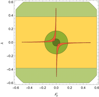
Figure 2: Allowed regions in the $\lambda^{L}_{\mu}$-$\lambda^{R}_{\mu}$ parameter space from current limits of LEP and expected future constraints of GigaZ and TLEP with $M_{LQ}=1\leavevmode\nobreak\ \mathrm{TeV}$. Left: $\mathrm{SU}(2)$ singlet $\Phi_{1}$. Right: $\mathrm{SU}(2)$ doublet $\Phi_{2}$. Note that if the expected sensitivity of TLEP was reached and no excess in the $Z\mu\bar{\mu}$-coupling was found, an explanation of the anomaly in $a_{\mu}$ would strongly be disfavoured.

3 $b\to s\ell^{+}\ell^{-}$

Dealing with $b\to s\ell^{+}\ell^{-}$ transitions, one usually works with an effective Hamiltonian of the form

$$H_{\rm eff}^{\ell_{f}\ell_{i}}=-\dfrac{4G_{F}}{\sqrt{2}}V_{tb}V_{ts}^{*}\sum\limits_{a=9,10}C_{a}^{fi}O_{a}^{fi}+C_{a}^{\prime fi}O_{a}^{\prime fi}\,,$$ (4)

$${O_{9(10)}^{fi}}=\dfrac{\alpha}{4\pi}[\bar{s}{\gamma^{\mu}}P_{L}b]\,[\bar{\ell}_{f}{\gamma_{\mu}}(\gamma_{5})\ell_{i}]\,,$$ (5)

$${O_{9(10)}^{\prime fi}}=\dfrac{\alpha}{4\pi}[\bar{s}{\gamma^{\mu}}P_{R}b]\,[\bar{\ell}_{f}{\gamma_{\mu}}(\gamma_{5})\ell_{i}]\,.$$ (6)

Then, for several scenarios with NP in $C_{9}$ only, $C_{9}=-C_{10}$ or $C_{9}=-C_{9}^{\prime}$, the global fit prefers NP above the $5\,\sigma$ level Capdevila:2017bsm .
We consider the case where NP contributes as $C_{9}=-C_{10}$. While in the muon channel the preferred value deviates from the SM prediction with a tension of $5\,\sigma$, in the case with electrons the SM contribution is sufficient to give a good fit to the data. To reach the central value, an $\mathcal{O}(10\%)$ NP effect in the muon channel is required. $b\to s\ell^{+}\ell^{-}$ is suppressed by a loop and a CKM factor because it is a flavour changing neutral current. Therefore, the effect of NP does not have to be very large to account for the data. There are several suggestions to explain the anomaly in $b\to s\mu^{+}\mu^{-}$ with LQ, see e.g. Gripaios:2014tna ; Fajfer:2015ycq ; Becirevic:2015asa ; Greljo:2015mma ; Calibbi:2015kma ; Alonso:2015sja ; Barbieri:2015yvd ; Becirevic:2016yqi ; Becirevic:2016oho ; Becirevic:2017jtw ; Aloni:2017ixa ; Chauhan:2017ndd ; Sumensari:2017mud ; Chen:2017hir .
There are three LQ representations that give a $C_{9}=-C_{10}$-like contribution to $b\to s\ell^{+}\ell^{-}$

$$\Phi_{3}:\leavevmode\nobreak\ \left(3,3,-\frac{2}{3}\right)\,,\leavevmode\nobreak\ \mathcal{L}_{int}=\lambda_{fi}^{3}\overline{Q^{c}_{f}}i\tau_{2}\left(\tau\cdot\Phi_{3}\right)^{\dagger}L_{i}\,,$$ (7)

$$V^{\mu}_{1}:\leavevmode\nobreak\ \left(\bar{3},1,-\frac{4}{3}\right)\,,\leavevmode\nobreak\ \mathcal{L}_{int}=\left(\kappa_{fi}^{1R}\overline{d_{f}}\gamma_{\mu}\ell_{i}+\kappa_{fi}^{1L}\overline{Q_{f}}\gamma_{\mu}L_{i}\right)V_{1}^{\mu\dagger}\,,$$ (8)

$$V^{\mu}_{3}:\leavevmode\nobreak\ \left(3,3,\frac{4}{3}\right)\,,\leavevmode\nobreak\ \mathcal{L}_{int}=\kappa_{fi}^{3}\overline{Q_{f}}\gamma_{\mu}\left(\tau\cdot V_{3}^{\mu}\right)L_{i}\,.$$ (9)

If we only allow for couplings to muons, these LQ will give tree-level effects in $b\to s\mu^{+}\mu^{-}$ but contribute at loop-level in other flavour observables. This is why LQ can explain the anomalies in $b\to s\mu^{+}\mu^{-}$ transitions but are not in conflict with other observables.
Including couplings to electrons, we get additional effects in $b\to se^{+}e^{-}$ as well as in the lepton flavour violating processes $\mu\to e\gamma$ and $b\to s\mu e$. We can write

$${\rm Br}\left[\mu\to e\gamma\right] \propto\left|\leavevmode\nobreak\ \chi C_{9}^{ee}+\frac{C_{9}^{\mu\mu}}{\chi}\right|^{2}\,,$$ (10)

$${\rm Br}\left[B\to K\mu e\right] \propto\left|\frac{C_{9}^{ee}}{\gamma}\right|^{2}+\left|\gamma\,C_{9}^{\mu\mu}\right|^{2}\,,$$ (11)

where $\chi=y_{32}/y_{21}$ and $\gamma=y_{21}/y_{22}$, with $y=\lambda$ for scalar LQ and $y=\kappa$ for vector LQ. Note that one can avoid an effect in $\mu\to e\gamma$ completely if $C_{9}^{\mu\mu}=-\chi^{2}C_{9}^{ee}$. For real values of $\chi$ this means that ${\rm sign}[C_{9}^{ee}]=-{\rm sign}[C_{9}^{\mu\mu}]$. In Fig. 3 you find a detailed analysis for the scalar triplet $\Phi_{3}$. For $V_{1}^{\mu}$ and $V_{3}^{\mu}$ the situation is quite similar, albeit the blue bands are more narrow. For more information see Ref. Crivellin:2017dsk .

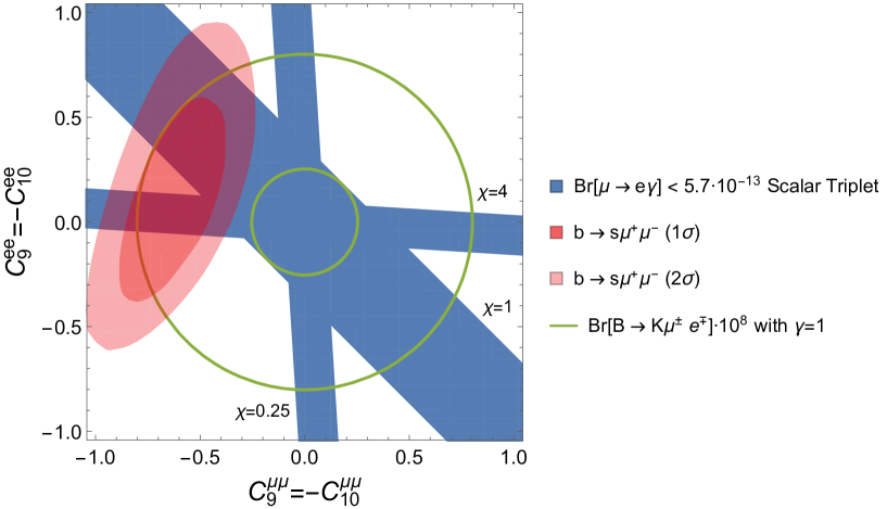
Figure 3: The darker (lighter) red region shows the global fit at $1\,\sigma$ ($2\,\sigma$) for $b\to se^{+}e^{-}$ and $b\to s\mu^{+}\mu^{-}$ transitions. In blue, the allowed region constrained by the current limit $\rm{Br}\left[\mu\to e\gamma\right]<4.2\times 10^{-13}$ TheMEG:2016wtm with $\chi=\{1/4,1,4\}$ for the scalar triplet $\Phi_{3}$ with $M_{LQ}=1\mathrm{TeV}$. The outer (inner) green contour shows the case where $\rm{Br}\left[B\to K\mu e\right]=2\times 10^{-8}(0.2\times 10^{-8})$. For real values of $\chi$ only the region with $C_{9}^{\mu\mu}<0$ and $C_{9}^{ee}>0$ seems to be compatible with experimental limits. Indeed this is also where the central value of the global fit lies. However, if in the future the global fit prefers $C_{9}^{\mu\mu}<0$ and $C_{9}^{ee}<0$, LQ with real couplings will not be able to explain $b\to s\ell^{+}\ell^{-}$ transitions without violating the constraints from $\mu\to e\gamma$.

4 $b\to c\tau\nu$

The transition $b\to c\tau\nu$ is a charged current process and is therefore generated at tree-level in the SM. Since an explanation of $R(D)$ and $R(D^{*})$ requires an $\mathcal{O}(10\%)$ effect, also the NP must contribute at tree-level. Charged Higgses Crivellin:2012ye ; Tanaka:2012nw ; Celis:2012dk ; Crivellin:2013wna ; Crivellin:2015hha , $W^{\prime}$ bosons Greljo:2015mma and LQ Alonso:2015sja ; Calibbi:2015kma ; Bauer:2015knc ; Becirevic:2016yqi ; Barbieri:2016las ; Chauhan:2017uil ; Dorsner:2017ufx ; Popov:2016fzr ; Hiller:2016kry ; Sahoo:2016pet ; Das:2016vkr ; Altmannshofer:2017poe are NP candidates. However, $B_{c}$ lifetime Akeroyd:2017mhr ; Freytsis:2015qca ; Celis:2016azn ; Li:2016vvp and $q^{2}$ distributions Celis:2016azn in combination with direct searches Faroughy:2016osc strongly disfavour charged Higgses and $W^{\prime}$ bosons.
Hence, we are left with LQ. If we want to explain the excess in $R(D)$ and $R(D^{*})$ by modifying the couplings to tau neutrinos and/or taus, we also get effects in $b\to s\tau^{+}\tau^{-}$ and $b\to s\nu\bar{\nu}$. It can be shown in a model independent way that these effects are of the order of $10^{3}$ compared to the SM Alonso:2015sja ; Capdevila:2017iqn . This is due to the fact that the processes $b\to s\tau^{+}\tau^{-}$ and $b\to s\nu\bar{\nu}$ occur at loop-level in the SM, while LQ contribute at tree-level with considerably large couplings in order to explain $R(D^{(*)})$. An $\mathcal{O}(10^{3})$ effect is in strong conflict with experimental results of $B\to K^{(*)}\nu\bar{\nu}$.
Hence, a model that explains $R(D)$ and $R(D^{*})$ must avoid a major effect in $b\to s\nu\bar{\nu}$. One possibility is the vector LQ singlet $V_{1}^{\mu}$ (see Eq. (8)). Another model was proposed in Ref. Crivellin:2017zlb , where instead of $V_{1}^{\mu}$ two scalar LQ (the $\mathrm{SU}(2)$ singlet $\Phi_{1}$ in Eq. (2) and the $\mathrm{SU}(2)$ triplet $\Phi_{3}$ in Eq. (7)) are required. If Fig. 4 we can see for which parameters we can explain $R(D^{(*)})$ without violating the limits of $b\to s\nu\bar{\nu}$.
Besides explaining $R(D^{(*)})$, it also enhances $B_{s}\to\tau^{+}\tau^{-}$ up to a factor $10^{3}$ compared to the SM and therefore lies within experimental reach. The current limit is ${\rm Br}\left[B_{s}\to\tau^{+}\tau^{-}\right]<6.8\times 10^{-3}$ Aaij:2017xqt . Fig. 5 shows the correlation of $R(D^{(*)})$ and ${\rm Br}\left[B_{s}\to\tau^{+}\tau^{-}\right]$.

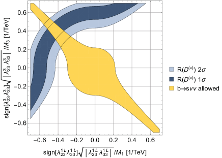
Figure 4: In lighter (darker) blue you see the $1\,\sigma$ ($2\,\sigma$) preferred region of the weighted sum of $R(D)$ and $R(D^{*})$, in yellow the allowed region of $b\to s\nu\bar{\nu}$. $M_{1(3)}$ is the mass of the LQ $\Phi_{1}$ ($\Phi_{3}$).

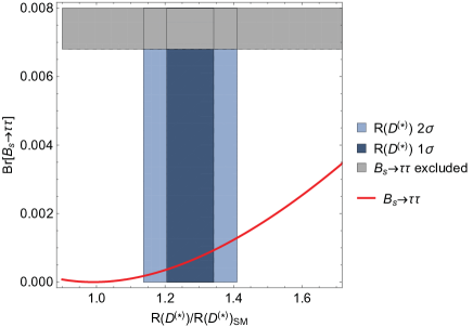
Figure 5: In blue we have the weighted sum of $R(D)$ and $R(D^{*})$ and the red line depicts the correlated prediction of ${\rm{Br}\left[B_{s}\to\tau^{+}\tau^{-}\right]}$. The grey region shows the current experimental bounds.

5 Simultaneous Explanation

We may ask if one can explain the three types of anomalies in $a_{\mu}$, $b\to s\mu^{+}\mu^{-}$ and $R(D^{(*)})$ simultaneously.
If we take the model that we proposed in Sec. 4 and insert a discrete symmetry for the couplings $\lambda_{jk}^{1L}=e^{i\pi j}\lambda_{jk}^{3}\equiv\lambda_{jk}^{L}$ the effect in $b\to s\nu\bar{\nu}$ will be cancelled exactly. If we include $b\to s\mu^{+}\mu^{-}$, $B\to D^{(*)}\mu\nu/B\to D^{(*)}e\nu$ will be affected. However, these observables remain compatible with experiments. Additionally the LFV process $\tau\to\mu\gamma$ and $b\to s\tau\mu$ appear. Both processes give constraints on our parameter space. On the left-hand side of Fig. 6 the allowed regions for $M_{LQ}=1\leavevmode\nobreak\ \mathrm{TeV}$ are shown, under the assumption that $b\to s\mu^{+}\mu^{-}$ matches the central value of the global fit. As we can see easily, the explanation of $R(D^{(*)})$ requires $\lambda^{L}_{33}/\lambda^{L}_{32}>1$. On the right-hand side of Fig. 6 we need $\lambda^{L}_{33}/\lambda^{L}_{32}<0.6$ to explain $a_{\mu}$ without getting in conflict with experimental constraints of $\tau\to\mu\gamma$. With this contradiction, we cannot explain all three anomalies simultaneously. However, if we abandon anyone of them, it is possible to explain the other two anomalies. If we abandon the assumption $\lambda_{jk}^{1L}=e^{i\pi j}\lambda_{jk}^{3}$ one can avoid the discussed constraints and explain all three anomalies.
Another good candidate is the vector LQ singlet $V_{1}^{\mu}$ because it does not affect the $b\to s\nu\bar{\nu}$ transitions but gives a $C_{9}=-C_{10}$ effect in $b\to s\ell^{+}\ell^{-}$. It can also be used to explain $R(D^{(*)})$. In $a_{\mu}$ we can obtain an $m_{b}/m_{\mu}$ contribution which is not as large as for the two scalar LQ $\Phi_{1}$ and $\Phi_{2}$ (see Sec.2), but still may be significant.
However, one faces the problem that massive vector bosons without a Higgs mechanism are not renormalizable. For $\ell^{\prime}\to\ell\gamma$ in Sec. 3 this does not cause a problem because this process is finite in unitary gauge. Recently, models containing renormalizable massive vector LQ were proposed DiLuzio:2017vat ; Calibbi:2017qbu ; Bordone:2017bld ; Barbieri:2017tuq . In Ref. Calibbi:2017qbu a Pati-Salam model in combination with vector-like fermions is phenomenologically consistent and leads to a massive vector LQ. This vector LQ has the properties of $V_{1}^{\mu}$ in Eq. (8).

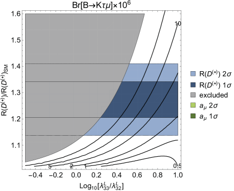
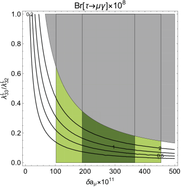
Figure 6: Left: In blue we have the weighted sum of $R(D)$ and $R(D^{*})$. The contour lines show ${\rm Br}\left[B\to K\tau\mu\right]\times 10^{6}$. Right: The anomaly in $a_{\mu}$ combined with the contour lines depicting ${\rm Br}\left[\tau\to\mu\gamma\right]\times 10^{8}$. In both plots the grey region is excluded by experiments.

6 Conclusion

In these proceedings we reviewed which LQ are good candidates to explain flavour anomalies: For the deviation in $a_{\mu}$ the scalar LQ $\Phi_{1}$ and $\Phi_{2}$ give an $m_{t}/m_{\mu}$ enhanced contribution. This is a useful feature to explain the rather large discrepancy. Considering $b\to s\ell^{+}\ell^{-}$ transitions, the three LQ representations $\Phi_{3}$, $V_{1}^{\mu}$ and $V_{3}^{\mu}$ are required by the fit, because they give $C_{9}=-C_{10}$. $R(D^{(*)})$ can be explained either by $V_{1}^{\mu}$ or, as we proposed, by a combination of a scalar LQ singlet $\Phi_{1}$ and scalar LQ triplet $\Phi_{3}$ without getting in conflict with $b\to s\nu\bar{\nu}$ observables. We also showed that this model is able to explain any two of the three anomalies ($a_{\mu}$, $b\to s\mu^{+}\mu^{-}$ and $R(D^{(*)}$) simultaneously.

Acknowledgments

D.M. thanks the organizing committee, and especially Giancarlo D’Ambrosio, for the invitation and for giving the opportunity to present his work.
D.M. is supported by an Ambizione Grant of the Swiss National Science Foundation (PZ00P2_154834).

References

- (1) R. Aaij et al. [LHCb Collaboration], Phys. Rev. Lett. 113 (2014) 151601 doi:10.1103/PhysRevLett.113.151601 [arXiv:1406.6482 [hep-ex]].
- (2) R. Aaij et al. [LHCb Collaboration], JHEP 1708 (2017) 055 doi:10.1007/JHEP08(2017)055 [arXiv:1705.05802 [hep-ex]].
- (3) W. Altmannshofer, P. Stangl and D. M. Straub, Phys. Rev. D 96 (2017) no.5, 055008 doi:10.1103/PhysRevD.96.055008 [arXiv:1704.05435 [hep-ph]].
- (4) G. D’Amico, M. Nardecchia, P. Panci, F. Sannino, A. Strumia, R. Torre and A. Urbano, JHEP 1709 (2017) 010 doi:10.1007/JHEP09(2017)010 [arXiv:1704.05438 [hep-ph]].
- (5) G. Hiller and I. Nisandzic, Phys. Rev. D 96 (2017) no.3, 035003 doi:10.1103/PhysRevD.96.035003 [arXiv:1704.05444 [hep-ph]].
- (6) L. S. Geng, B. Grinstein, S. JÃger, J. Martin Camalich, X. L. Ren and R. X. Shi, Phys. Rev. D 96 (2017) no.9, 093006 doi:10.1103/PhysRevD.96.093006 [arXiv:1704.05446 [hep-ph]].
- (7) T. Hurth, F. Mahmoudi, D. Martinez Santos and S. Neshatpour, Phys. Rev. D 96 (2017) no.9, 095034 doi:10.1103/PhysRevD.96.095034 [arXiv:1705.06274 [hep-ph]].
- (8) M. Ciuchini, A. M. Coutinho, M. Fedele, E. Franco, A. Paul, L. Silvestrini and M. Valli, Eur. Phys. J. C 77 (2017) no.10, 688 doi:10.1140/epjc/s10052-017-5270-2 [arXiv:1704.05447 [hep-ph]].
- (9) B. Capdevila, A. Crivellin, S. Descotes-Genon, J. Matias and J. Virto, JHEP 1801 (2018) 093 doi:10.1007/JHEP01(2018)093 [arXiv:1704.05340 [hep-ph]].
- (10) J. P. Lees et al. [BaBar Collaboration], Phys. Rev. Lett. 109 (2012) 101802 doi:10.1103/PhysRevLett.109.101802 [arXiv:1205.5442 [hep-ex]].
- (11) M. Huschle et al. [Belle Collaboration], Phys. Rev. D 92 (2015) no.7, 072014 doi:10.1103/PhysRevD.92.072014 [arXiv:1507.03233 [hep-ex]].
- (12) S. Hirose et al. [Belle Collaboration], Phys. Rev. D 97 (2018) no.1, 012004 doi:10.1103/PhysRevD.97.012004 [arXiv:1709.00129 [hep-ex]].
- (13) R. Aaij et al. [LHCb Collaboration], Phys. Rev. Lett. 115 (2015) no.11, 111803 Erratum: [Phys. Rev. Lett. 115 (2015) no.15, 159901] doi:10.1103/PhysRevLett.115.159901, 10.1103/PhysRevLett.115.111803 [arXiv:1506.08614 [hep-ex]].
- (14) F. Betti [LHCb Collaboration], arXiv:1705.10651 [hep-ex].
- (15) Y. Amhis et al. [HFLAV Collaboration], Eur. Phys. J. C 77 (2017) no.12, 895 doi:10.1140/epjc/s10052-017-5058-4 [arXiv:1612.07233 [hep-ex]].
- (16) R. Aaij et al. [LHCb Collaboration], arXiv:1711.05623 [hep-ex].
- (17) G. W. Bennett et al. [Muon g-2 Collaboration], Phys. Rev. D 73 (2006) 072003 doi:10.1103/PhysRevD.73.072003 [hep-ex/0602035].
- (18) A. Nyffeler, Phys. Rev. D 94 (2016) no.5, 053006 doi:10.1103/PhysRevD.94.053006 [arXiv:1602.03398 [hep-ph]].
- (19) F. Jegerlehner and A. Nyffeler, Phys. Rept. 477 (2009) 1 doi:10.1016/j.physrep.2009.04.003 [arXiv:0902.3360 [hep-ph]].
- (20) A. Djouadi, T. Kohler, M. Spira and J. Tutas, Z. Phys. C 46 (1990) 679. doi:10.1007/BF01560270
- (21) S. Davidson, D. C. Bailey and B. A. Campbell, Z. Phys. C 61 (1994) 613 doi:10.1007/BF01552629 [hep-ph/9309310].
- (22) G. Couture and H. Konig, Phys. Rev. D 53 (1996) 555 doi:10.1103/PhysRevD.53.555 [hep-ph/9507263].
- (23) M. Bauer and M. Neubert, Phys. Rev. Lett. 116 (2016) no.14, 141802 doi:10.1103/PhysRevLett.116.141802 [arXiv:1511.01900 [hep-ph]].
- (24) D. Das, C. Hati, G. Kumar and N. Mahajan, Phys. Rev. D 94 (2016) 055034 doi:10.1103/PhysRevD.94.055034 [arXiv:1605.06313 [hep-ph]].
- (25) W. Buchmuller, R. Ruckl and D. Wyler, Phys. Lett. B 191 (1987) 442 Erratum: [Phys. Lett. B 448 (1999) 320]. doi:10.1016/S0370-2693(99)00014-3, 10.1016/0370-2693(87)90637-X
- (26) H. Baer et al., arXiv:1306.6352 [hep-ph].
- (27) M. Bicer et al. [TLEP Design Study Working Group], JHEP 1401 (2014) 164 doi:10.1007/JHEP01(2014)164 [arXiv:1308.6176 [hep-ex]].
- (28) E. Coluccio Leskow, G. D’Ambrosio, A. Crivellin and D. MÃller, Phys. Rev. D 95 (2017) no.5, 055018 doi:10.1103/PhysRevD.95.055018 [arXiv:1612.06858 [hep-ph]].
- (29) B. Gripaios, M. Nardecchia and S. A. Renner, JHEP 1505 (2015) 006 doi:10.1007/JHEP05(2015)006 [arXiv:1412.1791 [hep-ph]].
- (30) S. Fajfer and N. Košnik, Phys. Lett. B 755 (2016) 270 doi:10.1016/j.physletb.2016.02.018 [arXiv:1511.06024 [hep-ph]].
- (31) D. BeÄireviÄ, S. Fajfer and N. KoÅ¡nik, Phys. Rev. D 92 (2015) no.1, 014016 doi:10.1103/PhysRevD.92.014016 [arXiv:1503.09024 [hep-ph]].
- (32) A. Greljo, G. Isidori and D. Marzocca, JHEP 1507 (2015) 142 doi:10.1007/JHEP07(2015)142 [arXiv:1506.01705 [hep-ph]].
- (33) L. Calibbi, A. Crivellin and T. Ota, Phys. Rev. Lett. 115 (2015) 181801 doi:10.1103/PhysRevLett.115.181801 [arXiv:1506.02661 [hep-ph]].
- (34) R. Alonso, B. Grinstein and J. Martin Camalich, JHEP 1510 (2015) 184 doi:10.1007/JHEP10(2015)184 [arXiv:1505.05164 [hep-ph]].
- (35) R. Barbieri, G. Isidori, A. Pattori and F. Senia, Eur. Phys. J. C 76 (2016) no.2, 67 doi:10.1140/epjc/s10052-016-3905-3 [arXiv:1512.01560 [hep-ph]].
- (36) D. BeÄireviÄ, S. Fajfer, N. KoÅ¡nik and O. Sumensari, Phys. Rev. D 94 (2016) no.11, 115021 doi:10.1103/PhysRevD.94.115021 [arXiv:1608.08501 [hep-ph]].
- (37) D. BeÄireviÄ, N. KoÅ¡nik, O. Sumensari and R. Zukanovich Funchal, JHEP 1611 (2016) 035 doi:10.1007/JHEP11(2016)035 [arXiv:1608.07583 [hep-ph]].
- (38) D. BeÄireviÄ and O. Sumensari, JHEP 1708 (2017) 104 doi:10.1007/JHEP08(2017)104 [arXiv:1704.05835 [hep-ph]].
- (39) D. Aloni, A. Dery, C. Frugiuele and Y. Nir, JHEP 1711 (2017) 109 doi:10.1007/JHEP11(2017)109 [arXiv:1708.06161 [hep-ph]].
- (40) B. Chauhan, B. Kindra and A. Narang, arXiv:1706.04598 [hep-ph].
- (41) O. Sumensari, arXiv:1705.07591 [hep-ph].
- (42) C. H. Chen, T. Nomura and H. Okada, Phys. Lett. B 774 (2017) 456 doi:10.1016/j.physletb.2017.10.005 [arXiv:1703.03251 [hep-ph]].
- (43) A. Crivellin, D. Mueller, A. Signer and Y. Ulrich, arXiv:1706.08511 [hep-ph].
- (44) A. M. Baldini et al. [MEG Collaboration], Eur. Phys. J. C 76 (2016) no.8, 434 doi:10.1140/epjc/s10052-016-4271-x [arXiv:1605.05081 [hep-ex]].
- (45) A. Crivellin, C. Greub and A. Kokulu, Phys. Rev. D 86 (2012) 054014 doi:10.1103/PhysRevD.86.054014 [arXiv:1206.2634 [hep-ph]].
- (46) M. Tanaka and R. Watanabe, Phys. Rev. D 87 (2013) no.3, 034028 doi:10.1103/PhysRevD.87.034028 [arXiv:1212.1878 [hep-ph]].
- (47) A. Celis, M. Jung, X. Q. Li and A. Pich, JHEP 1301 (2013) 054 doi:10.1007/JHEP01(2013)054 [arXiv:1210.8443 [hep-ph]].
- (48) A. Crivellin, A. Kokulu and C. Greub, Phys. Rev. D 87 (2013) no.9, 094031 doi:10.1103/PhysRevD.87.094031 [arXiv:1303.5877 [hep-ph]].
- (49) A. Crivellin, J. Heeck and P. Stoffer, Phys. Rev. Lett. 116 (2016) no.8, 081801 doi:10.1103/PhysRevLett.116.081801 [arXiv:1507.07567 [hep-ph]].
- (50) R. Barbieri, C. W. Murphy and F. Senia, Eur. Phys. J. C 77 (2017) no.1, 8 doi:10.1140/epjc/s10052-016-4578-7 [arXiv:1611.04930 [hep-ph]].
- (51) B. Chauhan and B. Kindra, arXiv:1709.09989 [hep-ph].
- (52) I. Doršner, S. Fajfer, D. A. Faroughy and N. Košnik, JHEP 1710 (2017) 188 doi:10.1007/JHEP10(2017)188 [arXiv:1706.07779 [hep-ph]].
- (53) O. Popov and G. A. White, Nucl. Phys. B 923 (2017) 324 doi:10.1016/j.nuclphysb.2017.08.007 [arXiv:1611.04566 [hep-ph]].
- (54) G. Hiller, D. Loose and K. SchÃnwald, JHEP 1612 (2016) 027 doi:10.1007/JHEP12(2016)027 [arXiv:1609.08895 [hep-ph]].
- (55) S. Sahoo, R. Mohanta and A. K. Giri, Phys. Rev. D 95 (2017) no.3, 035027 doi:10.1103/PhysRevD.95.035027 [arXiv:1609.04367 [hep-ph]].
- (56) W. Altmannshofer, P. S. Bhupal Dev and A. Soni, Phys. Rev. D 96 (2017) no.9, 095010 doi:10.1103/PhysRevD.96.095010 [arXiv:1704.06659 [hep-ph]].
- (57) A. G. Akeroyd and C. H. Chen, Phys. Rev. D 96 (2017) no.7, 075011 doi:10.1103/PhysRevD.96.075011 [arXiv:1708.04072 [hep-ph]].
- (58) M. Freytsis, Z. Ligeti and J. T. Ruderman, Phys. Rev. D 92 (2015) no.5, 054018 doi:10.1103/PhysRevD.92.054018 [arXiv:1506.08896 [hep-ph]].
- (59) A. Celis, M. Jung, X. Q. Li and A. Pich, Phys. Lett. B 771 (2017) 168 doi:10.1016/j.physletb.2017.05.037 [arXiv:1612.07757 [hep-ph]].
- (60) X. Q. Li, Y. D. Yang and X. Zhang, JHEP 1608 (2016) 054 doi:10.1007/JHEP08(2016)054 [arXiv:1605.09308 [hep-ph]].
- (61) D. A. Faroughy, A. Greljo and J. F. Kamenik, Phys. Lett. B 764 (2017) 126 doi:10.1016/j.physletb.2016.11.011 [arXiv:1609.07138 [hep-ph]].
- (62) B. Capdevila, A. Crivellin, S. Descotes-Genon, L. Hofer and J. Matias, arXiv:1712.01919 [hep-ph].
- (63) A. Crivellin, D. MÃller and T. Ota, JHEP 1709 (2017) 040 doi:10.1007/JHEP09(2017)040 [arXiv:1703.09226 [hep-ph]].
- (64) R. Aaij et al. [LHCb Collaboration], Phys. Rev. Lett. 118 (2017) no.25, 251802 doi:10.1103/PhysRevLett.118.251802 [arXiv:1703.02508 [hep-ex]].
- (65) L. Di Luzio, A. Greljo and M. Nardecchia, Phys. Rev. D 96 (2017) no.11, 115011 doi:10.1103/PhysRevD.96.115011 [arXiv:1708.08450 [hep-ph]].
- (66) L. Calibbi, A. Crivellin and T. Li, arXiv:1709.00692 [hep-ph].
- (67) M. Bordone, C. Cornella, J. Fuentes-Martin and G. Isidori, arXiv:1712.01368 [hep-ph].
- (68) R. Barbieri and A. Tesi, arXiv:1712.06844 [hep-ph].