Improved linear direct solution for asynchronous radio network localization (RNL)

Abstract

In the field of localization the linear least square solution is frequently used. This solution is compared to nonlinear solvers more effected by noise, but able to provide a position estimation without the knowledge of any starting condition. The linear least square solution is able to minimize Gaussian noise by solving an overdetermined equation with the Moore–Penrose pseudoinverse. Unfortunately this solution fails if it comes to non Gaussian noise. This publication presents a direct solution which is able to use pre-filtered data for the LPM (RNL) equation. The used input for the linear position estimation will not be the raw data but over the time filtered data, for this reason this solution will be called direct solution. It will be shown that the presented symmetrical direct solution is superior to non symmetrical direct solution and especially to the not pre-filtered linear least square solution.

Keywords: direct solution, closed form, time of arrival, time difference of arrival, local position measurement

I Introduction

Radio network-based localization is a radio wave-based positioning method, whereby a set of sensors at known positions (base stations) estimate the unknown sensor position (M). Range measurement can be accomplished using different principles, such as ’Round Trip Time of Flight (RTT, RTToF)’. With this approach, the base stations send the signal and it is sent back by M. This technique is very similar to radar, hence every measurement can be referred to as ’Time Of Arrival (TOA) ’. Alternatively, the base stations can be passive and only the M emits the signal, referred to as ’Local Position Measurement (LPM)’. The base stations have to be synchronized, which can be achieved with a second transponder (T) at a known position. In contrast to the elliptical TDOA method [14], M and T do not communicate with each other, thus every measurement has a time offset. The unknown sensor position can be estimated using the direct linear (closed loop) solution instead of Taylor-series expansion [5] or nonlinear solvers. The direct solution has the advantage that no starting conditions are required compared to the nonlinear or Taylor solution. However, every real measurement is affected by noise, which is in the best Gaussian case. Unfortunately, reflections and other non-Gaussian disturbances can also be found in the measurements. The best approach is to filter this data before lateration, since even raw data with Gaussian noise can become non-Gaussian after a non-linear operation, caused by nonlinear optimization. This measurement principal requires data transformation to eliminate the time offset, filter the data and use it as an input for the linear solution. The Inmotiotec LPM system [7, 10] is an example of this kind of system and is able to provide an update rate of 1000 Hz with high three-dimensional position accuracy.

II Previous Work

A linear algebraic solution (direct solution) is frequently used in the field of position estimation. One of those most commonly used is Bancroft’s method [2], which is well analyzed and described in [1, 3]. Furthermore, it has been shown that the nonlinear solvers, such as the Gauss–Newton algorithm, provide more accurate solutions for overdetermined cases than the linear solution solved by the Moore–Penrose pseudoinverse [12]. In paper [11] we show an approach to using filtered measurements for the linear direct solution of the TOA-LPM equation. This solution is not symmetrical and less numerically stable, therefore an improved solution will be presented in this work. The Abatec LPM system itself is well described in [7, 10]. Previous publications about the Abatec LPM are mainly based on measurement principles [7, 10] and how the sensor data can be fused and filtered to detect outliers [4] and obtain the most accurate position [8] after multilateration. The latest publications on LPM focus on the numerical solvers. In general, LPM uses a Bancroft algorithm [9, 13, 4] to estimate the position of the transponder.

III Methodology

The general LPM equation is

$$R_{i}=O+||M-B_{i}||-||T-B_{i}||$$ (1)

The pseudo range measurement (R), consists of the flight time between the first transponder and one base station subtracted from the reference transponder to the same base station. In this case, every time offset (O=time offset*speed of light) remains the same for every base station at one measurement but changes rapidly over time. The Euclidian distance between the reference station equates with T indices eq.(2) and transponder with M indices eq.(3) to the base stations B with indices number ($i=1\rightarrow n$ ) .

$$||T-B_{i}||=\sqrt{(x_{i}-x_{T})^{2}+(y_{i}-y_{T})^{2}}$$ (2)

$$||M-B_{i}||=\sqrt{(x_{i}-x_{M})^{2}+(y_{i}-y_{M})^{2}}$$ (3)

The coordinates of the base stations and reference station are known. Only the transponder position and the offset have to be estimated.

III-A Not symmetrical direct solution

In contrast to approaches such as Taylor-series expansion [5], for which starting information for the unknown variables is required, it is possible to obtain the linear components x,y,z of the transponder without derivation. The main LPM equation (1) can be simplified by adding the known reference transponder range to the measurement term $R$ (pseudo range).

$$L_{i}=R_{i}+||T-B_{i}||$$ (4)

$$||M-B_{j}||^{2}-||M-B{}_{i}||^{2}=(L_{j}-O)^{2}-(L_{i}-O)^{2}$$ (5)

The known quadratic terms of the transponder are eliminated, hence the linear solution for the transponder position at the known base station and reference station position is

$$(\overrightarrow{B_{i}}-\overrightarrow{B_{j}})\cdotp\overrightarrow{M}-(L_{i}-L_{j})\cdot O=$$

$$=\frac{1}{2}((\overrightarrow{B_{i}}{}^{2}-\overrightarrow{B_{j}}{}^{2})-(L_{i}^{2}-L_{j}^{2}))$$ (6)

With:

$\overrightarrow{M}=\left(\begin{array}[]{c}x_{M}\\ y_{M}\end{array}\right)$

$\overrightarrow{B}=\left(\begin{array}[]{c}x_{B}\\ y_{B}\end{array}\right)$

In [11] it is shown that the linear solution for the LPM is highly affected by noise. The measurement $L_{1}$ cannot be filtered as the time offset change with respect to time is 1000 times higher than the range change itself. Therefore, the offset is eliminated by subtracting one base station measurement from the other $(L_{i}-L_{j})$. In the next step this data is filtered over time. At this point it does not matter what kind of filter is used, it is only important that filtering takes place before position estimation and that the filter uses the measurement difference $(L_{i}-L_{j})$ as an input. For the following calculations we only assume that for every measurement we already have difference $(L_{i}-L_{j})$ the filtered values F$(L_{i}-L_{j})$, the main aim is to use the filtered values instead of the measurement differences between the base stations. The $(L_{i}^{2}-L_{j}^{2})$ term is nonlinear but the filtered values consist of the linear difference between the measurement ranges. One solution to using the filtered values would be to make every base station dependent on the same measurement error term αi. Every measurement is corrupted by the measurement error αi, hence the real measurement can be written as $L=\tilde{L}_{i}+\alpha$. The connection between the measurement errors $\alpha_{i}$ and $\alpha_{j}$ can be found if the unfiltered measurement difference $((L_{i}+\alpha_{i})-(L_{j}+\alpha_{j}))$ is subtracted from the filtered values $F(L_{i}-L_{j})$.

$$F_{ij}=((\tilde{L}_{i}+\alpha_{i})-(\tilde{L}_{j}+\alpha_{j}))-F(L_{i}-L_{j})$$ (7)

$$(\tilde{L}_{i}-\tilde{L}_{j})\thickapprox F(L_{i}-L_{j})$$ (8)

The assumption that the noise can be neglected after the filtering, this leads to the term $F_{ij}$ being the difference between the noises of both signals.

$$F_{ij}=\alpha_{i}-\alpha_{j}$$ (9)

$$\alpha_{j}=-F_{ij}+\alpha_{i}$$ (10)

The measurement error $\alpha_{j}$is replaced by $-F_{ij}+\alpha_{i}$

$$(\overrightarrow{B_{i}}-\overrightarrow{B_{j}})\cdotp\overrightarrow{M}-(\tilde{L}_{i}-\tilde{L_{j}}+F_{ij})\cdotp O=$$

$$=\frac{1}{2}((\overrightarrow{B_{i}}{}^{2}-\overrightarrow{B_{j}}{}^{2})-\tilde{L_{i}}^{2}-\tilde{L_{j}}^{2}-F_{ij}^{2}+$$

$$+2\cdotp\alpha_{k}(\tilde{L}_{i}-\tilde{L_{j}}+F_{ij}))$$ (11)

It can be observed that the time offset Z, depends on the same parameter as the measurement error

$$(\overrightarrow{B_{i}}-\overrightarrow{B_{j}})\cdotp\overrightarrow{M}-(\tilde{L}_{i}-\tilde{L_{j}}+F_{ij})\cdotp(O+\alpha_{k})=$$

$$=\frac{1}{2}((\overrightarrow{B_{i}}{}^{2}-\overrightarrow{B_{j}}{}^{2})-\tilde{L_{i}}^{2}-\tilde{L_{j}}^{2}-F_{ij}^{2})$$ (12)

With at least four base stations, the unknown coordinates of the transponder can be estimated. With the filtered values the linear direct solution provides better results, than with the unfiltered equation.

$$Ax=b$$ (13)

This equation can be solved as:

$$\left(\begin{array}[]{c}x_{M}\\ y_{M}\\ O\end{array}\right)=(A^{T}*A)^{-1}A^{T}*b$$ (14)

III-B Symmetrical direct solution

The main disadvantage of the previous equation is that every base station measurement depends on one and the same base station, hence the solution is not symmetrical. Therefore, a more robust approach whereby every base station is used will be presented in the next part. In contrast to the solution presented in 3.1, the nonlinear difference between the measurements will be rewritten as.

$$(L_{i}^{2}-L_{j}^{2})=(L_{i}-L_{j})\cdotp(L_{i}+L_{j})$$ (15)

This leads to the term

$$(\overrightarrow{B_{i}}-\overrightarrow{B_{j}})\cdotp\overrightarrow{M}-(L_{i}-L_{j})\cdotp(O-\frac{L_{i}+L_{j}}{2})=$$

$$=\frac{1}{2}(\overrightarrow{B_{i}}{}^{2}-\overrightarrow{B_{j}}{}^{2})$$ (16)

The difference between two measurements $\varDelta_{ij}$can be replaced by results of the filter.

$$\varDelta_{ij}=(L_{i}-L_{j})$$ (17)

Filtering uses the differences between two measurements, as offset O is equal for the same measurement for every base station. Therefore, every measurement difference $(L-L_{j})$ can be replaced by the filtered values. Only the sum between two measurements $(L_{1}+L_{j})$ is unknown.

$$(\overrightarrow{B_{i}}-\overrightarrow{B_{j}})\cdotp\overrightarrow{M}-\varDelta_{i,j}\cdotp(O-\frac{L_{i}+L_{j}}{2})=\frac{1}{2}(\overrightarrow{B_{i}}{}^{2}-\overrightarrow{B_{j}}{}^{2})$$ (18)

$$\varDelta_{ji}=-\varDelta_{ij},\ \varDelta_{ii}=0$$ (19)

In the following example, it will be shown how the sum of two measurements $(L_{i}+L_{j})$ is represented by the Differences of two measurements $(L_{i}-L_{j})$.

Symmetrical direct solution: Example with 5 base stations

For five base stations the filtered measurement differences required are

	$BS_{1-j}$	$BS_{2-j}$	$BS_{3-j}$	$BS_{4-j}$
j=2	1-2	2-3	3-4	4-5
j=3	1-3	2-4	3-5
j=4	1-4	2-5
j=5	1-5

The sum of measurements $L_{i}+L_{j}$ for five base stations can be represented by the filtered measurement differences:

$L_{1}+L_{3}=(L_{1}+L_{2})-(\varDelta_{23})$

$L_{1}+L_{4}=(L_{1}+L_{2})-(\varDelta_{24})$

$L_{1}+L_{5}=(L_{1}+L_{2})-(\varDelta_{25})$

$L_{2}+L_{3}=(L_{1}+L_{2})-(\varDelta_{13})$

$L_{2}+L_{4}=(L_{1}+L_{2})-(\varDelta_{14})$

$L_{2}+L_{5}=(L_{1}+L_{2})-(\varDelta_{15})$

$L_{3}+L_{4}=(L_{1}+L_{2})-(\varDelta_{13})-(\varDelta_{24})$

$L_{3}+L_{5}=(L_{1}+L_{2})-(\varDelta_{13})-(\varDelta_{25})$

$L_{4}+L_{5}=(L_{1}+L_{2})-(\varDelta_{25})-(\varDelta_{34})$

Now every base station depents on the unkown sum component $(L_{1}+L_{2})$. Insted of $(L_{1}+L_{2})$ it is also possible to use any combination of ($L_{i}+L_{j}$ ). Our aim is to make the equation equally dependent on all the base stations and not only on fixed base station combinations ($L_{i}+L_{j}$ ). For this reason, the sum ($L_{i}+L_{j}$) between two base stations will be replaced by the sum of all base stations.

If we stay by the example with five base stations, the sum S would be.

$$S=\sum_{i=1}^{n}L_{i}$$ (20)

This unkown sum S should now fit for every ($L_{i}+L_{j}$). If the indizes are i=1 and j=2, the sum S need to be transfomred in such a way that $L_{3}+L_{4}+L_{5}$ are eliminated by only using the differences between the $L_{i}$and $L_{j}$. For

$$L_{1}+L_{2}\neq S+(L_{1}-L_{3})+(L_{1}-L_{4})+(L_{1}-L_{5})$$ (21)

the components $L_{3}$,$L_{4}$ and$L_{5}$are eliminated but now $L_{1}$is represented four times instead of once. If the equation is changed to

$$L_{1}+L_{2}\neq S+(L_{1}-L_{3})+(L_{1}-L_{4})+(L_{1}-L_{5})+$$

$$+(L_{2}-L_{3})+(L_{2}-L_{4})+(L_{2}-L_{5})$$ (22)

the measurements $L_{1}$ and $L_{2}$ are now overrepresented four times and $L_{3}$, $L_{4}$ and $L_{5}$ are overrepresented twice. By multiplying the measurement differences by 0.5 and adding them to the sum S, the $L_{3}$, $L_{4}$ and $L_{5}$ are eliminated but $L_{1}$ and $L_{2}$ now have the factor 5/2 instead of one. The numerator represents the number of base stations used, in this example five. The term $(L_{i}+L-j)$ can now be expressed as

$$L_{1}+L_{2}=\frac{2}{5}\cdotp(S+\frac{1}{2}((L_{1}-L_{3})+(L_{1}-L_{4})+(L_{1}-L_{5})+$$

$$+(L_{2}-L_{3})+(L_{2}-L_{4})+(L_{2}-L_{5})))$$ (23)

The general equation for every $L_{i}+L_{j}$ becomes

$$L_{i}+L_{j}=\frac{2}{n}\cdotp S+\frac{1}{n\cdotp 2}\cdotp(\sum_{k\neq i,j}(\varDelta_{ik})+\sum_{k\neq i,j}(\varDelta_{jk}))$$ (24)

with the variable n, which stands for the number of base stations. The sum of the measurements between two base stations can now be replaced by the following term, whereby every other base station is used equally.

$$\frac{L_{i}+L_{j}}{2}=\frac{1}{n}\cdotp S+\frac{1}{n\cdotp 2}\cdotp(\sum_{k\neq i,j}\varDelta_{ik}+\sum_{k\neq i,j}\varDelta_{jk})$$ (25)

The final symmetrical direct solution, with the unkown variables $x_{MT}$,$y_{MT}$,$z_{MT}$,$O$ and$S$ equates:

$$(\overrightarrow{B_{i}}-\overrightarrow{B_{j}})\cdotp\overrightarrow{M}-\varDelta_{i,j}\cdotp(O-\frac{1}{n}\cdotp S)=$$

$$=\frac{1}{2}(\overrightarrow{B_{i}}{}^{2}-\overrightarrow{B_{j}}{}^{2})-\varDelta_{i,j}\cdotp\frac{1}{2\cdotp n}\cdotp(\sum_{k\neq i,j}\varDelta_{ik}+\sum_{k\neq i,j}\varDelta_{jk})$$ (26)

IV Results

In the following two methods (symmetrical and non-symmetrical) filtering the direct solution will be compared. The five base station positions are located on a circle with a radius of 10 metres and the transponder position measurement is calculated for every metre in the $60\ m^{2}$ square area. Furthermore, the measurements have been corrupted by Gaussian noise with a variance of $0.064\ m^{2}$. This noise represents the filtering error not the measurement noise.

Base station	1	2	3	4	5	6
X-Axis [m]	10	5	-5	-10	-5	5
Y-Axis [m]	0	8.66	8.66	0	-8.66	-8.66

TABLE I: Base station position

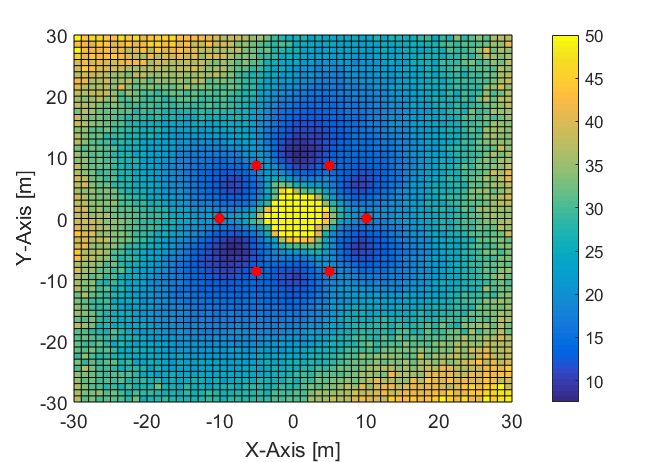
Figure 1: Matrix condition with BS 1 as reference.
Colours from yellow to blue: condition at the specific position. The red dots: base station positions..

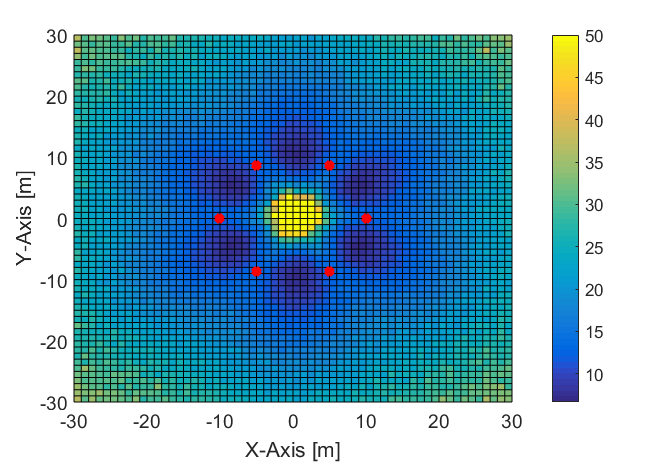
Figure 2: Matrix condition symmetric approach.
Colours from yellow to blue: condition at the specific position. The red dots: base station positions..

The position error of the previous method is subtracted from the new one at any position in the square area. Positive error differences indicate that the error with the second method is smaller. On the other hand, negative error difference shows that the error with the second approach is higher compared to the non-symmetrical solution. In the set-up presented, 56.11% have a positive error difference and 43.88% a negative one. Therefore, the second approach is 13% superior to the first one. In some test scenarios, where the geometrical constellation of the base stations is difficult for the lateration of the transponder position, the difference between the non-symmetrical and symmetrical approach increases by 30%. The first approach (non-symmetrical) always uses the same base station (base station one) from which the others are subtracted. If this transformation station is selected by the best condition of the coefficient matrix $||A||*||A^{-1}||$, the error difference between the new and previous approach is almost always a value between 50.44 % and 49.55 %. The increase in noise when selecting difficult geometrical constellations of the base stations leads to a higher difference between the symmetrical and non-symmetrical approach, with better results for the symmetrical approach. The condition of the coefficient matrix at different transponder positions can be seen in figure 1 and 2.

It can be observed that the coefficient matrix condition with the previous method, figure 1 is not symmetrical compared to the new approach figure 2. Base station selection with the best condition slightly changes the results but still underlies the symmetrical approach. The condition appears to be best in the area between the base stations. This is not always the case and depends on the base station constellation.

V Conclusion

’LPM’ is a nonlinear offset corrupted equation, whereby any transformation to a linear solution leads to a high noise impact on the outcome. We present a new numerically more stable direct solution, which is able to work with prefiltered data. In contrast to a non-filtered linear least square solution, this filtered direct solution is statically not correct, as not the data corrupted by Gaussian noise is used but the output of the filter. The results of this filtered direct solution are less influenced by the noise and therefore more suitable for use as starting values for the nonlinear solver. Furthermore, the symmetrical approach does not require a specific base station that is used for filtering, but instead all base stations play an equal part in finding a solution. The results of the new approach are at least 10 % better, compared to approaches whereby only the same base station is used. The best result for the first solution appears if the reference station that causes the best condition matrix is selected. In the new solution, there is no need to find the base station which causes the best matrix condition since every base station is used equally. Especially when the noise increases or the geometrical set-up is unfavourable, the results of the symmetrical approach are superior to its non-symmetrical counterpart.

References

- [1] J. S. Abel and J. W. Chaffee. Existence and uniqueness of gps solutions. IEEE Transactions on Aerospace and Electronic Systems, 27(6):952–956, Nov 1991.
- [2] S. Bancroft. An algebraic solution of the gps equations. IEEE Transactions on Aerospace and Electronic Systems, AES-21(1):56–59, Jan 1985.
- [3] J. Chaffee and J. Abel. On the exact solutions of pseudorange equations. IEEE Transactions on Aerospace and Electronic Systems, 30(4):1021–1030, Oct 1994.
- [4] R. Pfeil et al. Distributed fault detection for precise and robust local positioning. In In Proceedings of the 13th IAIN World Congress and Exhibition, 2009.
- [5] W. H. FOY. Position-location solutions by taylor-series estimation. IEEE Transactions on Aerospace and Electronic Systems, AES-12(2):187–194, March 1976.
- [6] R. Pfeil, S. Schuster, P. Scherz, A. Stelzer, and G. Stelzhammer. A robust position estimation algorithm for a local positioning measurement system. In Wireless Sensing, Local Positioning, and RFID, 2009. IMWS 2009. IEEE MTT-S International Microwave Workshop on, pages 1–4, Sept 2009.
- [7] K. Pourvoyeur, A. Stelzer, Alexander Fischer, and G. Gassenbauer. Adaptation of a 3-D local position measurement system for 1-D applications. In Radar Conference, 2005. EURAD 2005. European, pages 343–346, Oct 2005.
- [8] K. Pourvoyeur, A. Stelzer, T. Gahleitner, S. Schuster, and G. Gassenbauer. Effects of motion models and sensor data on the accuracy of the LPM positioning system. In Information Fusion, 2006 9th International Conference on, pages 1–7, July 2006.
- [9] K. Pourvoyeur, A. Stelzer, and G. Gassenbauer. Position estimation techniques for the local position measurement system LPM. In Microwave Conference, 2006. APMC 2006. Asia-Pacific, pages 1509–1514, Dec 2006.
- [10] A. Resch, R. Pfeil, M. Wegener, and A. Stelzer. Review of the LPM local positioning measurement system. In Localization and GNSS (ICL-GNSS), 2012 International Conference on, pages 1–5, June 2012.
- [11] J. Sidorenko, N. Scherer-Negenborn, M. Arens, and E. Michaelsen. Multilateration of the local position measurement. In 2016 International Conference on Indoor Positioning and Indoor Navigation (IPIN), pages 1–8, Oct 2016.
- [12] N. Sirola. Closed-form algorithms in mobile positioning: Myths and misconceptions. In 2010 7th Workshop on Positioning, Navigation and Communication, pages 38–44, March 2010.
- [13] A. Stelzer, K. Pourvoyeur, and A. Fischer. Concept and application of lpm - a novel 3-d local position measurement system. IEEE Transactions on Microwave Theory and Techniques, 52(12):2664–2669, Dec 2004.
- [14] Y. Zhou, C. L. Law, Y. L. Guan, and F. Chin. Indoor elliptical localization based on asynchronous uwb range measurement. IEEE Transactions on Instrumentation and Measurement, 60(1):248–257, Jan 2011.