Two-field cosmological models and the uniformization theorem

Abstract

We propose a class of two-field cosmological models derived from gravity coupled to non-linear sigma models whose target space is a non-compact and geometrically-finite hyperbolic surface, which provide a wide generalization of so-called $\alpha$-attractor models and can be studied using uniformization theory. We illustrate cosmological dynamics in such models for the case of the hyperbolic triply-punctured sphere.

1 Introduction

Inflation in the early universe can be described reasonably well by so-called cosmological $\alpha$-attractor models Escher ; Linde ; Linde3 , which provide a good fit to current observational results. The observational predictions of these models are to a large extent determined by the geometry of the scalar manifold rather than by the scalar potential.

The best studied $\alpha$-attractor models contain a single scalar field, being obtained by radial truncation of two-field models based on the hyperbolic disk Escher . The latter arise from cosmological solutions of 4-dimensional gravity coupled to a non-linear sigma model whose scalar manifold is the open unit disk endowed with its unique complete metric ${\mathcal{G}}$ of constant negative Gaussian curvature $K({\mathcal{G}})=-\frac{1}{3\alpha}$, where $\alpha$ is a positive parameter. As shown in Escher , the “universal” behavior of such models in the radial one-field truncation close to the conformal boundary of the disk is a consequence of the hyperbolic character of ${\mathcal{G}}$, when the scalar potential is “well-behaved” near the conformal boundary. It is thus natural to consider two-field $\alpha$-attractor models in which the hyperbolic disk is replaced by an arbitrary hyperbolic surface $\Sigma$ which is geometrically finite in the sense that its fundamental group is finitely-generated.

Definition 1

alpha A generalized two-field $\alpha$-attractor model is defined by a triplet $(\Sigma,{\mathcal{G}},V)$, where $(\Sigma,{\mathcal{G}})$ is a complete geometrically-finite hyperbolic surface and $V:\Sigma\rightarrow\mathbb{R}$ is a smooth potential function, while $K({\mathcal{G}})=-\frac{1}{3\alpha}$ with $\alpha>0$.

This class of models is very rich. Since in general $\Sigma$ has non-trivial topology, a complete understanding requires going beyond one field truncations. Instead, one can use the theoretical and numerical methods of PT1 ; Mul and certain other approximation techniques alpha .

2 Cosmological models with two real scalar fields minimally coupled to gravity

Let us recall the general description of cosmological models with two real scalar fields minimally coupled to gravity, allowing for scalar manifolds of non-trivial topology, in a global and coordinate-free description.

2.1 Einstein-Scalar theories with 2-dimensional scalar manifolds

Let $(\Sigma,{\mathcal{G}})$ be any oriented, connected, complete and possibly non-compact two-dimensional Riemannian manifold without boundary called the scalar manifold and $V\!:\!\Sigma\!\rightarrow\!\mathbb{R}$ be a smooth function called the scalar potential. We require completeness of the metric ${\mathcal{G}}$ in order to avoid problems with conservation of energy. For applications to cosmology, it is important to allow $(\Sigma,G)$ to be non-compact and of possibly infinite area.

Any triplet $(\Sigma,{\mathcal{G}},V)$ as above allows one to define an Einstein-Scalar theory on any four-dimensional oriented manifold $X$ which admits Lorentzian metrics. This theory includes 4-dimensional gravity (described by a Lorentzian metric $g$ defined on $X$) and a smooth map $\varphi:X\rightarrow\Sigma$ (which locally describes two real scalar fields), with action:

$$S[g,\varphi]=\int_{X}\mathcal{L}(g,\varphi)\mathrm{vol}_{g}~{}~{},$$ (1)

where $\mathrm{vol}_{g}$ is the volume form of $(X,g)$ and $\mathcal{L}(g,\varphi)$ is the Lagrange density:

$$\mathcal{L}(g,\varphi)=\frac{M^{2}}{2}\mathrm{R}(g)-\frac{1}{2}\mathrm{Tr}_{g}\varphi^{\ast}({\mathcal{G}})-V\circ\varphi~{}~{}.$$ (2)

Here $\mathrm{R}(g)$ is the scalar curvature of $g$ and $M$ is the reduced Planck mass. The quantity $\varphi^{\ast}({\mathcal{G}})$ is the pull-back through $\varphi$ of the metric ${\mathcal{G}}$, while $\mathrm{Tr}_{g}\varphi^{\ast}({\mathcal{G}})$ denotes the trace of the tensor field of type $(1,1)$ obtained by raising one of the indices of $\varphi^{\ast}({\mathcal{G}})$ using the metric $g$. The coordinate-free formulation (2) allows one to define such a theory globally for any topology of $\Sigma$ and $X$. The last two terms in the Lagrange density (2) describe the non-linear sigma model with source $(X,g)$, target space $(\Sigma,{\mathcal{G}})$ and scalar potential $V$.

2.2 Cosmological models defined by $(\Sigma,{\mathcal{G}},V)$

By definition, a cosmological model defined by $(\Sigma,{\mathcal{G}},V)$ is a solution of the equations of motion of the theory (1)-(2) when $(X,g)$ is a FLRW universe and $\varphi$ depends only on the cosmological time. We assume for simplicity that the spatial section is flat and simply connected. Hence the cosmological models of interest are defined by the following conditions:

1. $X$ is diffeomorphic with $\mathbb{R}^{4}$, with global coordinates $(t,x^{1},x^{2},x^{3})$.

2. The squared line element of $g$ has the form:

   $$\mathrm{d}s^{2}_{g}=-\mathrm{d}t^{2}+a(t)^{2}\sum_{i=1}^{3}{(\mathrm{d}x^{i})^{2}}~{}~{},~{}~{}\rm{with}~{}~{}a(t)>0~{}.$$

3. $\varphi$ depends only on $t$.

4. $(a(t),\varphi(t))$ are such that $(g,\varphi)$ is a solution of the equations of motion derived from (1).

With these assumptions, the cosmological equations of motion are:

$$\nabla_{t}\dot{\varphi}+3H\dot{\varphi}+(\mathrm{grad}_{{\mathcal{G}}}V)\circ\varphi=0~{},~{}~{}\frac{1}{3}\dot{H}+H^{2}-\frac{V\circ\varphi}{3M^{2}}=0~{},~{}~{}\dot{H}+\frac{\dot{\sigma}^{2}}{2M^{2}}=0~{},$$

where $\,\dot{~{}}\stackrel{{\scriptstyle{\rm def.}}}{{=}}\frac{\mathrm{d}}{\mathrm{d}t}~{},~{}\nabla_{t}\stackrel{{\scriptstyle{\rm def.}}}{{=}}\nabla_{\dot{\varphi}(t)}$ is the covariant derivative with respect to $\dot{\varphi}(t)$, $\sigma$ is the proper length parameter on the curve $\varphi(t)$, while $H\stackrel{{\scriptstyle{\rm def.}}}{{=}}\frac{\dot{a}}{a}$ denotes the Hubble parameter. The inflationary regions of a trajectory $\varphi(t)$ are defined as the time intervals for which the scale factor $a(t)$ is a convex and increasing function of $t$ ($\dot{a}>0,~{}\ddot{a}>0$) and are given by the condition:

$$H(t)<H_{c}(\varphi(t))~{},$$

where $H_{c}(p)\stackrel{{\scriptstyle{\rm def.}}}{{=}}\frac{1}{M}\sqrt{\frac{V(p)}{2}}$ is the critical Hubble parameter at a point $p\in\Sigma$. Approximations useful for studying such models are discussed in alpha .

2.3 Two-field generalized $\alpha$-attractor models

By definition, a hyperbolic surface is a connected, oriented, borderless and complete Riemannian two-manifold $(\Sigma,G)$ of constant Gaussian curvature equal to $-1$. A two-field generalized $\alpha$-attractor model is a two-field cosmological model defined by a triple $(\Sigma,{\mathcal{G}},V)$ as above, where ${\mathcal{G}}=3\alpha G$ with $\alpha$ a positive parameter and $(\Sigma,G)$ is a hyperbolic surface.

3 Uniformization of hyperbolic surfaces

An isometric model of the Poincaré disk is provided by the Poincaré half-plane, defined as the upper half-plane $\mathbb{H}\stackrel{{\scriptstyle{\rm def.}}}{{=}}\{\tau\in\mathbb{C}|~{}\mathrm{Im}\tau>0\}$ endowed with its unique complete hyperbolic metric $\mathrm{d}s_{\mathbb{H}}^{2}=\lambda^{2}_{\mathbb{H}}(\tau,\bar{\tau})\mathrm{d}\tau^{2}$, where $\lambda_{\mathbb{H}}(\tau,\bar{\tau})=\frac{1}{\mathrm{Im}\tau}$. The orientation-preserving isometries of $\mathbb{H}$ form the projective special linear group $\mathrm{PSL}(2,\mathbb{R})$. An element $A\in\mathrm{PSL}(2,\mathbb{R})$ is called elliptic if $|\mathrm{tr}(A)|<2$. By definition, a surface group is a discrete subgroup $\Gamma$ of $\mathrm{PSL}(2,\mathbb{R})$ which contains no elliptic elements. Our analysis of generalized $\alpha$-attractor models is based on the uniformization theorem unif :

Theorem 3.1

For any hyperbolic surface $(\Sigma,G)$ there is a surface group $\Gamma$ and a holomorphic covering map (uniformization map) $\pi_{\mathbb{H}}:\mathbb{H}\longrightarrow\Sigma$ defined on the Poincaré half-plane $\mathbb{H}$ such that $\Sigma$ is isometric to the quotient $\mathbb{H}/\Gamma$.

In this theorem, holomorphicity of $\pi_{\mathbb{H}}$ is understood with respect to the complex structure $J$ induced on $\Sigma$ by the conformal class of $G$.

3.1 Lifted trajectories and tilings

Consider the generalized $\alpha$-attractor model defined by a hyperbolic surface $(\Sigma,G)$ at a fixed positive value of the parameter $\alpha$. To study the cosmological trajectories $\varphi:\mathfrak{I}\longrightarrow\Sigma$ (where $\mathfrak{I}\subset\mathbb{R}$ is an interval), it is convenient to first study their lifts ${\widetilde{\varphi}}:\mathfrak{I}\longrightarrow\mathbb{H}$ to the hyperbolic plane and then project them back to $\Sigma$ as $\varphi=\pi_{\mathbb{H}}\circ{\widetilde{\varphi}}$. The projection from $\mathbb{H}$ to $\Sigma$ can be determined if we know the tiling of $\mathbb{H}$ determined by a fundamental polygon of $\Gamma$. There is no fully general stopping algorithm known for computing fundamental polygons of surface groups. However, a general algorithm polyg is known when $\Gamma$ is an arithmetic surface group such that $\mathbb{H}/\Gamma$ has finite hyperbolic area. The connection to uniformization theory shows that the study of generalized $\alpha$-attractor models requires sophisticated results from uniformization theory. When $\Sigma$ has finite hyperbolic area, this is closely connected to the theory of modular forms and hence to number theory.

3.2 The end and conformal compactifications

A non-compact hyperbolic surface $(\Sigma,G)$ has two natural compactifications, namely the end compactification ends of Freudenthal and Kerekjarto-Stoilow (which depends only on the topology of $\Sigma$) and the conformal compactification (which depends on the conformal class of the hyperbolic metric $G$). In the geometrically-finite case, these two compactifications can be described as follows:

• Since $\pi_{1}(\Sigma)$ is finitely-generated, $\Sigma$ is homeomorphic with $\widehat{\Sigma}\setminus\{p_{1},\ldots,p_{n}\}$, where $\widehat{\Sigma}$ is a closed oriented surface and $p_{1},\ldots,p_{n}$ are distinct points on $\widehat{\Sigma}$. The compact surface $\widehat{\Sigma}$ can be identified with the end compactification of $\Sigma$, while the points $p_{1},\ldots,p_{n}$ can be identified with the ends of $\Sigma$.

• As shown by Maskit, the conformal compactification $\bar{\Sigma}$ of $\Sigma$ (with respect to the complex structure $J$) can be identified with the topological closure of $\Sigma$ inside a closed Riemann surface which is obtained from $\Sigma$ by adding a finite number $n_{c}$ of points and a finite number $n_{f}$ of disks, where $n_{f}+n_{c}=n$. The topological boundary $\partial_{\infty}\Sigma=\bar{\Sigma}\setminus\Sigma$ consists of $n_{c}$ isolated points and $n_{f}$ disjoint simple closed curves and is called the conformal boundary of $\Sigma$. Contracting each of the $n_{f}$ curves to a point recovers the end compactification, the $n_{c}$ isolated points and the $n_{f}$ contraction points recovering the ends of $\Sigma$. Accordingly, the ends of $\Sigma$ divide into $n_{c}$ cusp ends (those corresponding to points in the conformal compactification) and $n_{f}$ flaring ends (those corresponding to simple closed curves in the conformal compactification).

On the neighborhoods of each end, the hyperbolic metric can be brought to one of four explicitly known forms (namely for the “cusp”, “funnel”, “horn” or “plane” end), thus providing the isometric classification of ends.

3.3 Well-behaved scalar potentials

Let $\widehat{\Sigma}$ be the end compactification of $\Sigma$. A scalar potential $V:\Sigma\rightarrow\mathbb{R}$ is called well-behaved at an end $p\in\widehat{\Sigma}\setminus\Sigma$ if there exists a smooth function ${\widehat{V}}_{p}:\Sigma\sqcup\{p\}\rightarrow\mathbb{R}$ such that $V={\widehat{V}}_{p}|_{\Sigma}$ . The potential $V$ is called globally well-behaved if it is well-behaved at each end of $\Sigma$, i.e. if there exists a globally-defined smooth function ${\widehat{V}}:\widehat{\Sigma}\rightarrow\mathbb{R}$ such that $V={\widehat{V}}|_{\Sigma}$.

3.4 Behavior near the ends

The cosmological equations of motion in semi-geodesic coordinates $(r,\theta)$ on an appropriate vicinity of an end $p\in\widehat{\Sigma}\setminus\Sigma$ reduce to alpha :

$$\ddot{r}-3\epsilon_{p}\alpha\left(\frac{C_{p}}{4\pi}\right)^{2}e^{2\epsilon_{p}r}\dot{\theta}^{2}+3H\dot{r}+\frac{1}{3\alpha}\partial_{r}V=0~{}~{},$$

$$\ddot{\theta}+2\epsilon_{p}\dot{r}\dot{\theta}+3H\dot{\theta}+\frac{1}{3\alpha}\left(\frac{4\pi}{C_{p}}\right)^{2}e^{-2\epsilon_{p}r}\partial_{\theta}V=0~{}~{},$$

where $C_{p}$ and $\epsilon_{p}$ are known constants depending on the type of end. Since $\theta$ is periodic, a generic trajectory will spiral around the ends for any well-behaved scalar potential. Using an argument similar to that of Linde3 , we showed in alpha that generalized $\alpha$-attractor models have the same kind of ”universal” behavior as the disk models of Escher in the naive one field truncation near each end obtained by fixing $\theta$. The cosmological behavior away from the ends is much more subtle than that of ordinary $\alpha$-attractors; some of its qualitative features were discussed in alpha . Various examples are discussed in elem ; modular .

4 Examples of trajectories for the hyperbolic triply punctured sphere

Consider those generalized $\alpha$-attractor models for which the scalar manifold $\Sigma$ is the triply-punctured Riemann sphere (a.k.a. the modular curve) $Y(2)\stackrel{{\scriptstyle{\rm def.}}}{{=}}\mathbb{C}\mathbb{P}^{1}\setminus\{p_{1},p_{2},p_{3}\}$. This is diffeomorphic with the doubly-punctured complex plane endowed with its complete hyperbolic metric $\mathrm{d}s^{2}=\rho(\zeta,\bar{\zeta})^{2}\mathrm{d}\zeta^{2}$, where:

$$\rho(\zeta,{\bar{\zeta}})=\frac{\pi}{8|\zeta(1-\zeta)|}\,\frac{1}{\mathrm{Re}[\mathcal{K}(\zeta)\mathcal{K}(1-\bar{\zeta})]}~{}~{},~{}~{}\mathcal{K}(\zeta)=\int_{0}^{1}\frac{\mathrm{d}t}{\sqrt{(1-t^{2})(1-\zeta t^{2})}}~{}.$$

Each of the three punctures $p_{i}$ corresponds to a cusp end, so the end compactification is ${\widehat{\Sigma}}=\mathbb{C}\mathbb{P}^{1}\simeq\mathrm{S}^{2}$. The surface $Y(2)$ is uniformized by the principal congruence subgroup of level $2$, $\Gamma(2)\!=\!\Big{\{}A\!=\!\left[\begin{array}[]{cc}a&b\\ c&d\end{array}\right]\in\mathrm{PSL}(2,\mathbb{Z})~{}|~{}a,d=\mathrm{odd}\,,~{}b,c=\mathrm{even}\Big{\}}\,$, with uniformization map given by the elliptic modular lambda function $\pi_{\mathbb{H}}(\tau)\!\equiv\!\lambda(\tau)\!=\!\frac{\wp_{\tau}(\frac{1+\tau}{2})-\wp_{\tau}(\frac{\tau}{2})}{\wp_{\tau}(\frac{1}{2})-\wp_{\tau}(\frac{\tau}{2})}~{},$ where $\wp$ is the Weierstrass elliptic function of modulus $\tau$. A fundamental polygon for the action of $\Gamma(2)$ on $\mathbb{H}$ is given by the hyperbolic quadrilateral $\mathfrak{D}_{\mathbb{H}}=\{\tau\in\mathbb{H}|-1<\mathrm{Re}\tau<0,|\tau+\frac{1}{2}|>\frac{1}{2}\}\cup\{\tau\in\mathbb{H}|0\leq\mathrm{Re}\tau<1,|\tau-\frac{1}{2}|>\frac{1}{2}\}$.

Consider the following two globally well-behaved scalar potentials:

$${\widehat{V}}_{0}(\psi,\theta) \stackrel{{\scriptstyle{\rm def.}}}{{=}} M_{0}(1+\sin\psi\cos\theta)~{}~{},$$

$${\widehat{V}}_{+}(\psi) \stackrel{{\scriptstyle{\rm def.}}}{{=}} M_{0}\cos^{2}\frac{\psi}{2}~{}~{},$$

where $M_{0}\stackrel{{\scriptstyle{\rm def.}}}{{=}}M\sqrt{2/3}$ and $\psi,\theta$ are spherical coordinates on the end compactification $\widehat{\Sigma}=\mathrm{S}^{2}$. Fixing $\alpha=\frac{1}{3}$ and choosing the initial conditions $\tau_{0}$ and ${\widetilde{v}}_{0}\stackrel{{\scriptstyle{\rm def.}}}{{=}}\dot{\widetilde{\varphi}}(t_{0})$ given in Table 4, we compute modular the lifted trajectories on the Poincaré half-plane with coordinate $\tau=x+\mathbf{i}y$ and then project them to $Y(2)$ (see Figs. 1 and 2). The potentials ${\widehat{V}}_{0}$ and respectively ${\widehat{V}}_{+}$ correspond to ${\widetilde{V}}_{0}$ and ${\widetilde{V}}_{+}$ on $\mathbb{H}$ and to $V_{0}$ and $V_{+}$ on $Y(2)$.

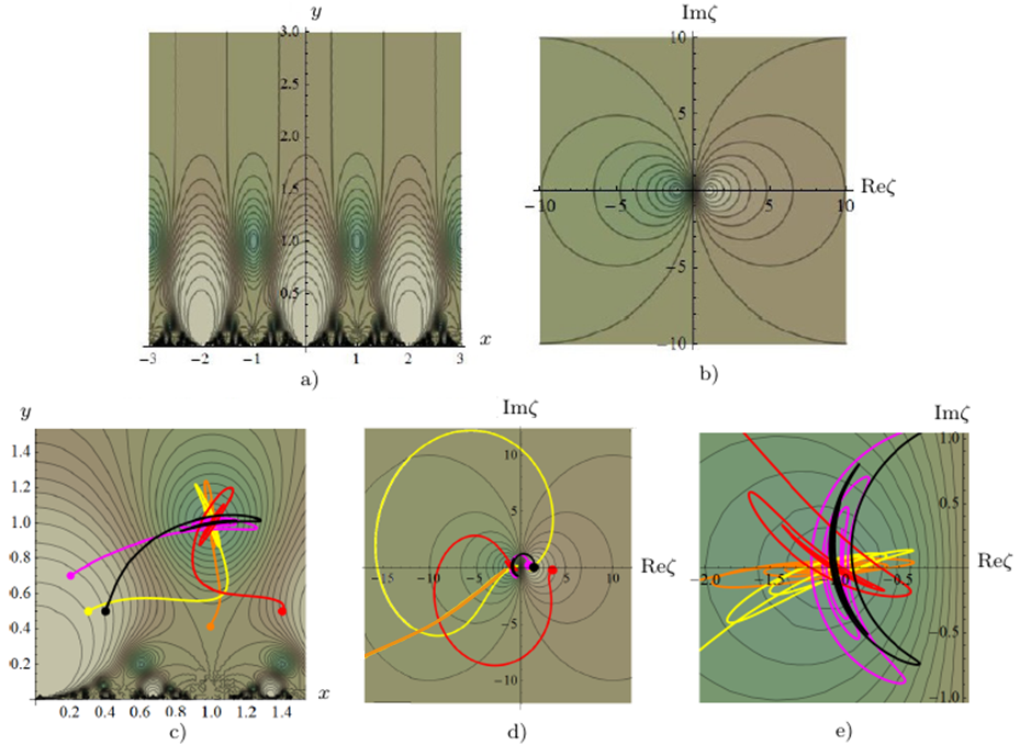
Figure 1: a) Level plot of the lifted potential ${\widetilde{V}}_{0}$ on $\mathbb{H}$. b) Level plot of $V_{0}$ on $Y(2)$. c) Lifted trajectories on $\mathbb{H}$, with initial conditions given in Table 1. d) Projected trajectories on $Y(2)$, where the orange trajectory is too long to fit into the plot at the scale shown. e) Detail of the spiral ends of the trajectories on $Y(2)$. The beginning points of the trajectories are indicated by fat dots. In all figures, dark green indicates minima of the potential while light brown indicates maxima.

For the potential ${\widetilde{V}}_{0}$, we find that the red, magenta, yellow and orange trajectories start in inflationary regime (see Fig. 3), but computations show they have small number of e-folds (less than 5); on the other hand, the black trajectory is not inflationary. For potential ${\widetilde{V}}_{+}$, we find that the red, yellow and orange trajectories (see Fig. 4) start in inflationary regime, while the magenta and black trajectories are not inflationary. The orange trajectory has 50 e-folds and using very small variations of its initial conditions given in Table 1 we can easily find other trajectories with 50-60 e-folds; this shows that generalized $\alpha$ attractors with $\Sigma=Y(2)$ can produce phenomenologically realistic predictions. The number of e-folds is given by $N=\int_{0}^{t_{I}}H(t)\mathrm{d}t$, where $t_{I}$ is the inflationary period (the duration of the first inflationary regime).

Table 1: Initial conditions on the Poincaré half-plane.

trajectory	$\tau_{0}$	${\widetilde{v}}_{0}$
black	$0.4+0.5\mathbf{i}$	$0.3+\mathbf{i}$
red	$1.4+0.5\mathbf{i}$	$0.1+0.2\mathbf{i}$
magenta	$0.2+0.7\mathbf{i}$	$0.7+0.5\mathbf{i}$
yellow	$0.3+0.5\mathbf{i}$	$0$
orange	$0.99+0.415\mathbf{i}$	$0$

Figure 2: a) Level plots of the lifted potential ${\widetilde{V}}_{+}$ on $\mathbb{H}$ and the lifted trajectories with initial conditions given in Table 1. b) Level plots of $V_{+}$ on $Y(2)$ and the corresponding projected trajectories. c) The full orange trajectory projected on $Y(2)$.

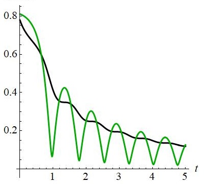
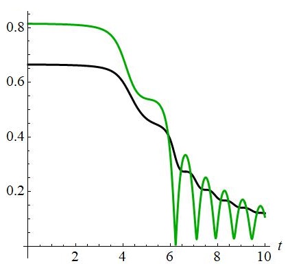
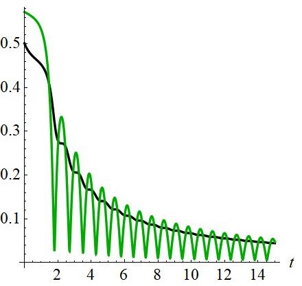
Figure 3: Plot of $H(t)/\sqrt{M_{0}}$ (black) and $H_{c}(t)/\sqrt{M_{0}}$ (green) for the red, magenta, yellow and orange trajectories for the potential ${\widetilde{V}}_{0}$.

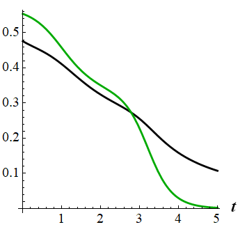
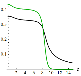
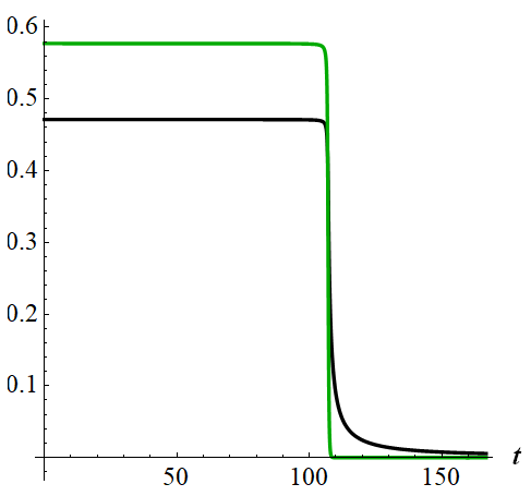
Figure 4: Plot of $H(t)/\sqrt{M_{0}}$ (black) and $H_{c}(t)/\sqrt{M_{0}}$ (green) for the red, yellow and orange trajectories in the potential ${\widetilde{V}}_{+}$. The red and yellow trajectorie have small number of e-folds (less than 2), but the orange trajectory has 50 e-folds.

5 Conclusions

We proposed alpha ; modular ; elem a wide generalization of two-field $\alpha$-attractor models obtained by promoting the scalar manifold from the Poincaré disk to an arbitrary geometrically finite non-compact hyperbolic surface and a procedure for studying such models through uniformization techniques. Our models are parameterized by a constant $\alpha>0$, by the choice of a surface group $\Gamma$ and of a smooth scalar potential $V$. They have the same universal behavior as ordinary $\alpha$-attractors in the naive one-field truncation near each end, provided that the scalar potential is well-behaved near that end.

- (1) E. M. Babalic, C. I. Lazaroiu, Generalized -attractors from the hyperbolic triply-punctured sphere, arXiv:1703.01650 [hep-th].
- (2) E. M. Babalic, C. I. Lazaroiu, Generalized -attractor models from elementary hyperbolic surfaces, arXiv:1703.01650 [hep-th].
- (3) C. I. Lazaroiu, C. S. Shahbazi, Generalized -attractor models from geometrically finite hyperbolic surfaces, arXiv:1702.06484 [hep-th].
- (4) M. Dias, J. Frazer, D. J. Mulryne, D. Seery, JCAP 12 (2016) 033.
- (5) R. Kallosh, A. Linde, Comptes Rendus Physique 16 (2015) 914.
- (6) R. Kallosh, A. Linde, D. Roest, JHEP 11 (2013) 098.
- (7) M. Galante, R. Kallosh, A. Linde, D. Roest, Phys. Rev. Lett. 114 (2015) 141302.
- (8) C. M. Peterson, M. Tegmark, Phys. Rev. D 83 (2011) 023522.
- (9) I. Richards, Transactions of the AMS 106 (1963) 2, 259–269.
- (10) J. Voight, J. Théorie Nombres Bordeaux 21 (2009) 2, 467–489.
- (11) H. P. de Saint-Gervais, Uniformization of Riemann Surfaces: revisiting a hundred-year-old theorem, EMS, 2016.