Planning with Pixels in (Almost) Real Time

Abstract

Recently, width-based planning methods have been shown to yield state-of-the-art results in the Atari 2600 video games. For this, the states were associated with the (RAM) memory states of the simulator. In this work, we consider the same planning problem but using the screen instead. By using the same visual inputs, the planning results can be compared with those of humans and learning methods. We show that the planning approach, out of the box and without training, results in scores that compare well with those obtained by humans and learning methods, and moreover, by developing an episodic, rollout version of the IW($k$) algorithm, we show that such scores can be obtained in almost real time.

Introduction

The Atari 2600 video games supported in the ALE environment (?) provide a challenging set of benchmarks for reinforcement learning (RL) and planning algorithms. The breakthrough results achieved by the deep reinforcement algorithm DQN (?) made it to the popular press, and were followed by similar results obtained using more standard (shallow) RL methods operating on suitably defined screen features (?).

The learning and planning settings for ALE deal with the same games but compute different forms of control. Learning is done off-line and results in close-loop controllers that require no lookahead. Planning, on the other hand, is done on-line: an action is selected by looking ahead in the future, the action is applied, and the process iterates until the game terminates or a maximum number of frames is reached. The learning approach is slow but the selection of actions, once the controller has been learned, is very fast. The planning approach, on the other hand works right out of the box without training but results in a selection of actions that is slower. Another difference is that the planning approaches (?; ?), unlike the reported RL approaches, plan with the (RAM) memory states of the Atari emulator using information that is not available to humans.

In this work, we address some of the limitations of current planning approaches to the Atari games, so that the resulting scores can be compared with those achieved by humans and learning methods. For this, planning is performed using the visible information from the screen. The “screen states” are associated with the values of a set of boolean pixel features called B-PROST (?), defined and motivated by the neural net architecture underlying the successful DQN algorithm. The number of feature bits in B-PROST is more than 20,000,000, and the number of possible screen states is exponential in this number. Yet, while the complexity of planning algorithms like breadth-first search grows with the number of reachable states, the complexity of algorithms such as IW(1) (?) is linear in the number of features.

We show that the IW(1) planning algorithm using the B-PROST pixel features turns out to achieve scores that compare well with those reported for humans and learning algorithms. Our main focus, however, will be on achieving such scores by planning over very short time windows, approaching real-time play. For this, we formulate an episodic, rollout version of IW($k$) and show that it has a much better anytime behavior than IW($k$). Rollout IW($k$) is not a systematic tree-search algorithm like IW($k$), but a sequence of rollouts or episodes reminiscent of (open loop) Monte Carlo algorithms, all starting in the same node, each one given by a sequence of actions. The sequence of rollouts is designed to emulate IW($k$) in polynomial time. More precisely, if a goal has width $k$ (?), Rollout IW($k$) will reach the goal in a polynomial number of rollouts.

The empirical results show that Rollout IW(1) achieves scores comparable to those of humans and RL algorithms almost in real-time: decisions are made in 0.5 seconds using a frameskip of 15 that would require decisions made in 0.25 seconds for real-time play. The results involve other simple extensions of IW(1) that are also discussed.

The paper is organized as follows. We review ALE, IW planning, and the B-PROST visual feature set, and then consider Rollout IW, extensions, and the experimental results.

Planning and Model

ALE supports a planning and a learning setting. In the planning setting, the agent performs a lookahead using the simulator, selects and applies an action, and the process iterates until the game terminates or a given number of frames is reached. Often a frameskip of $N$ is used, meaning that decisions are made every $N$ frames with the last decision repeated over the following $N\!-\!1$ frames.

The simulator returns reward (score) information and the goal is to maximize overall reward. When planning with memory states, the only planning setting originally supported in ALE, the agent has access to the system (RAM) state. The lookahead from a state $s_{0}$ is aimed at finding a sequence of actions and states $s_{0},a_{0},s_{1},a_{1},\ldots,a_{n-1},s_{n}$ with high reward. The state at step $i$ is $s_{i+1}=f(a_{i},s_{i})$ and the reward at step $i+1$ is $r_{i+1}=r(s_{i-1},a_{i},s_{i})$, where $f$ is the deterministic state transition function, and $r$ is the deterministic reward function, both a priori unknown. The reward $r_{i+1}$ is observable and the system states $s_{i+1}$ are observable in the memory setting. The score obtained along an action sequence is the sum of the observed rewards, and the discounted score refers to the discounted sum of rewards with a discount factor slightly less than 1 that favors rewards that are closer in time. Different planning algorithms manage to explore the value of different action sequences, and the action selected is the one that starts the sequence with highest score. The screen setting is similar except that the RAM states are not observable. Instead, the screen of the game is observable but is less informed than the RAM memory because the former is determined by the latter and there may be different states associated with the same screen. The planning task, however, is similar: to find an action sequence that results in a high score.

Planning with IW

IW(1) is a simple “classical” planning algorithm defined over states that determine the value of a given set of boolean features or atoms $F$ (?). Starting with a given initial state $s_{0}$, IW(1) is a standard breadth-first search from $s_{0}$ with one change: if upon generation of a state $s$, there is no feature $f_{i}$ in $F$ such that $f_{i}$ is true in $s$ and false in all the states generated before $s$, the state $s$ is pruned. In other words, the only states that are not pruned are those that make some feature in $F$ true for the first time. Such states are said to have novelty $1$. The number of states expanded in the IW(1) search is thus linear in the size of the feature set and not in the number of states as in standard breadth-first search. The algorithm IW($k$) is the algorithm IW(1) but applied to the larger feature set $F^{k}$ made up of the conjunctions of $k$ features from $F$.

In classical planning, the set $F$ of features commonly used is the set of atoms for the task. Basic properties of IW($k$) are that many planning benchmark domains have a bounded and small width $w$ no greater than 2 when goals are single atoms, and that such instances are solved optimally (shortest plans) by running IW($w$) in low polynomial time in the number of atoms. For example, the goal $on(x,y)$ for any two blocks $x$ and $y$ in Blocksworld can be shown to have width no greater than $2$, no matter the number of blocks or initial configuration. This means that IW(2) finds an optimal (shortest) plan to achieve $on(x,y)$ in polynomial time in the number of atoms and blocks even though the state space for the problem is exponential in both. The same is true for most classical planning benchmarks. The majority of the benchmarks, however, do not feature a single atomic goal but a conjunction of them, and a number of extensions of IW($k$) have been developed aimed at problems with conjunctive goals, some of which represent the current state of the art in classical planning (?; ?). Since these algorithms can work with simulators, variations of IW($k$) have been used in other settings such as the general-video game competition (?), and task and motion planning problems in robotics (?).

Planning with Memory States

Among the original planning baselines, random playing and breadth-first search achieve very low scores, and only UCT (?) does well. IW(1) was shown to improve the performance of UCT using the 128 bytes of memory as features (?). The alternative representation where the boolean features are associated with each one of the 1024 bits in memory makes IW(1) runs faster but with poorer results. The IW algorithms are purely exploratory and do not take rewards into account for focusing the search. In order to improve the scores achieved by IW(1), two variants were proposed, 2BFS, a best-first search algorithm (?), and prioritized IW(1) (?), that managed to improve the scores substantially. From a theoretical point of view, however, unlike IW($k$), neither 2BFS nor prioritized IW(1) run in polynomial time in the number of features.

Planning with Pixels

The sensory input in ALE is given by images defined by a pixel array 160 wide and 210 high, with pixels that may have up to 128 colors. In principle, we can use the resulting set of $160\times 210\times 128$ booleans as the set of features in IW, yet the performance of IW, like the performance of learning algorithms, is sensible to the choice of features. Features that capture meaningful structure normally yield better results than raw features that do not. For this reason, screen pixels are mapped into the set of visual features B-PROST defined by ? for ALE, which are motivated by the design choices in the DQN architecture.

The Atari screen is split into $16\times 14$ disjoint tiles, each comprised of $10\times 15$ pixel patch. For each tile $(i,j$) and color $c$, there is a basic feature $f_{i,j,c}$ which is 1 (true) iff the image contains a pixel of color $c$ in the tile $(i,j)$. The number of basic features is $\text{28,672}=16\times 14\times 128$.

The basic pairwise relative offsets in space features (B-PROS) track relative distances among pairs of basic features. A B-PROS feature $f_{i,j,c,c^{\prime}}$ is 1 iff there is a pixel of color $c$ in tile $t$ and a pixel of color $c^{\prime}$ in tile $t^{\prime}$ such that the horizontal and vertical offsets of $t^{\prime}$ in relation to $t$ are $i$ and $j$, for $-13\leq i\leq 13$ and $-15\leq j\leq 15$. The number of non-redundant B-PROS features is $\text{6,856,768}=(\text{28,672}+((31\times 27\times 128^{2}-128)/2+128))$.

Finally, the basic pairwise relative offsets in time features (B-PROT) represent pairwise relative offsets between basic features obtained from the screen at two different time points: the current and previous decision times (recall that decisions are made at intervals given by the frameskip parameter). More specifically, the B-PROT feature $f^{\prime}_{i,j,c,c^{\prime}}$ is 1 iff there is a pixel of color $c$ in tile $t$ at the previous decision point and a pixel of color $c^{\prime}$ in tile $t^{\prime}$ at the current decision point such that the offsets of $t^{\prime}$ in relation to $t$ are $i$ and $j$. B-PROT features are non-Markovian, and hence the “screen state” contains information about the previous screen too. The number of B-PROT features is $\text{13,713,408}=31\times 27\times 128^{2}$, which is twice the number of B-PROS features as there are no redundant pairs.

The B-PROST feature set contains the Basic, B-PROS, and B-PROT sets for a total of 20,598,848 features. ? go on to introduce additional features aimed at grouping pixels into object-like blobs. While in our results we compare with their RL algorithm working on their full set of Blob-PROST features, we stick to the simpler B-PROST set. An analysis of the impact of different visual features on the performance of the planning algorithms would be interesting but is beyond the scope of this work.

Two final comments about the use of the visual features. Following ? and previous work, background pixels are removed from the screen, a transformation that is like removing “static” atoms from a planning problem. A background pixel is one that preserves its color in all reachable screens and it is “removed” by “painting” it with a common “background” color. This reduces the number of active features (features with value $1$). Background pixels are identified dynamically as the game evolves. A first set of background pixels is identified by performing 100 random actions. Then, every time a screen is scanned for computing the features of a state, the background status of each pixel is updated by comparing the pixel value with a stored value.

The “states” in IW(1) and the variants introduced below refer to the state of the B-PROST features. There are potentially $128^{160\times 210}$ different screen configurations but IW(1) is guaranteed to expand 20,598,848 states at most, but usually much fewer as the features are sparse and most combinations of them never become true.

IW Rollouts

While IW(1) is a low polynomial time algorithm whose effectiveness has been shown in classical planning and games, its suitability for real-time game playing, where actions have to be taken in a few hundred milliseconds, is limited by the underlying breadth-first search. IW(1) can search much deeper than breadth-first search over a limited time window, but if the window is small, nodes that are beyond a certain depth will not be explored either. Since a main goal of this work is to play the Atari 2600 games in real time, we introduce an alternative to IW(1), called Rollout IW(1), that does not have this limitation and has a much better anytime behavior. In addition, Rollout IW(1) asks less from the simulator: while tree search algorithms like IW(1) need the facility of expanding nodes, i.e., of applying all actions to a node, the rollouts in Rollout IW(1) apply just one action per node. We will prove that Rollout IW(1) terminates in polynomial time, reaching every width 1 goal optimally (length-wise) like IW(1). While the description and the results below are for Rollout IW($k$) with $k=1$, the generalization to higher values of $k$ is direct: for this, the set of boolean features $F$ is replaced by the larger set $F^{k}$ of features comprised of the conjunctions of $k$ features from $F$.

Given a root node defined by an initial state, a sequence of rollouts starting at the root node determines a tree. A rollout is an action sequence, and a node in the tree stands for the set of state-action trajectories generated by the rollouts that share a common prefix and end with the same state, which is the state associated with the node. The edges of the tree are the actions. For the sequence of rollouts to replace the breadth-first construction of the tree, Rollout IW(1) considers “extended features” ${(f,d)}$ where $f$ is a feature in $F$ and $d$ is an integer in $0\leq d\leq|F|$. A trajectory $\tau$ ending in a state $s$ makes the extended feature (e-feature) ${(f,d)}$ true iff $s$ makes $f$ true, and the length of the path as measured by the number of actions in $\tau$ is $d$. In addition, the min $d$ value over all the e-features ${(f,d)}$ reached is stored as $d[f]$ for each feature $f\in F$. This value is initially $0$ for features $f$ true in the root state and $\infty$ otherwise.

Generate-Lookahead-Tree:

begin

       $d:=\text{make-empty-table}()$

       $r:=\text{make-root-node}()$

       while $r$ isn’t solved and still within budget do

             $\text{Rollout}(r,d)$

      

$\text{Rollout}(n,d)$:

begin

       $\text{Fill-Node}(n)$

       while $n$ isn’t solved do

             if $n$ isn’t expanded then  $\text{Expand}(n)$

             $n:=\text{Pick random unsolved child of $n$}$

             $\text{Fill-Node}(n)$

            if $n$ is terminal then

                   $n.visited:=\textbf{true}$

                   $\text{Solve-and-Propagate-Label}(n)$

                   break

             else

                   $f:=\text{Get-Novel-Feature}(n,d)$

                   if $n.depth<d[f]$ then

                         /* case 1 */

                         $n.visited:=true$

                         $\text{Update-Feature-Table}(d,n)$

                   else if $\neg n.visited\,\land\,n.depth\geq d[f]$ then

                         /* case 2 */

                         $n.visited:=true$

                         $\text{Solve-and-Propagate-Label}(n)$

                         break

                   else if $n.visited\,\land\,d[f]<n.depth$ then

                         /* case 3 */

                         $\text{Solve-and-Propagate-Label}(n)$

                         break

                   else

                         /* case 4: continue extending rollout */

                        

                  

            

      

Algorithm 1 Pseudo-code of Rollout IW(1).

Nodes in the tree can be labeled as SOLVED. Initially, the tree contains the root node only and the algorithm terminates when this node is SOLVED or the time budget for selecting an action is over. In order to define the Rollout IW(1) algorithm fully (pseudo-code shown in Figure 1), four aspects must be made precise: A) how actions are selected in rollouts, B) how rollouts are terminated, C) how nodes are labeled SOLVED, and D) how labels propagate up in the tree.

Rollouts start in the root node, and recursively extend a path prefix $\tau^{\prime}$ with an action $a$ and a node $n$ representing a state $s$. The resulting path $\tau={\langle\tau^{\prime},a,n\rangle}$ may already be in the tree or not: if it is in the tree, the only condition in the choice of the action $a$ is that node $n$ is not labeled SOLVED. A rollout can select any action in a node as long as it does not lead to a SOLVED node. Four cases are distinguished after extending a rollout with a new action. In two of these cases the rollout is terminated, the tip nodes are labeled SOLVED, and the label is propagated up the tree. In the other two cases, the rollout is extended with a new action and the process iterates. If $\tau={\langle\tau^{\prime},a,n\rangle}$ is the tree branch that results from extending a rollout with an action $a$, the four cases are:

1. Case 1: if node $n$ is new in the tree and makes some e-feature $(f,d)$ true with $d<d[f]$, continue rollout.

2. Case 2: if node $n$ is new in the tree but $d\geq d[f]$ for each e-feature $(d,f)$ true in $n$, terminate rollout.

3. Case 3: if node $n$ is already in the tree but for no e-feature $(f,d)$ true in $n$, $d=d[f]$, terminate rollout.

4. Case 4: if node $n$ is already in the tree and makes some e-feature $(f,d)$ true with $d=d[f]$, continue rollout,

Cases 1 and 2 involve a new branch in the tree, leading to a new node. The rollout terminates in the node, if the node does not bring a “new” extended feature, which is a pair $(f,d)$ that improves the distance to $f$, i.e., with $d<d[f]$. Cases 3 and 4 are different. Since Rollout IW(1) is based on rollouts and not on tree search like IW(1), it means that it has to search multiple times beneath a node $n$ in order to explore each of its children. In such cases, $n$ is not a new node in the tree but an existing node. The search beneath such nodes is terminated when for all e-features $(f,d)$ true in $n$, the distance $d$ to $f$ can be shown not to be the shortest given the search so far.

In Case 1, the table $d$ that tracks the shortest distances to features $f$ is updated by setting $d[f]$ to the minimum between $d[f]$ and the depth of $n$, for each feature $f$ true in $n$. In Cases 2 and 3, the last node $n$ of the rollout is labeled as SOLVED and the label is propagated up the tree. Nodes in the tree become SOLVED when all of their children have been generated and all of them have been labeled as SOLVED.

In the code shown in Figure 1, the procedure Get-Novel-Feature() returns any feature $f$ for a pair $(f,d)$ true in $n$ with $d<d[f]$, if one exists, else any feature $f$ with $d=d[f]$ if one exists, and any feature otherwise. The Fill-Node() procedure fills up the data structure and calls the simulator except when the state is cached (see below). A basic property of the sequence of rollouts is:

Theorem 1.

Each rollout improves the distance $d$ to some feature $f$, i.e. it reaches an e-feature $(f,d)$ with $d<d[f]$, or labels the child of a node in the tree as SOLVED.

The length of rollouts is bounded by $|F|$ as for every non-tip node, $d\leq d[f]$ must be true for some feature $f$, yet $d$ grows monotonically along the rollout while $d[f]$ doesn’t grow. Similarly, the number of nodes in the tree is always bounded by the total number $|F|^{2}$ of e-features $(f,d)$, as each new node must improve $d[f]$ for some feature $f$. Theorem 1 implies then that:

Theorem 2.

Rollout IW(1) terminates (root node SOLVED) in a number of rollouts bounded by $|F|^{2}\times b$ where $b$ is the branching factor (maximum number of actions that can be applied at a give node).

Since IW(1) can generate up to $|F|\times b$ nodes, Rollout IW(1) involves an overhead. Rollout IW(1) does not compete with plain IW(1) when both are run to completion but it is an appealing alternative over short time windows.

In order to characterize the states that are reached by Rollout IW(1) from a given state $s_{0}$, we appeal to the notion of width from (?): a goal $G$ defined from the features in $F$ has width 1 iff there is a trajectory $s_{0},a_{0},\ldots,a_{n-1},s_{n}$ where $G$ is true in $s_{n}$, $n>0$, such that for each state $s_{i}$ in the trajectory: 1) the prefix $s_{0},a_{0},\ldots,s_{i}$ is optimal for some feature $f_{i}$ (no other trajectory reaches $f_{i}$ with less number of actions), 2) any optimal trajectory to $f_{i}$ can be extended into an optimal trajectory for $f_{i+1}$, and 3) the optimal plans for $f_{n}$ are optimal for $G$. IW(1) is guaranteed to reach all width 1 goals no matter how the children nodes are ordered in the underlying breadth-first search. The same is true for Rollout IW(1):

Theorem 3.

Rollout IW(1) is guaranteed to reach every width 1 goal in time that is polynomial in the number of features.

The practical value of Rollout IW(1), however, is its anytime behavior that follows from replacing the breadth-first search in plain IW(1) by depth-progressing rollouts. As mentioned above, all definitions and properties carry easily to Rollout IW($k$) for $k>1$.

Extensions and Variations

Before testing IW(1) and its rollout version, we consider one optimization and two variations.

Partial Caching

On-line planning schemes for the Atari games have appealed to different ways of using previous lookahead results in the current lookahead (?). Indeed, once an action has been selected and applied, the subtree rooted at the selected child contains information that can be used “for free” in the new lookahead. In the IW(1) planning scheme of ? (?), that operates over the RAM states, if the lookahead tree in a given situation involves the trajectory $s_{0},a_{0},s_{1},a_{1},\ldots,s_{n}$ and the action $a_{0}$ is selected and applied, the sub-branch $s_{1},a_{1},\ldots,s_{n}$ is used for both avoiding simulator calls (it can be predicted that the action sequence $a_{1},\ldots,a_{i-1}$ will lead to the state $s_{i}$), and for adding extra states to the search (states along such cached branches are not pruned and are not used for updating the novelty table). In the screen setting, we do the same but replace the RAM states with screen states. There is however an important change: if $s_{1},a_{1},\ldots,s_{n}$ is a cached path made of screen states rather than memory states, then predicting the next screen state $s_{i+1}$ after an action $a_{n}$ when the path $s_{1},a_{1},\ldots,s_{n},a_{n},s_{n+1}$ is not cached may involve up to $n$ simulator calls because the screen state $s_{n+1}$ can only be obtained by using the simulator from the root state. In order to avoid these repeated calls we assume an “intelligent” simulator that caches such states within the same lookahead tree, while keeping them hidden from the planning agent.

Penalties and Risk Aversion

In the ALE setting, the planning agent observes when he dies, and there are games, such as Breakout, on which the loss of a life does not generate a negative reward (penalty). In other games, positive and negative rewards are not calibrated. For example, in Space Invaders, losing a life results in a reward of -1 while shooting an “alien” results in a reward of 5 or higher. This results in situations where the lookahead does not find sufficiently high rewards, or the planning agent may select actions leading to an early and unnecessary death. To avoid this, negative rewards are multiplied by a large constant $\alpha=\text{50,000}$ and a high negative reward of $-10\alpha$ is used for deaths. Since this form of “reward shaping” appears to be fair for comparing with humans but less so for comparing with learners, we report results with and without this “risk averse” transformation.

From Subgoaling to Subscoring

The IW($k$) algorithm is effective for achieving atomic goals in classical planning but not for achieving sets $G$ of atomic goals (?). A variation of IW($k$), that we call $\textrm{IW}_{G}(k)$, provides a simple mechanism for doing that, and will serve as the basis for making a score-sensitive IW algorithm that is also polynomial. In the implementation of IW(1), a state $s$ has novelty 1 iff there is a true feature $f$ in $s$ that is not marked as “reached” in a novelty table that tracks the features that have been reached so far. $\textrm{IW}_{G}(1)$ is like IW(1) but with one change: there are $|G|$ novelty tables, with the $k$-th table tracking the features that have been reached by the states that make exactly $k$ goals true (?). A state $s$ has novelty 1 in $\textrm{IW}_{G}(1)$ iff there is a true feature $f$ in $s$ that is not marked as “reached” in the $k$-th novelty table where $k=\#g(s)$ is the number of goals that are true in $s$. Like IW(1), $\textrm{IW}_{G}(1)$ is a breadth-first search but while IW(1) expands up to $|F|$ nodes, $\textrm{IW}_{G}(1)$ can expand up to $|F|\times|G|$ nodes.

IW(1) with subscoring, denoted as $\textrm{IW}_{S}$(1) is similar to IW(1) with subgoaling, namely $\textrm{IW}_{G}$(1), but with the goal counter $\#g(s)$ replaced by the integer-valued $logscore(s)$ whose value approximates the logarithm base 2 of the score (reward) accrued on the unique path leading to state $s$. A state has novelty 1 in $\textrm{IW}_{S}$(1) iff there is a feature $f$ true in $s$ that is not marked as reached in the $k$-th table for $k=\text{logscore}(s)$.

The scoring function is as follows. If the reward $r(s)$ of the path leading to $s$ is non-positive, $\text{logscore}(s)=0$. Else, if $r(s)<1$, $\text{logscore}(s)=\lfloor\log_{2}(r(s))\rfloor$. Else, if $r(s)\geq 1$, $\text{logscore}(s)=1+\lfloor\log_{2}(r(s))\rfloor$. Hence, all non-positive path rewards are associated with the index 0, all rewards in $(0,1)$ are associated with negative integer indices, and all path rewards in $[1,\infty)$ are associated with positive integer indices. It is not difficult to show that under the assumption of bounded reward per step, only a polynomial number of novelty tables are needed when doing rollouts of either polynomial or exponential depth, and this is independent of the number of such rollouts.

Experimental Results

The benchmark contains 58 games for the Atari 2600, all with screens of $160\times 210$ pixels. Experiments were performed on an Amazon EC2 cluster made of m4.16xlarge instances each featuring 64 Intel Xeon E5-2686 CPUs running at 2.30GHz and 256Gb of RAM. IW(1) and three versions of Rollout IW(1) running over the B-PROST features are compared with the shallow RL algorithm using the full Blob-PROST feature set (?), the DQN algorithm, the results of the human player reported in (?), and the IW(1) algorithm over the RAM states (?). The last one only included as a reference. The algorithms are evaluated with time budgets for online decision making of 0.50 and 32 seconds, and a frameskip of 15 that is compatible with human play. In addition, for actions that do not manage to change the value of any B-PROST feature in 15 frames, we apply the action for another 15 frames before pruning the node. Each data point in the results is the average of 5 executions. We denote with RA Rollout IW(1) and RAS Rollout IW(1) the risk-averse and risk-averse plus subscoring versions of Rollout IW(1), respectively.

Table 1 shows how RAS Rollout IW(1) with a time window of half a second performs as good as the human in 25 games (51.0%), and achieves 75% of the human scores in 29 games (59.1%), sometimes overperforming the human by a wide margin. RAS Rollout IW(1) in half a second is also better than the human, DQN, and the shallow RL algorithm in 15 games (30.6%). The human player, DQN, and the RL algorithm are best in 16, 12, and 6 games respectively (32.6%, 24.4%, and 12.2%).

The scatter plots in Figure 1 depict the performance of RAS Rollout IW(1) with different time windows in relation to human playing. Each point on or above the diagonal stands for a game on which RAS Rollout-IW(1) is at least as good as the human player. A truly real-time configuration corresponds to a time budget of 0.25 seconds, as the agent plays 4 times per second when using a frameskip of 15.

				RAS Rollout IW(1)
Game	Human	DQN	RL-Blob-PROST	budget 0.5s
alien	6,875.0	3,069.0	4,154.8	8,550.0
amidar	1,676.0	739.5	408.4	1,161.0
assault	1,496.0	3,359.0	1,107.9	264.6
asterix	8,503.0	6,012.0	3,996.6	48,700.0
asteroids	13,157.0	1,629.0	1,759.5	4,486.0
atlantis	29,028.0	85,641.0	37,428.5	113,460.0
bank heist	734.4	429.7	463.4	268.0
battle zone	37,800.0	26,300.0	26,222.8	56,200.0
beam rider	5,775.0	6,846.0	2,367.3	3,729.2
bowling	154.8	42.4	65.9	51.6
boxing	4.3	71.8	89.4	78.6
breakout	31.8	401.2	52.9	79.8
centipede	11,963.0	8,309.0	3,903.3	46,661.4
chopper command	9,882.0	6,687.0	3,006.6	8,900.0
crazy climber	35,411.0	114,103.0	73,241.5	38,120.0
demon attack	3,401.0	9,711.0	1,441.8	5,201.0
double dunk	-15.5	-18.1	-6.4	-4.0
enduro	309.6	301.8	296.7	137.4
fishing derby	5.5	-0.8	-58.8	-61.8
freeway	29.6	30.3	32.3	3.6
frostbite	4,335.0	328.3	3,389.7	1,494.0
gopher	2,321.0	8,520.0	6,823.4	7,256.0
gravitar	2,672.0	306.7	1,231.8	2,410.0
hero	25,673.0	19,950.0	13,690.3	11,480.0
ice hockey	0.9	-1.6	14.5	5.2
james bond	406.7	576.7	636.3	5,340.0
kangaroo	3,035.0	6,740.0	3,800.3	1,800.0
krull	2,395.0	3,805.0	8,333.9	1,645.2
kung fu master	22,736.0	23,270.0	33,868.5	2,980.0
montezuma’s revenge	4,367.0	0.0	778.1	100.0
ms pacman	15,693.0	2,311.0	4,625.6	13,746.8
name this game	4,076.0	7,257.0	6,580.1	6,128.0
pong	9.3	18.9	20.2	-1.4
private eye	69,571.0	1,788.0	33.0	2,160.0
qbert	13,455.0	10,596.0	8,072.4	14,160.0
riverraid	13,513.0	8,316.0	10,629.1	7,138.0
road runner	7,845.0	18,257.0	24,558.3	25,780.0
robotank	11.9	51.6	28.3	30.0
seaquest	20,182.0	5,286.0	1,664.2	1,236.0
space invaders	1,652.0	1,976.0	844.8	1,812.0
star gunner	10,250.0	57,997.0	1,227.7	15,960.0
tennis	-8.9	-2.5	0.0	3.2
time pilot	5,925.0	5,947.0	3,972.0	8,540.0
tutankham	167.7	186.7	81.4	147.4
up n down	9,082.0	8,456.0	19,533.0	36,936.0
venture	1,188.0	380.0	244.5	80.0
video pinball	17,298.0	42,684.0	9,783.9	188,604.4
wizard of wor	4,757.0	3,393.0	2,733.6	40,780.0
zaxxon	9,173.0	4,977.0	8,204.4	18,700.0
# $\geq$ Human	n/a	23 (46.9%)	18 (36.7%)	25 (51.0%)
# $\geq$ 75% Human	n/a	27 (55.1%)	22 (44.8%)	29 (59.1%)
# best in game	16 (32.6%)	12 (24.4%)	6 (12.2%)	15 (30.6%)

Table 1: Scores for RAS Rollout IW(1) with a time budget of half a second vs. Human, DQN, and shallow RL algorithm using Blob-PROST features on 49 games. Best overall entries across rows are shown in bold, and scores as good as the human player are highlighted in red.

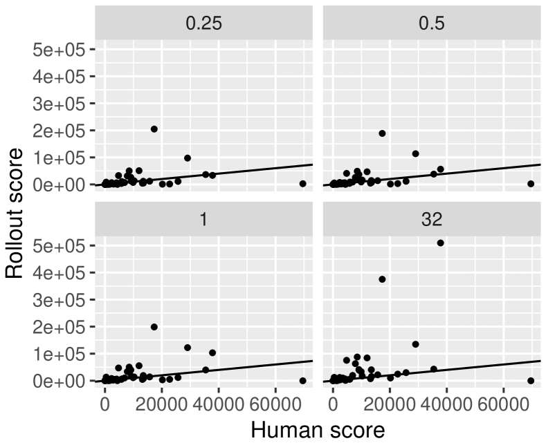
Figure 1: Scatter plots for RAS Rollout IW(1) with time budgets of 0.25, 0.50, 1, and 32 seconds vs. human playing over 49 games. Points on or above the diagonal correspond to games on which RAS Rollout IW(1) is as good as the human player.

Table 2 shows results for the human player, IW(1) using RAM, and IW(1) using the screen, and three versions of Rollout IW(1) with time budgets of 0.5 and 32 seconds. The table highlights in bold the entries that are best across each row, and in red the those that are better than human playing (except for IW(1) over RAM). Overall, for a fixed time budget, RAS Rollout IW(1) is better than RA Rollout IW(1), and this one is better than (plain) Rollout IW(1). The risk-averse versions of Rollout IW(1) are the only IW(1) algorithms that achieve a positive score for the challenging Montezuma’s Revenge, in 0.5 seconds. With 32 seconds, both RA and RAS Rollout IW(1) achieve more than 1,000 points, a good score only worse than the human player that obtains 4,367 points. Also, interestingly, IW(1) and the variants of Rollout IW(1) running over the screen states often perform better than IW(1) running until completion over the more informed RAM states.

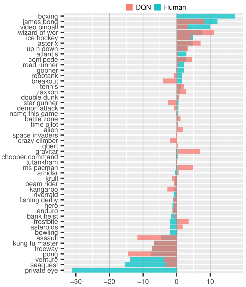
Figure 2: Comparison of RAS Rollout IW(1) with time budget of 0.5 seconds with the human player and DQN using relative scores over 48 games. Blue bars depict RAS Rollout IW(1) scores ($r)$ vs. human scores ($h$), while red bars, RAS Rollout IW(1) scores vs. DQN scores ($d$). The bar has positive length $(r-h)/h$ when $r>h$, and negative length $(h-r)/r$ when $r<h$. Bars have zero length when $r=h$. Same for $d$ in place of $h$.

Finally, Figure 2 shows a comparison of RAS Rollout IW(1) with a time budget of half a second in relation to the human player and DQN. Blue bars in the chart compare RAS Rollout IW(1) scores ($r$) and human scores ($h$), while red bars compare RAS Rollout IW(1) scores vs. DQN scores ($d$). The bar has positive length $(r-h)/h$ when $r>h$ (Rollout better), and negative length $(h-r)/r$ when $r<h$ (Human better). When $r=h=0$, the bar has zero length. Similar relations hold for $d$ in place of $h$. Games that result in infinite sized bars are excluded. This only happens for Montezuma’s Revenge as the scores for DQN and RAS Rollout IW(1) are 0 and 100 respectively.

			IW(1)		IW(1)			Rollout IW(1)			RA Rollout IW(1)			RAS Rollout IW(1)
Game		Human	RAM	x	budget .5s	budget 32s	x	budget .5s	budget 32s	x	budget .5s	budget 32s	x	budget .5s	budget 32s
alien		6,875.0	25,634.0		1,316.0	14,010.0		4,238.0	6,896.0		7,170.0	13,454.0		8,550.0	19,354.0
amidar		1,676.0	1,377.0		48.0	1,043.2		659.8	1,698.6		1,049.2	1,794.0		1,161.0	1,609.0
assault		1,496.0	953.0		268.8	336.0		285.6	319.2		336.0	327.6		264.6	281.4
asterix		8,503.0	153,400.0		1,350.0	262,500.0		45,780.0	66,100.0		46,100.0	67,100.0		48,700.0	87,600.0
asteroids		13,157.0	51,338.0		840.0	7,630.0		4,344.0	7,258.0		4,698.0	6,836.0		4,486.0	7,344.0
atlantis		29,028.0	159,420.0		33,160.0	82,060.0		64,200.0	151,120.0		122,220.0	134,660.0		113,460.0	134,660.0
bank heist		734.4	717.0		24.0	739.0		272.0	865.0		242.0	1,323.4		268.0	2,179.0
battle zone		37,800.0	11,600.0		6,800.0	14,800.0		39,600.0	414,000.0		74,600.0	455,800.0		56,200.0	509,400.0
beam rider		5,775.0	9,108.0		715.2	1,530.4		2,188.0	2,464.8		2,552.8	5,367.2		3,729.2	4,921.2
berzerk		n/a	2,096.0		280.0	1,318.0		644.0	862.0		1,208.0	1,454.0		966.0	1,640.0
bowling		154.8	69.0		30.6	49.2		47.6	45.8		44.2	49.0		51.6	48.0
boxing		4.3	100.0		99.4	79.0		75.4	79.4		99.2	100.0		78.6	80.2
breakout		31.8	384.0		1.6	56.0		82.4	36.0		86.2	336.4		79.8	370.0
centipede		11,963.0	99,207.0		88,890.0	143,275.4		36,980.2	65,162.6		56,328.0	92,353.0		46,661.4	84,226.0
chopper command		9,882.0	10,980.0		1,760.0	1,800.0		2,920.0	5,800.0		9,820.0	11,240.0		8,900.0	33,220.0
crazy climber		35,411.0	36,160.0		16,780.0	44,340.0		39,220.0	43,960.0		40,440.0	38,460.0		38,120.0	42,720.0
defender		n/a	n/a		362,010.0	430,010.0		373,010.0	256,010.0		371,010.0	374,010.0		298,010.0	387,010.0
demon attack		3,401.0	20,116.0		106.0	23,619.0		2,780.0	9,996.0		6,958.0	10,753.0		5,201.0	9,898.0
double dunk		-15.5	-14.0		-22.0	-22.4		3.6	20.0		3.2	19.6		-4.0	16.0
elevator action		n/a	13,480.0		1,080.0	0.0		0.0	0.0		0.0	0.0		0.0	1,300.0
enduro		309.6	500.0		2.6	229.2		169.4	359.4		145.8	381.0		137.4	330.8
fishing derby		5.5	30.0		-83.8	-39.0		-68.0	-16.2		-77.0	-50.2		-61.8	-53.0
freeway		29.6	31.0		0.6	25.0		2.8	12.6		2.0	11.2		3.6	10.0
frostbite		4,335.0	902.0		106.0	182.0		220.0	5,484.0		146.0	6,398.0		1,494.0	5,970.0
gopher		2,321.0	18,256.0		1,036.0	18,472.0		7,216.0	13,176.0		8,388.0	13,144.0		7,256.0	11,840.0
gravitar		2,672.0	3,920.0		380.0	1,630.0		1,630.0	3,700.0		1,660.0	5,130.0		2,410.0	5,540.0
hero		25,673.0	12,985.0		2,034.0	7,432.0		13,709.0	28,260.0		11,377.0	24,072.0		11,480.0	29,708.0
ice hockey		0.9	55.0		-13.6	-7.0		-6.0	6.6		-12.4	-2.6		5.2	18.2
james bond		406.7	23,070.0		40.0	180.0		450.0	22,250.0		10,760.0	12,656.0		5,340.0	12,345.0
kaboom		n/a	n/a		127.0	178.2		87.4	159.6		23.2	151.6		39.8	255.6
kangaroo		3,035.0	8,760.0		160.0	3,820.0		1,080.0	5,780.0		1,880.0	4,600.0		1,800.0	5,280.0
krull		2,395.0	6,030.0		3,206.8	5,611.8		1,892.8	1,151.2		2,091.8	2,219.8		1,645.2	2,837.0
kung fu master		22,736.0	63,780.0		440.0	8,980.0		2,080.0	14,920.0		2,620.0	26,540.0		2,980.0	24,300.0
montezuma’s revenge		4,367.0	0.0		0.0	0.0		0.0	0.0		100.0	1,620.0		100.0	1,080.0
ms pacman		15,693.0	21,695.0		2,578.0	20,622.8		9,178.4	19,667.0		15,115.0	23,033.0		13,746.8	21,833.0
name this game		4,076.0	9,354.0		7,070.0	13,478.0		6,226.0	5,980.0		6,558.0	6,870.0		6,128.0	6,820.0
phoenix		n/a	n/a		1,266.0	5,550.0		5,750.0	7,636.0		6,790.0	7,460.0		5,386.0	7,570.0
pitfall		n/a	n/a		-8.6	-92.2		-81.4	-130.8		-302.8	-723.4		-814.6	-692.4
pong		9.3	21.0		-20.8	0.8		-7.4	17.6		-4.2	15.2		-1.4	18.2
private eye		69,571.0	-99.0		2,690.8	-526.4		-322.0	3,157.2		-480.0	-300.0		2,160.0	-340.0
qbert		13,455.0	3,705.0		515.0	16,505.0		3,375.0	8,390.0		15,970.0	26,875.0		14,160.0	40,350.0
riverraid		13,513.0	5,694.0		664.0	7,042.0		6,088.0	8,156.0		6,288.0	14,700.0		7,138.0	15,302.0
road runner		7,845.0	94,940.0		200.0	0.0		2,360.0	37,080.0		31,140.0	44,020.0		25,780.0	62,960.0
robotank		11.9	68.0		3.2	32.8		31.0	52.6		31.2	47.4		30.0	51.8
seaquest		20,182.0	14,272.0		168.0	356.0		980.0	10,932.0		2,312.0	13,472.0		1,236.0	9,846.0
skiing		n/a	n/a		-16,511.0	-15,962.0		-15,738.8	-16,477.0		-16,006.8	-15,244.2		-15,806.6	-15,473.6
solaris		n/a	n/a		1,356.0	2,300.0		700.0	1,040.0		1,704.0	692.0		1,620.0	1,728.0
space invaders		1,652.0	2,877.0		280.0	1,963.0		2,628.0	1,980.0		1,149.0	2,533.0		1,812.0	4,362.0
star gunner		10,250.0	1,540.0		840.0	1,340.0		13,360.0	15,640.0		14,900.0	16,460.0		15,960.0	17,160.0
tennis		-8.9	24.0		-23.4	-22.2		-18.6	-2.2		-5.4	14.8		3.2	-3.4
time pilot		5,925.0	35,000.0		2,360.0	5,740.0		7,640.0	8,140.0		3,540.0	5,480.0		8,540.0	5,480.0
tutankham		167.7	172.0		71.2	172.4		128.4	184.0		135.6	191.6		147.4	191.2
up n down		9,082.0	110,036.0		928.0	62,378.0		36,236.0	44,306.0		34,668.0	39,964.0		36,936.0	41,056.0
venture		1,188.0	1,200.0		0.0	240.0		0.0	80.0		60.0	500.0		80.0	120.0
video pinball		17,298.0	388,712.0		28,706.4	441,094.2		203,765.4	382,294.8		216,468.6	378,815.4		188,604.4	375,073.0
wizard of wor		4,757.0	121,060.0		5,660.0	115,980.0		37,220.0	73,820.0		43,860.0	84,660.0		40,780.0	75,380.0
yars revenge		n/a	n/a		6,352.6	10,808.2		5,225.4	9,866.4		7,848.8	23,261.8		3,647.8	10,523.6
zaxxon		9,173.0	29,240.0		0.0	15,080.0		9,280.0	22,880.0		15,500.0	34,180.0		18,700.0	38,700.0
# $\geq$ Human		n/a	n/a		7 (14.2%)	22 (44.8%)		19 (38.7%)	34 (69.3%)		22 (44.8%)	35 (71.4%)		25 (51.0%)	37 (75.5%)
# $\geq$ 75% Human		n/a	n/a		7 (14.2%)	24 (48.9%)		22 (44.8%)	34 (69.3%)		26 (53.0%)	39 (79.5%)		29 (59.1%)	40 (81.6%)
# best in game		5 (8.6%)	24 (41.3%)		1 (1.7%)	9 (15.5%)		0 (0.0%)	2 (3.4%)		0 (0.0%)	7 (12.0%)		0 (0.0%)	11 (18.9%)

Table 2: Scores over 58 games for Human, IW(1) over RAM, and IW(1) and three versions of Rollout IW(1) with time budgets of 0.5 and 32 seconds. Entries marked as n/a are not available, those highlighted in bold are best scores across rows, and those highlighted in red are scores as good as human playing (except for IW(1) over RAM). The 9 games for which there are no reports for the human player are not considered when comparing the different algorithms with the human player.

Discussion

We have introduced a new width-based search algorithm, Rollout IW($k$), whose theoretical properties are similar to the ones for IW($k$), and have shown that it plays Atari games from the screen pixels, almost in real-time at the level of humans and some of the best reinforcement learning algorithms. These are the first results for planning in the Atari games from the screen, and they make use of the B-PROST set of visual features defined in (?). Interestingly, the results compare favorably with those obtained by planning over the memory states in many games as well. More recent RL algorithms for the ALE environment are reviewed and combined in (?), while recent work concerned with planning with images is reported in (?).

Two key differences between the proposed planning approach and reinforcement learning methods is that the latter can deal naturally with stochastic actions and result in closed-loop controllers that do not require any lookahead. One challenge for the future is to extend width-based methods such as IW(1) and Rollout IW(1) to stochastic settings, such as the “noisy” version of the Atari games supported in the latest ALE release (?). A second challenge is to use planners to obtain closed-loop policies that do not require any lookahead. One approach to do this is through imitation learning with the planner playing the role of the teacher. A more sophisticated iterated approach, akin to a pointwise version of approximate policy iteration, has been recently used in the Alpha Go Zero program that learns to play Go at superhuman level, from self-play alone, using a MCTS planner (?). Another theme for future work is the study of alternative sets of general visual features and how they relate to the theoretical width of games and the performance of the algorithms.

Acknowledgements: We thank the ALE team at the University of Alberta for the challenge and the software environment, Guillem Francès for helping Wilmer get started in this project, and Nir Lipovetzky for useful comments. H. Geffner is partially funded by grant TIN-2015-67959-P, MINECO, Spain.

References

- [Asai and Fukunaga 2017] Asai, M., and Fukunaga, A. 2017. Classical planning in deep latent space: Bridging the subsymbolic-symbolic boundary. arXiv preprint arXiv:1705.00154.
- [Bellemare et al. 2013] Bellemare, M. G.; Naddaf, Y.; Veness, J.; and Bowling, M. 2013. The arcade learning environment: An evaluation platform for general agents. Journal of Artificial Intelligence Research 47(47):253–279.
- [Ferrer-Mestres, Francès, and Geffner 2017] Ferrer-Mestres, J.; Francès, G.; and Geffner, H. 2017. Combined task and motion planning as classical AI planning. arXiv preprint arXiv:1706.06927.
- [Francès et al. 2017] Francès, G.; Ramírez, M.; Lipovetzky, N.; and Geffner, H. 2017. Purely declarative action representations are overrated: Classical planning with simulators. In Proc. IJCAI.
- [Geffner and Geffner 2017] Geffner, T., and Geffner, H. 2017. Width-based planning for general video-game playing. In Proc. AIIDE.
- [Hessel et al. 2017] Hessel, M.; Modayil, J.; Van Hasselt, H.; Schaul, T.; Ostrovski, G.; Dabney, W.; Horgan, D.; Piot, B.; Azar, M.; and Silver, D. 2017. Rainbow: Combining improvements in deep reinforcement learning. arXiv preprint arXiv:1710.02298.
- [Kocsis and Szepesvári 2006] Kocsis, L., and Szepesvári, C. 2006. Bandit based Monte-Carlo planning. In Proc. ECML-2006, 282–293. Springer.
- [Liang et al. 2016] Liang, Y.; Machado, M.; Talvitie, E.; and Bowling, M. 2016. State of the art control of Atari games using shallow reinforcement learning. In Proc. of the 2016 Int. Conf. on Autonomous Agents & Multiagent Systems (AAMAS), 485–493.
- [Lipovetzky and Geffner 2012] Lipovetzky, N., and Geffner, H. 2012. Width and serialization of classical planning problems. In Proc. ECAI, 540–545.
- [Lipovetzky and Geffner 2017] Lipovetzky, N., and Geffner, H. 2017. Best-first width search: Exploration and exploitation in classical planning. In Proc. AAAI, 3590–3596.
- [Lipovetzky, Ramírez, and Geffner 2015] Lipovetzky, N.; Ramírez, M.; and Geffner, H. 2015. Classical planning with simulators: Results on the Atari video games. In Proc. IJCAI, 1610–1616.
- [Machado et al. 2017] Machado, M.; Bellemare, M. G.; Talvitie, E.; Veness, J.; Hausknecht, M.; and Bowling, M. 2017. Revisiting the arcade learning environment: Evaluation protocols and open problems for general agents. arXiv preprint arXiv:1709.06009.
- [Mnih et al. 2015] Mnih, V.; Kavukcuoglu, K.; Silver, D.; Rusu, A.; Veness, J.; Bellemare, M. G.; Graves, A.; Riedmiller, M.; Fidjeland, A.; Ostrovski, G.; et al. 2015. Human-level control through deep reinforcement learning. Nature 518(7540):529–533.
- [Shleyfman, Tuisov, and Domshlak 2016] Shleyfman, A.; Tuisov, A.; and Domshlak, C. 2016. Blind search for Atari-like online planning revisited. In Proc. IJCAI, 3251–3257.
- [Silver et al. 2017] Silver, D.; Schrittwieser, J.; Simonyan, K.; Antonoglou, I.; Huang, A.; Guez, A.; Hubert, T.; Baker, L.; Lai, M.; Bolton, A.; et al. 2017. Mastering the game of go without human knowledge. Nature 550(7676):354–359.