Study of Active Brownian Particle Diffusion in Polymer Solutions

Abstract

The diffusion behavior of an active Brownian particle (ABP) in polymer solutions is studied using Langevin dynamics simulations. We find that the long time diffusion coefficient $D$ can show a non-monotonic dependence on the particle size $R$ if the active force $F_{a}$ is large enough, wherein a bigger particle would diffuse faster than a smaller one which is quite counterintuitive. By analyzing the short time dynamics in comparison to the passive one, we find that such non-trivial dependence results from the competition between persistence motion of the ABP and the length-scale dependent effective viscosity that the particle experienced in the polymer solution. We have also introduced an effective viscosity $\eta_{\text{eff}}$ experienced by the ABP phenomenologically. Such an active $\eta_{\text{eff}}$ is found to be larger than a passive one and strongly depends on $R$ and $F_{a}$. In addition, we find that the dependence of $D$ on propelling force $F_{a}$ presents a well scaling form at a fixed $R$ and the scaling factor changes non-monotonically with $R$. Such results demonstrate that active issue plays rather subtle roles on the diffusion of nano-particle in complex solutions.

I INTRODUCTION

Transport properties of macromolecule are of great importance in various fields including biophysics(Wang et al., 2012; Sigalov, 2010; Pederson, 2000; Cluzel et al., 2000), material (Struntz and Weiss, 2015; Gersappe, 2002; Zhou et al., 2007; Shah et al., 2005), medicine(Rohilla et al., 2016; Huo et al., 2014), and so on. One of the research interests in recent years is the diffusion of macromolecule (protein or nano-particle) in complex solution systems. Especially in living cells, a variety of structural and functional proteins are immersed in crowded cytoplasmic environments, involved in diverse biochemical processes such as enzyme reactions(Berry, 2002), signal transmission(Wang et al., 2012), gene transcription and self-assembly of supramolecular(Macnab, 2000). Experimentally, one would usually focus on nano-particle (NP) in complex environment such as polymer solution. And study of diffusive behavior of NP can provide important information about the local structure , viscoelastic properties and also the crowding effect of polymer liquids(Lu and Solomon, 2002; Waigh, 2005; Cicuta and Donald, 2007).

In the past decades, diffusion of NPs in polymer solutions has received a lot of attention both experimentally (Kohli and Mukhopadhyay, 2012a; Chen et al., 2016; Pryamitsyn and Ganesan, 2016a; Lee et al., 2017; Poling-Skutvik et al., 2015) and theoretically (Tuinier and Fan, 2008a; Ganesan et al., 2006; Yamamoto and Schweizer, 2014; Dong et al., 2015; Feng et al., 2016; Egorov, 2011; Yamamoto and Schweizer, 2011). In experiments, fluctuation correlation spectroscopy (FCS) (Omari et al., 2009; Holyst et al., 2009a; Michelman-Ribeiro et al., 2007; Grabowski et al., 2009), dynamic light scattering (DLS) (Holyst et al., 2009a; Koenderink et al., 2004), and capillary viscosimetry are general tools to investigate the diffusion of a NP in complex fluids. It is found that as the particle radius $R$ decreases to nanoscale, the diffusion coefficient $D$ would increase exponentially with $R$ and violates the Stokes-Einstein (SE) relation apparently(Ye et al., 1998; Schachman and Harrington, 1952; Tuteja et al., 2007; Kohli and Mukhopadhyay, 2012b; Wang et al., 2010). Phillies $et$ $al$, based on the analysis of a great deal of experimental data, proposed an empirical formula $D=D_{0}\exp(-\alpha c^{v})$, where $D_{0}$ is the diffusion coefficient in a purely background solvent, $c$ is the concentration of polymer solution and $\alpha$, $v$ are fitting parameters relevant to a specific system(Phillies, 1986). Although this stretched exponential form matches the experimental data very well, the underlying physical meaning of these two parameters are quite blurry(Kalwarczyk et al., 2015). Recently, Holyst $et$. $al$ proposed a length-scale dependent viscosity theory(Holyst et al., 2009b; Kalwarczyk et al., 2011). They argued that the diffusion of a NP in polymer solution was characterized by at least three length scales: the particle size $R$, the polymer hydrodynamic radius $R_{h}$ and the correlation length $\xi$ of the solution. Concretely, the formula reads $D/D_{0}\sim\exp\left[b\left(R_{\text{eff}}/\xi\right)^{a}\right]$, where $R_{\text{eff}}=\sqrt{R^{2}R_{h}^{2}/(R^{2}+R_{h}^{2})}$ denotes an effective size, $a$ and $b$ are fitting parameters. If $R$ is small with respect to $\xi$, the particle motion experiences the local viscosity which is smaller than the macro-viscosity by order of magnitude. While if $R$ is much larger than $R_{h}$ or $R_{g}$, the particle motion would no more be affected by the local structures of polymer and touches the macro viscosity finally, and obeys the Stokes-Einstein relation automatically. Also, there are some other interesting models in this field such as the hopping model(Cai et al., 2015), walking confined diffusion model(Ochab-Marcinek and Hołyst, 2011) and depletion model(Tuinier and Fan, 2008b). Liu $et$ $al$ used a MD simulation to study the diffusion of a NP in polymer melt (Liu et al., 2008)and the core results are similar to Holyst’s work, where $R_{g}$ could be the boundary of NP size to experience the local viscosity to macro viscosity. Note that, it is hard to take a simulation work on this issue especially the polymer solution, which on one side the solvent accounts for a large proportion and costs a huge computational resource, and on other side a reasonable diffusion coefficient needs so much long time to evolve the system . To our best of knowledge, only in the recent two years, Li $et$ $al$ (Li et al., 2016; Chen et al., 2017)and Pryamitsyn $et$ $al$(Pryamitsyn and Ganesan, 2016b) had studied this issue in a simulation way, using Multiparticle Collision Dynamic (MPCD) and Dissipative Particle Dynamic (DPD) method respectively.

Most of the present works focus on the diffusion of passive NP. But note that, in real biological system, especially in a living cell, the active proteins widely exist. Typical active proteins include motor molecule(Zheng et al., 2000; Duan et al., 2016), microtubule or active filament(Sumino et al., 2012; Loose and Mitchison, 2014). By consuming the ATP, they get a propel force that extremely enhance the transport efficiency in various biochemical process. Actually, the dynamics behavior of active matter has gained much attention in recent years. Instead of the living species such as bacteria(Sokolov et al., 2007), spermatozoa(Woolley, 2003; Riedel et al., 2005) and the micro protein in cell as mentioned above, there are also much artificial objects capable of self-propulsion such as Janus particles(Howse et al., 2007), chiral particles(Ghosh and Fischer, 2009), and vesicles(Joseph et al., 2016). And a wealth of new non-equilibrium phenomena have been reported, including phase separation(Fily and Marchetti, 2012), active turbulence(Dunkel et al., 2013), and active swarming(Cohen and Golestanian, 2014), both experimentally and theoretically.

Recently, much interests arised on the dynamic behaviors of an active particle in complex environment(Shen and Arratia, 2011; Gagnon et al., 2014; Thomases and Guy, 2014; Patteson et al., 2016). And a number of studies indicated that there exists a two-way coupling between the active matter and the ambient environment, which the motion of active suspensions can alter the local property of its environment, while simultaneously the complex fluid rheology can modify the dynamics of the active matters(Patteson et al., 2016). For instance, Patteson $et$ $al$ reported an experiment on the diffusion of an Escherichia coli in polymeric solution(Patteson et al., 2015). They found that the translational diffusion of cell is enhanced and the rotational diffusion is sharply declined respected to the diffusion behavior in water-like fluid, due to the complicated interaction with the polymers in solution. It was also found that activity has a fascinating effect on the viscosity of active suspensions, even sometimes leading to a “vanishing” viscosity phenomenon in bacterial suspensions(López et al., 2015). Even for a single swimmer, there is no universal answer to whether mobility is enhanced or hindered by fluid elasticity(Patteson et al., 2016). Despite lot of interesting progresses made so far, there still remains many open questions to be answered, even some fundamental ones. For instance, how would the long time diffusion coefficient of an active particle depends on its size in a complex fluid, although being a quite straightforward question, has not been systematically studied yet.

In the present work, we have addressed such a topic by investigating the diffusion dynamics of an active Brownian particle (ABP) in polymer solutions, as depicted schematically in Fig.1. The ABP is modeled by a spherical particle subjected to an active force along the direction denoted by $\mathbf{n}$, which changes randomly with time. Three-dimensional Langevin simulations are performed to calculate the long time diffusion coefficient $D$ of the ABP as a function of the particle size $R$, for a variety of different active force $F_{a}$ as well as polymer concentration $\phi$. Very interestingly, we find that $D$ shows a non-monotonic dependence on $R$ if the active force $F_{a}$ is large enough: $D$ first increases with the particle size $R$, reaches a maximum value at an optimal particle size $R_{\text{opt}}$, after which it decreases monotonically. The optimal value $R_{\text{opt}}$ moves to a larger value with the increment of active force $F_{a}$ and to a smaller value with increasing polymer concentration. Further analysis of the time dynamics of the mean-square displacement (MSD) indicates that it is the competition between the persistence motion of the particle, which is the reason for superdiffusion, and the cage effect of the polymer solution, which leads to the subdiffusion behavior, that causes the optimal size effect for long time diffusion. We have also introduced an effective viscosity experienced by the ABP by introducing a phenomenological model describing the ABP moving in a fluid with effective viscosity $\eta_{\text{eff}}^{a}$. Such an effective viscosity is found to be larger than that experienced by a passive particle, and it shows strong dependency on the particle size $R$ as well as the active force amplitude $F_{a}$. In addition, we have found that $D$ shows a power law dependence on the active force $F_{a}$, i.e., $D\sim F_{a}^{\alpha}$, for a fixed particle size. More interestingly, the exponent $\alpha$ also shows a non-monotonic dependence on the particle size $R$: $\alpha<2.0$ for small $R$, then it increases with $R$ to a maximum value $\alpha\sim 2.5$ for an intermediate particle size, and finally approaches 2.0 in the large size limit. Our findings demonstrate that interplay between particle activity and local structure in complex solution may lead to interesting dynamics of the ABP.

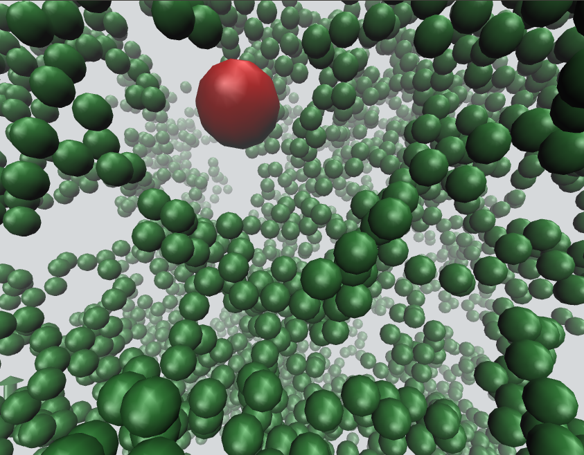
Figure 1: The illustration of a ABP immerses in polymer solution, which the big red particle represents ABP and the green particle around represents polymer bead.

The paper is organized as follows. In section II , we describe the model and simulation method. Results and discussion are presented in section III followed by conclusion in section IV .

II Simulation method

As shown in Fig.1, we consider a three dimensional system containing a single ABP of radius $R$ in polymer solution. The polymers are modeled as bead-spring chains, each consisting of $N$ beads with diameter $\sigma$. All non-bonded (excluded volume) interactions between the beads are modeled by purely repulsive Weeks-Chandler-Andersen (WCA) potentials(Weeks et al., 1971):

$$U_{\text{BB}}(r_{ij})=\begin{cases}4\epsilon\left[(\frac{\sigma}{r_{ij}})^{12}-(\frac{\sigma}{r_{ij}})^{6}+\frac{1}{4}\right]&\qquad r_{ij}<\sqrt[6]{2}\sigma\\ 0&\qquad r_{ij}\geq\sqrt[6]{2}\sigma\end{cases}$$ (1)

where $r_{ij}=\left|\mathbf{r}_{i}-\mathbf{r}_{j}\right|$ denotes the distance between the two beads $i$ and $j$ (with position vectors given by $\mathbf{r}_{i}$ and $\mathbf{r}_{j}$, respectively), $\epsilon$ represents strength of the WCA potential. The bond interaction between two nearby beads is modeled by the FENE (finite extensible nonlinear elastic) potential(Kremer and Grest, 1990):

$$U_{\text{FENE}}(r_{ij})=-\frac{1}{2}\epsilon_{F}r_{F}^{2}\ln\left[1-(\frac{r_{ij}}{r_{F}})^{2}\right]$$ (2)

where $\epsilon_{F}$ is the interaction strength and $r_{F}=2.0\sigma$ denotes the upper bound of $r_{ij}$.

The interactions between the NP and polymer beads are also described by the truncated WCA potential which is offset by the interaction range $R_{ev}=R-\sigma/2$:

$$U_{BN}(r_{jn})=4\epsilon\left[(\frac{\sigma}{r_{jn}-R_{ev}})^{12}-(\frac{\sigma}{r_{jn}-R_{ev}})^{6}+\frac{1}{4}\right]$$ (3)

for $R_{ev}<r_{jn}<R_{ev}+2^{1/6}\sigma$, where $r_{jn}$ denotes the distance between bead $j$ and the nano-particle with position given by $\mathbf{r}_{n}$. While for $r_{jn}\leq R_{ev}$, $U_{BN}(r_{jn})=\infty$ and for $r_{jn}\geq R_{ev}+2^{1/6}\sigma$, $U_{BN}(r_{jn})=0$.

The dynamics of the polymer beads are described by the following Langevin equations(ignoring hydrodynamic interactions):

$$m_{\text{B}}\frac{d^{2}\mathbf{r}_{j}}{dt^{2}}=-\gamma_{\text{B}}\frac{d\mathbf{r}_{j}}{dt}-\nabla_{\mathbf{r}_{j}}U^{\prime}+\sqrt{2k_{\text{B}}T\gamma_{\text{B}}}\bm{\xi}_{j}(t)$$ (4)

where $U^{\prime}=\sum_{i\neq j}U_{\text{BB}}\left(r_{ij}\right)+U_{\text{BN}}\left(r_{jn}\right)$ , $m_{B}$ is the bead mass and $\gamma_{B}$ is the friction coefficient of the bead in the background pure solvent, $\bm{\xi}_{j}\left(t\right)$ denotes independent Gaussian white noises with zero means and unit variances, i.e., $\left\langle\bm{\xi}_{j}\left(t\right)\right\rangle=0$, $\left\langle\bm{\xi}_{i}\left(t\right)\bm{\xi}_{j}\left(t^{\prime}\right)=2\delta_{ij}\mathbf{I}\delta\left(t-t^{\prime}\right)\right\rangle$ where $\mathbf{I}$ is the unit tensor.

The dynamics of the ABP is given by

$$m_{\text{N}}\frac{d^{2}\mathbf{r}_{n}}{dt^{2}} =-\gamma_{\text{N}}\frac{d\mathbf{r}_{n}}{dt}+F_{a}\textbf{n}-\nabla_{\mathbf{r}_{n}}\left[\sum_{j}U_{\text{BN}}\left(r_{jn}\right)\right]+\bm{\xi}_{n}(t)$$ (5)

$$\frac{d\mathbf{n}}{dt} =\bm{\eta}\left(t\right)\times\mathbf{n}$$ (6)

where $m_{N}$ is the mass of the ABP and $\gamma_{N}$ is the friction coefficient of the ABP in the pure solvent. $\mathbf{r}_{n}$ is the position vector of the ABP, $r_{jn}=\left|\mathbf{r}_{j}-\mathbf{r}_{n}\right|$ is the distance between polymer bead $j$ and the ABP. $F_{a}$ represents the amplitude of active force with orientation specified by the unit vector $\mathbf{n}$. $\bm{\xi}_{n}\left(t\right)$ is also a Gaussian white noise vector with $\left\langle\xi_{n}\left(t\right)=0\right\rangle$ and $\left\langle\bm{\xi}_{n}\left(t\right)\bm{\xi}_{n}\left(t^{\prime}\right)\right\rangle=2D_{t}\mathbf{I}\delta\left(t-t^{\prime}\right)$, where $D_{t}=k_{B}T/\gamma_{N}$ is the (short time) translational diffusion coefficient. The stochastic vector $\bm{\eta}\left(t\right)$ is also Gaussian distributed with zero mean and has time correlations given by $\left\langle\bm{\eta}\left(t\right)\bm{\eta}\left(t^{\prime}\right)\right\rangle=2D_{r}\mathbf{I}\delta\left(t-t^{\prime}\right)$, where $D_{r}$ denotes the rotational diffusion coefficient. Since we consider a spherical particle here, $D_{t}$ is related to $D_{r}$ via $D_{r}=3D_{t}/\left(2R\right)^{2}$.

All simulations were performed in a cubic box with a $25\sigma$ edge length with periodic boundary conditions in all directions. A value $\epsilon=k_{B}T$ was used for all particle interactions, where $k_{\text{B}}$ is Boltzmann’s constant and $T$ temperature. The polymers were modeled using $N=64$ beads and the parameters for bond-interactions are $k_{\text{F}}=10k_{\text{B}}T\sigma^{-2}$ and $r_{\text{F}}=2.0\sigma$. If not otherwise specified, we considered a system containing 72 polymer chains, corresponding to a bead-number concentration $\phi\simeq 0.3$. For other polymer concentrations, we simply varied the number of polymer chains. We assumed equal densities of the ABP and polymer bead, thus $m_{\text{N}}=8R^{3}/\sigma^{3}$$m_{\text{B}}$. Since the friction coefficient $\gamma$ is proportional to $6\pi\eta_{0}R$ for a spherical particle of radius $R$ in the pure solvent, where $\eta_{0}$ is the zero-shear viscosity of the pure solvent, we have $\gamma_{\text{N}}=\left(2R/\sigma\right)\gamma_{\text{B}}$. We set $m_{\text{B}}=1$, $k_{\text{B}}T=1$, $\sigma=1$ for dimensionless units and then fixed $\gamma_{\text{B}}=1$. The remained variable parameters are the active force amplitude $F_{a}$ and the particle radius $R$. Velocity-Verlet algorithm was used to simulate the dynamic equations with a time step $\Delta t=0.01$. All the reported data below were obtained after averaging over 20 independent runs with long enough time.

III Results And Discussion

III.1 Optimal Size for Active Particle Diffusion

In the present paper, we are mainly interested in how the activity would influence the NP diffusion behavior in the polymer solution. For comparison, we first investigate the diffusion behavior of a passive particle in the system set above. The long time diffusion coefficient $D$ is calculated via

$$D=\lim\limits_{t\to\infty}\frac{1}{6t}\langle\Delta r_{n}^{2}(t)\rangle$$

where $\langle\Delta r_{n}^{2}(t)\rangle=\langle|\textbf{r}_{n}(t)-\textbf{r}_{n}(0)|^{2}\rangle$ is the mean square displacement (MSD) of the NP with $\textbf{r}_{n}(t)$ being the particle position at time $t$. As already mentioned in the introduction section, passive particle diffusion in polymer solutions may strongly deviates the SE relation. In particular, the diffusion coefficient $D$ can be described by scaling relations involving the correlation length of the polymer solution and an effective size. Note that the system parameters used in our present work may not fit well the experimental conditions. In Fig.2(a), the diffusion coefficients $D$ of a passive NP as functions of the radius $R$ for several fixed values of polymer concentration $\phi=0.1,\>0.2\text{ and }0.3$ are presented. Clearly, $D$ decreases monotonically with increasing of $R$ as well as the polymer concentration $\phi$ as expected. We can introduce an effective (so-called) nano-viscosity $\eta_{\text{eff}}$ experienced by the NP via the standard SE relation $D=k_{B}T/6\pi\eta_{\text{eff}}R$. In the large particle size limit, $\eta_{\text{eff}}$ would be the macroscopic zero-shear viscosity $\eta_{macro}$ of the polymer solution. For small particle size, however, $\eta_{\text{eff}}$ is much smaller than $\eta_{macro}$ leading to large deviations from the SE relation. In Fig.2(b), the nano-viscosity as a function of the NP size $R$ is shown for different concentration $\phi$. $\eta_{\text{eff}}$ firstly increases fiercely with $R$ until it finally reaches the macroscopic value $\eta_{macro}$ for large particle sizes. It suffices to reach $\eta_{macro}$ for a NP with size to be just a few times of that of a polymer bead and NP in a more concentrated polymer solution can reach $\eta_{macro}$ at a smaller $R$.

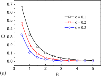
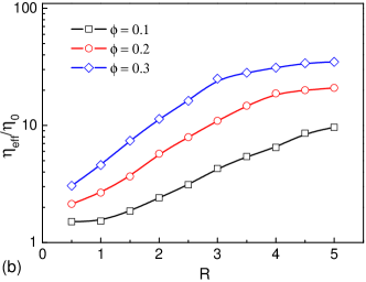
Figure 2: The diffusion coefficient $D$ (a) and the effective viscosity $\eta_{\text{eff}}$ (b) of a passive NP with respect to different size $R$, under the concentration of polymer $\phi=0.1,$ 0.2 and 0.3, respectively. Note that $\eta_{\text{eff}}$ is reduced by the viscosity of pure solution $\eta_{0}$. The solid lines are drawn to guide the eyes.

We now turn to the ABP. In Fig.3(a), $D$ as a function of $R$ at a fixed concentration $\phi=0.3$ is presented, for a few different values of propelling force $F_{a}$. For a relatively small active force, e.g., $F_{a}=20$ as shown in black line in Fig.3(a), $D$ decreases monotonically with the particle size $R$, which is similar to the case of a passive particle as shown in Fig.2. For larger active forces, however, $D$ shows an interesting non-monotonic dependence on the particle size $R$, i.e., $D$ first increases with $R$ until it reaches a maximum value $D_{max}$ at an optimal size $R_{opt}$ and then decreases again, as demonstrated clearly in Fig.3(a) for $F_{a}=40,\,60,$ and 80, respectively. With increasing $F_{a}$, the overall values of $D$ become larger and the optimal size slightly $R_{opt}$ shifts to larger values. In Fig.3(b), dependence of the optimal particle size $R_{opt}$ on the active force $F_{a}$ for a few different polymer concentrations $\phi$ are depicted. For a fixed $\phi$, $R_{opt}$ increases with $F_{a}$ as already shown in Fig.3(a), while $R_{opt}$ decreases with $\phi$ if $F_{a}$ is fixed.

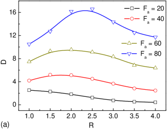
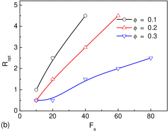
Figure 3: (a) The diffusion coefficient $D$ of ABP as a function of the particle radius $R$, for difference active forces $F_{a}=20,$ 40, 60 and 80 and fixed $\phi=0.3$. (b) Dependence of $R_{\text{opt}}$ on active force $F_{a}$ for different number concentrations $\phi=0.1$, 0.2 and 0.3. The solid lines are drawn to guide the eyes.

The above findings about the non-monotonic dependence of $D$ on $R$ is quite counterintuitive at the first glance, particularly in terms of the increasing of $D$ with $R$. Generally, one would expect that a larger particle would diffuse more slowly as the conventional SE relation would tell. For a passive nano-particle in a polymer solution, although large deviations from the SE relation were observed and a length-scale viscosity should be used in replace of the macroscopic viscosity $\eta_{macro}$, $D$ is always a decreasing function of $R$ as already shown in Fig.2. Therefore, the increase of $D$ with $R$ as shown in Fig.3(a) must be related to the active feature of the ABP. Indeed, if the active force is not large enough, as shown for $F_{a}=20$ in Fig.3(a), $D$ will still be a decreasing function of $R$, being same to the case of a passive NP. For large active force, the non-monotonic dependence of $D$ on $R$ suggests the existence of two competitive factors that influence the ABP diffusion.

III.2 Subdiffusion and Superdiffusion

In order to understand in more detail about such nontrivial dependence of $D$ on $R$, we further analyze the short time dynamics of the ABP by investigating the MSD as a function of time $t$, and compare it to that of a passive one.

Fig.4(a) presents the MSDs for passive NPs with radius $R=1$, 2 and 4 for $\phi=0.3$. The curves share some common features, namely, ballistic diffusion at very short time while normal diffusion at very long time, correspond to $\text{MSD}\sim t^{2}$ and $\text{MSD}\sim t$ respectively. For a small NP, such as $R=1.0$, the dynamics transformers from ballistic motion to normal diffusion gradually. With increasing particle size, the NP may experience a “cage effect” resulting from the surrounding polymer beads and the MSD shows a sub-diffusion regime at the middle time scale, wherein $\text{MSD}\sim t^{\alpha}$ with $\alpha<1$. This is shown more clearly in Fig.5(a), where the instantaneous exponent $\alpha$ is depicted as a function of time corresponding to Fig.4(a). Obviously, with increasing the NP size, the cage effect is more remarkable and $\alpha$ decreases to a smaller value in the intermediate time scale, corresponding to a stronger and longer subdiffusion behavior. Also note that the curve for a larger particle always lies below that for a smaller one in the whole time range.

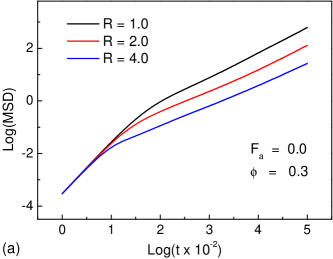
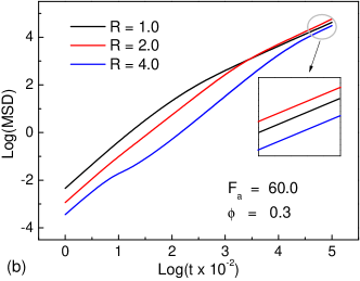
Figure 4: MSD of an active NP (a) and a passive NP (b) with size $R=1.0$, 2.0, 4.0. The short line indicates the time scaling at different time scale. For an active NP, the magnitude of propelling force is fixed at $F_{a}=20.0$.

For an ABP, however, the behavior is quite different, as shown in Fig.4(b) and Fig.5(b) for $F_{a}=60$. For this large active force, the diffusion coefficient $D$ shows non-monotonic dependence on $R$ as demonstrated in last subsection. For a small particle with $R=1.0$, the behavior shows no distinct difference from that of a passive one in terms of both the MSD curve as well as the exponent $\alpha$. For a larger particle with $R=2.0$, however, we find that the particle undergoes a much longer superdiffusion time regime with $1<\alpha<2$ before it finally reaches the long time normal diffusion regime. Interestingly, the exponent $\alpha$ shows an apparent plateau at $\alpha\sim 1.7$ as shown in Fig.5(b) which spans two orders of magnitude of time. Such a superdiffusion behavior with $\alpha$ slightly smaller than 2 implicates that the particle moves more persistently along a direction than randomly along different directions. Note that this persistence of motion along a direction reflects the very feature of an active Brownian particle. For an even larger particle $R=4.0$, one can see that the exponent $\alpha$ first decreases sharply to a value at 0.9 in the short time range, namely indicated a sub-diffusion behavior, and then increases again to a high value close to 2 in the intermediate range before it finally decreases to the normal diffusion value $\alpha=1$. The sharp decrease of $\alpha$ in the short time range should result from the cage effect of the surrounding polymers. Due to the large activity of the particle, however, such a cage effect can not last for a long time and finally the particle jumps out of this cage leading to the increase of $\alpha$ in the intermediate time range. In the short time range, ABP with a smaller size moves faster than a larger one as shown in Fig.4(b). However, in the long time limit, the curve for a middle particle size $R=2$ lies above those of $R=1$ and 4, corresponding to a maximum value of long time diffusion coefficient $D$ for $R=2$ compared to those others two in accordance with Fig.3.

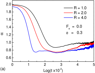
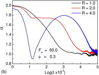
Figure 5: The differential of MSD of of a passive NP (a) and an ABP (b) with size R = 1.0, 2.0 and 4.0 in the polymer solution with concentration $\phi=0.3$ . $\alpha$ is just the slope of curve in Fig.4 or the scaling exponent at different time scale. For an ABP depicted in (b) , the magnitude of propelling force is fixed at $F_{a}=60.0$.

The above analysis suggests that the occurrence of an optimal particle size for ABP diffusion in polymer solution is the consequence of two competitive effects. One is that the cage effect of the surrounding polymers which would become stronger as the particle size becomes larger. Without activity, this cage effect would lead to subdiffusion behavior of a particle and decrease of the long time diffusion coefficient $D$. Such a cage effect results in a length-scale dependent viscosity experienced by the particle as described in Fig.2(b) which increases with $R$. The other is the persistence motion due to the particle activity which would become longer as the particle size increases. As well known for an ABP and described in the model section, the persistence time $\tau_{p}$ for an isolated ABP is given by $\left(2D_{r}\right)^{-1}$, where $D_{r}$ scales as $R^{-2}$ for the ABP as shown in section II. Therefore, the ABP would move along the propelled direction longer as the particle size gets larger, leading to superdiffusive behavior and thus accelerating the long time diffusion. When the particle size is small, e.g. $R=1$, both cage and persistence effects are not significant and the particle transfers gradually from ballistic to diffusion motion for both passive and active particles. For a relatively larger particle, the persistence effect would dominate, thus leading to increase of $D$. If the particle size is too large, however, the cage effect would dominate and the diffusion coefficient would decrease again. Besides, increasing the magnitude of $F_{a}$, the persistence motion would be enhanced. Clearly, this enhancement will be more apparent for a bigger ABP with longer $\tau_{p}$. Therefore, the stronger $F_{a}$ promotes $R_{opt}$ to a bigger value as shown in Fig.3(b).

III.3 Effective Viscosity $\eta_{\text{eff}}$

As discussed in Section 3.1, a passive particle would experience an effective viscosity $\eta_{\text{eff}}$ that is dependent on its size $R$, which could be much smaller than the macroscopic zero-shear viscosity $\eta_{\text{macro}}$. For a passive particle, this effective viscosity is determined according to the SE relation, $D=k_{\text{B}}T/\left(6\pi\eta_{\text{eff}}R\right)$. It is thus also interesting for us to ask the question what is the effective viscosity the ABP experiences in the polymer solution.

At first thought, one may also just use the SE relation to obtain this effective viscosity $\eta_{\text{eff}}$, i.e., $\eta_{\text{eff}}=k_{\text{B}}T/\left(6\pi DR\right)$ where $D$ is the long time translational diffusion coefficient obtained by simulation above. Nevertheless, this may not be appropriate for an active particle, since we must take into account the particle activity which would lead to an active contribution to $D$. As already discussed in the model section, for an isolated ABP of radius $R$ in a simple fluid with friction coefficient $\gamma$, the dynamics can be described by the following overdamped Langevin equation (LE),

$$\frac{d\mathbf{r}}{dt} =\gamma^{-1}F_{a}\textbf{n}+\sqrt{2D_{t}}\mathbf{\bm{\xi}}\left(t\right)$$ (7)

$$\frac{d\mathbf{n}}{dt} =\bm{\zeta}\left(t\right)\times\mathbf{n}$$

where $\bm{\xi}\left(t\right)$ and $\bm{\zeta}\left(t\right)$ are both Gaussian white noise vectors with zero mean and unit(tensor) variance, $D_{t}=k_{B}T/\gamma$ and $D_{r}=3D_{t}/4R^{2}$. In a coarse-grained time scale, it was shown that the self-propulsion force for ABP can be mapped into a colored noise(Bechinger et al., 2016), i.e.,

$$\left\langle\mathbf{n}\left(t\right)\mathbf{n}\left(t^{\prime}\right)\right\rangle\simeq\frac{1}{3}e^{-\left|t-t^{\prime}\right|/\tau_{p}}\mathbf{1}$$

where $\mathbf{1}$ denotes the unit tensor and $\tau_{p}=\left(2D_{r}\right)^{-1}$ denotes the persistence time of the self-propulsion force. With this approximation, one can obtain the mean-square displacement (MSD) of the ABP as follows,

$$\left\langle\delta r^{2}\left(t\right)\right\rangle=\frac{2F_{a}^{2}\tau_{p}}{\gamma^{2}}\left[t+\tau_{p}\left(e^{-t/\tau_{p}}-1\right)\right]+6D_{t}t$$

In the long time limit, this gives the diffusion coefficient

$$D=\lim_{t\to\infty}\frac{1}{6}\frac{\left\langle\delta r^{2}\left(t\right)\right\rangle}{t}=D_{t}+\frac{F_{a}^{2}\tau_{p}}{3\gamma^{2}}$$

If we use the fact that $\tau_{p}=\left(2D_{r}\right)^{-1}$ and $D_{r}=3D_{t}/4R^{2}$, then we have

$$D=\frac{k_{B}T}{\gamma}+\frac{2F_{a}^{2}R^{2}}{9k_{B}T\gamma}=\frac{1}{6\pi\eta_{0}R}\left(k_{\text{B}}T+\frac{2F_{a}^{2}R^{2}}{9k_{\text{B}}T}\right)$$ (8)

where we have used the Stokes relation $\gamma=6\pi\eta_{0}R$ in the simple fluid with $\eta_{0}$ the zero-shear viscosity. This analysis shows how the long time diffusion coefficient $D$ depends on the viscosity $\eta_{0}$ of a simple fluid. The first term is surely the SE relation, while the second term denotes the contribution from particle activity. For small $T$ or large $F_{a}$, the second active term would dominate and the relation between $D$ and $\eta_{0}$ is totally different from the SE relation.

Actually, eqn (8) provides us a scheme to introduce an effective viscosity experienced by the ABP in the surrounding solution. We consider now that the ABP is moving in a pure fluid with effective viscosity $\eta_{\text{eff}}$, whose dynamics is also described by eqn (7), but with $\gamma$ replaced by an effective $\gamma_{\text{eff}}^{a}=6\pi\eta_{\text{eff}}^{a}R$ (the superscript ‘a’ stands for ‘active’). The (short time) translational diffusion constant $D_{t}$ is determined then by $\gamma_{\text{eff}}^{a}$ through fluctuation-dissipation theorem $D_{t}=k_{\text{B}}T/\gamma_{\text{eff}}^{a}$, which in turn gives $D_{r}$. Clearly, the long time diffusion coefficient $D$ would also be given by eqn (8) with $\eta_{0}$ replaced by $\eta_{\text{eff}}^{a}$, i.e.,

$$D=\frac{1}{6\pi\eta_{\text{eff}}^{a}R}\left(k_{\text{B}}T+\frac{2F_{a}^{2}R^{2}}{9k_{\text{B}}T}\right)$$ (9)

Therefore, the effective viscosity of the polymer solution experienced by the ABP could be defined as

$$\eta_{\text{eff}}^{a}=\frac{1}{6\pi DR}\left(k_{\text{B}}T+\frac{2F_{a}^{2}R^{2}}{9k_{\text{B}}T}\right)$$ (10)

In Fig.6(a), we show the effective viscosity $\eta_{\text{eff}}^{a}$ calculated by eqn (10) as functions of the particle size $R$ for different concentrations $\phi=0.1$, 0.2 and 0.3, where the values of $D$ are obtained by simulations as shown in Fig.3. The amplitude of the active force is $F_{a}=20$. Also shown are the values for a passive particle, which were already presented in Fig.2(b). As can be seen, $\eta_{\text{eff}}^{a}$ increases with $R$ as expected, similar to the case of $\eta_{\text{eff}}$ for a passive particle. Interestingly, $\eta_{\text{eff}}^{a}$ is much larger than $\eta_{\text{eff}}$ as shown in Fig.6(a), indicating that the active particle seems to move in a “more viscous” fluid than the passive one. Nevertheless, one should be careful to draw the conclusion that particle activity induces thickening of the polymer solution, since $\eta_{\text{eff}}^{a}$ here is defined via eqn (6). As discussed above, this equation is obtained by modeling the motion of ABP in polymer solution as if it were in an viscous fluid with $\eta_{\text{eff}}^{a}$, while keeping fluctuation-dissipation theorem and all other features of ABP unchanged. Indeed, the effective viscosity experienced by an ABP characterize more the local environment surrounding the particle, and it is not identical to the zero-shear macro-viscosity of the solution. Our arguments here indicate that the ABP does feel a much more viscoelastic local environment than a passive one, otherwise it would diffuse much faster. In Fig.6(b), the effective viscosity $\eta_{\text{eff}}^{a}$ as a function of active force amplitude $F_{a}$ for different particle size $R$ are presented. If the particle size is relatively small, say $R=1.0$, $\eta_{\text{eff}}^{a}$ is a monotonic increasing function of $F_{a}$, implying that a more active particle feels a more viscoelastic local fluid. For large particle sizes, however, more interesting features can be observed: $\eta_{\text{eff}}^{a}$ shows a non-monotonic dependence on $F_{a}$. For $R=3.0,$ for instance, $\eta_{\text{eff}}^{a}$ first increases sharply to a very large value with increment of $F_{a}$ and then decreases relatively slowly to a moderate value when $F_{a}$ is large. Since $\eta_{\text{eff}}^{a}$ is calculated via definition in our present work, the mechanism behind these interesting observations is still open to us and may deserve more detailed study in future works.

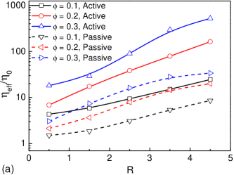
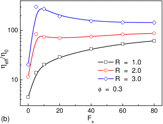
Figure 6: Effective viscosity $\eta_{\text{eff}}$ as a function of (a) particle size $R$ for different values of concentration $\phi=0.1$, 0.2 and 0.3 with fixed active force $F_{a}=20$, and (b) active force $F_{a}$ for different particle size $R=1.0$, 2.0 and 3.0 with fixed concentration $\phi=0.3$. Note that $\eta_{\text{eff}}$ is reduced by the viscosity of pure solution $\eta_{0}$

III.4 Scaling of $D$ with active force $F_{a}$

Another feature shown in Fig.6(b) is that $\eta_{\text{eff}}^{a}$ becomes not sensitive to $F_{a}$ if $F_{a}$ is large enough. Now considering eqn (9) for the long time diffusion constant $D$, one can see that the second term would dominate if $F_{a}$ is large. Therefore, $D$ would scale approximately as $F_{a}^{2}$ in the range of large $F_{a}$. Motivated by this observation, we have also investigated quantitatively how $D$ depends on $F_{a}$ in the whole range.

Surprisingly, we find that $D$ shows a rather good power-law scaling with $F_{a}$, i.e., $D\sim F_{a}^{\alpha}$, as shown in Fig.7(a) for different particle sizes and fixed concentration. For $R=1.0$, 2.0 and 3.0, the scaling exponent $\alpha$ reads approximately 1.40, 1.99 and 2.31, respectively. In Fig.7(b), the dependence of $\alpha$ exponent on particle size $R$ is depicted, where one observes a rather interesting non-monotonic variation: $\alpha$ increases from 1.4 at $R=1.0$ to a maximum value $\alpha\simeq 2.4$ at $R=5.0$ and then decreases again to about 2.2 at $R=7.0$ which is the largest particle size considered in the present work (to get a reliable data at $R>$5.0 that avoiding the finite-size effects, we have to extend the system to $l=30.0\sigma_{0}$ consisting of totally 126 polymers). In the limit of very large particle size, one would imagine that the polymer solution can be viewed as a simple fluid, and the exponent would become 2.0 again.

In the current stage, we are yet not able to understand the power-law scaling between $D$ and the active force $F_{a}$. eqn (9) would simply give $D\sim F_{a}^{2}R/\eta_{\text{eff}}^{a}$ when the active term dominates, which seems to suggest an exponent to be 2.0 if $\eta_{\text{eff}}^{a}$ is not dependent on $F_{a}$. Nevertheless, eqn (9) is just a definition of $\eta_{\text{eff}}^{a}$ which is obtained from the simulated value of $D$, and the calculated values of $\eta_{\text{ef}\text{f}}^{a}$ do depend on $F_{a}$ as already shown in Fig. 6. Therefore, to understand the power-law dependence of $D$ on $F_{a}$, one has to derive a separate theory for the diffusion of ABP in polymer solutions, which is important but beyond the scope of current study.

Here in the present paper, we would like to take a qualitative description to highlight the active effects. According to the MCT framework to study the diffusion of a passive NP in polymer solution, the long time diffusion coefficient can be decomposed into two different parts, i.e., $D=D_{\text{micro}}+D_{\text{hydro}}$, where $D_{\text{hydro}}$ is the conventional SE term, while $D_{\text{micro}}$ is due to the microscopic level interactions between the particle and polymer molecules. The friction related to $D_{\text{micro}}$ results from direct binary collisions between the NP and the polymer beads and density fluctuation of the solution. For large particles in entangled solutions with strong topological constraints, however, one should take into account another possible mechanism for diffusion, namely, the hopping process(Cai et al., 2015), wherein the particle can diffuse by overcoming barrier between neighboring confinement cells. Now we take the particle activity into account. Clearly, enhancement of particle activity would lead to more frequent direct collisions between the particle and polymer beads, thus leading to a larger effective viscosity compare to that experienced by a passive particle. Since we only consider a single particle here, the density fluctuation contribution to the friction would not change much with the variation of the particle activity. Nevertheless, particle activity would facilitate the hopping process if the particle is large enough, which would result in a relatively smaller effective viscosity. Therefore, for a small particle such as $R=1.0$, the effective viscosity experienced by an ABP would increase with the amplitude $F_{a}$, since hopping diffusion is not relevant for small particles. In this case, the scaling exponent $\alpha$ would be less than $2.0$ since $\eta_{\text{eff}}$ scale as $F_{a}^{\lambda}$ with $\lambda>0$. For a large particle such as $R=3.0$, both binary collisions and hopping processes will be enhanced by the particle activity. These two effects competes with each other, leading to the non-monotonic dependence of $\eta_{\text{eff}}^{a}$ with $F_{a}$ as demonstrated in Fig.6(b). In the small $F_{a}$ range, enhanced binary collision dominates leading to an sharp increase of $\eta_{\text{eff}}^{a}$, while for large $F_{a}$, enhanced hopping dominates which results in decrease of $\eta_{\text{eff}}^{a}$. In this case, the exponent $\alpha$ should be larger than 2.0 in the large $F_{a}$ range. For a particle of proper size, the positive and negative effects of particle activity may cancel, which leading to weak dependence of $\eta_{\text{eff}}^{a}$ on $F_{a}$ and the exponent $\alpha$ would be approximately 2.0. For a very large particle size, however, the effect that activity enhances hopping may become weaker than that for a relatively smaller particle, such that $\alpha$ would decrease with $R$. All these features are consistent with the observations in Fig.7(b).

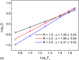
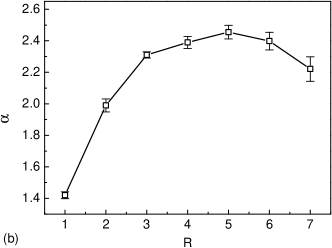
Figure 7: (a)dependence of diffusion coefficient $D$ on propelling force $F_{a}$ in a scaling form. The radius of NP are fixed at $R=1.0,$ 2.0 and 3.0, represented by black, red and blue dots, respectively. The solid lines are scaling fits to the data(b)The scaling factor of the function between $D$ and $F_{a}$ in a fixed size of NP. The solid line is drawn to guide eyes.

IV Conclusion

In conclusion, we have used Langevin Dynamic simulation method to investigate the diffusion behavior of an ABP in semidilute polymer solution. Extensive simulations indicate that the activity can markedly enhance the diffusion of NP in this complex environment, respected to a passive NP. Interestingly, we have found that the dependence of long time diffusion coefficient $D$ on the particle radius $R$ is non-monotonic and $D$ reaches a maximum value at a certain optimal value $R_{opt}$, if exerted a propelling force $F_{a}$ strong enough. Consequently, the NP with a bigger size would get a higher $D$ than a relatively smaller one, which is greatly against the common sense that a larger particle usually diffuse slower for a passive NP.

The subsequent analysis from the short time dynamics reveals that this abnormal phenomenon is due to the two fold impacts of ABP on diffusion. In detail, the increasing size of ABP gains more obstruction from the polymer beads that leads to more apparent cage effects, which finally slows down the diffusion. However, on the other side, a bigger size could usually make the rotation tougher and result in the longer rotational relaxation time $\tau_{p}$. This would lead to longer persistence motion along a direction and cause superdiffusion behavior which would cover the subdiffusion from the cage effect, and finally facilitates the diffusion. It is the competition between the persistence motion and the cage effect that leads to the non-monotonic dependence of the long time diffusion $D$ on the particle size $R$.

We have also introduced a phenomenological model to describe the ABP dynamics, assuming that the ABP is moving in a simple viscous fluid with effective viscosity $\eta_{\text{eff}}^{a}$. We find that this effective viscosity shows strongly dependency on the particle size $R$ as well as active force $F_{a}$. Interestingly, this effective viscosity experienced by the ABP is larger than that experience by a passive nano-particle of the same size, which means that the ABP feels a much more viscoelastic local environment, otherwise it would diffuse much faster. For an ABP of small size, $\eta_{\text{eff}}^{a}$ increases monotonically with $F_{a}$, while for a large ABP, $\eta_{\text{eff}}^{a}$ can even show a non-monotonic dependence on $F_{a}$ bypassing a maximum.

A more striking finding is that $D$ shows a power-scaling with the active force $F_{a}$ in an excellent manner. The exponent $\alpha$ is not equal to the value 2.0 that observed in a simple liquid, but non-monotonically depends on $R$. It increases from a value quite smaller than 2.0 to a maximum value at about 2.5, and then decreases again to 2.0 if $R$ is large enough. Although a rigorous theory for the diffusion behavior of ABP in polymer solutions is not available at the current stage, we have tried to understand the effect of activity on particle diffusion through its influence on the binary collisions between the particle and polymer beads and on the hopping process of a large particle out of confinement cells.

Our results indicate that activity combined with the inner structure of the polymer solution indeed largely affects the diffusion dynamics of an active particle, both short time and long time, which is greatly different to a passive one. We believe that our work can open more perspectives on the study of active matter in complex solutions and may shed some new lights on understanding such an important process in real biological systems.